Identification of Parameters in Photovoltaic Models through a Runge Kutta Optimizer

Abstract

Recently, the resources of renewable energy have been in intensive use due to their environmental and technical merits. The identification of unknown parameters in photovoltaic (PV) models is one of the main issues in simulation and modeling of renewable energy sources. Due to the random behavior of weather, the change in output current from a PV model is nonlinear. In this regard, a new optimization algorithm called Runge–Kutta optimizer (RUN) is applied for estimating the parameters of three PV models. The RUN algorithm is applied for the R.T.C France solar cell, as a case study. Moreover, the root mean square error (RMSE) between the calculated and measured current is used as the objective function for identifying solar cell parameters. The proposed RUN algorithm is superior compared with the Hunger Games Search (HGS) algorithm, the Chameleon Swarm Algorithm (CSA), the Tunicate Swarm Algorithm (TSA), Harris Hawk’s Optimization (HHO), the Sine–Cosine Algorithm (SCA) and the Grey Wolf Optimization (GWO) algorithm. Three solar cell models—single diode, double diode and triple diode solar cell models (SDSCM, DDSCM and TDSCM)—are applied to check the performance of the RUN algorithm to extract the parameters. the best RMSE from the RUN algorithm is 0.00098624, 0.00098717 and 0.000989133 for SDSCM, DDSCM and TDSCM, respectively.

1. Introduction

Researchers are making developments in sources of renewable energy to combat environmental pollution caused by use of fossil fuels. Solar, wind, nuclear and wave energies are the most renewable sources used in our lifetime; hence, researchers all over the world are focused on them [1,2,3,4,5]. Due to the cleanliness and availability of solar energy, it has been recognized as a capable renewable energy source [6]. Generation of electricity directly from solar energy is accomplished by photovoltaic (PV) systems [7] and their behaviour is successfully simulated based on several PV models [8,9]. They have applications such as heating and cooling [10], fuel cells [11], cost-effective emission dispatches [12] and water desalination [13].

There are different electronic circuits that simulate PV systems, such as the single diode solar cell model (SDSCM), the double diode solar cell model (DDSCM) and the triple diode solar cell model (TDSCM). Among them the most commonly used are the SDSCM and the DDSCM [14]. In general the P-N junction is the internal construction of solar cells that has three regions: Defect, space charge and quasi-neutral regions. The diffusion and recombination of the charge transporter causes losses in these regions. The losses in SDSCM can be identified by the losses of the quasi-neutral region. The losses in DDSCM can be identified by the losses of the quasi-neutral and space charge regions. The losses in TDSCM can be identified by the losses of the quasi-neutral, space charge and defect regions [15,16].

The estimation of parameters in PV modules is one of the important items in the development of solar energy. This occurs due to the nonlinear behaviour of the relationship between current and voltage; such variables as outputs are crucial in solar cells [17,18]. The number of the computed parameters varies according to the model used; for SDSCM, DDSCM and TDSCM the number of variables is five, seven and nine, respectively. They are extracted with two passes: The first way is the traditional analytic method and the second way is with the use of meta-heuristics algorithms. The traditional analytic methods are considered a typical solution in estimating the solar cell variables, such as Lambert W-functions [19], Gauss Seidel technique [20,21], the Newton–Raphson method [22], the least square method [23] and the conductivity method (CM) [24].

With the development of computer and artificial intelligence, several meta-heuristics methods have been applied in extensive fields, especially in complex and nonlinear optimization problems [25,26]. Due to the nonlinearity of the behaviour of photovoltaic problems, metaheuristics techniques have been applied widespread in the problem of parameter estimation of PV cells. Meta-heuristics techniques are introduced and classified into four branches, i.e., sociology-based methods, physics-based methods, biology-based methods and mathematics-based methods [27]. The algorithms of sociology used in the identification of PV parameters are the Harmony search algorithm [28], Teaching learning-based optimization and its improvement [29,30], the Imperialist competitive algorithm [31] and the multiple learning backtracking search algorithm [32]. The physics-based methods used in the estimation of PV parameters are the Chaos optimization algorithm with its improvements [33,34], the Simulated annealing algorithm [35], the Fireworks algorithm [36], the Wind driven optimization algorithm [37], the Evaporation rate-based water cycle algorithm [38] and the Lozi map-based chaotic optimization algorithm [39]. The techniques that are biology based and employed for the estimation PV parameters are Particle swarm optimization and its variants [40,41,42,43], the Genetic algorithm [44], Differential evolution [45], Artificial bee swarm optimization [46], Artificial bee colony (ABC) optimization [47], the Whale optimization algorithm [48], the Improved ant lion optimizer [49], Biogeography-based optimization [50], the Cuckoo search (CS) algorithm [51], the Bird mating optimization (BMO) algorithm [52], the Flower pollination algorithm [53], the Grey wolf optimizer (GWO) algorithm [54], the Bacterial foraging algorithm [55] and the Slap swarm algorithm [56]. Other interesting meta-heuristics approaches for the extraction of PV parameters are Pattern search [57], the Shuffled complex evolution (SCE) algorithm [58], the Turbulent flow of water algorithm [59,60] and the JAYA algorithm [61,62].

This article introduces the use of a meta-heuristic algorithm called Runge–Kutta optimizer (RUN), which is applied to extract the solar cell parameter. Here the objective function of the estimation problem is the root mean square error between the experimental recorded current data and the simulated current data based on the parameters extracted from the algorithms. The solar cell models used in this article are the SDSCM, DDSCM and SDSCM. The experiments conducted include comparisons between the RUN algorithm and another six algorithms: the Hunger Games Search (HGS) algorithm [63], the Tunicate Swarm Algorithm (TSA) [64], Harris Hawks Optimization (HHO) [65], the Sine–Cosine Algorithm (SCA) [66], the Chameleon Swarm Algorithm (CSA) [67] the and Grey Wolf Optimizer (GWO) [68]; the dataset from the R.T.C France cell is used. The experiments also include a statistical analysis to measure the performance evaluation of the proposed RUN algorithm and all competitor algorithms. This analysis contains several points such as the minimum, maximum, mean and standard deviation of the objective function over 30 independent runs. Finally a Friedman rank test is performed for the proposed RUN algorithm and all competitor algorithms in all cases study. The experiments conducted then validate the performance of the proposed approach based on the RUN algorithm to search for the optimal configuration of the parameters.

The goals of this article are listed as follows:

• Introduce an alternative method to identify the parameters in solar cells using the RUN algorithm in combination with the diode models.
• Test the RUN algorithm over a real multidimensional problem.
• Accurately identify the best parameters in solar cells by using a modern metaheuristic.

This paper is organized as follows: The mathematical formulation of three photovoltaic diode models is described in Section 2. Section 3 discusses the objective function for the estimation of the photovoltaic parameters. Section 4 presents the Runge–Kutta optimizer (RUN). The experimental results are discussed in Section 5. The conclusions of the article are presented in Section 6.

2. Mathematical Photovoltaic Models for Solar Cells

This section analyses the mathematical formulation for the three models of photovoltaics: the Single diode solar cell model (SDSCM), the double diode solar cell model (DDSCM) and the triple diode solar cell model (TDSCM).

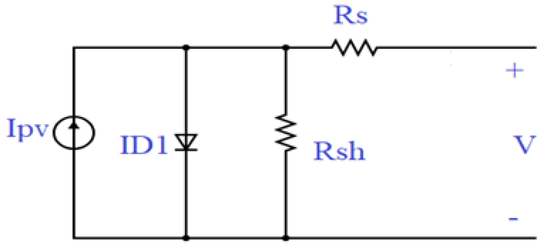
2.1. Single Diode Solar Cell Model

Figure 1 shows the equivalent circuit of the single diode solar cell model. Based on this diagram the mathematical equation for SDSCM is defined as follows:

$$I=I_{pv}-I_{D1}-I_{sh}$$

(1)

$$I=I_{pv}-I_{h1}[e^{\frac{q(V+I{R}_s)}{n_{1}K{T}_c}}]-\frac{V+I{R}_s}{R_{sh}}$$

(2)

The output current of SDSCM is I, $I_{pv}$ is the generated photo-current, the current in shunt resistor is $I_{sh}$, $I_{D1}$ is the current in the first diode, $R_{sh}$ is the resistance shunted with the diode terminal, $R_s$ is the series resistance, $n_1$ is the diode ideality factor, the Boltzmann constant is K, the charge of electron is defined by q, $I_h$ is the diode reverse saturation current and the cell temperature is $T_c$.

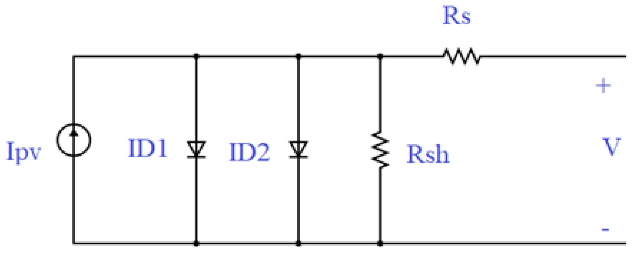
2.2. Double Diode Solar Cell Model

Figure 2 presents the equivalent circuit of DDSCM. Considering the circuit the DDSCM can be defined in the following equation:

$$I=I_{pv}-I_{D1}-I_{D2}-I_{sh}$$

(3)

$$I=I_{pv}-I_{h1}[e^{\frac{q(V+I{R}_s)}{n_{1}K{T}_c}}-1]-I_{h2}[e^{\frac{q(V+I{R}_s)}{n_{2}K{T}_c}}-1]-\frac{V+I{R}_s}{R_{sh}}$$

(4)

where $I_{D2}$ is the second diode current and $n_2$ is the second diode ideality factor.

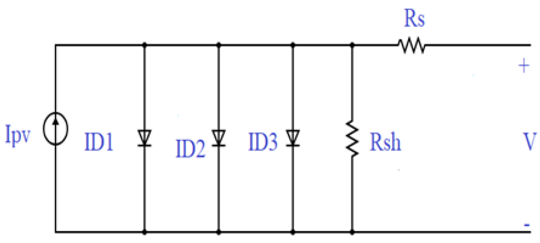
2.3. Triple Diode Solar Cell Model

In Figure 3 is presented the circuit that defines the TDSCM. In Equation (5) the TDSCM is mathematically defined

$$I=I_{pv}-I_{D1}-I_{D2}-I_{D3}-I_{sh}$$

(5)

$$I=I_{pv}-I_{h1}[e^{\frac{q(V+I{R}_s)}{n_{1}K{T}_c}}-1]-I_{h2}[e^{\frac{q(V+I{R}_s)}{n_{2}K{T}_c}}-1]-I_{h3}[e^{\frac{q(V+I{R}_s)}{n_{3}K{T}_c}}-1]-\frac{V+I{R}_s}{R_{sh}}$$

(6)

where the current passes in the third diode are $I_{D3}$ and $n_3$ is the third diode ideality factor.

3. Problem Definition

The two effective matters in any optimization problem are the objective function and boundary limits of the search space. In this paper, the objective function of this problem concerns the minimization of the root mean square error (RMSE) between the experimental recorded current data and the current data extracted from the simulation. The mathematical definition of the RMSE is presented in the following equation:

$$J(V,I,X)=I_{sim}-I_{exp}$$

(7)

$$\mathrm{RMSE}=\sqrt{\frac{1}{N}\sum _{i=1}^N{\left(J(V,I,X)\right)}^2}$$

(8)

where $I_{exp}$, the experimental recorded current data, N is the number of reading data, X is variable with the extracted parameters and $I_{sim}$ corresponds to the estimated current obtained by one of the diode models. For the SDSCM the variables to be identified are X = ($R_s$, $I_{h1}$, $n_1$, $R_{sh}$ and $I_{pv}$). In the DDSCM the variables to be extracted are X = ($R_s$, $I_{h1}$, $n_1$, $R_{sh}$, $I_{pv}$, $I_{h2}$ and $n_2$). Finally, for the TDSCM the elements to be identified are X = ($R_s$, $I_{h1}$, $n_1$, $R_{sh}$, $I_{pv}$, $I_{h2}$, $n_2$, $I_{h3}$ and $n_3$). The lower and upper boundaries of the variables for all the models are reported in

Table 1. The variables’ lower and upper boundaries.

Parameters	Lower Bound	Upper Bound
$I_{pv}$	0	1
$I_{h1}$, $I_{h2}$ and $I_{h3}$ $\left(\mathsf{\mu }\mathrm{A}\right)$	0	1
$R_s$	0	0.5
$R_{sh}$	0	100
$n_1$, $n_2$ and $n_3$	1	2

.

4. The Runge–Kutta Optimizer

This section introduces a brief description of the Runge–Kutta optimizer (RUN) optimization algorithm [69]. The RUN is based on the theory of the Runge–Kutta method that is employed for solving ordinary differential equations in numerical methods. The RUN has two stages; the first is the search procedure that uses the Runge–Kutta theory and the second is called enhanced solution quality (ESQ). The following subsection will explain the basics of the RUN.

4.1. Updating Solutions

The RUN algorithm uses a search mechanism (SM), see Appendix A, based on the Runge–Kutta method to update the position of the current solution at each iteration, which is defined Algorithm 1.

Algorithm 1 Search mechanism (SM) to update the position of current solution used in RUN

if$rand<$ 0.5 then            (exploration phase)            $X_{n+1}=(X_c+r\times SF\times g\times x_c)+SF\times SM+\mu \times (randn\times (x_m-x_c))$      else            (exploration phase)            $X_{n+1}=(X_m+r\times SF\times g\times x_m)+SF\times SM+\mu \times (randn\times (x_{r1}-x_{r2}))$      end if

From the previous explanation r is an integer number that takes the values of 1 or −1 and helps to improve the diversity. g is a random number in the range [0, 2]; also $\mu$ is a random number too. The formula to compute SM is defined in Appendix A. Finally $SF$ is an adaptive factor that is computed as follows:

$$SF=2.(0.5-rand)\times f$$

(9)

$$F=a\times exp(-b\times rand\times \left(\frac{i}{Maxi}\right))$$

(10)

where $Maxi$ stands for the largest number of iterations. Besides, the values of $x_c$ and $x_m$ are as follows:

$$x_c=\varphi \times x_n+(1-\varphi )\times x_{r1}$$

(11)

$$x_m=\varphi \times x_{best}+(1-\varphi )\times x_{lbest}$$

(12)

From Equations (11) and (12), $\varphi$ is a random number in the range of (0,1). $x_{best}$ is the best-so-far solution. $x_{lbest}$ is the best position obtained at each iteration.

4.2. Enhanced Solution Quality

In the RUN algorithm, the enhanced solution quality (ESQ) is a step employed to increase the quality of the solutions and avoid local optima in each iteration. The scheme shown in Algorithm 2 is executed to create the solution ($x_{new2}$) by using the ESQ:

Algorithm 2 Scheme to create the solution ($x_{new2}$) by using the ESQ in RUN

if$rand<$ 0.5 then            if $w<1$ then                    $x_{new2}=x_{new1}+r.w.\left|(x_{new1}-x_{avg})+randn\right|$                else                    $x_{new2}=(x_{new1}-x_{avg})+r.w.\left|(u.x_{new1}-x_{avg})+randn\right|$                end if      end if

From the previous steps, the values of w, $x_{avg}$ and $x_{new}$ are computed by using the following equations:

$$w=rand(0,2).exp(-c\left(\frac{i}{Maxi}\right))$$

(13)

$$x_{avg}=\frac{x_{r1}+x_{r2}+x_{r3}}{3}$$

(14)

$$x_{new1}=\beta \times x_{avg}+(1-\beta )\times x_{best}$$

(15)

where $\beta$ is a random number defined in the range [0, 1]. $c=5\times rand$, where $rand$ is a random value. r is an integer number that could take the values 1, 0 or −1. $x_{best}$ is the best solution explored so far. The solution $x_{new2}$ does not always have a better fitness than the current solutions. In this case, the RUN provides another opportunity to enhance the fitness by using $x_{new3}$. This procedure is performed as shown in as Algorithm 3.

Algorithm 3 Enhancing the new solution $x_{new3}$

if$rand<w$then            $x_{new3}=(x_{new2}-rand{x}_{new2})+SF.(rand.x_{RK}+(v.x_b-x_{new2}))$      end if

where v is a random number with a value of $2rand$.The pseudo-code of the standard RUN is presented in Algorithm 4.

Algorithm 4 The pseudo-code of RUN

Stage 1. Initialization Initialize a, b Generate the RUN population $X_n$ (n = 1,2,…,N) Calculate the objective function of each member of population Determine the solutions $x_w,x_b,$ and $x_{best}$ Stage 2. RUN operators for$i=1:Maxi$do          for $n=1:N$ do                  for $l=1:D$ do                          Updating solutions                          Calculate position $x_{n+1,l}$ according to Section 4.1                       end for                    Enhance the solution quality                    if rand < 0.5 then                          Calculate position $x_{new2}$ as in Section 4.2                          if f($x_n$)<f($x_{new2}$) then                                  if rand < w then                                          Calculate position $x_{new3}$ using the explanation provided in Section 4.2                                      end if                              end if                       end if                    Update positions $x_w$ and $x_b$                end for            Update positions $x_{best}$            $i=i+1$      end for Stage 3. return $x_{best}$

5. Experimental Results

This section explains the identified parameters for the SDSCM, DDSCM and TDSCM models using the RUN algorithm. The proposed implementation for the RUN algorithm is compared with other meta-heuristic approaches such as the Hunger Games Search (HGS) algorithm [63], the Tunicate Swarm Algorithm (TSA) [64], Harris Hawks Optimization (HHO) [65], the Sine–Cosine Algorithm (SCA) [66], the Chameleon Swarm Algorithm (CSA) [67] and the Grey Wolf Optimizer (GWO) algorithm [68]. The recorded R.T.C France solar cell data at 1000 w/m² solar radiation and 33 °C temperature is applied to evaluate the algorithms’ accuracy and reliability and accuracy.

Each algorithm’s settings are described in

Table 2. Parameter setting for all the algorithms used in the comparative study.

Algorithms	Parameter Setting
General Setting	Population size: $N=30$
	Maximum iterations: $t_{max}=1000$
RUN	a = 20 and b = 12
HGS	l = 0.08 and hunger threshold (LH) as 10, 100, 1000 and 1000
TSA	$P_{min}$ = 1 and $P_{max}$ = 4
HHO	$beta=$ 1.5
SCA	A = 2
CSA	$p1,p2,0.25,1.50,1.0,c1,c21.75,1.75$
GWO	Control Parameter $\left(a\right)$ is [2, 0]

for clear comparison.

The next subsections will present and discuss the experimental results obtained by the SDSCM, the DDSCM and the TDSCM. A statistical analysis is also conducted; the outcomes are also discussed in a respective subsection.

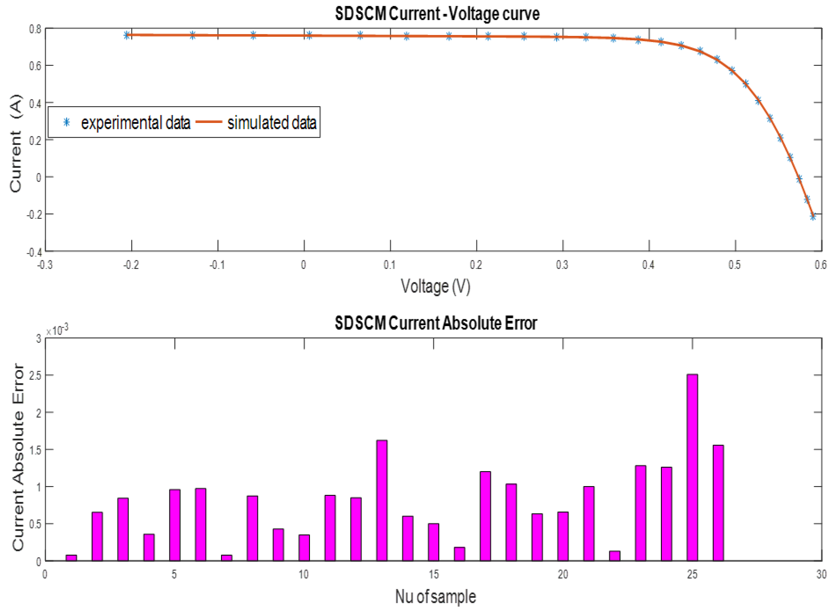
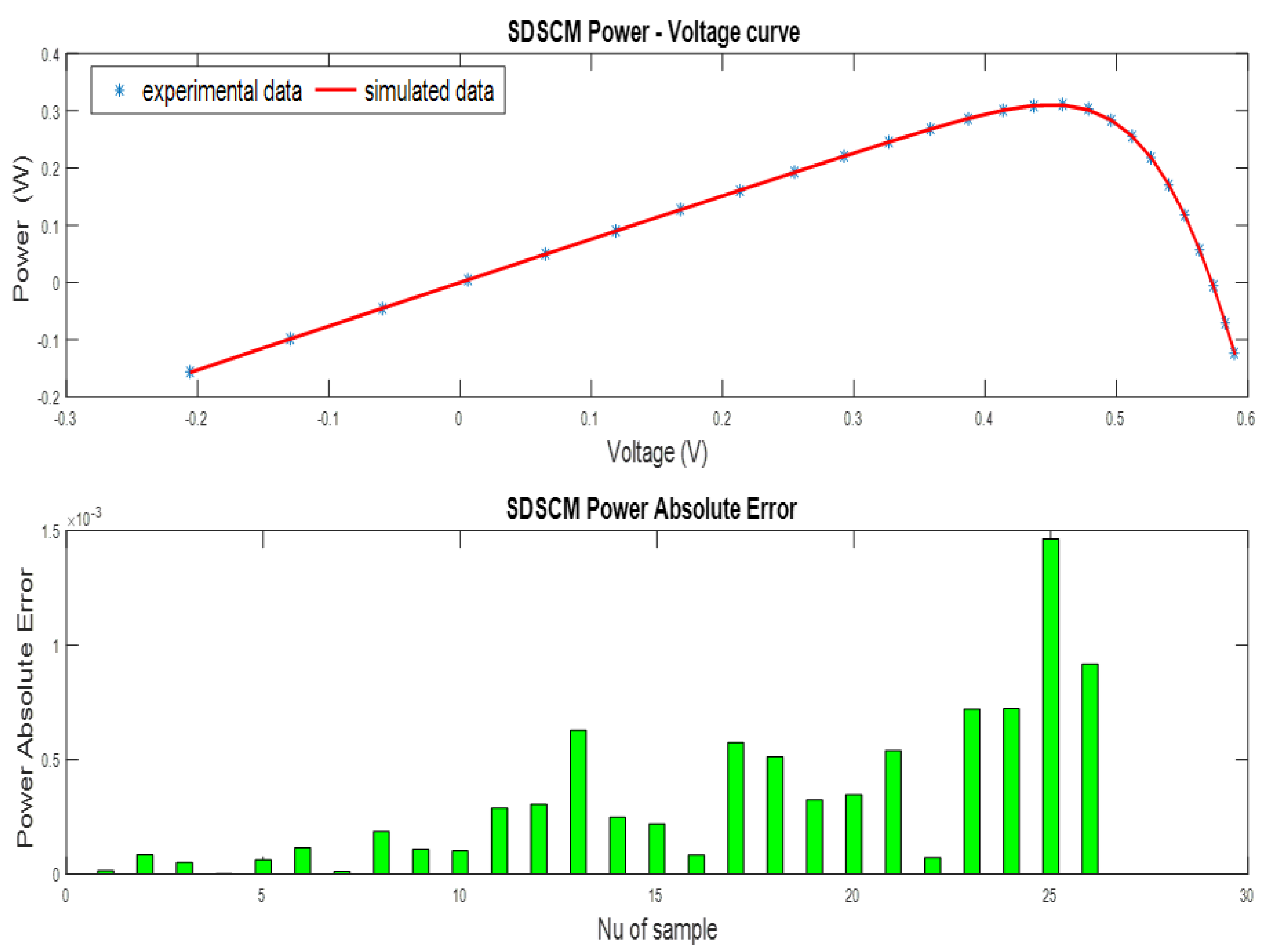
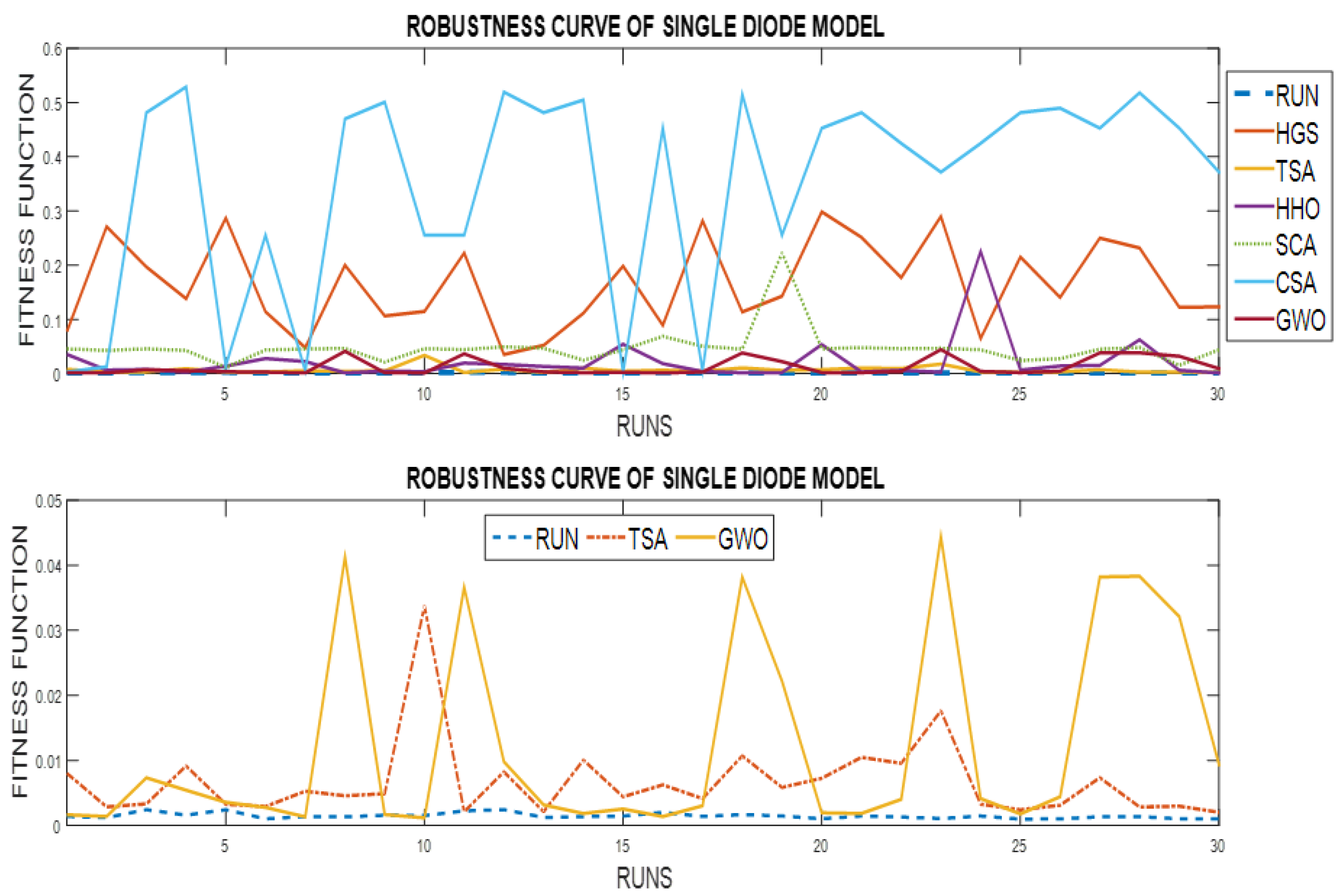
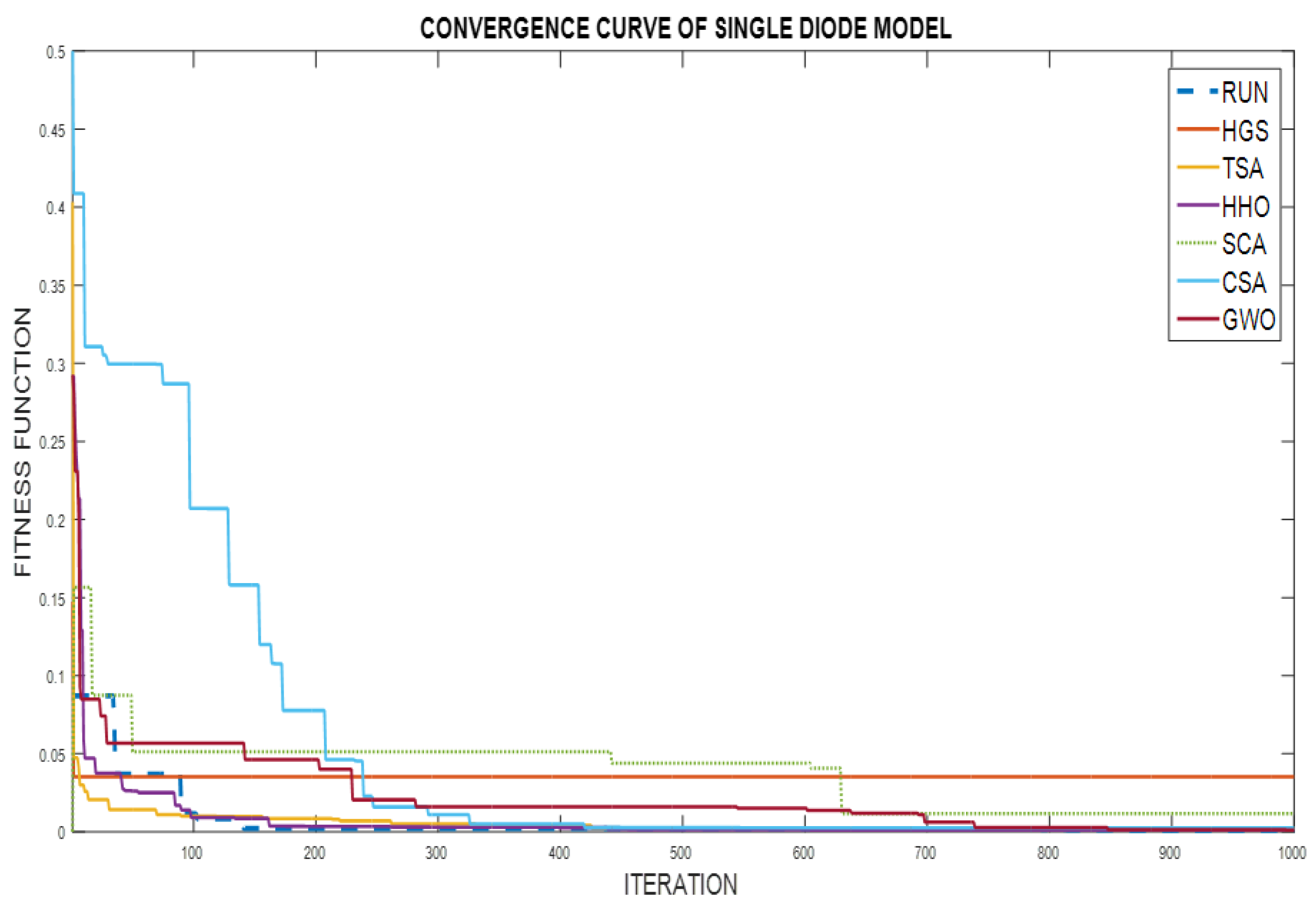
5.1. Results of SDSCM

The results of the decision parameters for SDSCM estimated by implementing the RUN algorithm and the comparison with the other method for finding the best RMSE are illustrated in

Table 3. The parameters estimated for SDSCM at the optimum RMSE.

Algorithm	${\mathit{I}}_{\mathit{p}\mathit{v}}$ (A)	${\mathit{I}}_{\mathit{h}1}$ (A)	${\mathit{n}}_1$	${\mathit{R}}_{\mathit{s}}$ ($\Omega )$	${\mathit{R}}_{\mathit{s}\mathit{h}}$ ($\Omega$)	RMSE
RUN	0.76076384	3.20 × 10${}^{-7}$	1.4802504	0.03641606	53.6707057	0.00098624
HGS	0.74385157	1.00 × 10${}^{-6}$	1.59848349	0.02112377	100	0.03531608
TSA	0.76156952	3.18 × 10${}^{-7}$	1.47990458	0.0370102	56.8748349	0.00203122
HHO	0.76061081	4.69 × 10${}^{-7}$	1.51967855	0.03494388	67.4858973	0.00122548
SCA	0.7604604	8.14 × 10${}^{-7}$	1.58164936	0.02603417	85.9162977	0.0115909
CSA	0.76297186	6.70 × 10${}^{-7}$	1.55923486	0.0326915	41.6278317	0.00257795
GWO	0.76136271	3.59 × 10${}^{-7}$	1.49183006	0.03607813	49.6793825	0.00117546

. The optimization method that achieves the best RMSE of value 0.000986242 is the RUN algorithm, this value is in a bold number in Table 3. The order of algorithms based on the minimum value of the RMSE is RUN, GWO, HHO, TSA, CSA, SCA and HGS. The I-V and P-V characteristics of the tested SDSCM are performed based on the extracted results from the RUN algorithm in Table 3. Figure 4 shows the I-V curve and the absolute error of current (AEI) for SDSCM based on the extracted data from the RUN algorithm. Figure 5 introduces the P-V curve and the absolute error of power (AEP) for SDSCM based on the extracted data from the RUN algorithm. Based on Figure 4 and Figure 5 the minimum value of the absolute current error is 0.0000764260676708872 and the minimum value of absolute power error is 0.0000020451684640101. The error values presented before can be interpreted with a high degree of accuracy due to the optimal configuration of parameters obtained by using the RUN algorithm. Moreover, Figure 4 and Figure 5 explain the high closeness between the simulated and experimental recorded data so that the proposed RUN algorithm achieves high performance and more accuracy in extracting the decision variables of SDSCM. Both Figure 4 and Figure 5 use the number of samples (Nu of samples) to show the absolute error computed for each variable. Besides, for Figure 4 and Figure 5 the data is also taken from the manufacturer of the R.T.C France solar cell; this information is used for the three diode models.

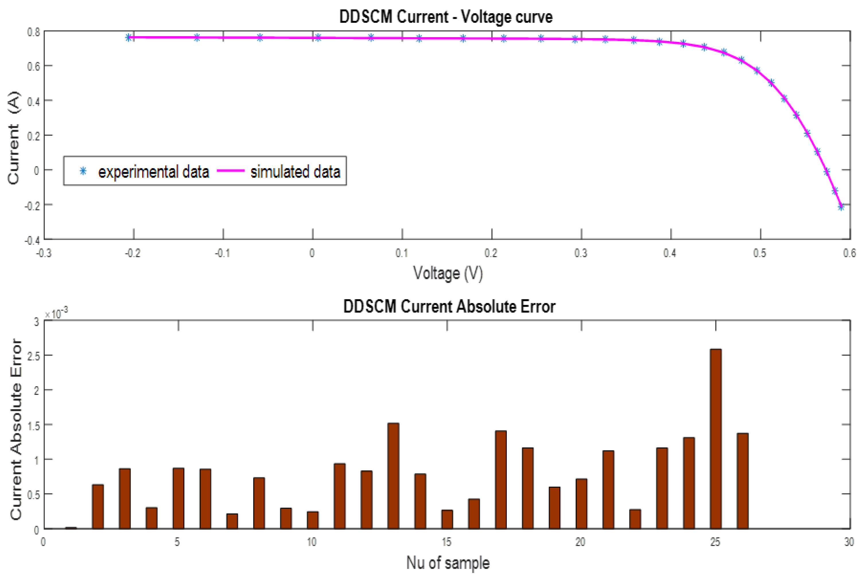
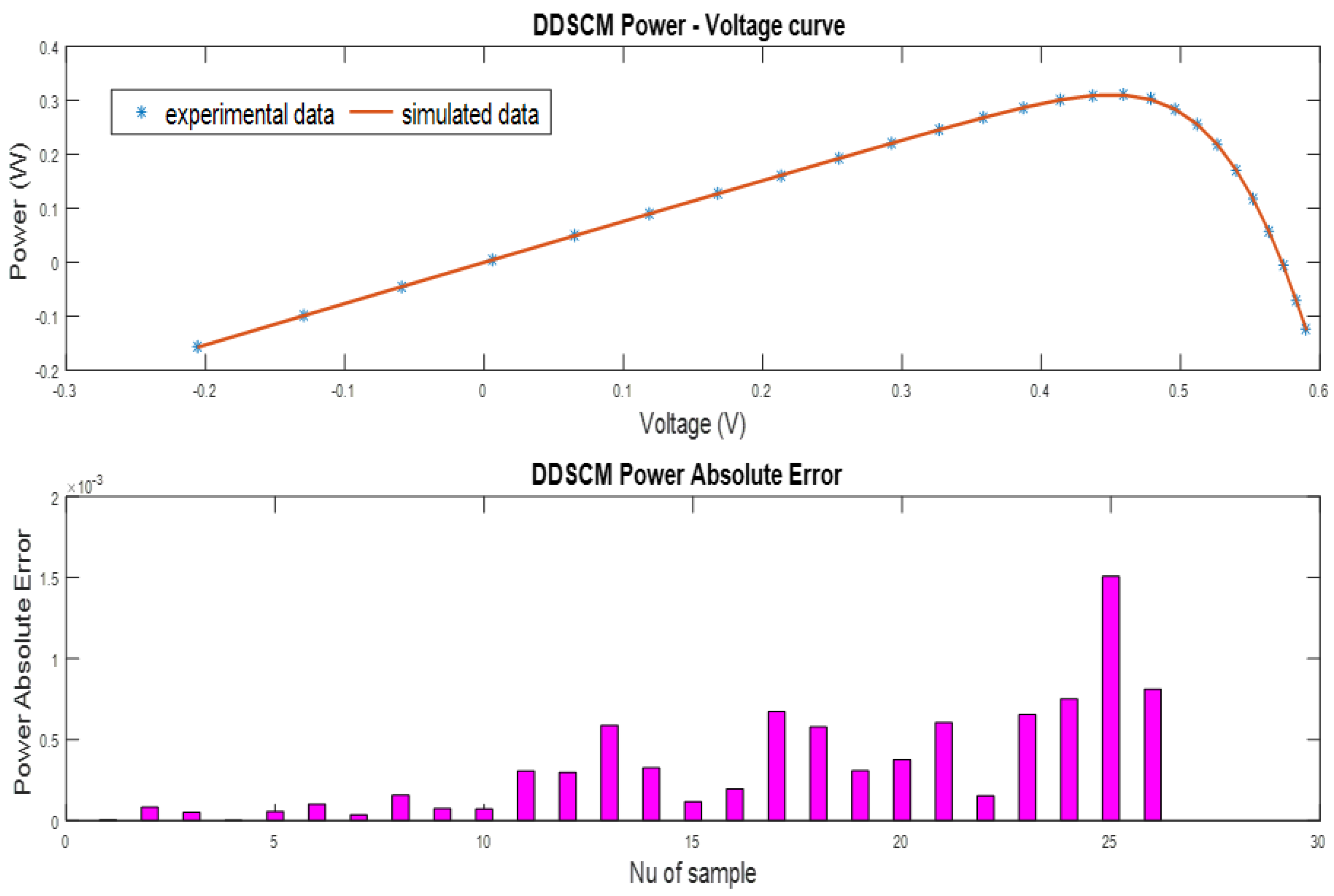
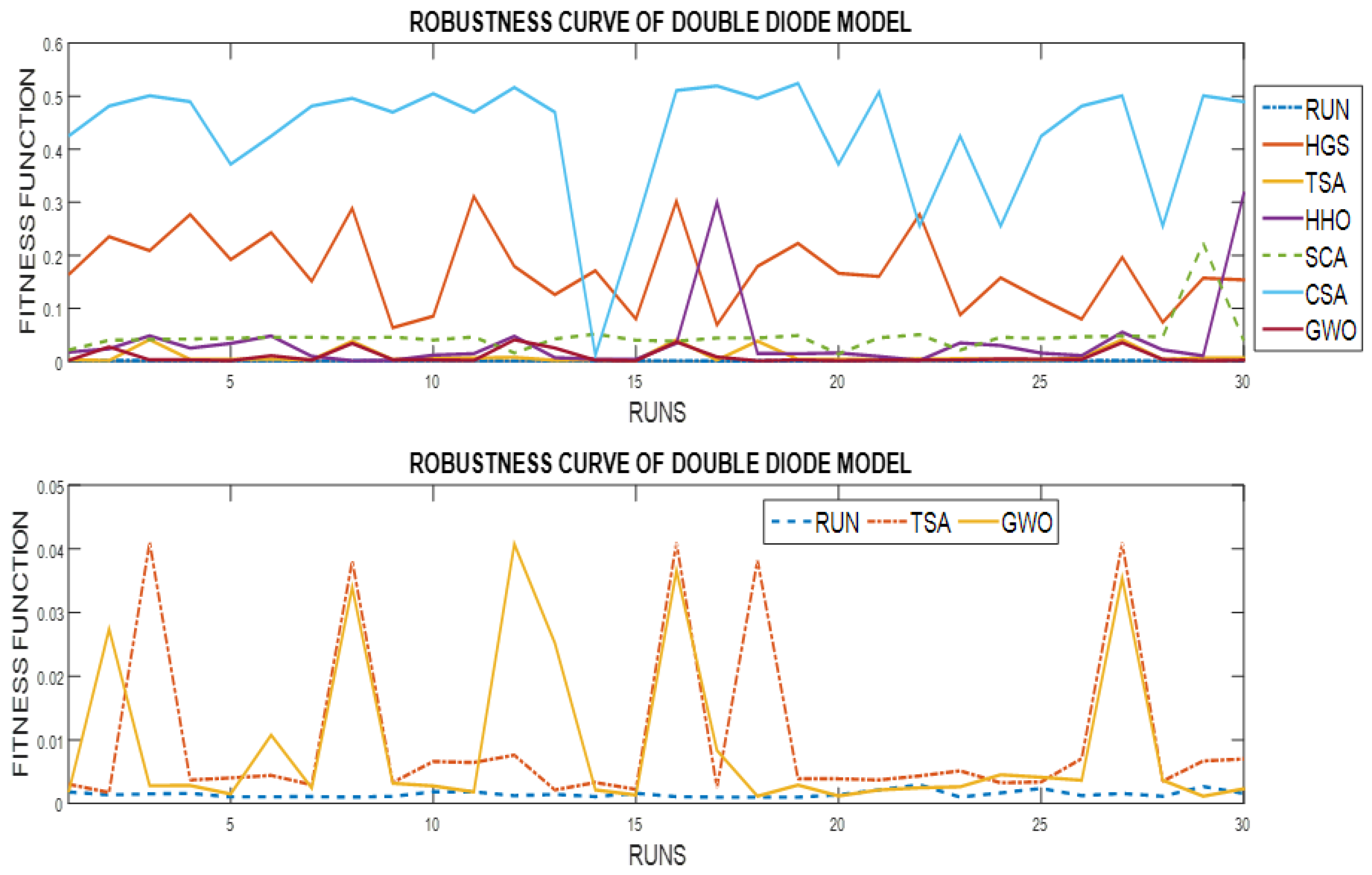
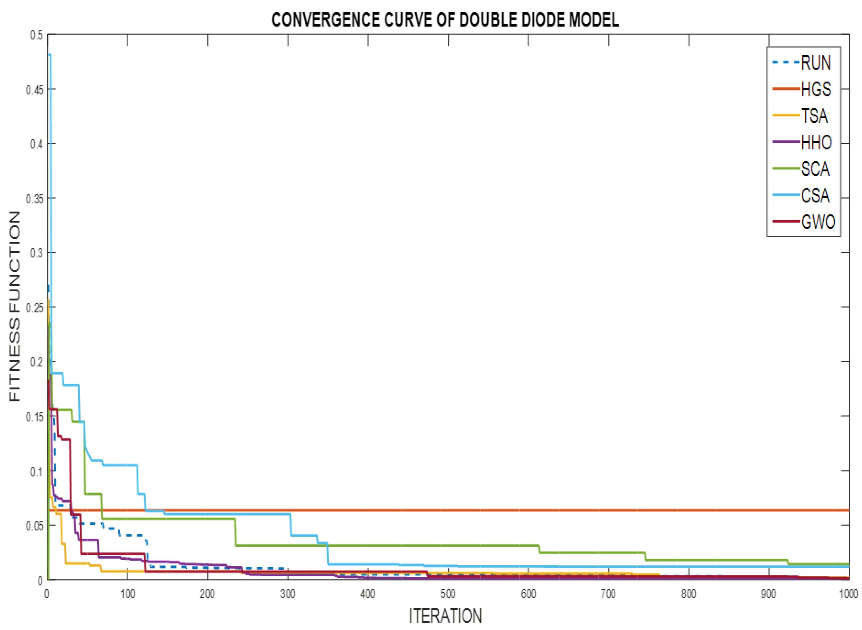
5.2. Results of DDSCM

The results of the variables of DDSCM estimated using the RUN optimizer and its comparison with the rest of the algorithms to obtain the optimal RMSE are illustrated in

Table 4. The parameters estimated for DDSCM at the optimum RMSE.

Algorithm	${\mathit{I}}_{\mathit{p}\mathit{v}}$ (A)	${\mathit{I}}_{\mathit{h}1}$ (A)	${\mathit{n}}_1$	${\mathit{R}}_{\mathit{s}}$ ($\Omega )$	${\mathit{R}}_{\mathit{s}\mathit{h}}$ ($\Omega$)	${\mathit{I}}_{\mathit{h}2}$ (A)	${\mathit{n}}_2$	RMSE
RUN	0.76080253	2.60 × 10${}^{-7}$	1.46347838	0.03644583	55.3832189	5.58 × 10${}^{-7}$	1.9996951	0.00098717
HGS	0.81823842	8.20 × 10${}^{-7}$	1.91014321	0.01747588	96.1240825	8.96 × 10${}^{-7}$	1.60014594	0.06355214
TSA	0.76107259	1.97 × 10${}^{-7}$	1.43559704	0.03812573	45.9993712	1.02 × 10${}^{-7}$	1.78946036	0.00173618
HHO	0.76067423	7.20 × 10${}^{-7}$	1.97316883	0.03603221	55.2632427	2.39 × 10${}^{-7}$	1.45717416	0.00120124
SCA	0.77891309	0.00 × 10${}^0$	1	0.03447825	77.6623318	7.55 × 10${}^{-7}$	1.56931291	0.01419336
CSA	0.78200704	2.22 × 10${}^{-7}$	1.48090338	0.04035768	11.9328948	8.13 × 10${}^{-11}$	1.00028149	0.01193056
GWO	0.761576619	7.71 × 10${}^{-8}$	1.403358962	0.03649657	47.83932117	3.18 × 10${}^{-7}$	1.561920572	0.001149198

. The algorithm that obtains the optimal RMSE is the RUN and the value achieved is 0.000987168, this value is in a bold number in Table 4. The compared approaches can be ranked according to the minimum value of RMSE obtained. The rank for the DDSCM from the lower to the upper value is RUN, GWO, HHO, TSA, CSA, SCA and HGS. The I-V and P-V characteristics of the tested DDSCM are performed based on the extracted results from the RUN algorithm in Table 4. In Figure 6 are plotted the I-V curve and the absolute error of current (AEI) for DDSCM based on the extracted data from the RUN algorithm. Figure 6 explains the P-V curve and the absolute error of power (AEP) for DDSCM based on the extracted data from the RUN algorithm. Based on Figure 6 and Figure 7 the lower value of absolute current error is 0.0000146823091732307 and the lower value of absolute power error is 0.00000171970722786467. The error values presented before can be interpreted with a high degree of accuracy due to the optimal configuration of parameters obtained by using the RUN algorithm. Moreover, these figures explain the high closeness between the simulated and experimental recorded data so that the proposed RUN algorithm achieves high performance and more accuracy in extracting decision variables of DDSCM. Notice that for Figure 6 and Figure 7 Nu of samples refers to the number of samples used to compute the absolute error of the variables.

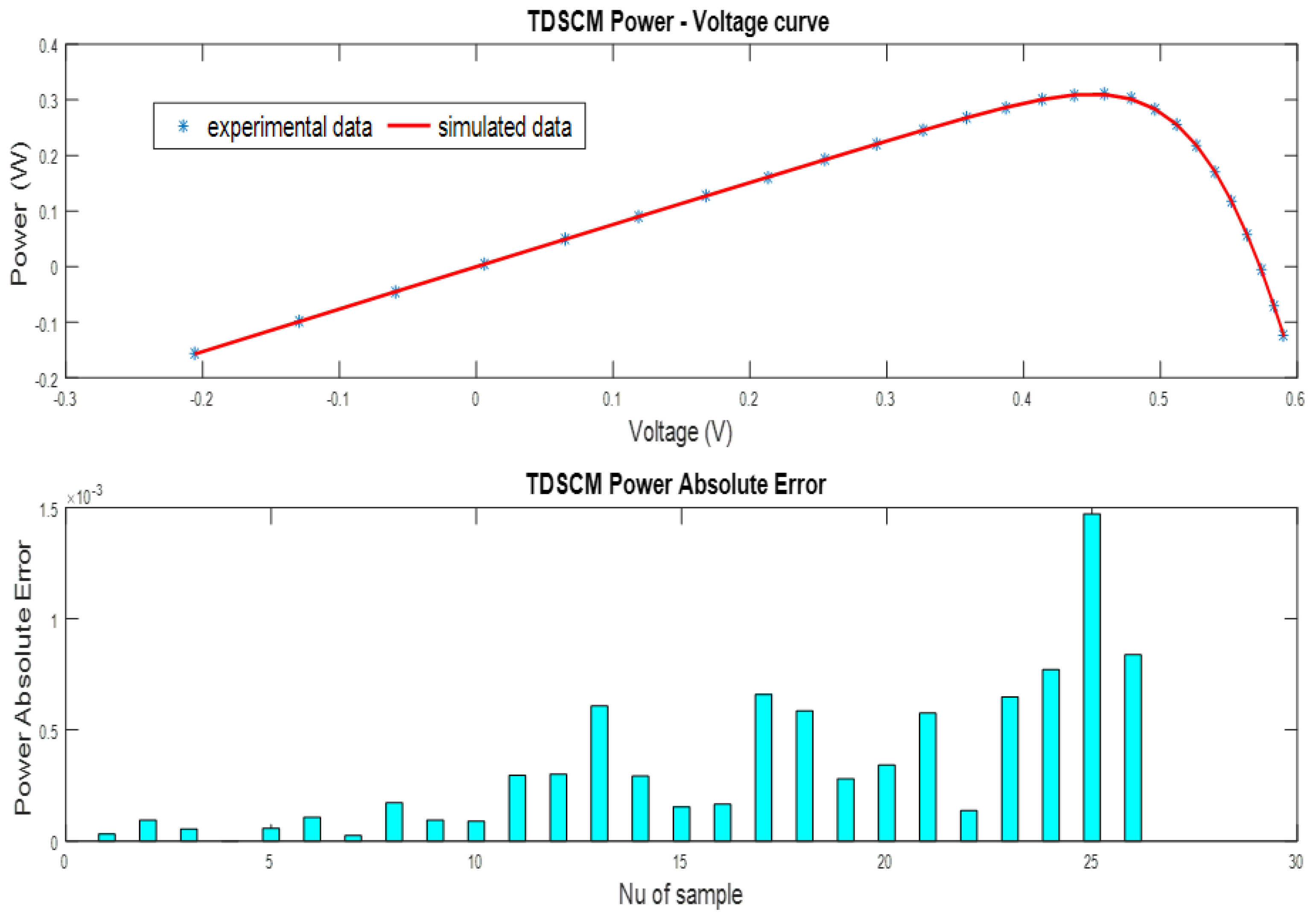
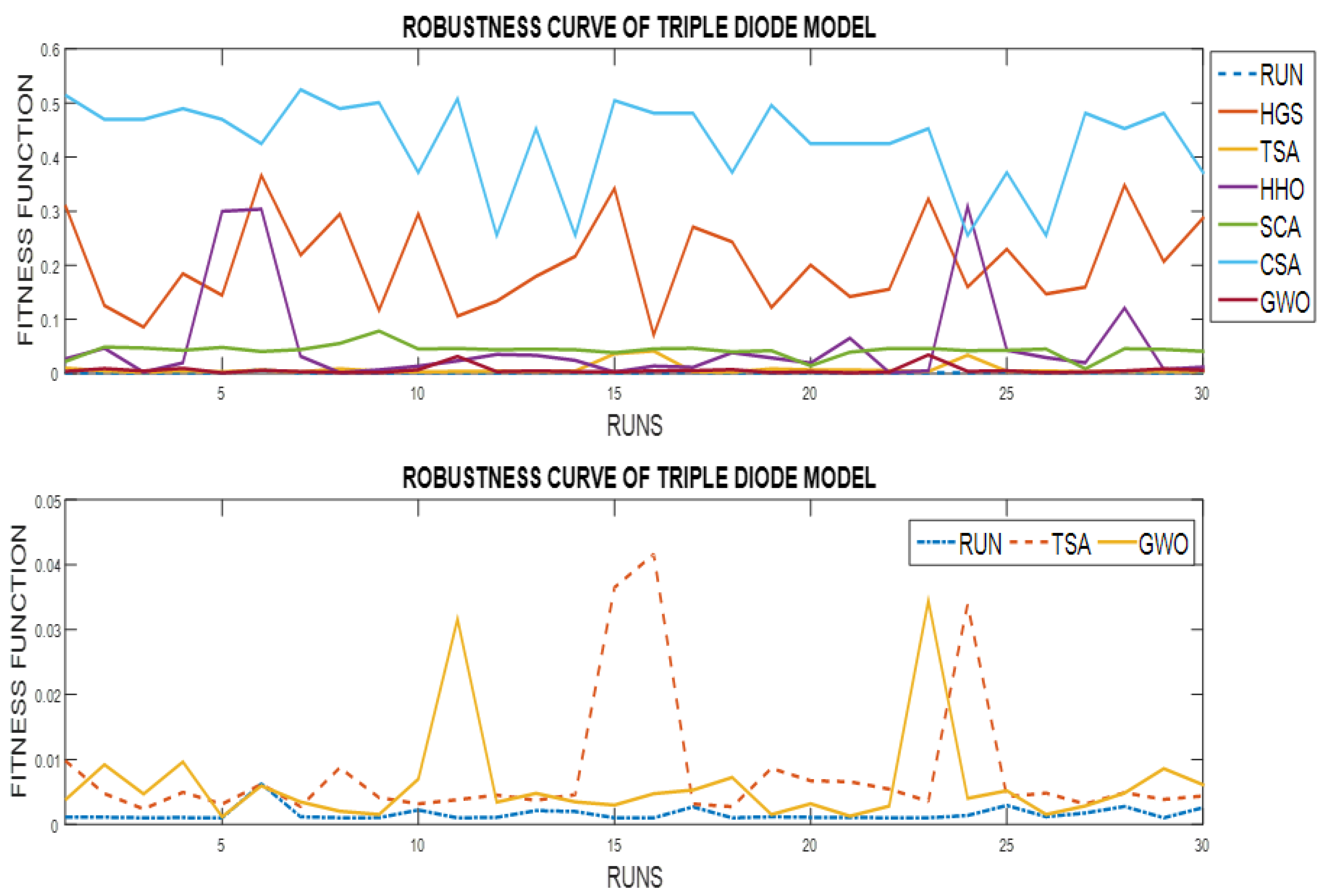
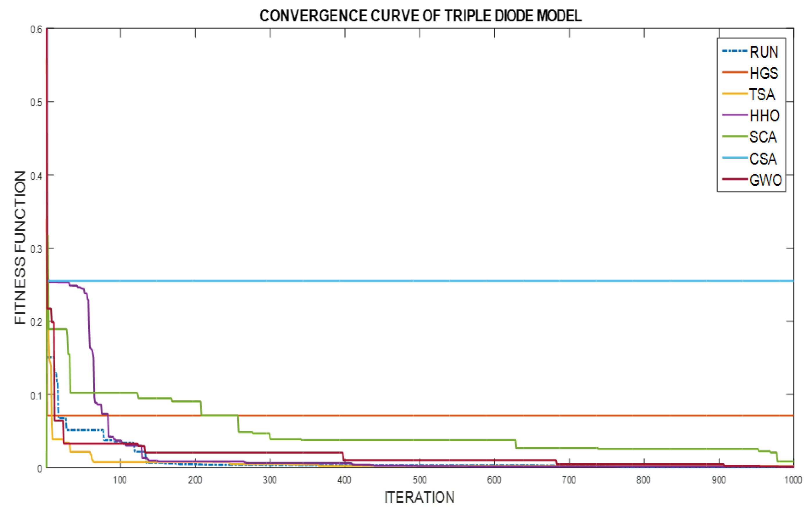
5.3. Results of TDSCM

For the TDSCM the values estimated by all the optimizers in a comparative way including the RMSE are presented in

Table 5. The parameters estimated for TDSCM at the optimum RMSE.

Algorithm	RUN	HGS	TSA	HHO	SCA	CSA	GWO
$I_{pv}$ (A)	0.760836723	0.676357	0.76062	0.760586261	0.752424353	1	0.760301041
$I_{o1}$ (A)	3.30 × 10${}^{-12}$	0.00 × 10${}^{-0}$	3.36 × 10${}^{-7}$	4.73 × 10${}^{-7}$	0.00 × 10${}^{-0}$	0	1.13 × 10${}^{-7}$
$h_1$	1.071707468	1.41 × 10${}^{-0}$	1.95 × 10${}^{-0}$	1.548414761	1.018265918	2	1.448610196
$R_{se}$ ($\Omega$)	0.036313464	0	0.035140703	0.033963588	0.033849004	0	0.036999781
$R_{pa}$ ($\Omega$)	53.61258389	42.80501301	70.67294667	80.40353241	44.21581797	1	51.96432007
$I_{o2}$ (A)	2.65 × 10${}^{-7}$	5.00 × 10${}^{-7}$	9.69 × 10${}^{-7}$	5.96 × 10${}^{-8}$	0.00 × 10${}^{-0}$	0	2.85 × 10${}^{-7}$
$h_2$	1.473397186	2	2	1.513719557	1	1	1.864822779
$I_{o3}$ (A)	8.42 × 10${}^{-8}$	3.67 × 10${}^{-7}$	2.59 × 10${}^{-7}$	8.70 × 10${}^{-8}$	5.30 × 10${}^{-7}$	0	1.02 × 10${}^{-7}$
$h_3$	1.572964526	1.520098844	1.468342094	1.59632106	1.535332708	1	1.442016383
RMSE	0.000989133	0.071278042	0.002362367	0.001625332	0.008624898	0.255247472	0.00115177

. The best RMSE value is 0.000989133 and it is reached by the RUN algorithm, this value is in a bold number in Table 5. The rank of the optimization methods based on its performance using the RMSE as objective function is RUN, GWO, HHO, TSA, SCA, HGS and CSA, where they are sorted from the minimum to the maximum value. The I-V and P-V characteristics of the tested TDSCM are computed by using the parameters obtained by the RUN method and they are shown in Table 5. Figure 8 explains the I-V curve and the absolute error of current (AEI) for TDSCM based on the extracted data from the RUN algorithm. Figure 9 explains the P-V curve and the absolute error of power (AEP) for TDSCM based on the extracted data from the RUN algorithm. Based on Figure 8 and Figure 9 the minimum value of the absolute current error is 0.000144871336086205 and the minimum value of the absolute power error is 0.00000162546142774399. The error values presented before can be interpreted with a high degree of accuracy due to the optimal configuration of parameters obtained by using the RUN algorithm. Moreover, these figures explain the high closeness between the simulated and experimental recorded data so that the proposed RUN algorithm achieves high performance and more accuracy in extracting decision variables of TDSCM. Notice that for Figure 6 and Figure 7 Nu of samples refers to the number of samples used to compute the absolute error of the variables.

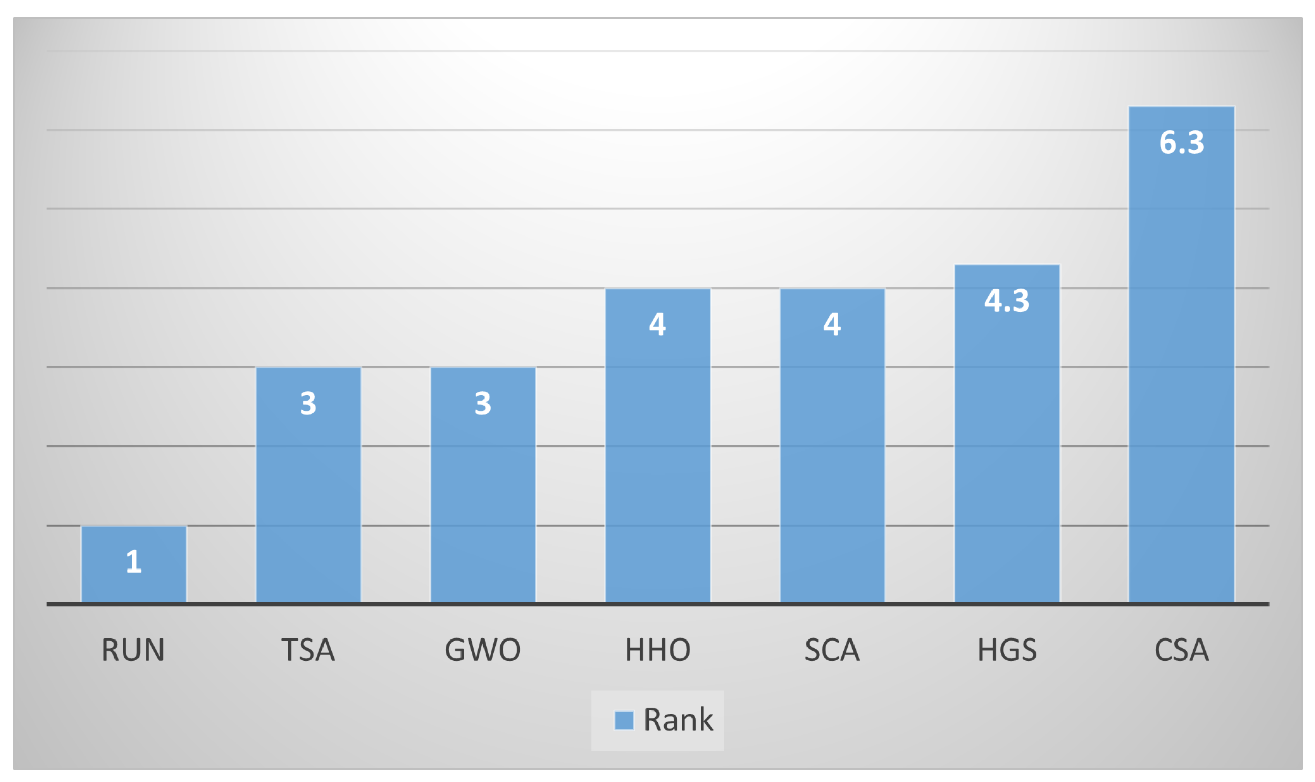
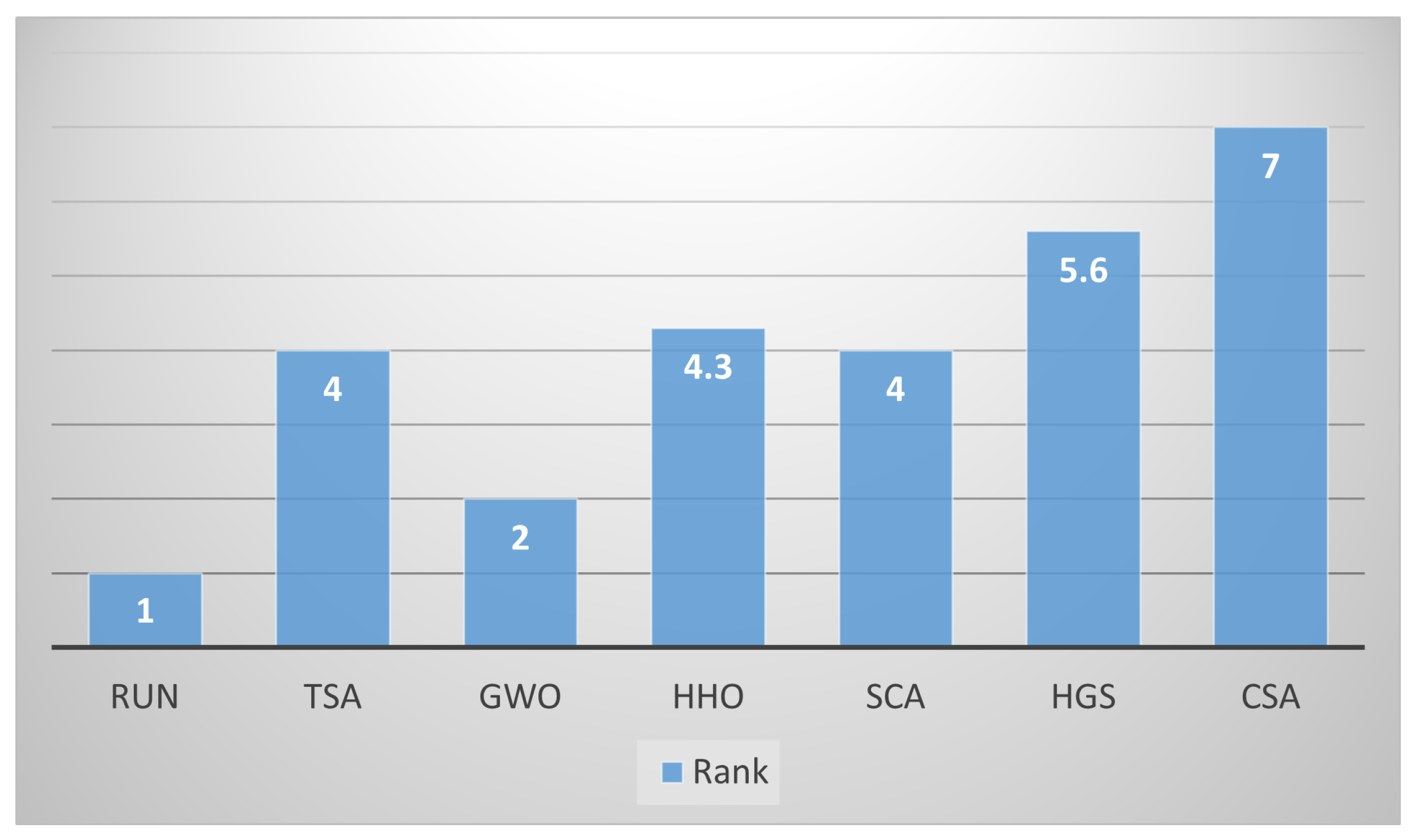
5.4. SDSCM, DDSCM and TDSCM Statistical Analysis

The statistical analysis of all algorithms is performed in this section based on 30 independent runs for all the methods. This analysis is based on calculating the minimum, mean, maximum and standard deviation of the objective function (in this case the RMSE). The algorithm with high accuracy is determined according to the best value of RMSE. The algorithm with more reliability is specified according to the standard deviation of the RMSE value.

Table 6. SDSCM statistical analysis.

Algorithm	SD	Max	Mean	Min
RUN	0.000430699	0.002444572	0.001479894	0.000986242
HGS	0.080450941	0.298406783	0.165531454	0.035316078
TSA	0.006220238	0.033758548	0.006700756	0.002031224
HHO	0.041764534	0.225255019	0.022095052	0.001225477
SCA	0.035145301	0.222879707	0.047425701	0.011590898
CSA	0.191294224	0.528798208	0.347959117	0.002577954
GWO	0.015342251	0.044396167	0.012231984	0.001175457

,

Table 7. DDSCM statistical analysis.

Algorithm	SD	Max	Mean	Min
RUN	0.000514117	0.002947571	0.001481762	0.000987168
HGS	0.073396306	0.311140711	0.172464192	0.06355214
TSA	0.013606881	0.041039694	0.01017202	0.001736175
HHO	0.074681646	0.316600635	0.039488516	0.00120124
SCA	0.03461716	0.222882924	0.046732926	0.01419336
CSA	0.115944599	0.524084107	0.429519392	0.011930562
GWO	0.012659801	0.040747377	0.00909504	0.001149198

and

Table 8. TDSCM statistical analysis.

Algorithm	SD	Max	Mean	Min
RUN	0.001078762	0.006239595	0.001581238	0.000989133
HGS	0.084434623	0.366186646	0.206331896	0.071278042
TSA	0.010155122	0.041606709	0.008013563	0.002362367
HHO	0.088239476	0.308727929	0.053270844	0.001625332
SCA	0.011867222	0.078514615	0.042763328	0.008624898
CSA	0.082428752	0.524789361	0.430931111	0.255247472
GWO	0.007634026	0.034432925	0.006262906	0.00115177

present the statistical analysis of the RUN algorithm and other comparative algorithms for the three models, SDSCM, DDSCM and TDSCM, respectively. Based on these recorded results the proposed RUN algorithm achieves the minimum RMSE and the best value of standard deviation for all SDSCM, SDSCM and TDSCM. Considering this fact, the proposed RUN algorithm is the superior algorithm on all competitor algorithms due to its better reliability and higher accuracy. The robustness and convergence curves of each algorithm are very important items in the evaluation of the performance of algorithms. The robustness curves are explained in Figure 10, Figure 11 and Figure 12 for SDSCM, DDSCM and TDSCM, respectively. These figures explain that the RUN algorithm achieves the best fitness at each run compared with all used algorithms. Considering the above, the proposed RUN algorithm realizes high robustness reliability for the best solution concerning all algorithms. The convergence curves are explained in Figure 13, Figure 14 and Figure 15 for SDSCM, DDSCM and TDSCM, respectively. The convergence curves show how the algorithm behaves along the iterations until reaching the global optimal value of the objective functions. Based on these figures, the proposed RUN algorithm achieves faster convergence to the optimal solution than all algorithms. The Friedman test is a non-parametric statistical test that is used to detect differences in treatments across multiple test attempts. The Friedman rank test is performed for the SDSCM, DDSCM and TDSCM results reported in Table 6, Table 7 and Table 8, respectively. The extension of the Wilcoxon test is the Friedman test. The analysis of the simulated data can be done by using this test. The extracted data of 30 runs for all algorithms is used in measuring the Friedman test for all case studies. Figure 16 presents the Friedman rank for SDSCM. It is observed that RUN obtained the best rank, i.e., rank 1 followed by TSA, GWO, HHO, SCA, HGS and CSA. Figure 17 shows the Friedman rank for DDSCM. It is observed that RUN obtained rank 1 followed by GWO, TSA, HHO, SCA, HGS and CSA. Figure 18 presents the Friedman rank for TDSCM. Here it is observed that RUN obtained the best rank followed by GWO, TSA, SCA, HHO, HGS and CSA. Thus, it can be concluded that RUN obtained the best rank for all the three cases.

Based on the results analysis previously described, the RUN is an optimization mechanism that has been tested over a huge range of real-world problems. However, since it has been recently proposed its performance needs to be proven in different areas of application as energy systems. In this paper the RUN is used to estimate the parameters of solar cells by using three different diode models. The accuracy of the results provided by the RUN helps to verify its performance regarding the optimization. Moreover, the analysis of the results from the application point of view permits to understand that the solar cells designed by the RUN are more efficient in terms of voltage and power. This means that they can be used in real applications due to their capabilities to follow the input design parameters. Besides, the robustness of the RUN is confirmed since the values are stable along different experiments.

The following merits revealed the efficiency of RUN for solving various complex optimization problems:

• In the RUN algorithm, the enhanced solution quality (ESQ) is employed to increase the quality of the solutions and to avoid local optima at each iteration.
• The Scale factor (SF) has a randomized adaptation nature, which assists RUN in further improving the exploration and exploitation steps.
• Using the average position of solutions can promote RUN’s exploration tendency in the early iterations.
• RUN is based on the Runge–Kutta (RK) method; this permits a proper balance between exploration and exploitation.
• The ESQ also helps to promote the quality of solutions and improve the convergence speed.

6. Conclusions and Future Work

In this work, a new optimization technique called Runge–Kutta optimizer (RUN) is applied for the parameter estimation of PV diode models. Comparisons between the RUN algorithm and the Hunger Games Search (HGS) algorithm, the Chameleon Swarm Algorithm (CSA), the Tunicate Swarm Algorithm (TSA), Harris hawk’s optimization (HHO), the Sine–Cosine Algorithm (SCA) and the Grey Wolf Optimization (GWO) algorithm are conducted for the same dataset of R.T.C France solar cells. The performance of the RUN algorithm is compared with all algorithms according to statistical analyses concerning minimum, average, maximum, standard deviation and Friedman rank test of 30 independent runs. The findings show that the closeness between the extracted I-V and P-V curves achieved by the RUN algorithm compared with the measured data is very high. The best RMSE for DDSCM is better than for SDSCM. The TDSCM achieves better RMSE than SDSCM and DDSCM. The performance of robustness and convergence rates is superior for the RUN algorithm for all tested models compared with all competitor algorithms. In future studies, the RUN can be applied for several optimization problems in different fields such as economic load dispatch problem, optimal power flow in power system and estimation of fuel cell parameters.

References

1. Houssein, E.H. Machine Learning and Meta-heuristic Algorithms for Renewable Energy: A Systematic Review. In Advanced Control and Optimization Paradigms for Wind Energy Systems; Springer: Berlin, Germany, 2019; pp. 165–187. [Google Scholar]
2. Ayala, H.V.H.; dos Santos Coelho, L.; Mariani, V.C.; Askarzadeh, A. An improved free search differential evolution algorithm: A case study on parameters identification of one diode equivalent circuit of a solar cell module. Energy 2015, 93, 1515–1522. [Google Scholar] [CrossRef]
3. Zainol Abidin, M.A.; Mahyuddin, M.N.; Mohd Zainuri, M.A.A. Solar Photovoltaic Architecture and Agronomic Management in Agrivoltaic System: A Review. Sustainability 2021, 13, 7846. [Google Scholar] [CrossRef]
4. D’Adamo, I.; Gastaldi, M.; Morone, P. The post COVID-19 green recovery in practice: Assessing the profitability of a policy proposal on residential photovoltaic plants. Energy Policy 2020, 147, 111910. [Google Scholar] [CrossRef]
5. Kim, W.s.; Eom, H.; Kwon, Y. Optimal Design of Photovoltaic Connected Energy Storage System Using Markov Chain Models. Sustainability 2021, 13, 3837. [Google Scholar] [CrossRef]
6. Xu, S.; Wang, Y. Parameter estimation of photovoltaic modules using a hybrid flower pollination algorithm. Energy Convers. Manag. 2017, 144, 53–68. [Google Scholar] [CrossRef]
7. Jordehi, A.R. Enhanced leader particle swarm optimisation (ELPSO): An efficient algorithm for parameter estimation of photovoltaic (PV) cells and modules. Sol. Energy 2018, 159, 78–87. [Google Scholar] [CrossRef]
8. Houssein, E.H.; Mahdy, M.A.; Fathy, A.; Rezk, H. A modified Marine Predator Algorithm based on opposition based learning for tracking the global MPP of shaded PV system. Expert Syst. Appl. 2021, 183, 115253. [Google Scholar] [CrossRef]
9. Houssein, E.H.; Zaki, G.N.; Diab, A.A.Z.; Younis, E.M. An efficient Manta Ray Foraging Optimization algorithm for parameter extraction of three-diode photovoltaic model. Comput. Electr. Eng. 2021, 94, 107304. [Google Scholar] [CrossRef]
10. Mahdavi, S.; Sarhaddi, F.; Hedayatizadeh, M. Energy/exergy based-evaluation of heating/cooling potential of PV/T and earth-air heat exchanger integration into a solar greenhouse. Appl. Therm. Eng. 2019, 149, 996–1007. [Google Scholar] [CrossRef]
11. Houssein, E.H.; Helmy, B.E.d.; Rezk, H.; Nassef, A.M. An enhanced Archimedes optimization algorithm based on Local escaping operator and Orthogonal learning for PEM fuel cell parameter identification. Eng. Appl. Artif. Intell. 2021, 103, 104309. [Google Scholar] [CrossRef]
12. Ismaeel, A.A.; Houssein, E.H.; Oliva, D.; Said, M. Gradient-based optimizer for parameter extraction in photovoltaic models. IEEE Access 2021, 9, 13403–13416. [Google Scholar] [CrossRef]
13. Mostafa, M.; Abdullah, H.M.; Mohamed, M.A. Modeling and Experimental Investigation of Solar Stills for Enhancing Water Desalination Process. IEEE Access 2020, 8, 219457–219472. [Google Scholar] [CrossRef]
14. Alam, D.; Yousri, D.; Eteiba, M. Flower pollination algorithm based solar PV parameter estimation. Energy Convers. Manag. 2015, 101, 410–422. [Google Scholar] [CrossRef]
15. Deb, D.; Brahmbhatt, N.L. Review of yield increase of solar panels through soiling prevention, and a proposed water-free automated cleaning solution. Renew. Sustain. Energy Rev. 2018, 82, 3306–3313. [Google Scholar] [CrossRef]
16. Soliman, M.A.; Hasanien, H.M.; Alkuhayli, A. Marine Predators Algorithm for Parameters Identification of Triple-Diode Photovoltaic Models. IEEE Access 2020, 8, 155832–155842. [Google Scholar] [CrossRef]
17. Qais, M.H.; Hasanien, H.M.; Alghuwainem, S. Parameters extraction of three-diode photovoltaic model using computation and Harris Hawks optimization. Energy 2020, 195, 117040. [Google Scholar] [CrossRef]
18. Qais, M.H.; Hasanien, H.M.; Alghuwainem, S. Transient search optimization for electrical parameters estimation of photovoltaic module based on datasheet values. Energy Convers. Manag. 2020, 214, 112904. [Google Scholar] [CrossRef]
19. Ortiz-Conde, A.; Sánchez, F.J.G.; Muci, J. New method to extract the model parameters of solar cells from the explicit analytic solutions of their illuminated I–V characteristics. Sol. Energy Mater. Sol. Cells 2006, 90, 352–361. [Google Scholar] [CrossRef]
20. Cuce, E.; Cuce, P.M.; Karakas, I.H.; Bali, T. An accurate model for photovoltaic (PV) modules to determine electrical characteristics and thermodynamic performance parameters. Energy Convers. Manag. 2017, 146, 205–216. [Google Scholar] [CrossRef]
21. El Achouby, H.; Zaimi, M.; Ibral, A.; Assaid, E. New analytical approach for modelling effects of temperature and irradiance on physical parameters of photovoltaic solar module. Energy Convers. Manag. 2018, 177, 258–271. [Google Scholar] [CrossRef]
22. Easwarakhanthan, T.; Bottin, J.; Bouhouch, I.; Boutrit, C. Nonlinear minimization algorithm for determining the solar cell parameters with microcomputers. Int. J. Sol. Energy 1986, 4, 1–12. [Google Scholar] [CrossRef]
23. Toledo, F.J.; Blanes, J.M.; Galiano, V. Two-step linear least-squares method for photovoltaic single-diode model parameters extraction. IEEE Trans. Ind. Electron. 2018, 65, 6301–6308. [Google Scholar] [CrossRef]
24. Chegaar, M.; Ouennoughi, Z.; Hoffmann, A. A new method for evaluating illuminated solar cell parameters. Solid-State Electron. 2001, 45, 293–296. [Google Scholar] [CrossRef]
25. Pillai, D.S.; Rajasekar, N. Metaheuristic algorithms for PV parameter identification: A comprehensive review with an application to threshold setting for fault detection in PV systems. Renew. Sustain. Energy Rev. 2018, 82, 3503–3525. [Google Scholar] [CrossRef]
26. Nesmachnow, S. An overview of metaheuristics: Accurate and efficient methods for optimisation. Int. J. Metaheuristics 2014, 3, 320–347. [Google Scholar] [CrossRef]
27. Yang, B.; Wang, J.; Zhang, X.; Yu, T.; Yao, W.; Shu, H.; Zeng, F.; Sun, L. Comprehensive overview of meta-heuristic algorithm applications on PV cell parameter identification. Energy Convers. Manag. 2020, 208, 112595. [Google Scholar] [CrossRef]
28. Yuan, X.; Zhao, J.; Yang, Y.; Wang, Y. Hybrid parallel chaos optimization algorithm with harmony search algorithm. Appl. Soft Comput. 2014, 17, 12–22. [Google Scholar] [CrossRef]
29. Patel, S.J.; Panchal, A.K.; Kheraj, V. Extraction of solar cell parameters from a single current–voltage characteristic using teaching learning based optimization algorithm. Appl. Energy 2014, 119, 384–393. [Google Scholar] [CrossRef]
30. Chen, X.; Yu, K.; Du, W.; Zhao, W.; Liu, G. Parameters identification of solar cell models using generalized oppositional teaching learning based optimization. Energy 2016, 99, 170–180. [Google Scholar] [CrossRef]
31. Fathy, A.; Rezk, H. Parameter estimation of photovoltaic system using imperialist competitive algorithm. Renew. Energy 2017, 111, 307–320. [Google Scholar] [CrossRef]
32. Yu, K.; Liang, J.; Qu, B.; Cheng, Z.; Wang, H. Multiple learning backtracking search algorithm for estimating parameters of photovoltaic models. Appl. Energy 2018, 226, 408–422. [Google Scholar] [CrossRef]
33. Yuan, X.; Yang, Y.; Wang, H. Improved parallel chaos optimization algorithm. Appl. Math. Comput. 2012, 219, 3590–3599. [Google Scholar] [CrossRef]
34. Yuan, X.; Xiang, Y.; He, Y. Parameter extraction of solar cell models using mutative-scale parallel chaos optimization algorithm. Sol. Energy 2014, 108, 238–251. [Google Scholar] [CrossRef]
35. El-Naggar, K.M.; AlRashidi, M.; AlHajri, M.; Al-Othman, A. Simulated annealing algorithm for photovoltaic parameters identification. Sol. Energy 2012, 86, 266–274. [Google Scholar] [CrossRef]
36. Babu, T.S.; Ram, J.P.; Sangeetha, K.; Laudani, A.; Rajasekar, N. Parameter extraction of two diode solar PV model using Fireworks algorithm. Sol. Energy 2016, 140, 265–276. [Google Scholar] [CrossRef]
37. Derick, M.; Rani, C.; Rajesh, M.; Farrag, M.; Wang, Y.; Busawon, K. An improved optimization technique for estimation of solar photovoltaic parameters. Sol. Energy 2017, 157, 116–124. [Google Scholar] [CrossRef]
38. Sadollah, A.; Eskandar, H.; Bahreininejad, A.; Kim, J.H. Water cycle algorithm with evaporation rate for solving constrained and unconstrained optimization problems. Appl. Soft Comput. 2015, 30, 58–71. [Google Scholar] [CrossRef]
39. Pourmousa, N.; Ebrahimi, S.M.; Malekzadeh, M.; Alizadeh, M. Parameter estimation of photovoltaic cells using improved Lozi map based chaotic optimization Algorithm. Sol. Energy 2019, 180, 180–191. [Google Scholar] [CrossRef]
40. Elsheikh, A.; Abd Elaziz, M. Review on applications of particle swarm optimization in solar energy systems. Int. J. Environ. Sci. Technol. 2019, 16, 1159–1170. [Google Scholar] [CrossRef]
41. Ebrahimi, S.M.; Salahshour, E.; Malekzadeh, M.; Gordillo, F. Parameters identification of PV solar cells and modules using flexible particle swarm optimization algorithm. Energy 2019, 179, 358–372. [Google Scholar] [CrossRef]
42. Nunes, H.; Pombo, J.; Mariano, S.; Calado, M.; De Souza, J.F. A new high performance method for determining the parameters of PV cells and modules based on guaranteed convergence particle swarm optimization. Appl. Energy 2018, 211, 774–791. [Google Scholar] [CrossRef]
43. Ma, J.; Man, K.L.; Guan, S.U.; Ting, T.; Wong, P.W. Parameter estimation of photovoltaic model via parallel particle swarm optimization algorithm. Int. J. Energy Res. 2016, 40, 343–352. [Google Scholar] [CrossRef]
44. Dizqah, A.M.; Maheri, A.; Busawon, K. An accurate method for the PV model identification based on a genetic algorithm and the interior-point method. Renew. Energy 2014, 72, 212–222. [Google Scholar] [CrossRef] [Green Version]
45. Jiang, L.L.; Maskell, D.L.; Patra, J.C. Parameter estimation of solar cells and modules using an improved adaptive differential evolution algorithm. Appl. Energy 2013, 112, 185–193. [Google Scholar] [CrossRef]
46. Askarzadeh, A.; Rezazadeh, A. Artificial bee swarm optimization algorithm for parameters identification of solar cell models. Appl. Energy 2013, 102, 943–949. [Google Scholar] [CrossRef]
47. Wang, R.; Zhan, Y.; Zhou, H. Application of artificial bee colony in model parameter identification of solar cells. Energies 2015, 8, 7563–7581. [Google Scholar] [CrossRef]
48. Elazab, O.S.; Hasanien, H.M.; Elgendy, M.A.; Abdeen, A.M. Parameters estimation of single-and multiple-diode photovoltaic model using whale optimisation algorithm. IET Renew. Power Gener. 2018, 12, 1755–1761. [Google Scholar] [CrossRef]
49. Wu, Z.; Yu, D.; Kang, X. Parameter identification of photovoltaic cell model based on improved ant lion optimizer. Energy Convers. Manag. 2017, 151, 107–115. [Google Scholar] [CrossRef]
50. Niu, Q.; Zhang, L.; Li, K. A biogeography-based optimization algorithm with mutation strategies for model parameter estimation of solar and fuel cells. Energy Convers. Manag. 2014, 86, 1173–1185. [Google Scholar] [CrossRef]
51. Kang, T.; Yao, J.; Jin, M.; Yang, S.; Duong, T. A novel improved cuckoo search algorithm for parameter estimation of photovoltaic (PV) models. Energies 2018, 11, 1060. [Google Scholar] [CrossRef] [Green Version]
52. Askarzadeh, A.; dos Santos Coelho, L. Determination of photovoltaic modules parameters at different operating conditions using a novel bird mating optimizer approach. Energy Convers. Manag. 2015, 89, 608–614. [Google Scholar] [CrossRef]
53. Ram, J.P.; Babu, T.S.; Dragicevic, T.; Rajasekar, N. A new hybrid bee pollinator flower pollination algorithm for solar PV parameter estimation. Energy Convers. Manag. 2017, 135, 463–476. [Google Scholar] [CrossRef]
54. Nayak, B.; Mohapatra, A.; Mohanty, K.B. Parameter estimation of single diode PV module based on GWO algorithm. Renew. Energy Focus 2019, 30, 1–12. [Google Scholar] [CrossRef]
55. Awadallah, M.A. Variations of the bacterial foraging algorithm for the extraction of PV module parameters from nameplate data. Energy Convers. Manag. 2016, 113, 312–320. [Google Scholar] [CrossRef]
56. Abbassi, R.; Abbassi, A.; Heidari, A.A.; Mirjalili, S. An efficient salp swarm-inspired algorithm for parameters identification of photovoltaic cell models. Energy Convers. Manag. 2019, 179, 362–372. [Google Scholar] [CrossRef]
57. Gao, X.; Cui, Y.; Hu, J.; Xu, G.; Wang, Z.; Qu, J.; Wang, H. Parameter extraction of solar cell models using improved shuffled complex evolution algorithm. Energy Convers. Manag. 2018, 157, 460–479. [Google Scholar] [CrossRef]
58. Chen, Y.; Chen, Z.; Wu, L.; Long, C.; Lin, P.; Cheng, S. Parameter extraction of PV models using an enhanced shuffled complex evolution algorithm improved by opposition-based learning. Energy Procedia 2019, 158, 991–997. [Google Scholar] [CrossRef]
59. Said, M.; Shaheen, A.M.; Ginidi, A.R.; El-Sehiemy, R.A.; Mahmoud, K.; Lehtonen, M.; Darwish, M.M. Estimating Parameters of Photovoltaic Models Using Accurate Turbulent Flow of Water Optimizer. Processes 2021, 9, 627. [Google Scholar] [CrossRef]
60. Abdelminaam, D.S.; Said, M.; Houssein, E.H. Turbulent Flow of Water-Based Optimization Using New Objective Function for Parameter Extraction of Six Photovoltaic Models. IEEE Access 2021, 9, 35382–35398. [Google Scholar] [CrossRef]
61. Yu, K.; Liang, J.; Qu, B.; Chen, X.; Wang, H. Parameters identification of photovoltaic models using an improved JAYA optimization algorithm. Energy Convers. Manag. 2017, 150, 742–753. [Google Scholar] [CrossRef]
62. Yu, K.; Qu, B.; Yue, C.; Ge, S.; Chen, X.; Liang, J. A performance-guided JAYA algorithm for parameters identification of photovoltaic cell and module. Appl. Energy 2019, 237, 241–257. [Google Scholar] [CrossRef]
63. Yang, Y.; Chen, H.; Heidari, A.A.; Gandomi, A.H. Hunger games search: Visions, conception, implementation, deep analysis, perspectives and towards performance shifts. Expert Syst. Appl. 2021, 177, 114864. [Google Scholar] [CrossRef]
64. Kaur, S.; Awasthi, L.K.; Sangal, A.; Dhiman, G. Tunicate swarm algorithm: A new bio-inspired based metaheuristic paradigm for global optimization. Eng. Appl. Artif. Intell. 2020, 90, 103541. [Google Scholar] [CrossRef]
65. Heidari, A.A.; Mirjalili, S.; Faris, H.; Aljarah, I.; Mafarja, M.; Chen, H. Harris hawks optimization: Algorithm and applications. Future Gener. Comput. Syst. 2019, 97, 849–872. [Google Scholar] [CrossRef]
66. Mirjalili, S. SCA: A sine cosine algorithm for solving optimization problems. Knowl.-Based Syst. 2016, 96, 120–133. [Google Scholar] [CrossRef]
67. Braik, M.S. Chameleon Swarm Algorithm: A bio-inspired optimizer for solving engineering design problems. Expert Syst. Appl. 2021, 174, 114685. [Google Scholar] [CrossRef]
68. Mirjalili, S.; Mirjalili, S.M.; Lewis, A. Grey wolf optimizer. Adv. Eng. Softw. 2014, 69, 46–61. [Google Scholar] [CrossRef] [Green Version]
69. Ahmadianfar, I.; Heidari, A.A.; Gandomi, A.H.; Chu, X.; Chen, H. RUN Beyond the Metaphor: An Efficient Optimization Algorithm Based on Runge–Kutta Method. Expert Syst. Appl. 2021, 181, 115079. [Google Scholar] [CrossRef]
Figure 1. Equivalent circuit of the SDSCM.
Mathematics 09 02313 g001
Figure 2. Equivalent circuit of the DDSCM.
Mathematics 09 02313 g002
Figure 3. Equivalent circuit of the TDSCM.
Mathematics 09 02313 g003
Figure 4. The I-V curve and current absolute error for SDSCM.
Mathematics 09 02313 g004
Figure 5. The P-V curve and power absolute error for SDSCM.
Mathematics 09 02313 g005
Figure 6. The I-V curve and current absolute error for DDSCM.
Mathematics 09 02313 g006
Figure 7. The P-V curve and power absolute error for DDSCM.
Mathematics 09 02313 g007
Figure 8. The I-V curve and current absolute error for TDSCM.
Mathematics 09 02313 g008
Figure 9. The P-V curve and power absolute error for TDSCM.
Mathematics 09 02313 g009
Figure 10. Robustness curve for SDSCM.
Mathematics 09 02313 g010
Figure 11. Robustness curve for DDSCM.
Mathematics 09 02313 g011
Figure 12. Robustness curve for TDSCM.
Mathematics 09 02313 g012
Figure 13. Convergence curve for SDSCM.
Mathematics 09 02313 g013
Figure 14. Convergence curve for DDSCM.
Mathematics 09 02313 g014
Figure 15. Convergence curve for TDSCM.
Mathematics 09 02313 g015
Figure 16. Friedman rank curve for SDSCM.
Mathematics 09 02313 g016
Figure 17. Friedman rank curve for DDSCM.
Mathematics 09 02313 g017
Figure 18. Friedman rank curve for TDSCM.
Mathematics 09 02313 g018