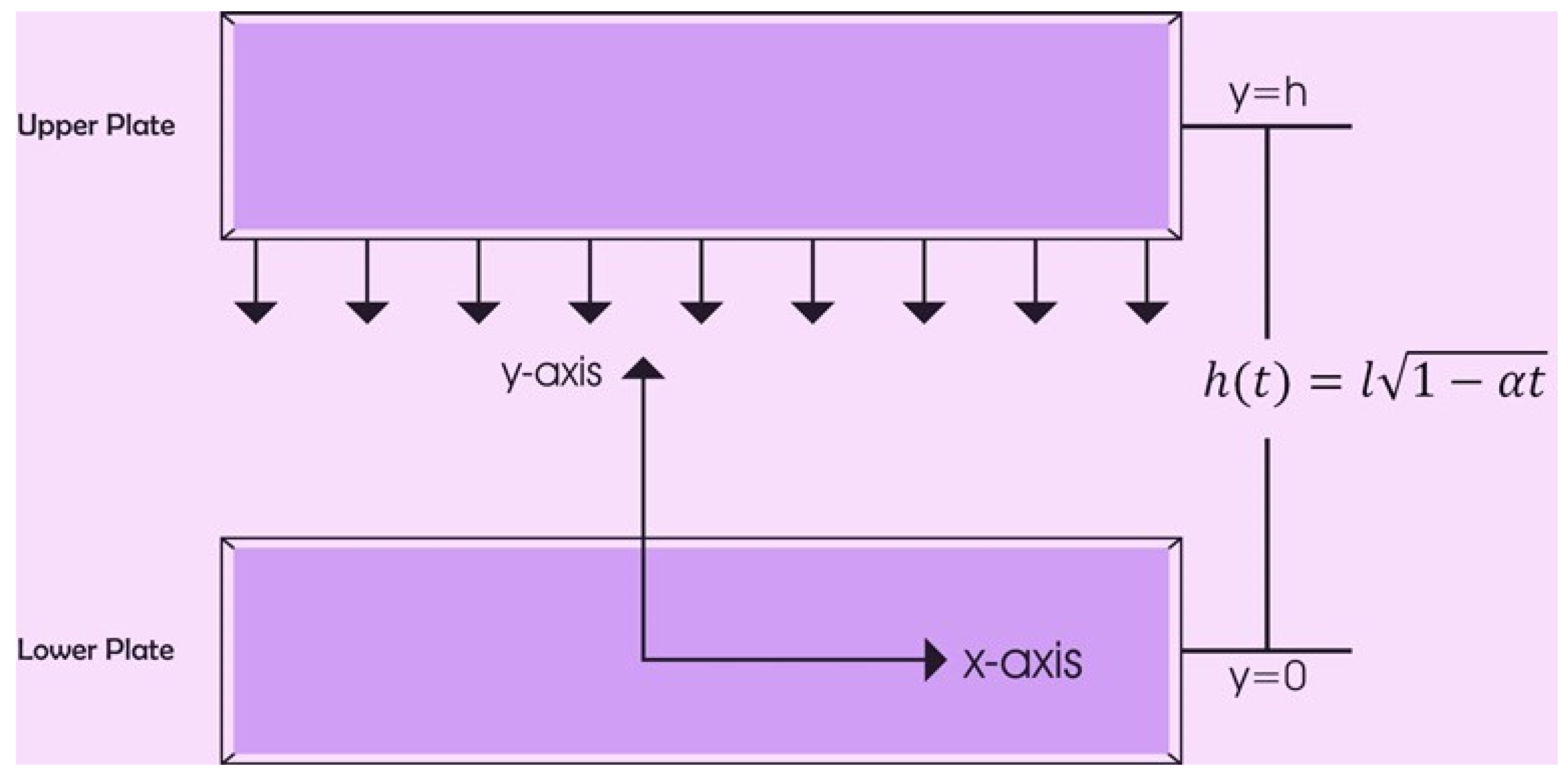
Figure 1.
Geometry of the Problem.
Figure 1.
Geometry of the Problem.
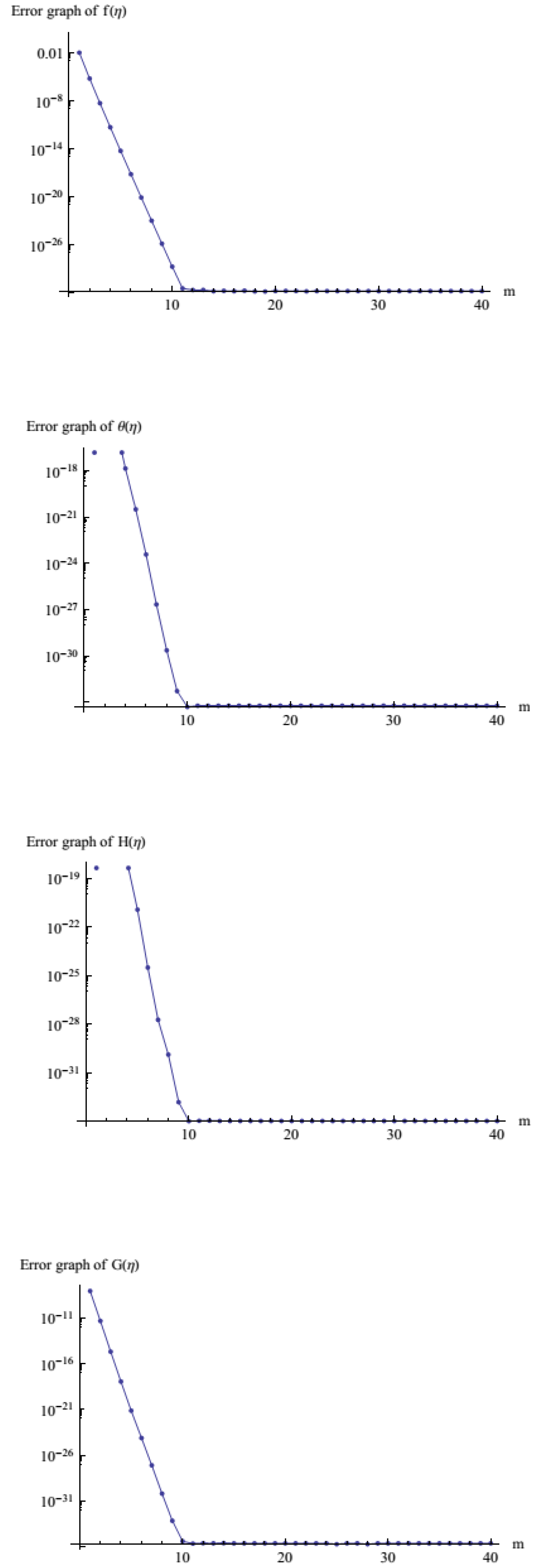
Figure 2.
Illustration of the error profiles of , , and with fixed values of , , , , , , , , and .
Figure 2.
Illustration of the error profiles of , , and with fixed values of , , , , , , , , and .
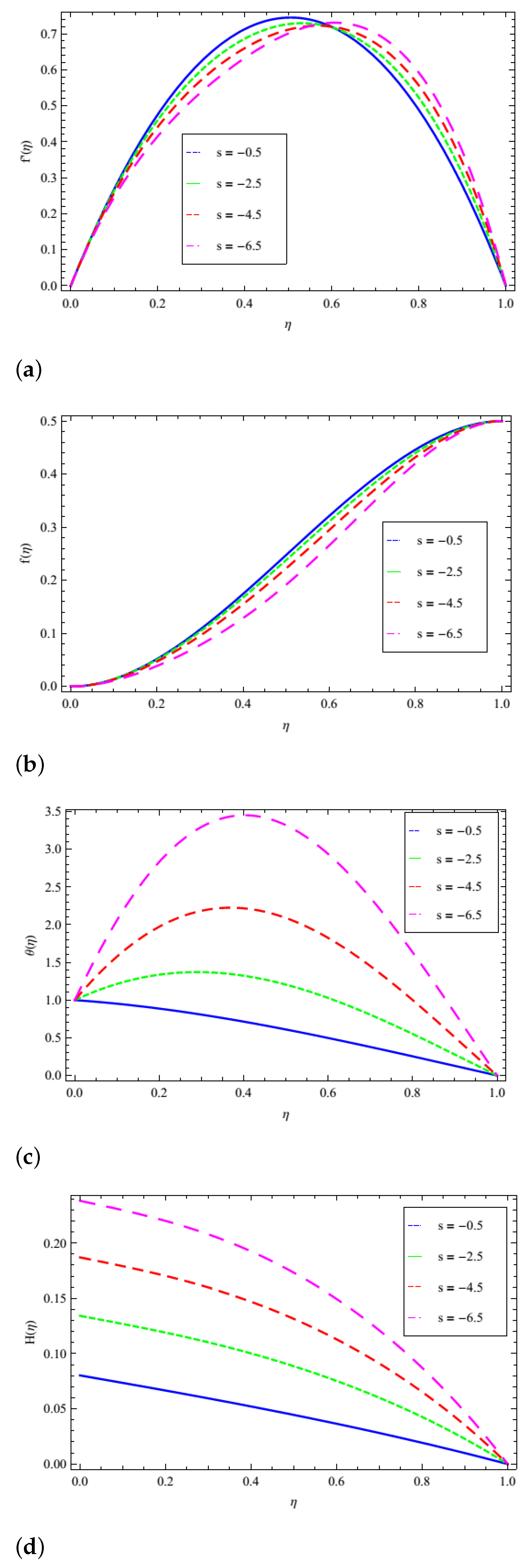
Figure 3.
Impact of S on (a) velocity component along y-axis , (b) velocity component along x-axis , (c) heat distribution variable and (d) homogeneous reaction for the specific values , , , , , , .
Figure 3.
Impact of S on (a) velocity component along y-axis , (b) velocity component along x-axis , (c) heat distribution variable and (d) homogeneous reaction for the specific values , , , , , , .
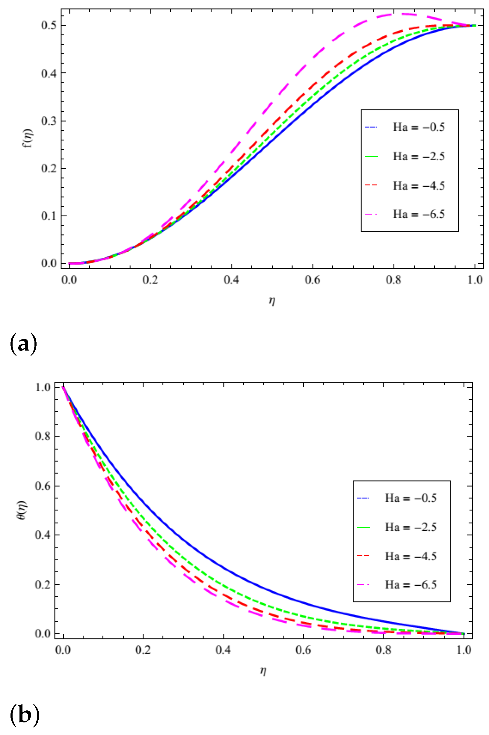
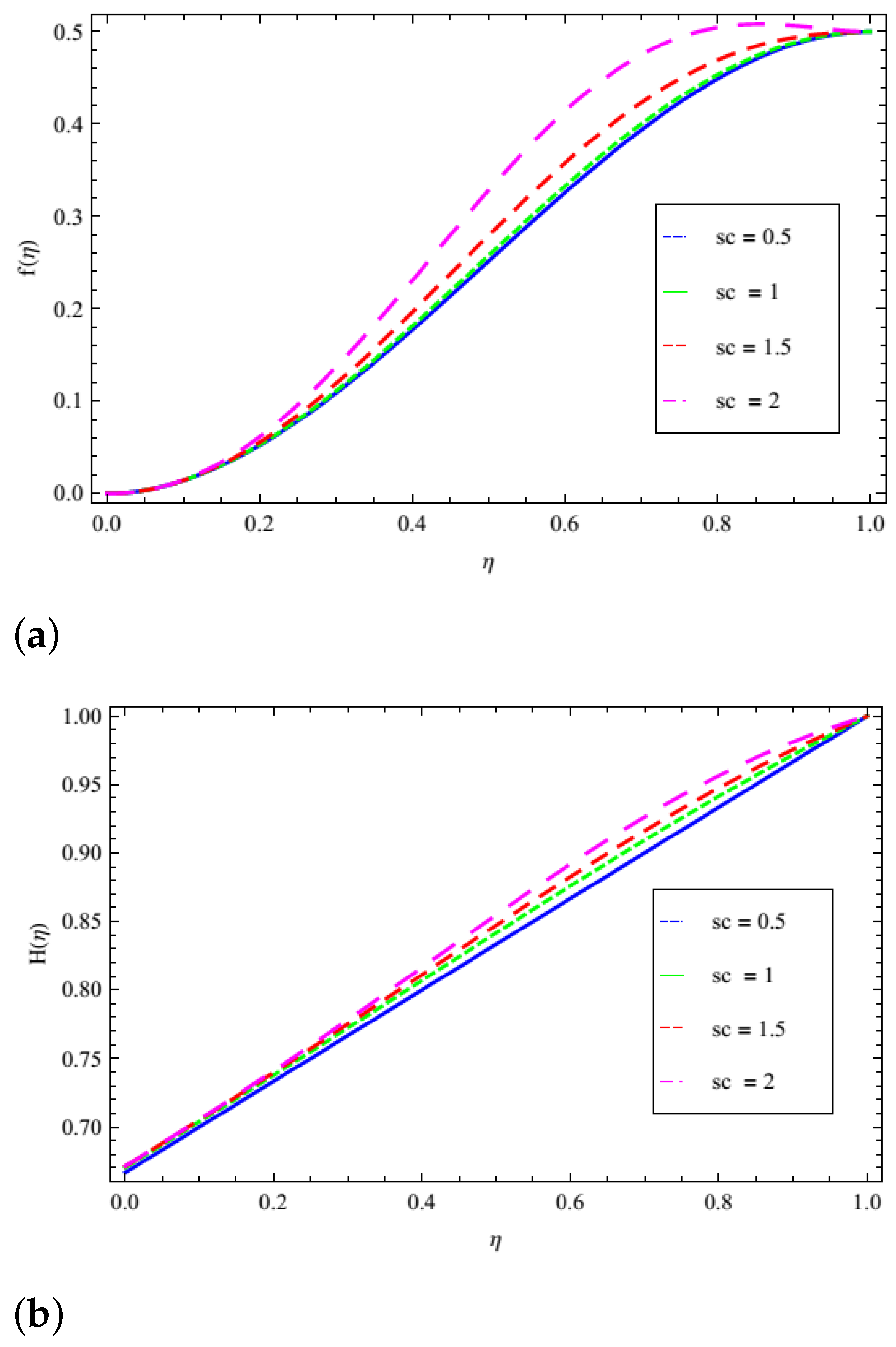
Figure 4.
Impact of on (a) velocity component and (b) heat distribution variable for specific values , , , , .
Figure 4.
Impact of on (a) velocity component and (b) heat distribution variable for specific values , , , , .
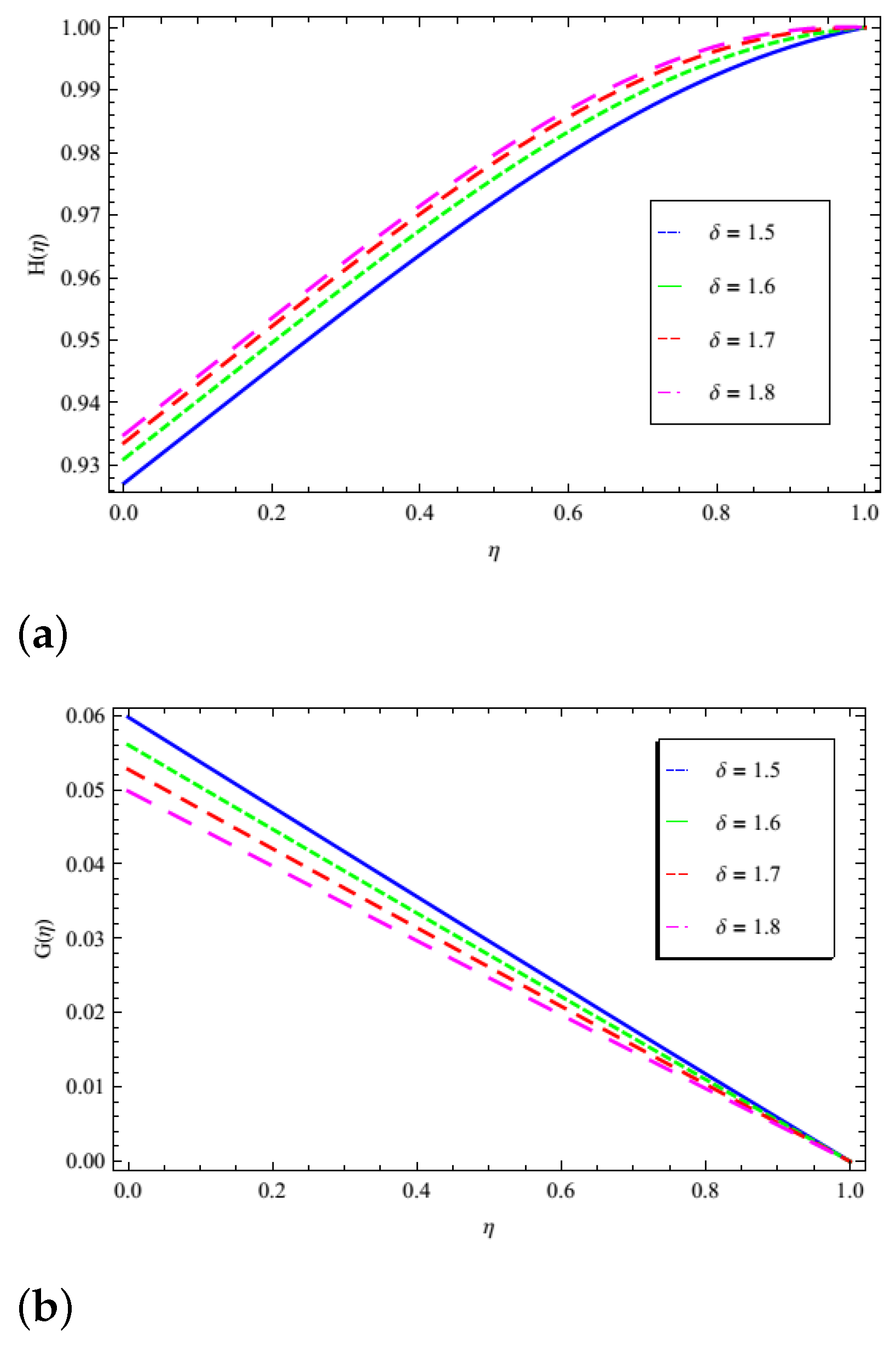
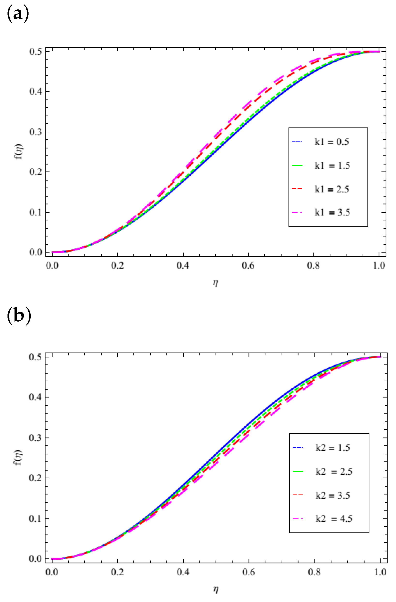
Figure 5.
Impact of on (a) homogeneous reaction and (b) heterogeneous reaction for specific values , , , .
Figure 5.
Impact of on (a) homogeneous reaction and (b) heterogeneous reaction for specific values , , , .
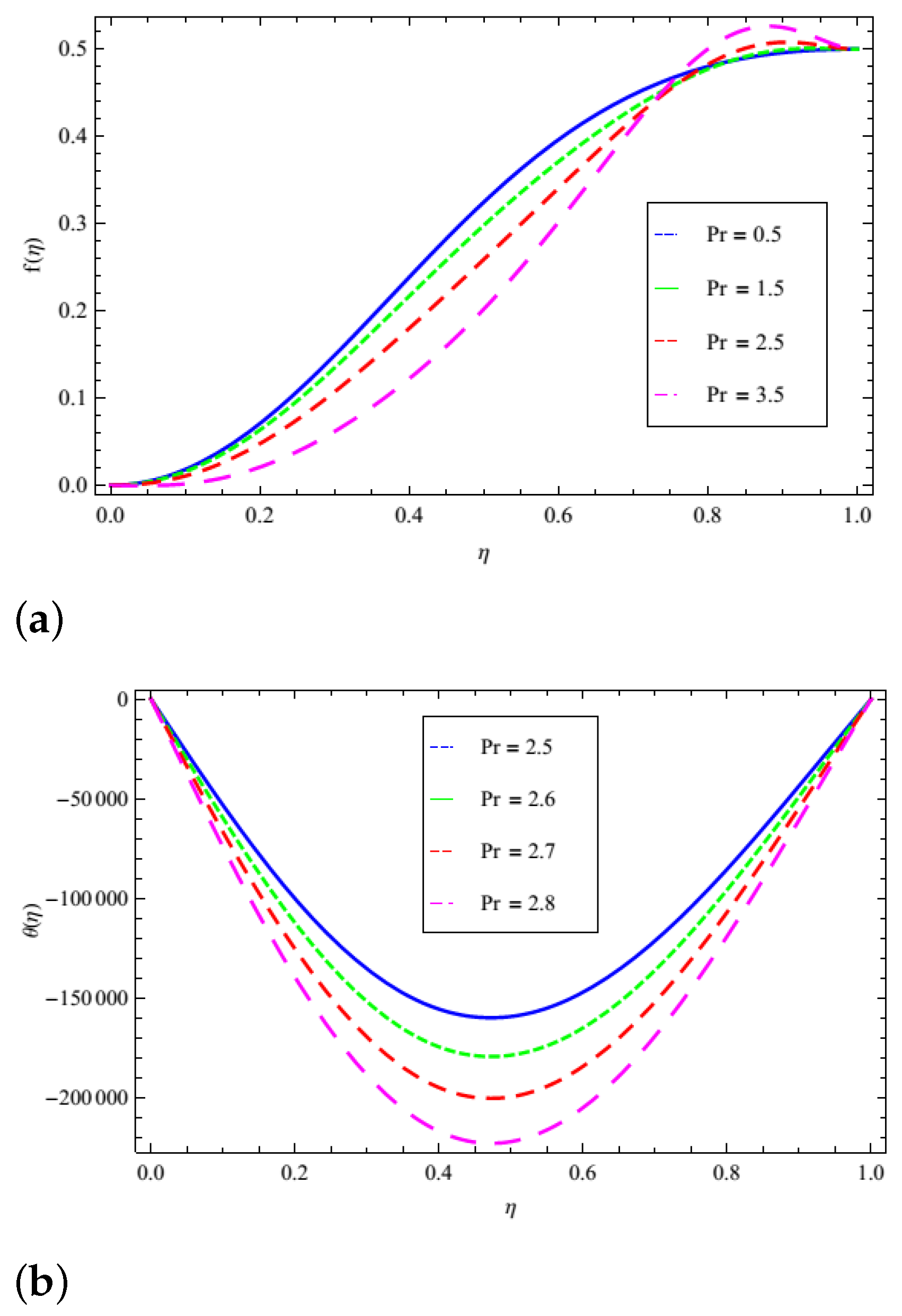
Figure 6.
Impact of on (a) velocity component along x-axis and (b) heat distribution variable for specific values , , , , .
Figure 6.
Impact of on (a) velocity component along x-axis and (b) heat distribution variable for specific values , , , , .
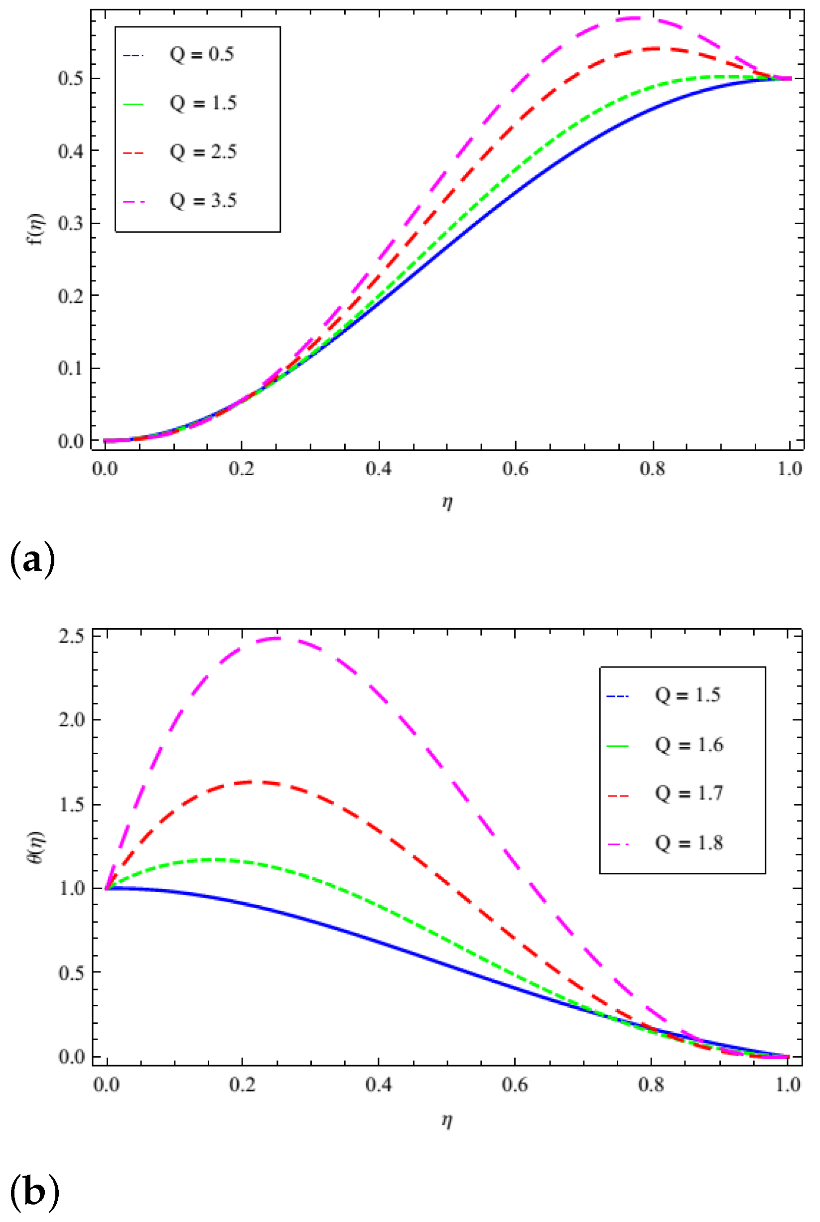
Figure 7.
Impact of Q on (a) velocity component along x-axis and (b) heat distribution variable for specific values , , , , .
Figure 7.
Impact of Q on (a) velocity component along x-axis and (b) heat distribution variable for specific values , , , , .
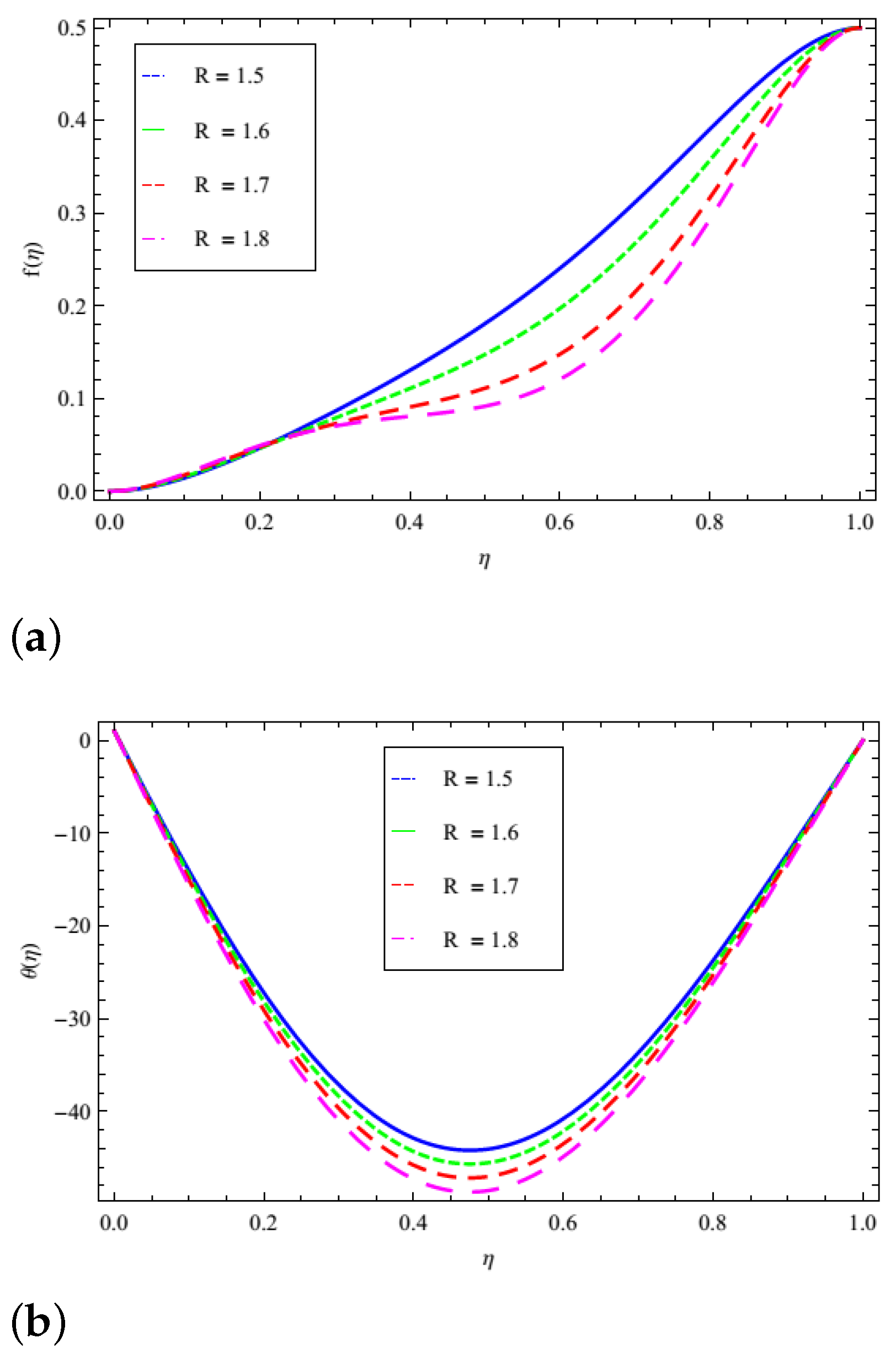
Figure 8.
Impact of R on (a) velocity component along x-axis and (b) heat distribution variable for specific values , , , , , .
Figure 8.
Impact of R on (a) velocity component along x-axis and (b) heat distribution variable for specific values , , , , , .
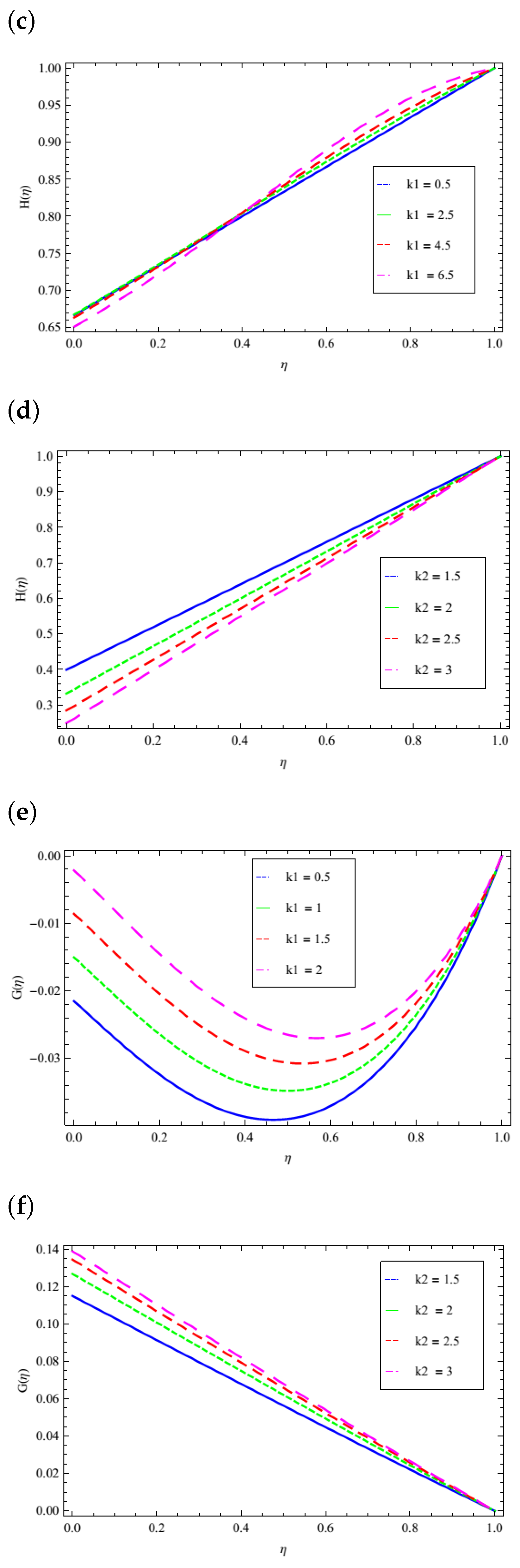
Figure 9.
Illustration of the impact of (a) on , (b) on , (c) on , (d) on , (e) on and (f) on for specific values , , , , , , .
Figure 9.
Illustration of the impact of (a) on , (b) on , (c) on , (d) on , (e) on and (f) on for specific values , , , , , , .
Figure 10.
Impact of on (a) velocity component and (b) homogeneous reaction for specific values , , , , , , .
Figure 10.
Impact of on (a) velocity component and (b) homogeneous reaction for specific values , , , , , , .
Table 1.
Total residual error of , , and with fixed values of , , , , , , .
Table 1.
Total residual error of , , and with fixed values of , , , , , , .
| m | | | | |
|---|
| 1 | | | | |
| 5 | | | | |
| 10 | | | | |
| 15 | | | | |
| 20 | | | | |
| 25 | | | | |
| 30 | | | | |
| 33 | | | | |
| 37 | | | | |
| 40 | | | | |
Table 2.
Convergence of the homotopy solution for differing orders of calculation for , , and when , , , .
Table 2.
Convergence of the homotopy solution for differing orders of calculation for , , and when , , , .
| | | | |
|---|
| 0 | | | | |
| | | | |
| | | | |
| | | | |
| | | | |
| | | | |
| | | | |
| | | | |
| | | | |
| | | | |
| 1 | | | | |
Table 3.
Computations for , , and when , , , and various values of . Furthermore, and
Table 3.
Computations for , , and when , , , and various values of . Furthermore, and
| HAM Result | Numerical Result |
|---|
| | | | | | | |
|---|
| 0 | 0 | 1 | | | 0 | 1 | | |
| | | | | | | | |
| | | | | | | | |
| | | | | | | | |
| | | | | | | | |
| | | | | | | | |
| | | | | | | | |
| | | | | | | | |
| | | | | | | | |
| | | | | | | | |
| 1 | | A | 1 | B | | | | 0 |
Table 4.
Computational for , , and with , , and differing values of S.
Table 4.
Computational for , , and with , , and differing values of S.
| S | HAM Result | BVP4c Result |
|---|
| | | | | | | |
|---|
| | | | | | | | |
| | | | | | | | |
| | | | | | | | |
| | | | | | | | |
Table 5.
Computational for , , and with , , , and differing values of .
Table 5.
Computational for , , and with , , , and differing values of .
| HAM Result | Numerical Result |
|---|
| | | | | | | |
|---|
| | | | | | | | |
| 1 | | | | | | | | |
| | | | | | | | |
| 2 | | | | | | | | |
Table 6.
Computational for , , and with , , , and differing values of .
Table 6.
Computational for , , and with , , , and differing values of .
| D | HAM Result | Numerical Result |
|---|
| | | | | | | |
|---|
| 1 | | | | | | | | |
| 2 | | | | | | | | |
| 3 | | | | | | | | |
| 4 | | | | | | | | |
Table 7.
Computational for , , and with , , , and differing values of .
Table 7.
Computational for , , and with , , , and differing values of .
| HAM Result | Numerical Result |
|---|
| | | | | | | |
|---|
| 1 | | | | | | | | |
| 2 | | | | | | | | |
| 3 | | | | | | | | |
| 4 | | | | | | | | |
Table 8.
Computational for , , and with , , and differing values of Q.
Table 8.
Computational for , , and with , , and differing values of Q.
| Q | HAM Result | Numerical Result |
|---|
| | | | | | | |
|---|
| 1 | | | | | | | | |
| 2 | | | | | | | | |
| 3 | | | | | | | | |
| 4 | | | | | | | | |
Table 9.
Computational for , , and with , , , and differing values of R.
Table 9.
Computational for , , and with , , , and differing values of R.
| R | HAM Result | Numerical Result |
|---|
| | | | | | | |
|---|
| | | | | | | | |
| | | | | | | | |
| | | | | | | | |
| | | | | | | | |
Table 10.
Computational for , , and with , , , and differing values of .
Table 10.
Computational for , , and with , , , and differing values of .
| HAM Result | Numerical Result |
|---|
| | | | | | | |
|---|
| | | | | | | | |
| | | | | | | | |
| | | | | | | | |
| | | | | | | | |
Table 11.
Computational for , , and with , , , and differing values of .
Table 11.
Computational for , , and with , , , and differing values of .
| HAM Result | Numerical Result |
|---|
| | | | | | | |
|---|
| | | | | | | | |
| 1 | | | | | | | | |
| 2 | | | | | | | | |
| 3 | | | | | | | | |
Table 12.
Computational for , , and with , , , and differing values of .
Table 12.
Computational for , , and with , , , and differing values of .
| HAM Result | Numerical Result |
|---|
| | | | | | | |
|---|
| | | | | | | | |
| 1 | | | | | | | | |
| 2 | | | | | | | | |
| 3 | | | | | | | | |


 ,
, 


