Large Deformation Problem of Bimodular Functionally-Graded Thin Circular Plates Subjected to Transversely Uniformly-Distributed Load: Perturbation Solution without Small-Rotation-Angle Assumption

Abstract

In this study, the large deformation problem of a functionally-graded thin circular plate subjected to transversely uniformly-distributed load and with different moduli in tension and compression (bimodular property) is theoretically analyzed, in which the small-rotation-angle assumption, commonly used in the classical Föppl–von Kármán equations of large deflection problems, is abandoned. First, based on the mechanical model on the neutral layer, the bimodular functionally-graded property of materials is modeled as two different exponential functions in the tensile and compressive zones. Thus, the governing equations of the large deformation problem are established and improved, in which the equation of equilibrium is derived without the common small-rotation-angle assumption. Taking the central deflection as a perturbation parameter, the perturbation method is used to solve the governing equations, thus the perturbation solutions of deflection and stress are obtained under different boundary constraints and the regression of the solution is satisfied. Results indicate that the perturbation solutions presented in this study have higher computational accuracy in comparison with the existing perturbation solutions with small-rotation-angle assumption. Specially, the computational accuracies of external load and yield stress are improved by 17.22% and 28.79% at most, respectively, by the numerical examples. In addition, the small-rotation-angle assumption has a great influence on the yield stress at the center of the bimodular functionally-graded circular plate.

1. Introduction

The elastic large deformation problem of flexible thin plates has been a focus of attention for scholars all over the world. Because of its strong geometrical nonlinearity, it is generally difficult to establish the effective governing equations used for the solution to the problem. For a long time, the classical Föppl–von Kármán equation has been used to describe the large deflection behavior of thin plates; however, the influence caused by small-rotation-angle assumption commonly used in the derivation of the equation has always been ignored. In some real applications, the deflection magnitude is moderate, while the rotation angle of the plate may achieve a relatively large value, which makes investigation into small-rotation-angle assumption inevitable.

In addition to the geometrical nonlinearity caused by the elastic large deformation problem, the materials that constitute flexible plates also present some nonlinear problems that cannot be solved by the original methods used for elastic, isotropic, and homogeneous materials, for example, functionally graded material (FGM) with different properties in tension and compression. Therefore, the nonlinearity of materials, in combination with the geometrical nonlinearity from the large deformation problem, brings about many topics of interest for the engineering and academic professions. In this study, we will theoretically analyze the elastic large deformation problem of a bimodular functionally-graded thin circular plate, and further use perturbation methods to obtain an asymptotic solution. For this purpose, the review for existing works will begin with the bimodular problem, followed by the functionally-graded material problems, the bimodular functionally-graded material problems, and last, the large deformation problem, giving up the small-rotation-angle assumption as well as the corresponding solving method.

The bimodular problem seems not to be well-known but, in reality, has a long history. Many works have indicated that most materials, including graphite, plastics, steel concrete, ceramics, powder metallurgy materials, polymeric materials, and some composites exhibit different tensile and compressive strains when they bear the same stress applied in tension or compression [1,2]. Therefore, these materials exhibit different moduli of elasticity in tension and compression, and they are known as bimodular materials [3,4]. Basically, there are two models used in the academic analysis in the field of engineering. Bert [5] proposed the model based on the criterion of positive-negative signs in the longitudinal strain of fibers, which is mainly applicable to orthotropic materials and, as a result, a large amount of related works concerning laminated composites have emerged [6,7,8,9,10]. Bruno et al. [6] investigated bimodular composite plates under compression. Using the higher-order finite strip method, Tseng and Lee [7] analyzed the bending of bimodular laminates. Zinno and Greco [8] investigated the damage evolution in bimodular laminated composite under cyclic loading. Using higher-order shear deformation theory, Ganapathi et al. [9] analyzed the static problem of bimodular laminated composite plates subjected to mechanical loads. Khan and Patel [10] investigated the nonlinear periodic response of bimodular laminated composite annular sector plates. Another model that is established on the criterion of positive-negative signs of principal stress was proposed by Ambartsumyan [11], and this model is mainly used for isotropic materials. In structural engineering, the stress state along certain principal directions is a key issue during the stress analysis for some structural elements such as beams and plates, because it is this factor that determines whether the point is tensile or compressive. Due to the fact that this bimodular theory founds its constitutive model on principal directions, generally, the principal stress is finally obtained as a result but not as a known condition in advance, which incurs inevitable difficulties from the description of the stress state of a point. At the same time, this model also lacks the ability to describe the experimental data of elastic constants in the complex states of stress. There are a few analytical solutions that concern beams and plates only [12,13,14,15,16]. Yao and Ye [12] derived the analytical solution of a bending bimodular beam subject to lateral force. Applying the equivalent section method, He et al. [13] solved the same problem. Zhao and Ye [14] obtained the analytical elasticity solution of bimodular beams under combined loads. Thereafter, He et al. [15] derived an analytical solution of bending thin plates with bimodular effect, and then He et al. [16] derived the general perturbation solution of a large-deflection circular plate with bimodular effect under various edge conditions. For some complex problems, researchers had to resort to the finite element method (FEM), based on an iterative technique [17,18,19,20,21,22]. Zhang and Wang [17] first proposed the FEM of the elasticity problem with different moduli in tension and compression. Ye et al. [18] reviewed the progresses in elasticity theory with bimodular effect and related FEM. Thereafter, Sun et al. [19] reviewed the mechanical problems with bimodular effect and pointed out that, due to the inherent complexity of the constitutive relation, an FEM based on iterative strategy was required. Gao et al. [20] investigated the temperature stress of a bimodular beam placed on a Winkler foundation, and Ma et al. [21] studied the nonlinear large deflection buckling of compression rod with different moduli. In their numerical simulations, the FEM iterative procedure was used. To overcome convergence difficulties and other disadvantages of traditional iterative methods, Du et al. [22] established an efficient computational framework for the solution of boundary value problems involving bimodular materials.

In recent decades, the issues related to FGM have become an important research topic in many engineering and technical fields, such as aerospace [23], civil engineering [24], acoustics [25], and micro-electro-mechanical systems [26]. FGMs are new types of composite material, which are composed of two or more materials, such as alloy and ceramic, and the composition of these two (or more) materials presents continuous gradient changes [27]. There are many works on structural elements made of FGM, most of them dealing with beams and plates, for example, Nguyen et al. [28]. Among the studies, few studies consider the bimodular property of FGM. As indicated above, most materials will present bimodular properties, which can be obvious or not; thus, FGM seems to be no exception.

More recently, the bimodular property of materials has been gradually introduced into the analysis field of FGM and structures. There are also a few works concerning bimodular FGM beam and plate problems [29,30,31]. Focusing on bimodular FGM plates, He et al. [30] established the simplified theory based on a neutral layer under small-deflection; thereafter, He et al. [31] derived the governing equations of the large-deflection problem of bimodular FGM thin circular plate. However, consideration of geometrical nonlinearity seems to be insufficient. As indicated above, for the large deformation problem of thin plates, not only the deflection of the plate but also the rotation angle presents a relatively large value, and the two factors cannot be ignored.

The definition of the small-rotation-angle assumption means the rotation, β, of the deformed thin plate is so small that it satisfies the approximate relationship sinβ ≈ tanβ. In fact, because sinβ is equal to 1/[1 + 1/tan²β]^1/2 and is not equal to tanβ, no matter how small the rotation is, the small-rotation-angle assumption would inevitably bring an error to the solution of the large-deflection problem of thin plates. Moreover, with the increase of the transversely uniformly-distributed load applied on the surface of the plate, the rotation of the thin plate will increase, and the error caused by the small-rotation-angle assumption increase accordingly. Therefore, in order to eliminate the influence of the small-rotation-angle assumption on the computational accuracy of the solution of the large deformation problem, we need to re-examine this mechanical problem by using the basic relationship between sinβ and tanβ to replace the original approximate relationship. That is to say, we will solve a large deformation problem based on large-deflection and give up the small-rotation-angle assumption.

As for the solving method, the classical perturbation technique will be followed to solve the established governing equations. Generally speaking, there are two advantages for this technique: one advantage is that we can easily obtain the relationship of load vs. central deflection if the central deflection is selected as a perturbation parameter; another may be from the asymptotic characteristics that the perturbation method itself has. In the past, there have been many successful examples of the application of perturbation in the solving of flexible thin plate. Groundbreaking works may be found in Vincent [32] and Chien [33], in which Vincent adopted the load, whereas Chien adopted the central deflection as a perturbation parameter to successfully solve the large-deflection problem of thin plates. Subsequent researchers focused mainly on the choice of perturbation parameters, for example, a generalized displacement [34], a linear function of Poisson’s ratio [35], and an average angular deflection [36]. Chen and Kuang [37] discussed the differences among the possible perturbation parameters.

On the other hand, the magnitude of the perturbation parameter is an important issue that we must face during the perturbation. According to the classical works by Nayfeh [38], perturbation parameters are small parameters; however, this small parameter does not mean the central deflection is also small. Generally speaking, in light of the magnitude of the ratio of the central deflection to plate thickness, if the ratio is less than 1/5, the behavior of the plate may be regarded as rigid, in which the bending effect is dominant and the small-deflection theory is appropriate. If the ratio is greater than 5, the behavior of the plate may be regarded as an absolute flexible plate, or membrane, and the corresponding membrane theory in which the tensile effect is dominant should be adopted in this case. If the ratio falls into the range of 1/5 to 5, the behavior of the plate may be analyzed by the large-deflection theory, which was founded by Föppl–von Kármán. In our study, the ratio is limited in the range of 1/5 to 4, which obviously belongs to the large-deflection problems, although the parameter used for the perturbation attributes to a small parameter. In our next perturbation, the perturbation parameter does not have to be far less than 1, and in some cases it may be far greater than 1. This fact may also be found in many previous studies, including Chien’s pioneer work [39] and, later, Shen’s review [40], in which the perturbation parameter may be greater than 1 and reaches 4–5 in the post-buckling problems of plates.

Besides the choice and magnitude of perturbation parameters mentioned above, there have been many studies concerning the number and physical meaning of the parameter selected. Given that the application of this method does not belong to our study emphasis, we do not review them in detail.

In this study, the perturbation method is used to solve the large deformation problem of a bimodular FGM thin circular plate, with the emphasis on the influence of a small-rotation-angle assumption on the final results. This paper is arranged as follows. In Section 2, the governing equation of the studied problem is established, in which the equation of equilibrium is derived without small-rotation-angle assumption. In Section 3, taking the central deflection as a perturbation parameter, the perturbation solutions of stress and deflection are obtained, and the yield stress under large deformation is also analyzed. In Section 4, the influences of the small-rotation-angle assumption on the relationship of loads vs. central deflection and on the yield stress are discussed in detail. Section 5 is the concluding remarks.

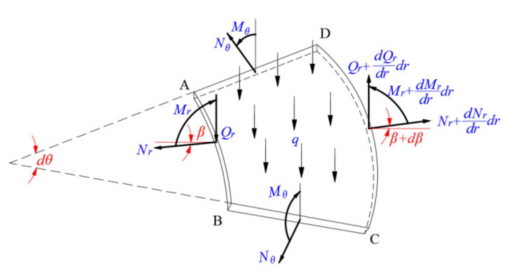
2. Governing Equations and Boundary Conditions

2.1. Establishment of Governing Equations

A bimodular FGM thin circular plate with thickness t and radius a is subjected to a transversely uniformly-distributed load, q, as shown in Figure 1, where the dot-dash line at the peripheral of the plate represents the location of the unknown neutral layer of the plate; this location will be determined later. The polar coordinates plane (r, ϕ) of the cylindrical coordinates system (r, ϕ, z) is established on the plane where the neutral layer is located; r, ϕ, and z represent the radial, circumferential, and transverse coordinates, respectively. Due to the axisymmetric characteristics, ϕ is not presented in Figure 1; t₁ and t₂ represent the height of the tensile and compressive zones, respectively, and the corresponding modulus in the two zones is the tensile modulus, E⁺(z), and compressive modulus, E⁻(z), respectively, as shown in Figure 1. In addition, the special constraint on the plate is not provided initially, as we will solve the problem under multiple constraints.

For the obtainment of an explicit solution of the problem, we need to define the mathematical form of the bimodular FGM model first. Considering the convenience of differential and integral operations, we model E⁺(z) and E⁻(z) as the following exponent type functions [30,31]

$$E^{+}(z)=E_0{e}^{{\alpha }_{1}z/t},\hspace{0.33em}{E}^{-}(z)=E_0{e}^{{\alpha }_{2}z/t},$$

(1)

where α₁ and α₂ are the two graded indices in tensile and compressive zones, and E₀ denotes the Young’s modulus of elasticity on the neutral layer. From Equation (1), it is easy to see that E⁺(z) = E⁻(z) = E₀ when α₁ = α₂ = 0 or z = 0. The bimodular property of FGM is thus simulated mathematically. At the same time, because the influence of Poisson’s ratio on the deformation and stress is much less than that of Young’s modulus of elasticity, Poisson ratios may be assumed as two constants, υ⁺ and υ⁻, neglecting the change along the z direction.

Let us take a differential element, ABCD, from the deformed circular plate to study the static equilibrium problem of this element, as shown in Figure 2, where surfaces AD and BC are located along the radial direction, while surfaces AB and DC are located along the circumferential direction. In Figure 2, N_r and N_θ are the radial and circumferential forces, respectively, M_r and M_θ are the radial and circumferential bending moments, respectively, Q_r is the transverse shear force acting on surfaces AB and DC, dθ denotes the angle between the radial surfaces AD and BC, and β denotes the rotation of the radial force. Note that, due to axisymmetric characteristics, there is no increment from surface AD to surface BC, while the increment will take place from surface AB to surface DC due to the change of r.

The usually so-called in-plane equilibrium equation is [41]

$$\frac{\mathrm{d}}{\mathrm{d}r}\left(r{N}_r\right)-N_{\theta }=0,$$

(2)

where the body force of the plate is neglected. The equation of equilibrium along the vertical direction perpendicular to the polar coordinates plane can be written as

$$\begin{array}{l}\left(N_r+\frac{\mathrm{d}{N}_r}{\mathrm{d}r}\mathrm{d}r\right)(r+\mathrm{d}r)\mathrm{d}\theta \left(\sin \beta +\frac{\mathrm{d}\sin \beta }{\mathrm{d}r}\mathrm{d}r\right)-N_{r}r\mathrm{d}\theta \sin \beta \\ +\left(Q_r+\frac{\mathrm{d}{Q}_r}{\mathrm{d}r}\mathrm{d}r\right)(r+\mathrm{d}r)\mathrm{d}\theta -Q_{r}r\mathrm{d}\theta -\frac{q\left[{(r+\mathrm{d}r)}^2\mathrm{d}\theta -r^2\mathrm{d}\theta \right]}{2}=0\end{array}$$

(3)

where the body force of the plate is also neglected. After ignoring the third order and fourth order differential items of Equation (3), we have

$$\begin{array}{l}r\frac{\mathrm{d}{N}_r}{\mathrm{d}r}\mathrm{d}r\mathrm{d}\theta \sin \beta +N_r\mathrm{d}r\mathrm{d}\theta \sin \beta +r{N}_r\mathrm{d}\theta \frac{\mathrm{d}\sin \beta }{\mathrm{d}r}\mathrm{d}r\\ +r\frac{\mathrm{d}{Q}_r}{\mathrm{d}r}\mathrm{d}r\mathrm{d}\theta +Q_r\mathrm{d}r\mathrm{d}\theta -qr\mathrm{d}r\mathrm{d}\theta =0.\end{array}$$

(4)

Dividing Equation (4) by drdθ yields

$$\frac{\mathrm{d}}{\mathrm{d}r}\left(r{N}_r\sin \beta \right)+\frac{\mathrm{d}}{\mathrm{d}r}\left(r{Q}_r\right)-qr=0,$$

(5)

where

$$\sin \beta =1/\sqrt{1+1/{\tan }^2\beta }=-\frac{\mathrm{d}w}{\mathrm{d}r}{\left[1+{\left(-\frac{\mathrm{d}w}{\mathrm{d}r}\right)}^2\right]}^{-1/2}.$$

(6)

The basic relationship of trigonometric functions is adopted in Equation (6) to replace the original small-rotation-angle assumption that the rotation, β, of the deformed thin plate is so small that sinβ ≈ tanβ holds true.

At the same time, the equation of equilibrium of the moment of the differential element ABCD can be expressed as

$$\left(M_r+\frac{\mathrm{d}{M}_r}{\mathrm{d}r}\mathrm{d}r\right)\left(r+\mathrm{d}r\right)\mathrm{d}\theta -M_{r}r\mathrm{d}\theta -2M_{\theta }\mathrm{d}r\sin \frac{\mathrm{d}\theta }{2}+\left(Q_r+\frac{\mathrm{d}{Q}_r}{\mathrm{d}r}\mathrm{d}r\right)\left(r+\mathrm{d}r\right)\mathrm{d}\theta \mathrm{d}r=0.$$

(7)

After ignoring the third order and fourth order differential items and dividing by drdθ, Equation (7) can be simplified as

$$\frac{\mathrm{d}}{\mathrm{d}r}\left(r{M}_r\right)-M_{\theta }+r{Q}_r=0.$$

(8)

Substituting rQ_r in Equation (8) into Equation (5) yields

$$\frac{\mathrm{d}}{\mathrm{d}r}\left\{-r{N}_r\frac{\mathrm{d}w}{\mathrm{d}r}{\left[1+{\left(-\frac{\mathrm{d}w}{\mathrm{d}r}\right)}^2\right]}^{-1/2}\right\}-\frac{{\mathrm{d}}^2}{\mathrm{d}{r}^2}\left(r{M}_r\right)+\frac{\mathrm{d}{M}_{\theta }}{\mathrm{d}r}-qr=0.$$

(9)

Suppose that the displacements of the neutral layer along the r and z directions are u and w, respectively, and the radii of the radial and circumferential curvatures of the neutral layer are ρ_r and ρ_θ, respectively. The strain components of any point at the z axis in the plate come from two different aspects, one is the tensile strain on the neutral layer and another from the bending strain; that is [31]

$$\epsilon ={\epsilon }_0+z{\epsilon }_1,$$

(10)

where

$$\epsilon ={\left\{{\epsilon }_r,{\epsilon }_{\theta }\right\}}^T,\hspace{1em}{\epsilon }_0={\left\{{\epsilon }_{r0},{\epsilon }_{\theta 0}\right\}}^T,\hspace{1em}{\epsilon }_1={\left\{{\epsilon }_{r1},{\epsilon }_{\theta 1}\right\}}^T,$$

(11)

$${\epsilon }_0={\left\{\frac{\mathrm{d}u}{\mathrm{d}r}+\frac{1}{2}{\left(\frac{\mathrm{d}w}{\mathrm{d}r}\right)}^2,\frac{u}{r}\right\}}^T,\hspace{1em}{\epsilon }_1={\left\{\frac{1}{{\rho }_r},\frac{1}{{\rho }_{\theta }}\right\}}^T.$$

(12)

We note that, in the small-deflection theory as well as the common large-deflection theory of plate, the approximate expressions of the radial curvature and circumferential curvatures is 1/ρ_r = −d²w/dr² and 1/ρ_θ = −(dw/dr)/r, respectively. They are now replaced with the following exact expressions [33]:

$$\left\{\begin{array}{l}\frac{1}{{\rho }_r}=-\frac{{\mathrm{d}}^{2}w}{\mathrm{d}{r}^2}{\left[1+{\left(-\frac{\mathrm{d}w}{\mathrm{d}r}\right)}^2\right]}^{-3/2}\\ \frac{1}{{\rho }_{\theta }}=\frac{1}{r}\sin \beta =-\frac{1}{r}\frac{\mathrm{d}w}{\mathrm{d}r}{\left[1+{\left(-\frac{\mathrm{d}w}{\mathrm{d}r}\right)}^2\right]}^{-1/2}\end{array}\right..$$

(13)

Suppose that the radial and circumferential stresses in the tensile and compressive zones is ${\sigma }_r^{+/-}$ and ${\sigma }_{\theta }^{+/-}$, respectively. The strain-stress relations give [30]

$$\left\{\begin{array}{l}{\sigma }_r^{+/-}=\frac{E^{+/-}(z)}{1-{({\nu }^{+/-})}^2}({\epsilon }_r+\nu {\epsilon }_{\theta })\\ {\sigma }_{\theta }^{+/-}=\frac{E^{+/-}(z)}{1-{({\nu }^{+/-})}^2}({\epsilon }_{\theta }+\nu {\epsilon }_r)\end{array}\right..$$

(14)

Substituting Equations (10)–(12) into Equation (14), it is found that

$$\left\{\begin{array}{l}{\sigma }_r^{+/-}=\frac{E^{+/-}(z)}{1-{({\nu }^{+/-})}^2}\left[\frac{\mathrm{d}u}{\mathrm{d}r}+\frac{1}{2}{\left(\frac{\mathrm{d}w}{\mathrm{d}r}\right)}^2+{\nu }^{+/-}\frac{u}{r}+z\left(\frac{1}{{\rho }_r}+{\nu }^{+/-}\frac{1}{{\rho }_{\theta }}\right)\right]\\ {\sigma }_{\theta }^{+/-}=\frac{E^{+/-}(z)}{1-{({\nu }^{+/-})}^2}\left[\frac{u}{r}+{\nu }^{+/-}\frac{\mathrm{d}u}{\mathrm{d}r}+\frac{{\nu }^{+/-}}{2}{\left(\frac{\mathrm{d}w}{\mathrm{d}r}\right)}^2+z\left(\frac{1}{{\rho }_{\theta }}+{\nu }^{+/-}\frac{1}{{\rho }_r}\right)\right]\end{array}\right..$$

(15)

The radial and circumferential bending moments, M_r and M_θ, may be expressed, in terms of the radial stress and circumferential stress [31], as

$$\left\{\begin{array}{l}{M}_r={\displaystyle {\int }_0^{t_1}{\sigma }_r^{+}z}\mathrm{d}z+{\displaystyle {\int }_{-t_2}^0{\sigma }_r^{-}}z\mathrm{d}z\\ M_{\theta }={\displaystyle {\int }_0^{t_1}{\sigma }_{\theta }^{+}}z\mathrm{d}z+{\displaystyle {\int }_{-t_2}^0{\sigma }_{\theta }^{-}z}\mathrm{d}z\end{array}\right..$$

(16)

Substituting Equation (15) into Equation (16) yields

$$\left\{\begin{array}{c}{M}_r=A_1^{+}\left[\frac{\mathrm{d}u}{\mathrm{d}r}+\frac{1}{2}{\left(\frac{\mathrm{d}w}{\mathrm{d}r}\right)}^2+{\nu }^{+}\frac{u}{r}\right]+A_2^{+}\left(\frac{1}{{\rho }_r}+\frac{{\nu }^{+}}{{\rho }_{\theta }}\right)\hfill \\ +A_1^{-}\left[\frac{\mathrm{d}u}{\mathrm{d}r}+\frac{1}{2}{\left(\frac{\mathrm{d}w}{\mathrm{d}r}\right)}^2+{\nu }^{-}\frac{u}{r}\right]+A_2^{-}\left(\frac{1}{{\rho }_r}+\frac{{\nu }^{-}}{{\rho }_{\theta }}\right)\hfill \\ M_{\theta }=A_1^{+}\left[\frac{u}{r}+{\nu }^{+}\frac{\mathrm{d}u}{\mathrm{d}r}+{\nu }^{+}\frac{1}{2}{\left(\frac{\mathrm{d}w}{\mathrm{d}r}\right)}^2\right]+A_2^{+}\left(\frac{1}{{\rho }_{\theta }}+{\nu }^{+}\frac{1}{{\rho }_r}\right)\hfill \\ +A_1^{-}\left[\frac{u}{r}+{\nu }^{+}\frac{\mathrm{d}u}{\mathrm{d}r}+{\nu }^{-}\frac{1}{2}{\left(\frac{\mathrm{d}w}{\mathrm{d}r}\right)}^2\right]+A_2^{-}\left(\frac{1}{{\rho }_{\theta }}+{\nu }^{-}\frac{1}{{\rho }_r}\right)\hfill \end{array}\right.,$$

(17)

where

$$\left\{\begin{array}{c}{A}_1^{+}=\frac{{\int }_0^{t_1}z{E}_0{e}^{{\alpha }_{1}z/t}\mathrm{d}z}{1-{\left({\nu }^{+}\right)}^2}=\frac{1}{1-{\left({\nu }^{+}\right)}^2}\left[\frac{E_0{t}^2}{{\alpha }_1^2}+\left(\frac{t_{1}t}{{\alpha }_1}-\frac{t^2}{{\alpha }_1^2}\right)E_0{e}^{{\alpha }_1{t}_1/t}\right]\hfill \\ A_1^{-}=\frac{{\int }_{-t_2}^{0}z{E}_0{e}^{{\alpha }_{2}z/t}\mathrm{d}z}{1-{\left({\nu }^{-}\right)}^2}=\frac{1}{1-{\left({\nu }^{-}\right)}^2}\left[-\frac{E_0{t}^2}{{\alpha }_2^2}+\left(\frac{t_{2}t}{{\alpha }_2}+\frac{t^2}{{\alpha }_2^2}\right)E_0{e}^{-{\alpha }_2{t}_2/t}\right]\hfill \\ A_2^{+}=\frac{{\int }_0^{t_1}{z}^2{E}_0{e}^{{\alpha }_{1}z/t}\mathrm{d}z}{1-{\left({\nu }^{+}\right)}^2}=\frac{1}{1-{\left({\nu }^{+}\right)}^2}\left[\left(\frac{2t^3}{{\alpha }_1^3}+\frac{t_1^{2}t}{{\alpha }_1}-\frac{2t^2{t}_1}{{\alpha }_1^2}\right)E_0{e}^{{\alpha }_1{t}_1/t}-\frac{2E_0{t}^3}{{\alpha }_1^3}\right]\hfill \\ A_2^{-}=\frac{{\int }_{-t_2}^0{z}^2{E}_0{e}^{{\alpha }_{2}z/t}\mathrm{d}z}{1-{\left({\nu }^{-}\right)}^2}=\frac{1}{1-{\left({\nu }^{-}\right)}^2}\left[-\left(\frac{2t^3}{{\alpha }_2^3}+\frac{t_2^{2}t}{{\alpha }_2}+\frac{2t^2{t}_2}{{\alpha }_2^2}\right)E_0{e}^{-{\alpha }_2{t}_2/t}+\frac{2E_0{t}^3}{{\alpha }_2^3}\right]\hfill \end{array}\right..$$

(18)

The integral of the items containing z in Equation (18) should be determined as zero, i.e., $A_1^{+}$ + $A_1^{-}$ = 0, because it is exactly the condition used for determining the position of the unknown neutral layer in [31]. Thus, the expressions of M_r and M_θ can be further rewritten as

$$\left\{\begin{array}{l}{M}_r=A_2^{+}\left(\frac{1}{{\rho }_r}+\frac{{\nu }^{+}}{{\rho }_{\theta }}\right)+A_2^{-}\left(\frac{1}{{\rho }_r}+\frac{{\nu }^{-}}{{\rho }_{\theta }}\right)\\ M_{\theta }=A_2^{+}\left(\frac{1}{{\rho }_{\theta }}+\frac{{\nu }^{+}}{{\rho }_r}\right)+A_2^{-}\left(\frac{1}{{\rho }_{\theta }}+\frac{{\nu }^{-}}{{\rho }_r}\right)\end{array}\right..$$

(19)

Substituting Equation (19) into Equation (9), we may obtain the governing equation of the bimodular FGM thin circular plates without small-rotation-angle assumption, as follows

$$\begin{array}{l}{D}^{\ast }\frac{{\mathrm{d}}^2}{\mathrm{d}{r}^2}\left\{r\frac{{\mathrm{d}}^{2}w}{\mathrm{d}{r}^2}{\left[1+{\left(-\frac{\mathrm{d}w}{\mathrm{d}r}\right)}^2\right]}^{-3/2}\right.\left.+{\nu }^{+/-}\frac{\mathrm{d}w}{\mathrm{d}r}{\left[1+{\left(-\frac{\mathrm{d}w}{\mathrm{d}r}\right)}^2\right]}^{-1/2}\right\}\\ -D^{\ast }\frac{\mathrm{d}}{\mathrm{d}r}\left\{\frac{1}{r}\frac{\mathrm{d}w}{\mathrm{d}r}{\left[1+{\left(-\frac{\mathrm{d}w}{\mathrm{d}r}\right)}^2\right]}^{-1/2}\right.\left.+{\nu }^{+/-}\frac{{\mathrm{d}}^{2}w}{\mathrm{d}{r}^2}{\left[1+{\left(-\frac{\mathrm{d}w}{\mathrm{d}r}\right)}^2\right]}^{-3/2}\right\}\\ +\frac{\mathrm{d}}{\mathrm{d}r}\left\{-r{N}_r\frac{\mathrm{d}w}{\mathrm{d}r}{\left[1+{\left(-\frac{\mathrm{d}w}{\mathrm{d}r}\right)}^2\right]}^{-1/2}\right\}-qr=0\end{array}$$

(20)

where D* = $A_2^{+}$ + $A_2^{-}$. To differentiate Equation (20) from the common Föppl–von Kármán equation, we name it the improved Föppl–von Kármán equation without small-rotation-angle assumption.

The radial force, N_r, and circumferential force, N_θ, are the sum of integrals in the tensile zone and the compressive zone, such that [31]

$$\left\{\begin{array}{l}{N}_r={\displaystyle {\int }_0^{t_1}{\sigma }_r^{+}}\mathrm{d}z+{\displaystyle {\int }_{-t_2}^0{\sigma }_r^{-}}\mathrm{d}z\\ N_{\theta }={\displaystyle {\int }_0^{t_1}{\sigma }_{\theta }^{+}}\mathrm{d}z+{\displaystyle {\int }_{-t_2}^0{\sigma }_{\theta }^{-}}\mathrm{d}z\end{array}\right..$$

(21)

After substituting Equation (15) into Equation (21), N_r and N_θ are rewritten as

$$\left\{\begin{array}{l}{N}_r=A_3\left[\frac{\mathrm{d}u}{\mathrm{d}r}+\frac{1}{2}{\left(\frac{\mathrm{d}w}{\mathrm{d}r}\right)}^2+{\nu }^{+}\frac{u}{r}\right]\\ N_{\theta }=A_3\left[\frac{u}{r}+{\nu }^{+}\frac{\mathrm{d}u}{\mathrm{d}r}+{\nu }^{+}\frac{1}{2}{\left(\frac{\mathrm{d}w}{\mathrm{d}r}\right)}^2\right]\end{array}\right.,$$

(22)

where

$$A_3=\frac{{\displaystyle {\int }_{-t_2}^{t_1}{E}^{+}(z)}dz}{1-{({\nu }^{+})}^2}=\frac{{\displaystyle {\int }_{-t_2}^{t_1}{E}_0{e}^{{\alpha }_{1}z/t}dz}}{1-{({\nu }^{+})}^2}=\frac{1}{1-{({\nu }^{+})}^2}\frac{E_{0}t}{{\alpha }_1}\left(\frac{e^{{\alpha }_1}-1}{e^{{\alpha }_1{t}_2/t}}\right).$$

(23)

It should be mentioned that, in the large-deflection problem of plate, any point of the plate is stretched along the radial and circumferential directions, so all integrals along the thickness direction should be performed only on the tensile components. Besides, the integrals of the items containing z are also equal to zero in Equation (21). From Equations (2) and (22), we have

$$\frac{u}{r}=\frac{1}{A_3}(N_{\theta }-{\nu }^{+}{N}_r)=\frac{1}{A_3}\left[\frac{\mathrm{d}}{\mathrm{d}r}(r{N}_r)-{\nu }^{+}{N}_r\right].$$

(24)

Substituting u in Equation (24) into the first formula of Equation (22), we have

$$r\frac{\mathrm{d}}{\mathrm{d}r}\left[\frac{1}{r}\frac{\mathrm{d}}{\mathrm{d}r}\left(r^2{N}_r\right)\right]+\frac{A_3}{2}{\left(\frac{\mathrm{d}w}{\mathrm{d}r}\right)}^2=0.$$

(25)

Equation (25) is the compatible equation of the large deformation problem of the bimodular FGM thin circular plate. Lastly, the improved equilibrium relation (Equation (20)), in combination with the compatible relation (Equation (25)), constitute the governing equations of the problem.

2.2. Verification of Regression and Simplification of Equations

Next, we will verify that Equation (20) can be regressed to the classical Föppl–von Kármán equation. If the mechanical properties of different modulus and FGM effect are not taken into account, the bending stiffness of the bimodular FGM thin plate D^* is regressed to the bending stiffness of the isotropic plate D. The limit of D^* when α₁, α₂→0 is

$$\begin{array}{l}\underset{{\alpha }_1,{\alpha }_2\to 0}{\lim }{D}^{\ast }=\underset{{\alpha }_1,{\alpha }_2\to 0}{\lim }\frac{E_0}{1-{({\nu }^{+})}^2}\left[\left(\frac{2t^3}{{\alpha }_1^3}+\frac{t_1^{2}t}{{\alpha }_1}-\frac{2t^2{t}_1}{{\alpha }_1^2}\right)e^{{\alpha }_1{t}_1/t}-\frac{2t^3}{{\alpha }_1^3}\right]\\ +\frac{E_0}{1-{({\nu }^{-})}^2}\left[-\left(\frac{2t^3}{{\alpha }_2^3}+\frac{t_2^{2}t}{{\alpha }_2}+\frac{2t^2{t}_2}{{\alpha }_2^2}\right)e^{-{\alpha }_2{t}_2/t}+\frac{2t^3}{{\alpha }_2^3}\right]=\frac{E_0{t}_1^3}{3\left[1-{({\nu }^{+})}^2\right]}+\frac{E_0{t}_2^3}{3\left[1-{({\nu }^{-})}^2\right]}.\end{array}$$

(26)

Because t₁ = t₂ = t/2 when α₁ = α₂ = 0 and υ⁺ = υ⁻ = υ, the bending stiffness of isotropic and homogeneous plate can be obtained

$$D=\underset{\begin{array}{l}{\alpha }_1,{\alpha }_2\to 0\\ {\nu }^{+}={\nu }^{-}=\nu \end{array}}{\lim }{D}^{\ast }=\frac{E_0{t}^3}{12\left(1-{\nu }^2\right)}.$$

(27)

Besides, when the term 1 + (−dw/dr)² in Equation (20) is approximately equal to 1, Equation (20) may be further simplified as

$$D\left(\frac{{\mathrm{d}}^{4}w}{\mathrm{d}{r}^4}+\frac{2}{r}\frac{{\mathrm{d}}^{3}w}{\mathrm{d}{r}^3}-\frac{1}{r^2}\frac{{\mathrm{d}}^{2}w}{\mathrm{d}{r}^2}+\frac{1}{r^3}\frac{\mathrm{d}w}{\mathrm{d}r}\right)=q+\frac{1}{r}{N}_r\frac{\mathrm{d}w}{\mathrm{d}r}+N_r\frac{{\mathrm{d}}^{2}w}{\mathrm{d}{r}^2}+\frac{\mathrm{d}{N}_r}{\mathrm{d}r}\frac{\mathrm{d}w}{\mathrm{d}r},$$

(28)

which is the classical Föppl–von Kármán equation in the case of large-deflection. The satisfaction of regression indicates that the improved governing equation in large deformation may regress to the classical Föppl–von Kármán equation in large-deflection.

Note that there are many nonlinear items concerning 1 + (−dw/dr)² in Equation (20), which further makes its solving complicated; therefore, moderate simplification is necessary. For this purpose, the denominator terms in Equation (20) are expanded in the form of the power series with respect to (−dw/dr)², such that

$${\left[1+{\left(-\frac{\mathrm{d}w}{\mathrm{d}r}\right)}^2\right]}^{-3/2}=1-\frac{3}{2}{\left(-\frac{\mathrm{d}w}{\mathrm{d}r}\right)}^2+\frac{15}{8}{\left(-\frac{\mathrm{d}w}{\mathrm{d}r}\right)}^4-\frac{35}{16}{\left(-\frac{\mathrm{d}w}{\mathrm{d}r}\right)}^6+\dots$$

(29)

and

$${\left[1+{\left(-\frac{\mathrm{d}w}{\mathrm{d}r}\right)}^2\right]}^{-1/2}=1-\frac{1}{2}{\left(-\frac{\mathrm{d}w}{\mathrm{d}r}\right)}^2+\frac{3}{8}{\left(-\frac{\mathrm{d}w}{\mathrm{d}r}\right)}^4-\frac{5}{16}{\left(-\frac{\mathrm{d}w}{\mathrm{d}r}\right)}^6+\dots .$$

(30)

Substituting the first and second terms of Equations (29) and (30) into Equation (20), we have

$$\begin{array}{l}{D}^{\ast }\frac{{\mathrm{d}}^2}{\mathrm{d}{r}^2}\left\{r\frac{{\mathrm{d}}^{2}w}{\mathrm{d}{r}^2}\left[1-\frac{3}{2}{\left(-\frac{\mathrm{d}w}{\mathrm{d}r}\right)}^2\right]\right.\left.+{\nu }^{+/-}\frac{\mathrm{d}w}{\mathrm{d}r}\left[1-\frac{1}{2}{\left(-\frac{\mathrm{d}w}{\mathrm{d}r}\right)}^2\right]\right\}\\ -D^{\ast }\frac{\mathrm{d}}{\mathrm{d}r}\left\{\frac{1}{r}\frac{\mathrm{d}w}{\mathrm{d}r}\left[1-\frac{1}{2}{\left(-\frac{\mathrm{d}w}{\mathrm{d}r}\right)}^2\right]\right.\left.+{\nu }^{+/-}\frac{{\mathrm{d}}^{2}w}{\mathrm{d}{r}^2}\left[1-\frac{3}{2}{\left(-\frac{\mathrm{d}w}{\mathrm{d}r}\right)}^2\right]\right\}\\ +\frac{\mathrm{d}}{\mathrm{d}r}\left\{-r{N}_r\frac{\mathrm{d}w}{\mathrm{d}r}\left[1-\frac{1}{2}{\left(-\frac{\mathrm{d}w}{\mathrm{d}r}\right)}^2\right]\right\}-qr=0.\end{array}$$

(31)

Integrating Equation (31) yields

$$\begin{array}{l}{D}^{\ast }\frac{\mathrm{d}}{\mathrm{d}r}\left\{r\frac{{\mathrm{d}}^{2}w}{\mathrm{d}{r}^2}\left[1-\frac{3}{2}{\left(-\frac{\mathrm{d}w}{\mathrm{d}r}\right)}^2\right]\right.\left.+{\nu }^{+/-}\frac{\mathrm{d}w}{\mathrm{d}r}\left[1-\frac{1}{2}{\left(-\frac{\mathrm{d}w}{\mathrm{d}r}\right)}^2\right]\right\}\\ -D^{\ast }\left\{\frac{1}{r}\frac{\mathrm{d}w}{\mathrm{d}r}\left[1-\frac{1}{2}{\left(-\frac{\mathrm{d}w}{\mathrm{d}r}\right)}^2\right]\right.\left.+{\nu }^{+/-}\frac{{\mathrm{d}}^{2}w}{\mathrm{d}{r}^2}\left[1-\frac{3}{2}{\left(-\frac{\mathrm{d}w}{\mathrm{d}r}\right)}^2\right]\right\}\\ =\frac{1}{2}q{r}^2+r{N}_r\frac{\mathrm{d}w}{\mathrm{d}r}\left[1-\frac{1}{2}{\left(-\frac{\mathrm{d}w}{\mathrm{d}r}\right)}^2\right]+C.\end{array}$$

(32)

It can be seen that C = 0 according to the boundary conditions dw/dr = 0 and N_r ≠ 0 at r = 0. The items containing υ^+/− are then all offset by calculating the first derivation in Equation (32), and the simplified equilibrium equation is now

$$\begin{array}{l}{D}^{\ast }\left\{r\frac{{\mathrm{d}}^{3}w}{\mathrm{d}{r}^3}+\frac{{\mathrm{d}}^{2}w}{\mathrm{d}{r}^2}-\frac{1}{r}\frac{\mathrm{d}w}{\mathrm{d}r}-3r{\left(\frac{{\mathrm{d}}^{2}w}{\mathrm{d}{r}^2}\right)}^2\frac{\mathrm{d}w}{\mathrm{d}r}-\frac{3}{2}r\frac{{\mathrm{d}}^{3}w}{\mathrm{d}{r}^3}{\left(\frac{\mathrm{d}w}{\mathrm{d}r}\right)}^2-\frac{3}{2}\frac{{\mathrm{d}}^{2}w}{\mathrm{d}{r}^2}{\left(\frac{\mathrm{d}w}{\mathrm{d}r}\right)}^2+\frac{1}{2r}{\left(\frac{\mathrm{d}w}{\mathrm{d}r}\right)}^3\right\}\\ =\frac{1}{2}q{r}^2+r{N}_r\frac{\mathrm{d}w}{\mathrm{d}r}-\frac{1}{2}r{N}_r{\left(\frac{\mathrm{d}w}{\mathrm{d}r}\right)}^3.\end{array}$$

(33)

While, at the same time, the counterpart in the classical Föppl–von Kármán equation is [33]

$$D\left(r\frac{{\mathrm{d}}^{3}w}{\mathrm{d}{r}^3}+\frac{{\mathrm{d}}^{2}w}{\mathrm{d}{r}^2}-\frac{1}{r}\frac{\mathrm{d}w}{\mathrm{d}r}\right)-r{N}_r\frac{\mathrm{d}w}{\mathrm{d}r}=\frac{1}{2}q{r}^2.$$

(34)

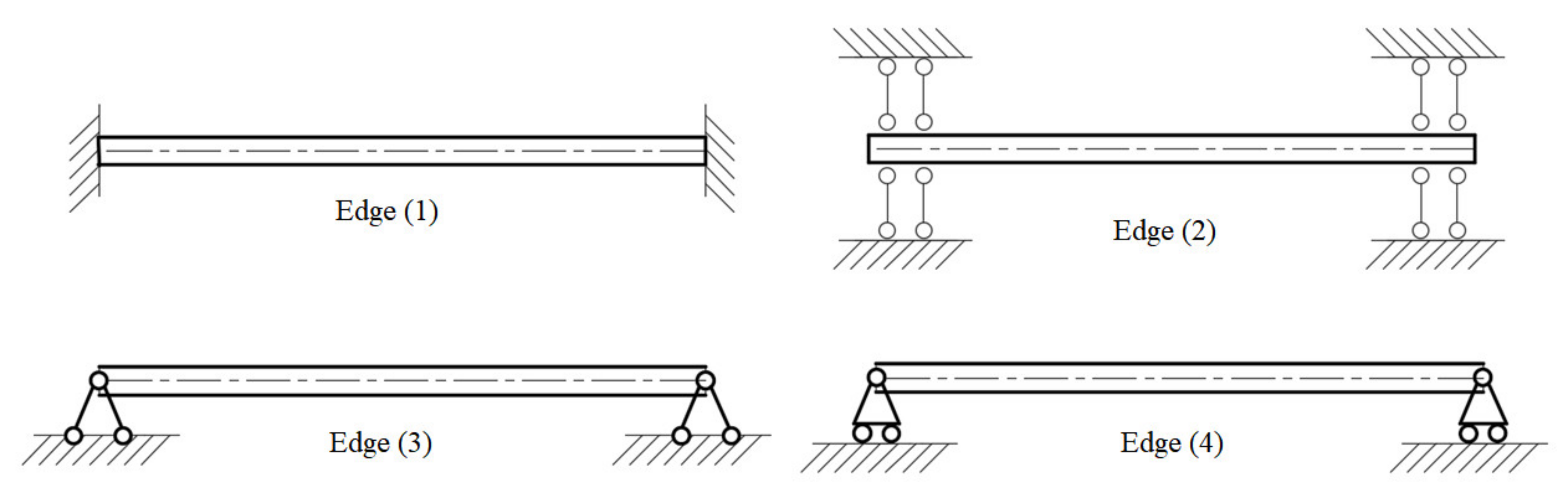
2.3. Boundary Conditions

The following four edge constraints are considered, as shown in Figure 3, that is, for Edge (1), rigidly clamped, we have

$$w=0,\hspace{0.33em}\frac{\mathrm{d}w}{\mathrm{d}r}=0,\hspace{0.33em}u=0\hspace{0.33em}\mathrm{at}\hspace{0.33em}r=a,$$

(35a)

for Edge (2), movably clamped

$$w=0,\hspace{0.33em}\frac{\mathrm{d}w}{\mathrm{d}r}=0,\hspace{0.33em}{N}_r=0\hspace{0.33em}\mathrm{at}\hspace{0.33em}r=a,$$

(35b)

for Edge (3), simply hinged

$$w=0,\hspace{0.33em}{M}_r=0,\hspace{0.33em}u=0\hspace{0.33em}\mathrm{at}\hspace{0.33em}r=a,$$

(35c)

and for Edge (4), simply supported

$$w=0,\hspace{0.33em}{M}_r=0,\hspace{0.33em}{N}_r=0\hspace{0.33em}\mathrm{at}\hspace{0.33em}r=a.$$

(35d)

From Equation (24), the radial displacement, u, of the middle plane can be expressed in terms of the radial force N_r, i.e.,

$$r\frac{\mathrm{d}{N}_r}{\mathrm{d}r}+(1-{\nu }^{+})N_r=0.$$

(36)

For the radial bending moment, M_r, in Equation (19), we introduce 1 + (−dw/dr)² ≈ 1 into the expression of M_r, thus expressing the M_r = 0 only in terms of the deflection w, i.e.,

$$A_2^{+}\left(\frac{{\mathrm{d}}^{2}w}{\mathrm{d}{r}^2}+\frac{{\nu }^{+}}{r}\frac{\mathrm{d}w}{\mathrm{d}r}\right)+A_2^{-}\left(\frac{{\mathrm{d}}^{2}w}{\mathrm{d}{r}^2}+\frac{{\nu }^{-}}{r}\frac{\mathrm{d}w}{\mathrm{d}r}\right)=0.$$

(37)

3. Application of Perturbation Method

3.1. Perturbation Solution

The following dimensionless quantities are introduced

$$P=\frac{q{a}^4}{E_0{t}^4},\hspace{0.33em}\eta =1-\frac{r^2}{a^2},\hspace{0.33em}W=\frac{w}{t},\hspace{0.33em}T=\frac{t}{a},\hspace{0.33em}S=\frac{N_r{a}^2}{E_0{t}^3}$$

(38)

and

$$K=\frac{D^{\ast }}{E_0{t}^3}=\frac{K^{+}+K^{-}}{E_0{t}^3}=\frac{A_2^{+}+A_2^{-}}{E_0{t}^3},\hspace{0.33em}V=\frac{[1-{({\nu }^{+})}^2]A_3}{E_{0}t}.$$

(39)

Thus, Equations (25) and (33) are transformed into

$$\frac{{\mathrm{d}}^2}{\mathrm{d}{\eta }^2}\left[\left(1-\eta \right)S\right]+\frac{V}{2}{\left(\frac{\mathrm{d}W}{\mathrm{d}\eta }\right)}^2=0$$

(40)

and

$$\frac{{\mathrm{d}}^2}{\mathrm{d}{\eta }^2}\left[(1-\eta )\frac{\mathrm{d}W}{\mathrm{d}\eta }-2T^2{(1-\eta )}^2{\left(\frac{\mathrm{d}W}{\mathrm{d}\eta }\right)}^3\right]=-\frac{P}{16K}+\frac{S}{4K}\frac{\mathrm{d}W}{\mathrm{d}\eta }-\frac{T^{2}S}{2K}{\left(\frac{\mathrm{d}W}{\mathrm{d}\eta }\right)}^3.$$

(41)

By means of Equations (22), (37)–(39), the boundary condition Equation (35c) may be transformed into

$$W=0,\hspace{0.33em}{\lambda }_1\frac{{\mathrm{d}}^{2}W}{\mathrm{d}{\eta }^2}-\frac{\mathrm{d}W}{\mathrm{d}\eta }=0,\hspace{0.33em}{\lambda }_2\frac{\mathrm{d}S}{\mathrm{d}\eta }-S=0\hspace{0.33em}\hspace{0.33em}\mathrm{at}\hspace{0.33em}\hspace{0.33em}\eta =0,$$

(42)

where λ₁ and λ₂ are two parameters introduced, and they are [16]

$${\lambda }_1=\frac{2K}{K^{+}(1+{\nu }^{+})+K^{-}(1+{\nu }^{-})},\hspace{0.33em}{\lambda }_2=\hspace{0.33em}\frac{2}{1-{\nu }^{+}}.$$

(43)

It is easy to see that the other three boundary conditions (35a,b,d) may be described as, with λ₁ and λ₂, for rigidly clamped, λ₁ = 0; for movably clamped, λ₁ = λ₂ = 0; and for simply supported, λ₂ = 0. Thus, all that is needed is to solve Equations (40) and (41) under the general conditions (Equation (42)).

In addition, the axisymmetric conditions used for solving gives

$$\frac{\mathrm{d}W}{\mathrm{d}\eta }=0(\ne \hspace{0.33em}\infty )\hspace{0.33em}\mathrm{and}\hspace{0.33em}S\ne \hspace{0.33em}\infty ,\hspace{0.33em}\mathrm{at}\hspace{0.33em}\eta =0.$$

(44)

The dimensionless deflection at the center is chosen as the perturbation parameter [33]

$$W_m={\left(W\right)}_{\eta =1}={\left(\frac{w}{t}\right)}_{r=0}=\frac{w_0}{t},$$

(45)

where w₀ is the central deflection of the circular plate, i.e., the maximum deflection. The dimensionless quantities of P, S, and W are represented by the perturbation parameter

$$P=P\left(W_m\right),\hspace{0.33em}W=W\left(W_m,\eta \right),\hspace{0.33em}S=S\left(W_m,\eta \right).$$

(46)

Thus, P, S, and W are expressed in the form of the power series of W_m

$$\frac{P}{16}=p_1{W}_m+p_2{W}_m^2+p_3{W}_m^3+p_4{W}_m^4+p_5{W}_m^5+\dots ,$$

(47)

$$W={\omega }_1\left(\eta \right)W_m+{\omega }_2\left(\eta \right)W_m^2+{\omega }_3\left(\eta \right)W_m^3+{\omega }_4\left(\eta \right)W_m^4+{\omega }_5\left(\eta \right)W_m^5+\dots ,$$

(48)

$$S=s_1\left(\eta \right)W_m+s_2\left(\eta \right)W_m^2+s_3\left(\eta \right)W_m^3+s_4\left(\eta \right)W_m^4+s_5\left(\eta \right)W_m^5+\dots .$$

(49)

where p_i (i = 1,2,3…) are undetermined constants, and ω_i(η) and s_i(η) (i = 1,2,3…) are undetermined functions with respect to η. The introduction of 1/16 into the expansion of P can make the numerical calculation easier.

• Step 1: p₁, ω₁(η) and s₁(η)

The differential equation used for the solution of s₁(η) can be obtained from the coefficient of W_m in Equation (40)

$$\frac{{\mathrm{d}}^2}{\mathrm{d}{\eta }^2}\left[\left(1-\eta \right)s_1\right]=0,$$

(50)

which should satisfy the boundary conditions as

$$\left\{\begin{array}{l}{\lambda }_2\frac{\mathrm{d}{s}_1}{\mathrm{d}\eta }-s_1=0\hspace{0.33em}\mathrm{at}\hspace{0.33em}\eta =0\\ s_1\ne \infty \hspace{0.33em}\mathrm{at}\hspace{0.33em}\eta =1\end{array}\right..$$

(51)

The solution of Equation (50) under the boundary conditions of Equation (51) is s₁(η) = 0. In the same way, the differential equation used for the solution of ω₁(η) and p₁ can be obtained from the coefficient of W_m in Equation (41)

$$\frac{{\mathrm{d}}^2}{\mathrm{d}{\eta }^2}\left[\left(1-\eta \right)\frac{\mathrm{d}{\omega }_1}{\mathrm{d}\eta }\right]=-\frac{p_1}{K}.$$

(52)

The boundary conditions are

$$\left\{\begin{array}{l}{\omega }_1=0,\hspace{0.33em}{\lambda }_1\frac{{\mathrm{d}}^2{\omega }_1}{\mathrm{d}{\eta }^2}-\frac{\mathrm{d}{\omega }_1}{\mathrm{d}\eta }=0\hspace{0.33em}\mathrm{at}\hspace{0.33em}\eta =0\\ {\omega }_1=1,\hspace{0.33em}\frac{\mathrm{d}{\omega }_1}{\mathrm{d}\eta }\ne \infty \hspace{0.33em}\mathrm{at}\hspace{0.33em}\eta =1\end{array}\right..$$

(53)

Thus, p₁ = 4K/(2λ₁ + 1) and ω₁(η) = (η² + 2λ₁η)/(2λ₁ + 1) may be obtained. It is found that ω₁(η) and p₁ is exactly the solution in the case of small-deflection.

• Step 2: p₂, ω₂(η) and s₂(η)

The differential equation used for the solution of s₂(η) can be obtained from the coefficient of $W_m^2$ in Equation (40), that is

$$\frac{{\mathrm{d}}^2}{\mathrm{d}{\eta }^2}\left[\left(1-\eta \right)s_2\right]+\frac{V}{2}{\left(\frac{\mathrm{d}{\omega }_1}{\mathrm{d}\eta }\right)}^2=0,$$

(54)

which should satisfy the boundary conditions as

$$\left\{\begin{array}{l}{\lambda }_2\frac{\mathrm{d}{s}_2}{\mathrm{d}\eta }-s_2=0\hspace{0.33em}\mathrm{at}\hspace{0.33em}\eta =0\\ s_2\ne \infty \hspace{0.33em}\mathrm{at}\hspace{0.33em}\eta =1\end{array}\right..$$

(55)

Using ω₁(η), obtained in the previous step, the solution of Equation (54) under the boundary conditions of Equation (55) is

$$s_2\left(\eta \right)=\frac{V}{6{\left(1+2{\lambda }_1\right)}^2}\left[{\eta }^3+\left(1+4{\lambda }_1\right){\eta }^2+\left(1+4{\lambda }_1+6{\lambda }_1^2\right)\eta \right.\left.+\left({\lambda }_2+4{\lambda }_1{\lambda }_2+6{\lambda }_1^2{\lambda }_2\right)\right].$$

(56)

The differential equation used for the solutions of ω₂(η) and p₂ from the coefficient of $W_m^2$ is

$$\left\{\begin{array}{l}{\lambda }_2\frac{\mathrm{d}{s}_2}{\mathrm{d}\eta }-s_2=0\hspace{0.33em}\mathrm{at}\hspace{0.33em}\eta =0\\ s_2\ne \infty \hspace{0.33em}\mathrm{at}\hspace{0.33em}\eta =1\end{array}\right..$$

(57)

The boundary conditions are

$$\left\{\begin{array}{l}{\omega }_2=0,\hspace{0.33em}{\lambda }_1\frac{{\mathrm{d}}^2{\omega }_2}{\mathrm{d}{\eta }^2}-\frac{\mathrm{d}{\omega }_2}{\mathrm{d}\eta }=0\hspace{0.33em}\mathrm{at}\hspace{0.33em}\eta =0\\ {\omega }_2=0,\hspace{0.33em}\frac{\mathrm{d}{\omega }_2}{\mathrm{d}\eta }\ne \infty \hspace{0.33em}\mathrm{at}\hspace{0.33em}\eta =1\end{array}\right..$$

(58)

The results ω₂(η) = 0 and p₂ = 0 are easily obtained.

• Step 3: p₃, ω₃(η) and s₃(η)

The differential equation used for the solution of s₃(η) can be obtained from the coefficient of $W_m^3$ in Equation (40), that is

$$\frac{{\mathrm{d}}^2}{\mathrm{d}{\eta }^2}\left[\left(1-\eta \right)s_3\right]+V\frac{\mathrm{d}{\omega }_1}{\mathrm{d}\eta }\frac{\mathrm{d}{\omega }_2}{\mathrm{d}\eta }=0,$$

(59)

which should satisfy the boundary conditions as

$$\left\{\begin{array}{l}{\lambda }_2\frac{\mathrm{d}{s}_3}{\mathrm{d}\eta }-s_3=0\hspace{0.33em}\mathrm{at}\hspace{0.33em}\eta =0\\ s_3\ne \infty \hspace{0.33em}\mathrm{at}\hspace{0.33em}\eta =1\end{array}\right..$$

(60)

The result s₃(η) = 0 is easily obtained. The differential equation used for the solution of ω₃(η) and p₃ from the coefficient of $W_m^3$ is

$$\frac{{\mathrm{d}}^2}{\mathrm{d}{\eta }^2}\left[\left(1-\eta \right)\frac{\mathrm{d}{\omega }_3}{\mathrm{d}\eta }-2T^2{(1-\eta )}^2{\left(\frac{\mathrm{d}{\omega }_1}{\mathrm{d}\eta }\right)}^3\right]=\frac{s_1}{4K}\frac{\mathrm{d}{\omega }_2}{\mathrm{d}\eta }+\frac{s_2}{4K}\frac{\mathrm{d}{\omega }_1}{\mathrm{d}\eta }-\frac{p_3}{K}.$$

(61)

The boundary conditions are

$$\left\{\begin{array}{l}{\omega }_3=0,\hspace{0.33em}{\lambda }_1\frac{{\mathrm{d}}^2{\omega }_3}{\mathrm{d}{\eta }^2}-\frac{\mathrm{d}{\omega }_3}{\mathrm{d}\eta }=0\hspace{0.33em}\mathrm{at}\hspace{0.33em}\eta =0\\ {\omega }_3=0,\hspace{0.33em}\frac{\mathrm{d}{\omega }_3}{\mathrm{d}\eta }\ne \infty \hspace{0.33em}\mathrm{at}\hspace{0.33em}\eta =1\end{array}\right..$$

(62)

Using the ω₁(η) and s₂(η) obtained in the previous steps, the solutions of Equation (61) under the boundary conditions of Equation (62) are

$$p_3=\frac{1}{1080{\left(2{\lambda }_1+1\right)}^4}\left[\begin{array}{l}V\left(\begin{array}{l}1080{\lambda }_1{}^4{\lambda }_2+360{\lambda }_1{}^4+1620{\lambda }_1{}^3{\lambda }_2+840{\lambda }_1{}^3+1080{\lambda }_1{}^2{\lambda }_2\\ +825{\lambda }_1{}^2+350{\lambda }_1{\lambda }_2+388{\lambda }_1+50{\lambda }_2+73\end{array}\right)\\ +K{T}^2\left(69120{\lambda }_1{}^4-172800{\lambda }_1{}^3-34560{\lambda }_1{}^2-17280{\lambda }_1-3456\right)\end{array}\right],$$

(63)

$${\omega }_3\left(\eta \right)=\frac{1}{4320K{\left(2{\lambda }_1+1\right)}^4}\left\{\begin{array}{c}V\left[\begin{array}{c}-\left(4{\lambda }_1+2\right){\eta }^6-\left(36{{\lambda }_1}^2+30{\lambda }_1+6\right){\eta }^5\hfill \\ -\left(150{{\lambda }_1}^3+195{{\lambda }_1}^2+90{\lambda }_1+15\right){\eta }^4\hfill \\ -\left(\begin{array}{c}240{{\lambda }_1}^4+240{{\lambda }_1}^3{\lambda }_2+480{{\lambda }_1}^3+280{{\lambda }_1}^2{\lambda }_2+380{{\lambda }_1}^2\hfill \\ +120{\lambda }_1{\lambda }_2+140{\lambda }_1+20{\lambda }_2+20\hfill \end{array}\right){\eta }^3\hfill \\ +\left(\begin{array}{c}120{{\lambda }_1}^3+120{{\lambda }_1}^2{\lambda }_2+255{{\lambda }_1}^2+80{\lambda }_1{\lambda }_2+178{\lambda }_1\hfill \\ +20{\lambda }_2+43\hfill \end{array}\right){\eta }^2\hfill \\ +\left(\begin{array}{c}240{{\lambda }_1}^4+240{{\lambda }_1}^3{\lambda }_2+510{{\lambda }_1}^3+160{{\lambda }_1}^2{\lambda }_2+356{{\lambda }_1}^2\hfill \\ +40{\lambda }_2{\lambda }_1+86{\lambda }_1\hfill \end{array}\right)\eta \hfill \end{array}\right]\hfill \\ +K{T}^2\left[\begin{array}{c}-\left(27648{\lambda }_1+13824\right){\eta }^5\hfill \\ -\left(103680{{\lambda }_1}^2+17280{\lambda }_1-17280\right){\eta }^4\hfill \\ -\left(138240{{\lambda }_1}^3-69120{{\lambda }_1}^2-69120{\lambda }_1\right){\eta }^3\hfill \\ +\left(69120{{\lambda }_1}^2-17280{\lambda }_1-3456\right){\eta }^2\hfill \\ +\left(138240{{\lambda }_1}^3-34560{{\lambda }_1}^2-6912{\lambda }_1\right)\eta \hfill \end{array}\right]\hfill \end{array}\right\}.$$

(64)

• Step 4: p₃, ω₃(η) and s₃(η)

The differential equation used for the solution of s₄(η) from the coefficient of $W_m^4$ is

$$\frac{{\mathrm{d}}^2}{\mathrm{d}\eta }\left[\left(1-\eta \right)s_4\right]+\frac{V}{2}{\left(\frac{\mathrm{d}{\omega }_2}{\mathrm{d}\eta }\right)}^2+V\frac{\mathrm{d}{\omega }_1}{\mathrm{d}\eta }\frac{\mathrm{d}{\omega }_3}{\mathrm{d}\eta }=0,$$

(65)

which should satisfy the boundary conditions as

$$\left\{\begin{array}{l}{\lambda }_2\frac{\mathrm{d}{s}_4}{\mathrm{d}\eta }-s_4=0\hspace{0.33em}\mathrm{at}\hspace{0.33em}\eta =0\\ s_4\ne \infty \hspace{0.33em}\mathrm{at}\hspace{0.33em}\eta =1\end{array}\right..$$

(66)

Using the ω₁(η) and ω₃(η) obtained in the previous steps, the solution of Equation (65) under the boundary conditions of Equation (66) is

$$s_4\left(\eta \right)=\frac{V}{90720K{\left(2{\lambda }_1+1\right)}^5}\left\{\begin{array}{c}V\left[\begin{array}{c}-\left(18{\lambda }_1+9\right){\eta }^7\hfill \\ -\left(204{{\lambda }_1}^2+180{\lambda }_1+39\right){\eta }^6\hfill \\ -\left(1092{{\lambda }_1}^3+1506{{\lambda }_1}^2+726{\lambda }_1+123\right){\eta }^5\hfill \\ -\left(\begin{array}{c}2772{{\lambda }_1}^4+1512{{\lambda }_1}^3{\lambda }_2+5754{{\lambda }_1}^3+1764{{\lambda }_1}^2{\lambda }_2\hfill \\ +4656{{\lambda }_1}^2+756{\lambda }_1{\lambda }_2+1734{\lambda }_1+126{\lambda }_2+249\hfill \end{array}\right){\eta }^4\hfill \\ -\left(\begin{array}{c}2520{{\lambda }_1}^5+2520{{\lambda }_1}^4{\lambda }_2+7812{{\lambda }_1}^4+4452{{\lambda }_1}^3{\lambda }_2\hfill \\ +8904{{\lambda }_1}^3+2184{{\lambda }_1}^2{\lambda }_2+4341{{\lambda }_1}^2+406{\lambda }_1{\lambda }_2\hfill \\ +698{\lambda }_1-14{\lambda }_2-52\hfill \end{array}\right){\eta }^3\hfill \\ -\left(\begin{array}{c}2520{{\lambda }_1}^5+2520{{\lambda }_1}^4{\lambda }_2+4452{{\lambda }_1}^4+1092{{\lambda }_1}^3{\lambda }_2\hfill \\ +1764{{\lambda }_1}^3-56{{\lambda }_1}^2{\lambda }_2-643{{\lambda }_1}^2-154{\lambda }_1{\lambda }_2\hfill \\ -506{\lambda }_1-14{\lambda }_2-52\hfill \end{array}\right){\eta }^2\hfill \\ +\left(\begin{array}{c}2520{{\lambda }_1}^5+2520{{\lambda }_1}^4{\lambda }_2+6258{{\lambda }_1}^4+2268{{\lambda }_1}^3{\lambda }_2\hfill \\ +5712{{\lambda }_1}^3+896{{\lambda }_1}^2{\lambda }_2+2449{{\lambda }_1}^2+154{\lambda }_1{\lambda }_2\hfill \\ +506{\lambda }_1+14{\lambda }_2+52\hfill \end{array}\right)\eta \hfill \\ +2520{{\lambda }_1}^5{\lambda }_2+2520{{\lambda }_1}^4{{\lambda }_2}^2+6258{{\lambda }_1}^4{\lambda }_2+2268{{\lambda }_1}^3{{\lambda }_2}^2\hfill \\ +5712{{\lambda }_1}^3{\lambda }_2+896{{\lambda }_1}^2{{\lambda }_2}^2+2449{{\lambda }_1}^2{\lambda }_2+154{\lambda }_1{{\lambda }_2}^2\hfill \\ +506{\lambda }_1{\lambda }_2+14{{\lambda }_2}^2+52{\lambda }_2\hfill \end{array}\right]\hfill \\ +K\left[\begin{array}{c}-\left(138240{\lambda }_1+69120\right){\eta }^6\hfill \\ -\left(774144{{\lambda }_1}^2\left.+331776{\lambda }_1-27648\right){\eta }^5\right.\hfill \\ -\left(870912{{\lambda }_1}^3+919296{{\lambda }_1}^2\left.+186624{\lambda }_1-27648\right){\eta }^4\right.\hfill \\ -\left(870912{{\lambda }_1}^3+435456{{\lambda }_1}^2+307584{\lambda }_1-3456\right){\eta }^3\hfill \\ +\left(1064448{{\lambda }_1}^3-919296{{\lambda }_1}^2-404352{\lambda }_1+3456\right){\eta }^2\hfill \\ +\left(\begin{array}{c}2903040{{\lambda }_1}^4+338688{{\lambda }_1}^3-1064448{{\lambda }_1}^2\hfill \\ -404352{\lambda }_1+3456\hfill \end{array}\right)\eta \hfill \\ +2903040{{\lambda }_1}^4{\lambda }_2+338688{{\lambda }_1}^3{\lambda }_2-1064448{{\lambda }_1}^2{\lambda }_2\hfill \\ -404352{\lambda }_1{\lambda }_2+3456{\lambda }_2\hfill \end{array}\right]\hfill \end{array}\right\}.$$

(67)

The differential equation used for the solutions of ω₄(η) and p₄ from the coefficient of $W_m^4$ is

$$\begin{array}{l}\frac{{\mathrm{d}}^2}{\mathrm{d}\eta }\left[\left(1-\eta \right)\frac{\mathrm{d}{\omega }_3}{\mathrm{d}\eta }-6T^2{(1-\eta )}^2{\left(\frac{\mathrm{d}{\omega }_1}{\mathrm{d}\eta }\right)}^2\frac{\mathrm{d}{\omega }_2}{\mathrm{d}\eta }\right]\\ =\frac{s_1}{4K}\frac{\mathrm{d}{\omega }_3}{\mathrm{d}\eta }+\frac{s_2}{4K}\frac{\mathrm{d}{\omega }_2}{\mathrm{d}\eta }+\frac{s_3}{4K}\frac{\mathrm{d}{\omega }_1}{\mathrm{d}\eta }-\frac{T^2{s}_1}{2K}{\left(\frac{\mathrm{d}{\omega }_1}{\mathrm{d}\eta }\right)}^3-\frac{p_4}{K}.\end{array}$$

(68)

The boundary conditions are

$$\left\{\begin{array}{l}{\omega }_4=0,\hspace{0.33em}{\lambda }_1\frac{{\mathrm{d}}^2{\omega }_4}{\mathrm{d}{\eta }^2}-\frac{\mathrm{d}{\omega }_4}{\mathrm{d}\eta }=0\hspace{0.33em}\mathrm{at}\hspace{0.33em}\eta =0\\ {\omega }_4=0,\hspace{0.33em}\frac{\mathrm{d}{\omega }_4}{\mathrm{d}\eta }\ne \infty \hspace{0.33em}\mathrm{at}\hspace{0.33em}\eta =1\end{array}\right..$$

(69)

The results ω₄(η) = 0 and p₄ = 0 are easily obtained.

Thus, the unknown constants p₁ and p₃ and functions ω₁(η), ω₃(η), s₂(η), and s₄(η) have been determined. The remaining solutions of p_i, ω_i(η), and s_i(η) (i = 5,6,7…) can be obtained through similar calculations. The further calculations will not be described in detail.

Lastly, we obtain the perturbation solution of S, P, and W with respect to W_m

$$\begin{array}{c}S=\frac{V{W}_m^2}{6{\left(2{\lambda }_1+1\right)}^2}\left[{\eta }^3+\left(1+4{\lambda }_1\right){\eta }^2+\left(1+4{\lambda }_1+6{\lambda }_1^2\right)\eta +{\lambda }_2+4{\lambda }_1{\lambda }_2+6{\lambda }_1^2{\lambda }_2\right]\hfill \\ +\frac{V{W}_m^4}{90720K{\left(2{\lambda }_1+1\right)}^5}\left\{\begin{array}{c}V\left[\begin{array}{c}-\left(18{\lambda }_1+9\right){\eta }^7-\left(204{{\lambda }_1}^2+180{\lambda }_1+39\right){\eta }^6\hfill \\ -\left(1092{{\lambda }_1}^3+1506{{\lambda }_1}^2\right.\left.+726{\lambda }_1+123\right){\eta }^5\hfill \\ -\left(\begin{array}{c}2772{{\lambda }_1}^4+1512{{\lambda }_1}^3{\lambda }_2+5754{{\lambda }_1}^3+1764{{\lambda }_1}^2{\lambda }_2\hfill \\ +4656{{\lambda }_1}^2+756{\lambda }_1{\lambda }_2+1734{\lambda }_1+126{\lambda }_2+249\hfill \end{array}\right){\eta }^4\hfill \\ -\left(\begin{array}{c}2520{{\lambda }_1}^5+2520{{\lambda }_1}^4{\lambda }_2+7812{{\lambda }_1}^4+4452{{\lambda }_1}^3{\lambda }_2+8904{{\lambda }_1}^3\hfill \\ +2184{{\lambda }_1}^2{\lambda }_2+4341{{\lambda }_1}^2+406{\lambda }_1{\lambda }_2+698{\lambda }_1-14{\lambda }_2-52\hfill \end{array}\right){\eta }^3\hfill \\ -\left(\begin{array}{c}2520{{\lambda }_1}^5+2520{{\lambda }_1}^4{\lambda }_2+4452{{\lambda }_1}^4+1092{{\lambda }_1}^3{\lambda }_2+1764{{\lambda }_1}^3\hfill \\ -56{{\lambda }_1}^2{\lambda }_2-643{{\lambda }_1}^2-154{\lambda }_1{\lambda }_2-506{\lambda }_1-14{\lambda }_2-52\hfill \end{array}\right){\eta }^2\hfill \\ +\left(\begin{array}{c}2520{{\lambda }_1}^5+2520{{\lambda }_1}^4{\lambda }_2+6258{{\lambda }_1}^4+2268{{\lambda }_1}^3{\lambda }_2+5712{{\lambda }_1}^3\hfill \\ +896{{\lambda }_1}^2{\lambda }_2+2449{{\lambda }_1}^2+154{\lambda }_1{\lambda }_2+506{\lambda }_1+14{\lambda }_2+52\hfill \end{array}\right)\eta \hfill \\ +2520{{\lambda }_1}^5{\lambda }_2+2520{{\lambda }_1}^4{{\lambda }_2}^2+6258{{\lambda }_1}^4{\lambda }_2+2268{{\lambda }_1}^3{{\lambda }_2}^2+5712{{\lambda }_1}^3{\lambda }_2\hfill \\ +896{{\lambda }_1}^2{{\lambda }_2}^2+2449{{\lambda }_1}^2{\lambda }_2+154{\lambda }_1{{\lambda }_2}^2+506{\lambda }_1{\lambda }_2+14{{\lambda }_2}^2+52{\lambda }_2\hfill \end{array}\right]\hfill \\ +K{T}^2\left[\begin{array}{c}-\left(138240{\lambda }_1+69120\right){\eta }^6\hfill \\ -\left(774144{{\lambda }_1}^2\right.\left.+331776{\lambda }_1-27648\right){\eta }^5\hfill \\ -\left(870912{{\lambda }_1}^3+919296{{\lambda }_1}^2+186624{\lambda }_1-27648\right){\eta }^4\hfill \\ -\left(870912{{\lambda }_1}^3+435456{{\lambda }_1}^2+307584{\lambda }_1-3456\right){\eta }^3\hfill \\ +\left(1064448{{\lambda }_1}^3-919296{{\lambda }_1}^2-404352{\lambda }_1+3456\right){\eta }^2\hfill \\ +\left(\begin{array}{c}2903040{{\lambda }_1}^4+338688{{\lambda }_1}^3-1064448{{\lambda }_1}^2\hfill \\ -404352{\lambda }_1+3456\hfill \end{array}\right)\eta \hfill \\ +2903040{{\lambda }_1}^4{\lambda }_2+338688{{\lambda }_1}^3{\lambda }_2-1064448{{\lambda }_1}^2{\lambda }_2\hfill \\ -404352{\lambda }_1{\lambda }_2+3456{\lambda }_2\hfill \end{array}\right]\hfill \end{array}\right\}\hfill \end{array},$$

(70)

$$\begin{array}{l}\frac{P}{16}=\frac{4K{W}_m}{2{\lambda }_1+1}\\ +\frac{W_m^3}{1080{\left(2{\lambda }_1+1\right)}^4}\left[\begin{array}{l}V\left(\begin{array}{l}1080{\lambda }_1{}^4{\lambda }_2+360{\lambda }_1{}^4+1620{\lambda }_1{}^3{\lambda }_2+840{\lambda }_1{}^3+1080{\lambda }_1{}^2{\lambda }_2\\ +825{\lambda }_1{}^2+350{\lambda }_1{\lambda }_2+388{\lambda }_1+50{\lambda }_2+73\end{array}\right)\\ +K{T}^2\left(69120{\lambda }_1{}^4-172800{\lambda }_1{}^3-34560{\lambda }_1{}^2-17280{\lambda }_1-3456\right)\end{array}\right]\end{array},$$

(71)

$$\begin{array}{c}W=\frac{W_m}{2{\lambda }_1+1}\left({\eta }^2+2{\lambda }_1\eta \right)\hfill \\ +\frac{W_m^3}{4320K{\left(2{\lambda }_1+1\right)}^4}\left\{\begin{array}{c}V\left[\begin{array}{c}-\left(4{\lambda }_1+2\right){\eta }^6\hfill \\ -\left(36{{\lambda }_1}^2+30{\lambda }_1+6\right){\eta }^5\hfill \\ -\left(150{{\lambda }_1}^3+195{{\lambda }_1}^2\right.\left.+90{\lambda }_1+15\right){\eta }^4\hfill \\ -\left(\begin{array}{c}240{{\lambda }_1}^4+240{{\lambda }_1}^3{\lambda }_2+480{{\lambda }_1}^3+280{{\lambda }_1}^2{\lambda }_2+380{{\lambda }_1}^2\hfill \\ +120{\lambda }_1{\lambda }_2+140{\lambda }_1+20{\lambda }_2+20\hfill \end{array}\right){\eta }^3\hfill \\ +\left(120{{\lambda }_1}^3+120{{\lambda }_1}^2{\lambda }_2+255{{\lambda }_1}^2+80{\lambda }_1{\lambda }_2+178{\lambda }_1+20{\lambda }_2+43\right){\eta }^2\hfill \\ +\left(\begin{array}{c}240{{\lambda }_1}^4+240{{\lambda }_1}^3{\lambda }_2+510{{\lambda }_1}^3+160{{\lambda }_1}^2{\lambda }_2\hfill \\ +356{{\lambda }_1}^2+40{\lambda }_2{\lambda }_1+86{\lambda }_1\hfill \end{array}\right)\eta \hfill \end{array}\right]\hfill \\ +K{T}^2\left[\begin{array}{c}-\left(27648{\lambda }_1+13824\right){\eta }^5\hfill \\ -\left(103680{{\lambda }_1}^2+17280{\lambda }_1-17280\right){\eta }^4\hfill \\ -\left(138240{{\lambda }_1}^3-69120{{\lambda }_1}^2-69120{\lambda }_1\right){\eta }^3\hfill \\ +\left(69120{{\lambda }_1}^2-17280{\lambda }_1-3456\right){\eta }^2\hfill \\ +\left(138240{{\lambda }_1}^3-34560{{\lambda }_1}^2-6912{\lambda }_1\right)\eta \hfill \end{array}\right]\hfill \end{array}\right\}\hfill \end{array}.$$

(72)

3.2. Stress Analysis

For the purpose of studying the stress of each point on the plate, it is necessary to derive the stretching stress from membrane force and the bending stress from bending moment. Let ${{\sum }^{\prime }}_r\left(\eta \right)$ be the dimensionless stretching stress at the middle plane of the plate ${{\sigma }^{\prime }}_r$, and let ${{\sum }^{″}}_r\left(\eta \right)$ be the dimensionless bending stress on the convex surface ${\sigma }^{″}$, i.e.,

$${{\sum }^{\prime }}_r\left(\eta \right)=\frac{{{\sigma }^{\prime }}_r{a}^2}{E_0{t}^2}$$

(73)

$${{\sum }^{″}}_r\left(\eta \right)=\frac{{{\sigma }^{″}}_r{a}^2}{E_0{t}^2}.$$

(74)

Allowing ${{\sum }^{\prime }}_r\left(\eta \right)\approx s_2(\eta )W_m^2+s_4(\eta )W_m^4$, the dimensionless stretching stress at the edge of the plate is

$$\begin{array}{c}{{\sum }^{\prime }}_r\left(0\right)=\frac{V{W}_m^2}{6{\left(2{\lambda }_1+1\right)}^2}\left({\lambda }_2+4{\lambda }_1{\lambda }_2+6{\lambda }_1^2{\lambda }_2\right)\hfill \\ +\frac{V{W}_m^4}{90720K{\left(2{\lambda }_1+1\right)}^5}\left[\begin{array}{c}V\left(\begin{array}{c}2520{{\lambda }_1}^5{\lambda }_2+2520{{\lambda }_1}^4{{\lambda }_2}^2+6258{{\lambda }_1}^4{\lambda }_2+2268{{\lambda }_1}^3{{\lambda }_2}^2+5712{{\lambda }_1}^3{\lambda }_2\hfill \\ +896{{\lambda }_1}^2{{\lambda }_2}^2+2449{{\lambda }_1}^2{\lambda }_2+154{\lambda }_1{{\lambda }_2}^2+506{\lambda }_1{\lambda }_2+14{{\lambda }_2}^2+52{\lambda }_2\hfill \end{array}\right)\hfill \\ +K{T}^2\left(\begin{array}{c}2903040{{\lambda }_1}^4{\lambda }_2+338688{{\lambda }_1}^3{\lambda }_2-1064448{{\lambda }_1}^2{\lambda }_2\hfill \\ -404352{\lambda }_1{\lambda }_2+3456{\lambda }_2\hfill \end{array}\right)\hfill \end{array}\right]\hfill \end{array}$$

(75)

and the stretching stress at the center of the plate is

$$\begin{array}{c}{{\sum }^{\prime }}_r\left(1\right)=\frac{V{W}_m^2}{6{\left(2{\lambda }_1+1\right)}^2}\left(3+8{\lambda }_1+6{\lambda }_1^2+{\lambda }_2+4{\lambda }_1{\lambda }_2+6{\lambda }_1^2{\lambda }_2\right)\hfill \\ +\frac{V{W}_m^4}{90720K{\left(2{\lambda }_1+1\right)}^5}\left[\begin{array}{c}V\left(\begin{array}{c}2520{{\lambda }_1}^5{\lambda }_2-2520{{\lambda }_1}^5+2520{{\lambda }_1}^4{{\lambda }_2}^2+3738{{\lambda }_1}^4{\lambda }_2-8778{{\lambda }_1}^4\hfill \\ +2268{{\lambda }_1}^3{{\lambda }_2}^2+924{{\lambda }_1}^3{\lambda }_2-11802{{\lambda }_1}^3+896{{\lambda }_1}^2{{\lambda }_2}^2-547{{\lambda }_1}^2{\lambda }_2\hfill \\ -7615{{\lambda }_1}^2+154{\lambda }_1{{\lambda }_2}^2-348{\lambda }_1{\lambda }_2-2344{\lambda }_1+14{{\lambda }_2}^2-32{\lambda }_2-264\hfill \end{array}\right)\hfill \\ +K{T}^2\left(\begin{array}{c}2903040{{\lambda }_1}^4{\lambda }_2+2903040{{\lambda }_1}^4+338688{{\lambda }_1}^3{\lambda }_2-338688{{\lambda }_1}^3\hfill \\ -1064448{{\lambda }_1}^2{\lambda }_2-4112640{{\lambda }_1}^2-404352{\lambda }_1{\lambda }_2-1772928{\lambda }_1\hfill \\ +3456{\lambda }_2-3456\hfill \end{array}\right)\hfill \end{array}\right]\hfill \end{array}.$$

(76)

The dimensionless bending stress on the convex surface is

$${{\sigma }^{″}}_r=\frac{12M_r{t}_1}{t^3},$$

(77)

where t₁ is the height of tensile section in the plate and, for convenience in the next computation, we define its dimensionless form as T₁ = t₁/t; at the same time, T₂ = t₂/t. Substituting Equations (19) and (77) into Equation (74) gives

$${{\sum }^{″}}_r\left(\eta \right)\approx \frac{24\left[K^{+}\left(1+{\nu }^{+}\right)+K^{-}\left(1+{\nu }^{-}\right)\right]T_1}{T}\frac{\mathrm{d}W}{\mathrm{d}\eta }-\frac{48K(1-\eta )T_1}{T}\frac{{\mathrm{d}}^{2}W}{\mathrm{d}{\eta }^2}.$$

(78)

Substituting the expressions of $W(\eta )\approx {\omega }_1\left(\eta \right)W_m+{\omega }_3\left(\eta \right)W_m^3$ into Equation (78), the dimensionless bending stress at the edge of the plate is obtained, i.e.,

$$\begin{array}{c}{{\sum }^{\prime \prime }}_r\left(0\right)=\frac{T_1{W}_m}{2{\lambda }_1+1}\left\{96K-48\left[K^{+}\left(1+{\nu }^{+}\right)+K^{-}\left(1+{\nu }^{-}\right)\right]{\lambda }_1\right\}\hfill \\ -\frac{T_1{W}_m^3}{1080{\left(2{\lambda }_1+1\right)}^4}\left\{\begin{array}{c}12\left[K^{+}\left(1+{\nu }^{+}\right)+K^{-}\left(1+{\nu }^{-}\right)\right]\left[\begin{array}{c}V\left(\begin{array}{c}120{{\lambda }_1}^4+120{{\lambda }_1}^3{\lambda }_2\hfill \\ +255{{\lambda }_1}^3+80{{\lambda }_1}^2{\lambda }_2\hfill \\ +178{{\lambda }_1}^2+20{\lambda }_1{\lambda }_2\hfill \\ +43{\lambda }_1\hfill \end{array}\right)\hfill \\ +K{T}^2\left(\begin{array}{c}69120{{\lambda }_1}^3-17280{{\lambda }_1}^2\hfill \\ -3456{\lambda }_1\hfill \end{array}\right)\hfill \end{array}\right]\hfill \\ +V\left(\begin{array}{c}120{{\lambda }_1}^3+120{{\lambda }_1}^2{\lambda }_2+255{{\lambda }_1}^2\hfill \\ +80{\lambda }_1{\lambda }_2+178{\lambda }_1+20{\lambda }_2+43\hfill \end{array}\right)+K{T}^2\left(\begin{array}{c}69120{{\lambda }_1}^2-17280{\lambda }_1\hfill \\ -3456\hfill \end{array}\right)\hfill \end{array}\right\}\hfill \end{array},$$

(79)

and the dimensionless bending stress at the center of the plate is

$$\begin{array}{c}{{\sum }^{\prime \prime }}_r\left(1\right)=\frac{T_1{W}_m}{2{\lambda }_1+1}\left\{48({\lambda }_1+1)\left[K^{+}\left(1+{\nu }^{+}\right)+K^{-}\left(1+{\nu }^{-}\right)\right]\right\}\hfill \\ -\frac{T_1{W}_m^3}{1080K{\left(2{\lambda }_1+1\right)}^4}\left\{12\left[K^{+}\left(1+{\nu }^{+}\right)+K^{-}\left(1+{\nu }^{-}\right)\right]\left[\begin{array}{c}V\left(\begin{array}{c}240{{\lambda }_1}^4+240{{\lambda }_1}^3{\lambda }_2+645{{\lambda }_1}^3\hfill \\ +220{{\lambda }_1}^2{\lambda }_2+347{{\lambda }_1}^2\hfill \\ +80{\lambda }_1{\lambda }_2+256{\lambda }_1+10{\lambda }_2+38\hfill \end{array}\right)\hfill \\ +K{T}^2\left(\begin{array}{c}138240{{\lambda }_1}^3+51840{{\lambda }_1}^2\hfill \\ +20736{\lambda }_1+3456\hfill \end{array}\right)\hfill \end{array}\right]\right\}\hfill \end{array}.$$

(80)

Via the above stress expressions, we may analyze the yield problem of the bimodular FGM plate in large deformation. Let three principal stresses be σ₁, σ₂, and σ₃. The yield condition gives

$${\left({\sigma }_1-{\sigma }_2\right)}^2+{\left({\sigma }_2-{\sigma }_3\right)}^2+{\left({\sigma }_3-{\sigma }_1\right)}^2=2{\sigma }_y^2,$$

(81)

where σ_y is the yield stress.

At the edge of the plate, due to u = r(N_θ − ν⁺N_r)/A₃ = 0, it is found that

$${\sigma }_1={\sigma }_{re},\hspace{1em}{\sigma }_2={\sigma }_{te}={\nu }^{+}{\sigma }_{re},\hspace{1em}{\sigma }_3<<{\sigma }_{re},$$

(82)

where σ_re and σ_te are the radial and circumferential stresses on the convex surface of the plate edge, respectively. Supposing σ₃ = 0, we can obtain

$${\sigma }_{re}=\frac{{\sigma }_y}{\sqrt{1-{\nu }^{+}+{({\nu }^{+})}^2}},\hspace{0.33em}{\sigma }_{te}=\frac{{\nu }^{+}{\sigma }_y}{\sqrt{1-{\nu }^{+}+{({\nu }^{+})}^2}}.$$

(83)

Therefore, the dimensionless yield stress calculated with the radial stress is

$$\frac{{\sigma }_y{a}^2}{E_0{t}^2}=\sqrt{1-{\nu }^{+}+{({\nu }^{+})}^2}\left({\sum }_r^{\prime }(0)+{\sum }_r^{″}(0)\right).$$

(84)

Substituting Equations (75) and (79) into Equation (84), the dimensionless yield stress at the edge is

$$\begin{array}{c}\frac{{\sigma }_y{a}^2}{E_0{t}^2}=\hfill \\ \left\{\begin{array}{c}\frac{T_1{W}_m\sqrt{1-{\nu }^{+}+{\left({\nu }^{+}\right)}^2}}{2{\lambda }_1+1}\left\{96K-48\left[K^{+}\left(1+{\nu }^{+}\right)+K^{-}\left(1+{\nu }^{-}\right)\right]{\lambda }_1\right\}\hfill \\ +\frac{V{W}_m^2\sqrt{1-{\nu }^{+}+{\left({\nu }^{+}\right)}^2}}{6{\left(2{\lambda }_1+1\right)}^2}\left({\lambda }_2+4{\lambda }_1{\lambda }_2+6{\lambda }_1^2{\lambda }_2\right)\hfill \\ -\frac{T_1{W}_m^3\sqrt{1-{\nu }^{+}+{\left({\nu }^{+}\right)}^2}}{1080{\left(2{\lambda }_1+1\right)}^4}\left\{\begin{array}{c}12\left[K^{+}\left(1+{\nu }^{+}\right)+K^{-}\left(1+{\nu }^{-}\right)\right]\left[\begin{array}{c}V\left(\begin{array}{c}120{{\lambda }_1}^4+120{{\lambda }_1}^3{\lambda }_2\hfill \\ +255{{\lambda }_1}^3+80{{\lambda }_1}^2{\lambda }_2\hfill \\ +178{{\lambda }_1}^2+20{\lambda }_1{\lambda }_2\hfill \\ +43{\lambda }_1\hfill \end{array}\right)\hfill \\ +K{T}^2\left(\begin{array}{c}69120{{\lambda }_1}^3\hfill \\ -17280{{\lambda }_1}^2\hfill \\ -3456{\lambda }_1\hfill \end{array}\right)\hfill \end{array}\right]\hfill \\ +V\left(\begin{array}{c}120{{\lambda }_1}^3+120{{\lambda }_1}^2{\lambda }_2\hfill \\ +255{{\lambda }_1}^2+80{\lambda }_1{\lambda }_2\hfill \\ +178{\lambda }_1+20{\lambda }_2+43\hfill \end{array}\right)+K{T}^2\left(\begin{array}{c}69120{{\lambda }_1}^2\hfill \\ -17280{\lambda }_1\hfill \\ -3456\hfill \end{array}\right)\hfill \end{array}\right\}\hfill \\ +\frac{V{W}_m^4\sqrt{1-{\nu }^{+}+{\left({\nu }^{+}\right)}^2}}{90720K{\left(2{\lambda }_1+1\right)}^5}\left[\begin{array}{c}V\left(\begin{array}{c}2520{{\lambda }_1}^5{\lambda }_2+2520{{\lambda }_1}^4{{\lambda }_2}^2+6258{{\lambda }_1}^4{\lambda }_2+2268{{\lambda }_1}^3{{\lambda }_2}^2\hfill \\ +5712{{\lambda }_1}^3{\lambda }_2+896{{\lambda }_1}^2{{\lambda }_2}^2+2449{{\lambda }_1}^2{\lambda }_2+154{\lambda }_1{{\lambda }_2}^2\hfill \\ +506{\lambda }_1{\lambda }_2+14{{\lambda }_2}^2+52{\lambda }_2\hfill \end{array}\right)\hfill \\ +K{T}^2\left(\begin{array}{c}2903040{{\lambda }_1}^4{\lambda }_2+338688{{\lambda }_1}^3{\lambda }_2-1064448{{\lambda }_1}^2{\lambda }_2\hfill \\ -404352{\lambda }_1{\lambda }_2+3456{\lambda }_2\hfill \end{array}\right)\hfill \end{array}\right]\hfill \end{array}\right\}\hfill \end{array}.$$

(85)

Next, we will derive the yield stress at the center of the plate. The principal stresses should be equal at the center, i.e.,

$${\sigma }_1={\sigma }_2={\sigma }_{rc},\hspace{1em}{\sigma }_3<<{\sigma }_{rc},$$

(86)

where σ_re is the radial stress on the convex surface of the plate center. Similarly, letting σ₃ = 0, we have

$${\sigma }_{rc}={\sigma }_y.$$

(87)

The dimensionless yield stress calculated with the radial stress is

$$\frac{{\sigma }_y{a}^2}{E_0{t}^2}={\sum }_r^{\prime }(1)+{\sum }_r^{″}(1).$$

(88)

Substituting Equations (76) and (80) into Equation (88), the dimensionless yield stress at the center is

$$\begin{array}{c}\frac{{\sigma }_y{a}^2}{E_0{t}^2}=\frac{T_1{W}_m}{2{\lambda }_1+1}\left\{48({\lambda }_1+1)\left[K^{+}\left(1+{\nu }^{+}\right)+K^{-}\left(1+{\nu }^{-}\right)\right]\right\}\hfill \\ +\frac{V{W}_m^2}{6{\left(2{\lambda }_1+1\right)}^2}\left(3+8{\lambda }_1+6{\lambda }_1^2+{\lambda }_2+4{\lambda }_1{\lambda }_2+6{\lambda }_1^2{\lambda }_2\right)\hfill \\ -\frac{T_1{W}_m^3}{1080K{\left(2{\lambda }_1+1\right)}^4}\left\{12\left[K^{+}\left(1+{\nu }^{+}\right)+K^{-}\left(1+{\nu }^{-}\right)\right]\left[\begin{array}{c}V\left(\begin{array}{c}240{{\lambda }_1}^4+240{{\lambda }_1}^3{\lambda }_2+645{{\lambda }_1}^3\hfill \\ +220{{\lambda }_1}^2{\lambda }_2+347{{\lambda }_1}^2+80{\lambda }_1{\lambda }_2\hfill \\ +256{\lambda }_1+10{\lambda }_2+38\hfill \end{array}\right)\hfill \\ +K{T}^2\left(\begin{array}{c}138240{{\lambda }_1}^3+20736{\lambda }_1\hfill \\ +51840{{\lambda }_1}^2+3456\hfill \end{array}\right)\hfill \end{array}\right]\right\}\hfill \\ +\frac{V{W}_m^4}{90720K{\left(2{\lambda }_1+1\right)}^5}\left[\begin{array}{c}V\left(\begin{array}{c}2520{{\lambda }_1}^5{\lambda }_2-2520{{\lambda }_1}^5+2520{{\lambda }_1}^4{{\lambda }_2}^2+3738{{\lambda }_1}^4{\lambda }_2-8778{{\lambda }_1}^4\hfill \\ +2268{{\lambda }_1}^3{{\lambda }_2}^2+924{{\lambda }_1}^3{\lambda }_2-11802{{\lambda }_1}^3+896{{\lambda }_1}^2{{\lambda }_2}^2-547{{\lambda }_1}^2{\lambda }_2\hfill \\ -7615{{\lambda }_1}^2+154{\lambda }_1{{\lambda }_2}^2-348{\lambda }_1{\lambda }_2-2344{\lambda }_1+14{{\lambda }_2}^2-32{\lambda }_2-264\hfill \end{array}\right)\hfill \\ +K{T}^2\left(\begin{array}{c}2903040{{\lambda }_1}^4{\lambda }_2+2903040{{\lambda }_1}^4+338688{{\lambda }_1}^3{\lambda }_2-338688{{\lambda }_1}^3\hfill \\ -1064448{{\lambda }_1}^2{\lambda }_2-4112640{{\lambda }_1}^2-404352{\lambda }_1{\lambda }_2-1772928{\lambda }_1\hfill \\ +3456{\lambda }_2-3456\hfill \end{array}\right)\hfill \end{array}\right]\hfill \end{array}.$$

(89)

In addition, under the Edges (1), (2), and (4), the dimensionless yield stresses at the center and at the peripheral edge of the plate can be easily obtained by letting λ₁ and λ₂ equal the corresponding values.

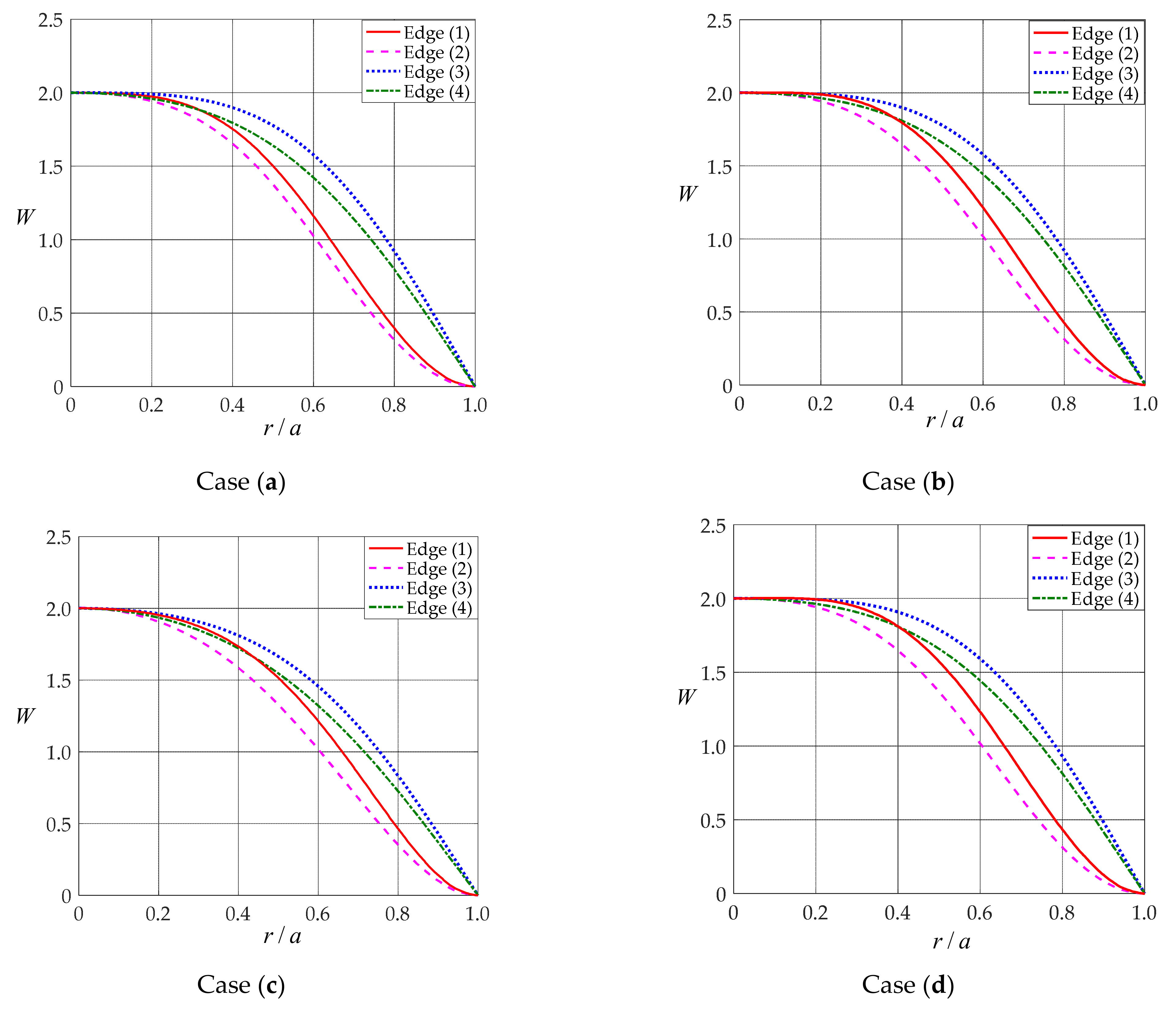
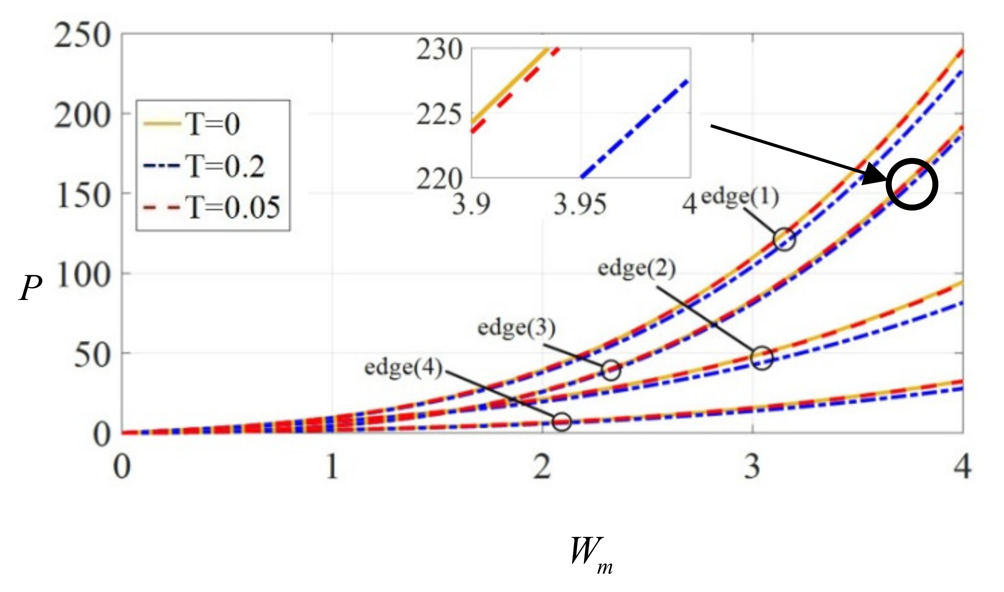
4. Results and Discussions

The regression of the perturbation solutions of S, P, and W obtained in Section 3.1 need to be discussed. Comparing Equations (70)–(72) in this paper with Equations (104)–(106) in [31], it is found that, if T = 0 in Equations (70)–(72), the perturbation solutions of S, P, and W will be the same as those presented in [31], which verifies, to some extent, the reliability of the perturbation solutions obtained in this paper.

4.1. Determination of the Neutral Layer

The position of the unknown neutral layer should first be determined. Letting the integral of the items of z in Equation (18) be equal to zero, i.e., $A_1^{+}+A_1^{-}=0$, one has

$$\begin{array}{l}{A}_1^{+}+A_1^{-}\\ =\frac{1}{1-{({\nu }^{+})}^2}\left[\frac{E_0{t}^2}{{\alpha }_1^2}+\left(\frac{t_{1}t}{{\alpha }_1}-\frac{t^2}{{\alpha }_1^2}\right)E_0{e}^{{\alpha }_1{t}_1/t}\right]+\frac{1}{1-{({\nu }^{-})}^2}\left[-\frac{E_0{t}^2}{{\alpha }_2^2}+\left(\frac{t_{2}t}{{\alpha }_2}+\frac{t^2}{{\alpha }_2^2}\right)E_0{e}^{-{\alpha }_2{t}_2/t}\right]=0.\end{array}$$

(90)

Multiplying Equation (90) by ${\alpha }_1^2$${\alpha }_2^2$[1−(ν⁺)²][1−(ν⁻)²]/(E₀t²), it is found that

$${\alpha }_2^2[1-{({\nu }^{-})}^2]\left[1+\left({\alpha }_1{T}_1-1\right)e^{{\alpha }_1{T}_1}\right]+{\alpha }_1^2[1-{({\nu }^{+})}^2]\left[-1+\left({\alpha }_2{T}_2+1\right)e^{-{\alpha }_2{T}_2}\right]=0.$$

(91)

Expanding $e^{{\alpha }_1{T}_1}$ and $e^{-{\alpha }_2{T}_2}$ in Equation (91) into Taylor series of T₁ and T₂, respectively, i.e., letting

$$\left\{\begin{array}{l}{e}^{{\alpha }_1{T}_1}=1+{\alpha }_1{T}_1+\frac{1}{2}{\alpha }_1^2{T}_1^2+\dots +\frac{1}{n!}{({\alpha }_1{T}_1)}^n+\dots \\ e^{-{\alpha }_2{T}_2}=1-{\alpha }_2{T}_2+\frac{1}{2}{\alpha }_2^2{T}_2^2+\dots +\frac{1}{n!}{(-{\alpha }_2{T}_2)}^n+\dots \end{array}\right.$$

(92)

and substituting the first two terms into Equation (91) yields

$$[1-{({\nu }^{-})}^2]T_1^2-[1-{({\nu }^{+})}^2]T_2^2=0.$$

(93)

Additionally combining T₁ + T₂ = 1, the expressions of the tensile and compressive heights are, respectively

$$T_1=\frac{t_1}{t}=\frac{-1+{({\nu }^{+})}^2\pm \sqrt{[1-{({\nu }^{+})}^2][1-{({\nu }^{-})}^2]}}{{({\nu }^{+})}^2-{({\nu }^{-})}^2}$$

(94)

$$T_2=\frac{t_2}{t}=\frac{1-{({\nu }^{-})}^2\pm \sqrt{[1-{({\nu }^{+})}^2][1-{({\nu }^{-})}^2]}}{{({\nu }^{+})}^2-{({\nu }^{-})}^2}.$$

(95)

It should be noted here that, from the above equation, it seems that the tensile and compressive heights depend only on the Poisson ratio and are independent of the modulus of elasticity. In fact, both two physical quantities participate in the determination of the heights, in which the influences caused by E⁺(z) and E⁻(z) is embodied by α₁ and α₂, which existed in the original Equation (84). However, after taking the first two items of the expansion T₁ and T₂, the influences of the modulus of elasticity happens to disappear, which is the reason why Equations (94) and (95) contains only the Poisson ratio. If we take more items from Equation (92), a more complicated expression containing α₁ and α₂ will be obtained, and the solution in this case cannot be explicitly expressed.

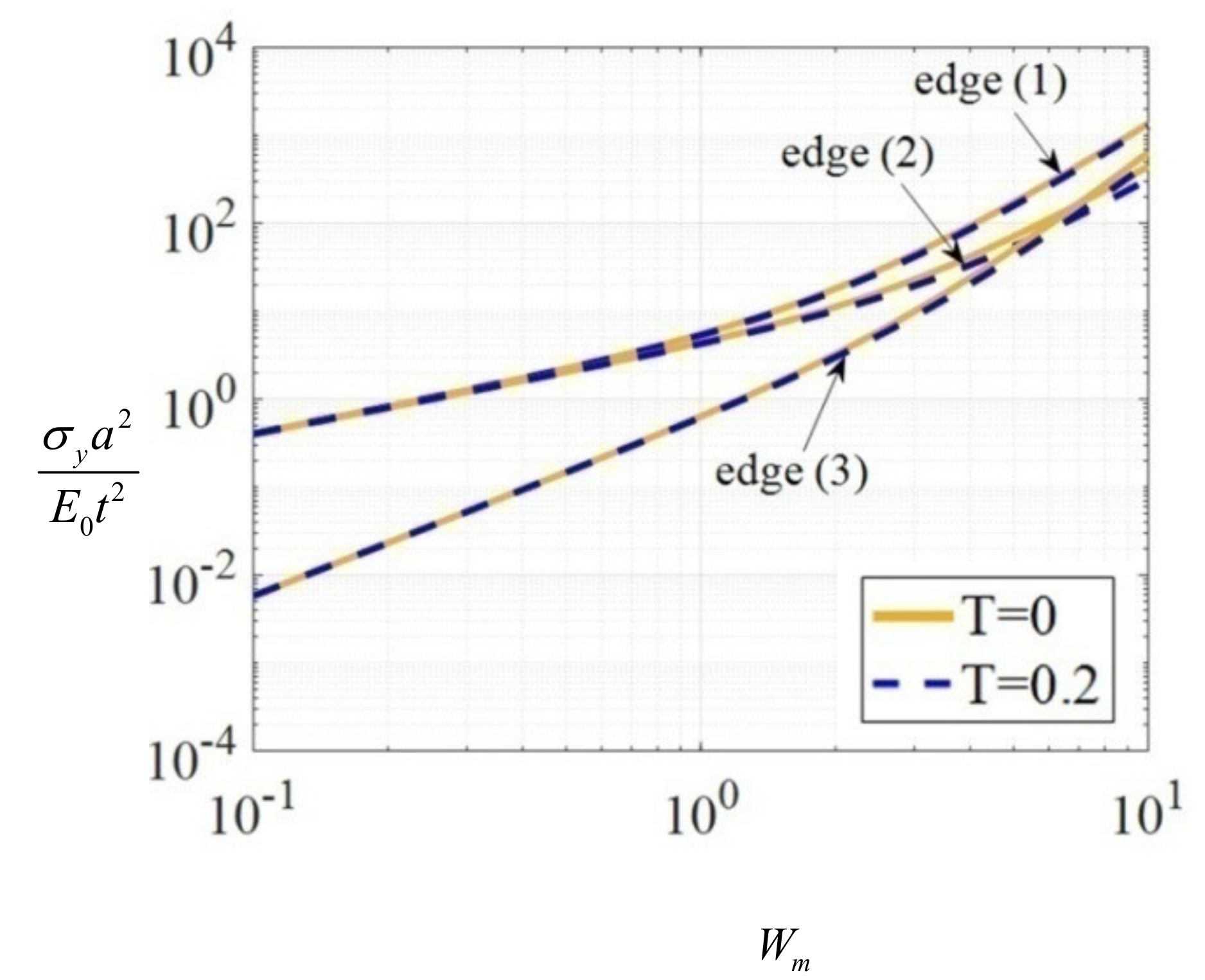
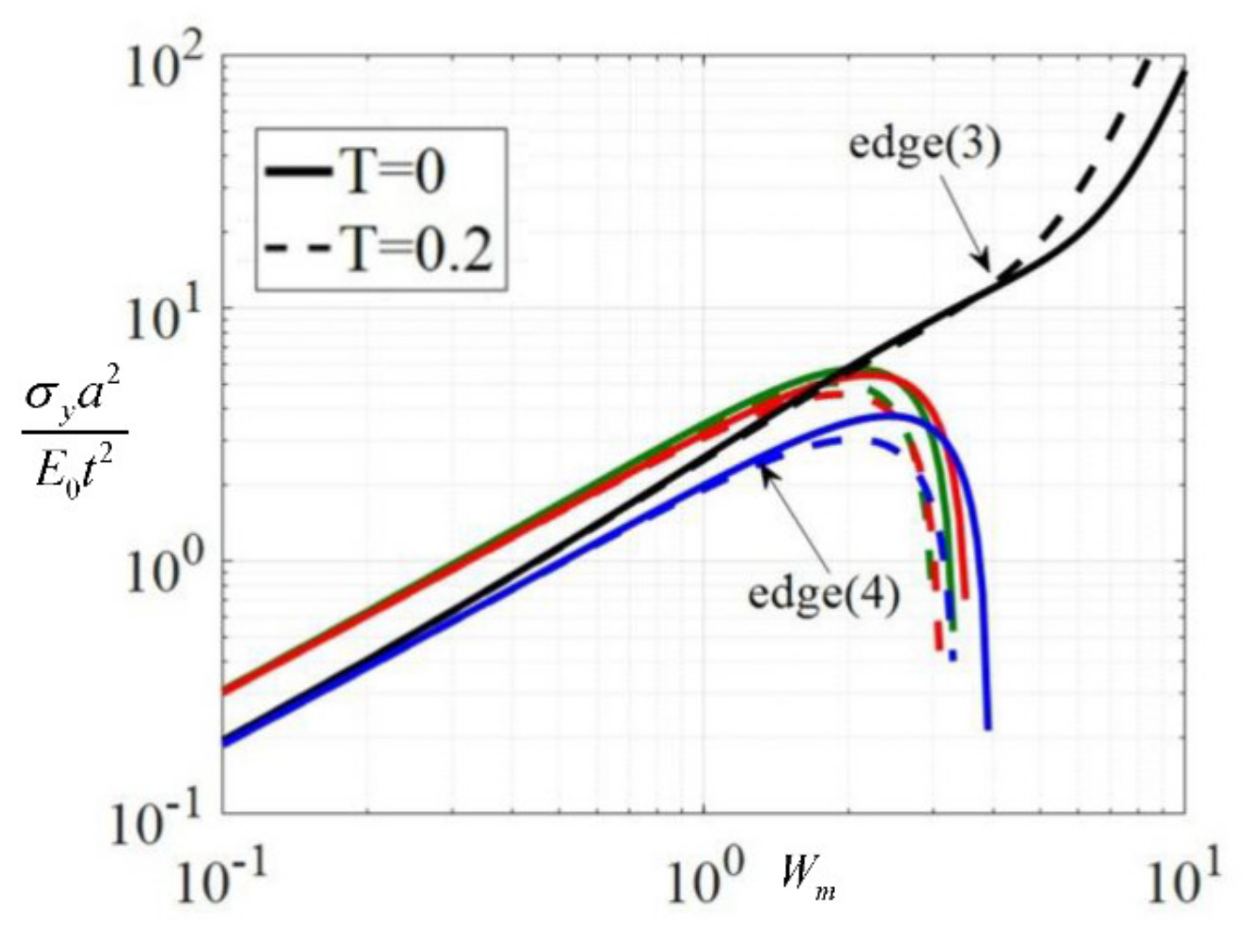
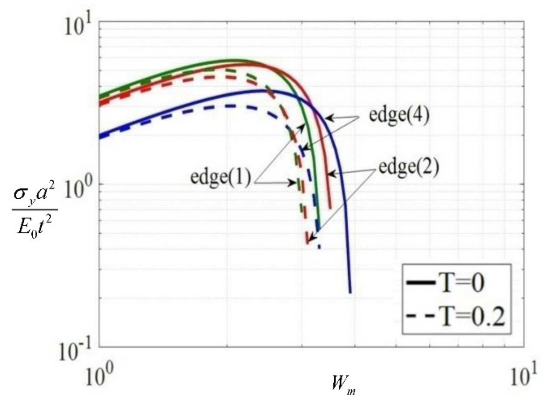
4.2. Effect of Small-Rotation-Angle Assumption on Loads vs. Central Deflection

There are four cases of the positive or negative signs of graded parameters α₁ and α₂ in Equation (1): case (a) α₁ > 0, α₂ > 0; case (b) α₁ < 0, α₂ < 0; case (c) α₁ > 0, α₂ < 0; and case (d) α₁ < 0, α₂ > 0. If the positive or negative signs of α₁ and α₂ are determined, the relative magnitude among the modulus of the neutral layer, E₀, the tensile modulus, E⁺(z), and compressive modulus, E⁻(z), will be accordingly defined, i.e., for case (a), we have E⁺(z) > E₀ > E⁻(z); for case (b), E⁺(z) < E₀ < E⁻(z); for case (c), E⁺(z) > E₀, E⁻(z) > E₀; and for case (d), E⁺(z) < E₀, E⁻(z) < E₀.

Some numerical examples were carried out to discuss the effect of the small-rotation-angle assumption on the response of the bimodular FGM plate. The FGM we are familiar with may be manufactured using powder metallurgy techniques from a mixture of ceramic and metal. Generally, metals exhibit good tensile properties and can be considered as materials in the tensile zone, whereas ceramics exhibit good compressive properties and can be considered as materials in the compressive zone. The Poisson ratios of the tensile and compressive zones is taken as ν⁺ = 0.35 (manganese bronze) and ν⁻= 0.25 (silica ceramic), respectively. Moreover, in order to be able to describe the four cases of the relative magnitude among E⁺(z), E₀, and E⁻(z), we chose four groups of data: case (a), α₁ = 0.5, α₂ = 0.1; case (b), α₁ = −0.5, α₂ = −0.1; case (c), α₁ = 0.5, α₂ = −0.1; and case (d), α₁ = −0.5, α₂ = 0.1. From Equations (94) and (95), the dimensionless heights of the tensile and compressive zones are T₁ = 0.4821 and T₂ = 0.5179, respectively. Thus, using Equations (18), (39), and (43) and also based on the known ν⁺, ν⁻, α₁, α₂, T₁, and T₂, the values of λ₁, λ₂, K, and V may be determined, and they are listed in

Table 1. Values of K, V, λ₁, and λ₂ under Edges (1)–(4) and cases (a)–(d).

Conditions	Case (a)	Case (b)	Case (c)	Case (d)
Edge (1)	K = 0.0986,V = 1.0015, λ1 = 0,λ2 = 3.0769.	K = 0.0869,V = 1.0195, λ1 = 0,λ2 = 3.0769.	K = 0.1024,V = 1.0015, λ1 = 0,λ2 = 3.0769.	K = 0.0831,V = 1.0195, λ1 = 0,λ2 = 3.0769.
Edge (2)	K = 0.0986,V = 1.0015, λ1 = λ2 = 0.	K = 0.0869,V = 1.0195, λ1 = λ2 = 0.	K = 0.1024,V = 1.0015, λ1 = λ2 = 0.	K = 0.0831,V = 1.0195, λ1 = λ2 = 0.
Edge (3)	K = 0.0986,V = 1.0015, λ1 = 1.5363,λ2 = 3.0769.	K = 0.0869,V = 1.0195, λ1 = 1.5493,λ2 = 3.0769.	K = 0.1024,V = 1.0015, λ1 = 1.5386,λ2 = 3.0769.	K = 0.0831,V = 1.0195, λ1 = 1.5470,λ2 = 3.0769.
Edge (4)	K = 0.0986,V = 1.0015, λ1 = 1.5363,λ2 = 0.	K = 0.0869,V = 1.0195, λ1 = 1.5493,λ2 = 0.	K = 0.1024,V = 1.0015, λ1 = 1.5386,λ2 = 0.	K = 0.0831,V = 1.0195, λ1 = 1.5470,λ2 = 0.

. At the same time, by substituting λ₁, λ₂, K, and V into Equations (71) and (72), the expressions of P and W with respect to W_m are obtained, and they are listed in

Table 2. P and W with respect to W_m.

Cases	Formulas
	(1) Rigidly clamped
(a)	P = (3.3656 − 5.0466T2)Wm3 + 6.3082 Wm W = [−0.0047η6 − (0.0141 + 3.2T2)η5 − (0.0353 − 4T2)η4 − 0.1918η3 + (0.2459 − 0.8T2)η2]Wm3 + η2Wm
(b)	P = (3.4263 − 4.4498T2)Wm3 + 5.5623Wm W = [−0.0054η6 − (0.0163 + 3.2T2)η5 − (0.0407 − 4T2)η4 − 0.2214η3 + (0.2839 − 0.8T2)η2]Wm3 + η2Wm
(c)	P = (3.3656 − 5.2430T2)Wm3 + 6.5538Wm W = [−0.0045η6 − (0.0136 + 3.2T2)η5 − (0.0339 − 4T2)η4 − 0.1846η3 + (0.2367 − 0.8T2)η2]Wm3 + η2Wm
(d)	P = (3.4263 − 4.2534T2)Wm3 + 5.3167Wm W = [−0.0057η6 − (0.0170 + 3.2T2)η5 − (0.0426 − 4T2)η4 − 0.2316η3 + (0.2970 − 0.8T2)η2]Wm3 + η2Wm
	(2) Movably clamped
(a)	P = (1.0831 − 5.0466T2)Wm3 + 6.3082Wm W = [−0.0047η6 − (0.0141 + 3.2T2)η5 − (0.0353 − 4T2)η4 − 0.0470η3 + (0.1011 − 0.8T2)η2]Wm3 + η2Wm
(b)	P = (1.1026 − 4.4498T2)Wm3 + 5.5623Wm W = [−0.0054η6 − (0.0163 + 3.2T2)η5 − (0.0407 − 4T2)η4 − 0.054η3 + (0.1168 − 0.8T2)η2]Wm3 + η2Wm
(c)	P = (1.0831 − 5.2430T2)Wm3 + 6.5538Wm W = [−0.0045η6 − (0.0136 + 3.2T2)η5 − (0.0339 − 4T2)η4 − 0.0453η3 + (0.0973 − 0.8T2)η2]Wm3 + η2Wm
(d)	P = (1.1026 − 4.2534T2)Wm3 + 5.3167Wm W = [−0.0057η6 − (0.0170 + 3.2T2)η5 − (0.0426 − 4T2)η4 − 0.0568η3 + (0.1222 − 0.8T2)η2]Wm3 + η2Wm
	(3) Simply hinged
(a)	P = (2.9072 − 1.8742T2)Wm3 + 1.5489Wm W = [−0.000069η6 − (0.001172 + 0.047371T2)η5 − (0.009895 + 0.213703T2)η4 − (0.081639 + 0.195165T2)η3 + (0.022780 + 0.112025T2)η2 + (0.069996 + 0.344215T2)η]Wm3 + (0.245540η2 + 0.754460η)Wm
(b)	P = (2.9617 − 1.6315T2)Wm3 + 1.3571Wm W = [−0.000079η6 − (0.001337 + 0.046479T2)η5 − (0.011358 + 0.211935T2)η4 − (0.093963 + 0.197765T2)η3 + (0.026042 + 0.111302T2)η2 + (0.080693 + 0.344876T2)η]Wm3 + (0.243988η2 + 0.756011η)Wm
(c)	P = (2.9072 − 1.9428T2)Wm3 + 1.6074Wm W = [ − 0.000067η6 − (0.001125 + 0.047212T2)η5 − (0.009514 + 0.213389T2)η4 − (0.078537 + 0.195631T2)η3 + (0.021888 + 0.111897T2)η2 + (0.067355 + 0.344334T2)η]Wm3 + (0.245263η2 + 0.754737η)Wm
(d)	P = (2.9614 − 1.5630T2)Wm3 + 1.2987Wm W = [−0.000083η6 − (0.001401 + 0.046633T2)η5 − (0.011895 + 0.212243T2)η4 − (0.098356 + 0.197315T2)η3 + (0.027292 + 0.111429T2)η2 + (0.084443 + 0.344763T2)η]Wm3 + (0.244258η2 + 0.755741η)Wm
	(4) Simply supported
(a)	P = (0.4135 − 1.8742T2)Wm3 + 1.5489Wm W = [−0.000069η6 − (0.001172 + 0.047371T2)η5 − (0.009895 + 0.213703T2)η4 − (0.035988 + 0.195165T2)η3 + (0.011571 + 0.112025T2)η2 + (0.035553 + 0.344215T2)η]Wm3 + (0.245540η2 + 0.754460η)Wm
(b)	P = (0.4203 − 1.6315T2)Wm3 + 1.3571Wm W = [−0.000079η6 − (0.001337 + 0.046479T2)η5 − (0.011358 + 0.211935T2)η4 − (0.041540 + 0.197765T2)η3 + (0.013252 + 0.111302T2)η2 + (0.041061 + 0.344876T2)η]Wm3 + (0.243988η2 + 0.756011η)Wm
(c)	P = (0.4135 − 1.9428T2)Wm3 + 1.6074Wm W = [−0.000067η6 − (0.001125 + 0.047212T2)η5 − (0.009514 + 0.213389T2)η4 − (0.034638 + 0.195631T2)η3 + (0.011121 + 0.111897T2)η2 + (0.034223 + 0.344334T2)η]Wm3 + (0.245263η2 + 0.754737η)Wm
(d)	P = (0.4204 − 1.5630T2)Wm3 + 1.2987Wm W = [−0.000083η6 − (0.001401 + 0.046633T2)η5 − (0.011895 + 0.212243T2)η4 − (0.043460 + 0.197315T2)η3 + (0.013883 + 0.111429T2)η2 + (0.042956 + 0.344763T2)η]Wm3 + (0.244258η2+0.755741η)Wm

.

Generally speaking, the bending stiffness of the plate depends partly on the magnitude of the modulus of elasticity of the materials; the bigger the modulus of elasticity, the stronger the bending-resistant capacity. Obviously, among the four cases of the tensile modulus, compressive modulus, and the neutral layer modulus, case (c) has the strongest bending-resistant capacity because there exists the relations E⁺(z) > E₀ and E⁻(z) > E₀. On the contrary, case (d) has the weakest capacity resisting deformation due to E⁺(z) < E₀ and E⁻(z) < E₀. In addition, the deformation of the thin plate is greatly affected by the boundary constraint. Next, a numerical example is given to illustrate the effect of the four boundary constraints on the deformation of thin plates. The deflection curves of the bimodular FGM thin plate under four edge constraint conditions when the central deflection of the thin plate, W_m, reaches 2, are then plotted, as shown in Figure 4, where Case (a) represents E⁺(z) > E₀ > E⁻(z); Case (b) represents E⁺(z) < E₀ < E⁻(z); Case (c) represents E⁺(z) > E₀, E⁻(z) > E₀; and Case (d) represents E⁺(z) < E₀, E⁻(z) < E₀. Note that a coordinate transform is carried out, i.e., the coordinate variable (𝜂 = 1 − 𝑟²/𝑎²) in the deflection expressions in Table 2 should be transformed into the ratio of the radial coordinate to the radius of the thin plate (r/a) to show the deflection curves.

By comparing the four deflection diagrams in Figure 4, it can be seen that the two graded indices in the tensile and compressive zones, α₁ and α₂, do not change the real shape of the deflection curves of the thin plate. In the Cases a, b, c, and d, the rotation angle of the deflection curve of Edge (2) at r/a = 0 is the largest among the four constraint conditions, while the rotation angle of the deflection curve of Edge (3) at r/a = 0 is the smallest. Moreover, for the same central deflection, when 0 < r/a < 1, the deformation degree of the thin plate under the constraint of the Edge (2) is the smallest, and the deformation of the thin plate under the constraint of the Edge (3) is the largest. In addition, when 0 < r/a < 0.4, the deflection curves of Edge (1) and Edge (4) are relatively close in all four Cases (a, b, c, d).

In the following content, we will focus our discussion on just one case, i.e., Case (a) E⁺(z) > E₀ > E⁻(z), which corresponds to the parameters α₁ = 0.5, α₂ = 0.1, and consider the bimodular FGM circular plate with the different dimensionless thicknesses, T = 0, 0.05 and 0.2, respectively, where T = 0 represents the perturbation solution from [31] with the small-rotation-angle assumption. Figure 5 shows the variations of the dimensionless external loads, P, with central deflection W_m under the constraints of Edges (1)–(4). The concrete values of external loads and the errors between the conditions T ≠ 0 and T = 0 (i.e., the errors caused by the small-rotation-angle assumption) are listed in

Table 3. Computational values of P and errors for T ≠ 0 and T = 0.

Edges	Wm	T = 0	T = 0.05		T = 0.2
			Present	Errors 1	Present	Errors
(1)	1	9.6738	9.6612	0.13%	9.4719	2.13%
	2	39.5411	39.4401	0.26%	37.9262	4.26%
	3	109.7953	109.4547	0.31%	104.3450	5.22%
	4	240.6300	239.8225	0.34%	227.7106	5.67%
(2)	1	7.3913	7.3786	0.17%	7.1894	2.81%
	2	21.2809	21.1800	0.48%	19.6660	8.21%
	3	48.1673	47.8266	0.71%	42.7170	12.76%
	4	94.5486	93.7411	0.86%	81.6292	15.83%
(3)	1	4.4561	4.4514	0.11%	4.3811	1.71%
	2	26.3552	26.3177	0.14%	25.7554	2.33%
	3	83.1403	83.0137	0.15%	81.1161	2.50%
	4	192.2544	191.9545	0.16%	187.4563	2.56%
(4)	1	1.9624	1.9577	0.24%	1.8875	3.97%
	2	6.4060	6.3685	0.59%	5.8062	10.33%
	3	15.8118	15.6850	0.81%	13.7876	14.68%
	4	32.6609	32.3610	0.93%	27.8628	17.22%

¹ Subtract the values at T = 0 from the values at T ≠ 0 and then divide by the values at T = 0.

, in which the dimensionless central deflection take different values, i.e., W_m = 1, 2, 3, 4.

From Figure 5, it is easy to see that, under any of the four boundary constraints, for the curves of external loads vs. central deflection, the curve T = 0.05 is very close to the curve T = 0; however, there is an obvious distance between curve T = 0.2 and curve T = 0, especially under the Edge (1) and Edge (2) constraints. Moreover, for the same central deflection, the external load acting on the thin plate is always the smallest under the Edge (4) constraint, and it is always the largest under the Edge (1) constraint. Besides, from Table 3, it may be readily seen that, for the same magnitude value of the central deflection, the external loads calculated by the perturbation solutions presented here (for T ≠ 0) are uniformly smaller than those calculated by the perturbation solutions presented in [31] (for T = 0). For example, under the Edge (4) constraint, when W_m = 4, the external load calculated by the solution presented in [31] is 32.6609 (T = 0), while the external loads calculated by the solution presented here are 32.3610 for T = 0.05 and 27.8628 for T = 0.2. In this case, the relative error between the external load for T = 0 and that for T = 0.05 is only 0.93%, which is less than the allowable error of 1% for precision instruments. The relative error between the present solution and the existing solution is very small, which can, to some extent, be taken as a criterion to judge the reliability of the perturbation solutions presented here. Furthermore, under the Edge (4) constraint, when W_m = 4 and T = 0.2, the relative error between the present solution and the existing solution has reached 17.22%, which is caused by the small-rotation-angle assumption and is even greater than the allowable error in engineering (<15%). In other words, in this case, the error of external load calculated by the perturbation solution with the small-rotation-angle assumption in [31] is 17.22%; accordingly, the computational accuracy of the external load without the small-rotation-angle assumption in this paper is improved by 17.22% in comparison with the external load for [31].

On the other hand, no matter how small rotation angle β is, because sinβ ≠ tanβ, adopting the small-rotation-angle assumption (assuming that sinβ ≈ tanβ) will always create the obtained perturbation solution with a certain error. It can also be found from Table 3 that, as the central deflection, W_m, increases, the relative error between the external loads calculated by the perturbation solution in this paper and in [31] also increases. With the increase of the central deflection, W_m, the rotation angle, β, will also increase; therefore, the error brought by the small-rotation-angle assumption will also increase accordingly.

At the same time, we also find that, for different boundary constraints, the effects of the small-rotation-angle assumption on the response of plates are different. From Table 3, it can be seen that, for the same central deflection, the errors of external load under the Edges (1) and (3) constraints are less than those under the Edge (2) and (4) constraints; for example, when W_m = 3 and T = 0.2, the errors of Edges (1), (3), (2), and (4) are 5.22%, 2.50%, 12.76%, and 14.68%, respectively. Because the small-rotation-angle assumption is abandoned in this paper, the established governing equation exists with five terms related to the rotation angle that are not available in the classic Föppl–von Kármán equation. Besides, when the perturbation method is adopted to solve the governing equations, the external load is expanded to the power series of the perturbation parameter (i.e., W_m). It can be considered that the computational accuracy of the perturbation solution is not only related to the perturbation parameter, but also to the rotation angle at the location of the expansion point. From the four cases in Figure 4, it can be seen that, at the center part of the plate, the rotation angles of the thin plate under the Edge (1) and (3) constraints are smaller than those under the Edge (2) and (4) constraints; thus, the computational accuracies of the perturbation solutions of the Edge (1) and (3) constraints are higher than those of Edges (2) and (4). Therefore, it is necessary to abandon the small-rotation-angle assumption in the large deformation problem of bimodular FGM thin circular plates when the central deflection or the dimensionless thickness is large, especially for Edge (2), movably clamped, and Edge (4), simply supported.

4.3. Effect of Small-Rotation-Angle Assumption on Yield Stress

Next, under a logarithmic coordinates system, we plot the curves of yield stress at the edge of the plate under three edges constraints when T = 0 and T = 0.2, as shown in Figure 6. Note that σ_y = 0 at the edge of the plate under Edge (4), simply supported, constraint. The concrete values of the yield stress at the edge of the plate under Edges (1), (2), and (3) and the errors between the conditions T ≠ 0 and T = 0 (i.e., the errors induced by the small-rotation-angle assumption) are listed in

Table 4. Computational values of edge yield stress under Edges (1), (2), and (3).

Wm	Edge (1)			Edge (2)			Edge (3)
	T = 0	T = 0.2	Errors 1	T = 0	T = 0.2	Errors	T = 0	T = 0.2	Errors
0.1	0.4065	0.4063	0.03%	0.4014	0.4012	0.03%	0.005819	0.005823	0.07%
0.5	2.2427	2.2269	0.70%	2.0555	2.0395	0.78%	0.1477	0.1486	0.61%
1.0	5.4757	5.3515	2.27%	4.4151	4.2868	2.91%	0.6230	0.6382	2.44%
1.5	10.5032	10.0911	3.92%	7.3830	6.9500	5.87%	1.5233	1.6003	5.05%
2.0	18.1728	17.2124	5.29%	11.2633	10.2368	9.11%	3.0104	3.2538	8.09%
2.5	29.3752	27.5316	6.28%	16.3600	14.3552	12.25%	5.3111	5.9052	11.19%
3.0	45.0445	41.9145	6.95%	22.9774	19.5131	15.08%	8.7169	9.9489	14.13%
4.0	93.7361	86.5809	7.63%	41.9906	33.7789	19.56%	20.3338	24.2275	19.15%
5.0	172.5850	159.1258	7.80%	70.7358	54.6973	22.67%	42.4889	50.9949	20.02%
6.0	290.6206	268.2546	7.70%	111.6461	83.9315	24.82%	79.8466	96.5583	20.93%
7.0	457.5646	423.4637	7.45%	167.1544	123.1447	26.33%	139.1077	168.626	21.22%
8.0	683.8308	635.0410	7.13%	239.6937	174.0000	27.41%	225.0096	276.3082	22.80%
9.0	980.5251	914.0653	6.78%	331.6971	238.1605	28.20%	349.3262	430.1164	23.13%
10.0	1359.4454	1272.4067	6.40%	445.5976	317.2895	28.79%	510.8678	641.9639	25.66%

¹ Subtract the values at T = 0.2 from the values at T = 0 and then divide by the values at T = 0.

. We also plot the curves of yield stress at the center of the plate under the four edge constraints under a logarithmic coordinates system, as shown in Figure 7, and the local magnification of center yield stresses is clearly shown in Figure 8, in which the center deflection is equal to 1 to 10.

It is easy to see from Figure 6 that the yield stress at the edge of the plate increases with the increase of the central deflection W_m. When 0.1 < W_m < 1, the yield stress at the edge of the plate under the Edge (3) constraint is much smaller than that under the Edge (1) and (2) constraints. The difference of yield stress curves at the edge of the plate between T = 0 and T = 0.2 under the logarithmic coordinate systems is not obvious in Figure 6. From Table 4, it can be seen that the errors caused by the small-rotation-angle assumption under the Edge (1) and (3) constraints are less than 8%, but under the Edge (2) constraint, the errors caused by the small-rotation-angle assumption are quite large, and the maximum error has reached 28.8% (The allowable error for civil engineering is within 15%). For the Edge (2) constraint, substituting λ₁ = λ₂ = 0 into Equation (85), there is only one item related to the parameter T, which is an important parameter that affects the computational accuracy of the perturbation solution, but for the Edge (1) and (3) constraints, after substituting their corresponding λ₁ and λ₂ into Equation (85), the positive and negative signs of the terms related to parameter T are opposite and may be offset during the calculation. Therefore, the yield stress at the edge of the plate under the Edge (2) constraint has a huge difference between T = 0 and T ≠ 0. This indicates that the effect of the small-rotation-angle assumption on the yield stress at the edge of the plate under the Edge (2) constraint is far greater than those under the Edge (1) and (3) constraints.

From Figure 7 and Figure 8, it can be easily seen that, for the maximum deflection with the same magnitude, the yield stresses at the center of plate under the Edge (1), (2), and (4) constraints of T = 0.2 are obviously smaller than those of T = 0. Moreover, for the same central deflection, the yield stresses at the center of the plate under the Edge (1) and (2) constraints are greater than those under the Edge (3) and (4) constraints. Comparing Figure 7 with Figure 6, it can be seen that the effect of the small-rotation-angle assumption on the yield stress at the center is greater than that on the yield stress at the edge. The above numerical examples are sufficient to prove that the computational accuracy of the perturbation solution abandoning the small-rotation-angle assumption is improved.

5. Conclusions

In this study, the large deformation problem of a bimodular FGM thin circular plate subjected to a transversely uniformly-distributed load is investigated, under the condition of giving up the small-rotation-angle assumption. The effects of the small-rotation-angle assumption on the responses of the bimodular FGM thin circular plate are discussed using specific numerical examples. The following three conclusions can be drawn:

(i) The improved governing equations for the large deformation problem of the bimodular functionally-graded thin circular plate without small-rotation-angle assumption can be regressed to the classical Föppl–von Kármán equations, and the corresponding perturbation solutions can also be regressed to the perturbation solutions with small-rotation-angle assumption. This verifies, to some extent, the reliability of the perturbation solutions obtained in this paper.

(ii) The perturbation solutions presented in this paper have higher computational accuracy in comparison with the existing perturbation solutions. For example, in the numerical examples carried out in Section 4, the computational accuracies of external load and yield stress are improved by 17.22% and 28.79% at most, respectively. For the maximum deflection with the same magnitude, the external load calculated by the perturbation solution presented in this paper would be less than the external load from the previous solution, and the errors of the perturbation solutions caused by the small-rotation-angle assumption under the movably clamped and simply supported constraints are larger than those under the rigidly clamped and the simply hinged constraints.

(iii) The small-rotation-angle assumption has little influence on the yield stress at the edge of plate, while it has great influence on the yield stress at the center of the plate, especially for the constraint cases with edges rigidly clamped, movably clamped, and simply supported.

The problem and method presented in this study can be used for further research work. In particular, the problem concerning small-rotation-angle assumption may be extended into the establishment of mathematical models with buckling and contact phenomena for elastic plates [42], because the buckling problem of an elastic plate is usually accompanied by its large deformation. In addition, the single-parameter perturbation method based on the central deflection in this study may also be extended to the so-called multi-parameters perturbation method [43] that has been successfully used for investigating functionally-graded, thin, circular piezoelectric plates. The relative work is in progress.

References

1. Barak, M.M.; Currey, J.D.; Weiner, S.; Shahar, R. Are tensile and compressive Young’s moduli of compact bone different. J. Mech. Behav. Biomed. Mater. 2009, 2, 51–60. [Google Scholar] [CrossRef] [PubMed]
2. Destrade, M.; Gilchrist, M.D.; Motherway, J.A.; Murphy, J.G. Bimodular rubber buckles early in bending. Mech. Mater. 2010, 42, 469–476. [Google Scholar] [CrossRef] [Green Version]
3. Jones, R.M. Apparent flexural modulus and strength of multimodulus materials. J. Compos. Mater. 1976, 10, 342–354. [Google Scholar] [CrossRef]
4. Jones, R.M. Stress-strain relations for materials with different moduli in tension and compression. AIAA J. 1977, 15, 16–23. [Google Scholar] [CrossRef]
5. Bert, C.W. Models for fibrous composites with different properties in tension and compression. J. Eng. Mater. Technol. 1977, 99, 344–349. [Google Scholar] [CrossRef]
6. Bruno, D.; Lato, S.; Sacco, E. Nonlinear analysis of bimodular composite plates under compression. Comput. Mech. 1994, 14, 28–37. [Google Scholar] [CrossRef]
7. Tseng, Y.P.; Lee, C.T. Bending analysis of bimodular laminates using higher-order finite strip method. Compos. Struct. 1995, 30, 341–350. [Google Scholar] [CrossRef]
8. Zinno, R.; Greco, F. Damage evolution in bimodular laminated composite under cyclic loading. Compos. Struct. 2001, 53, 381–402. [Google Scholar] [CrossRef]
9. Ganapathi, M.; Patel, B.P.; Lele, A.V. Static analysis of bimodulus laminated composite plates subjected to mechanical loads using higher-order shear deformation theory. J. Reinf. Plast. Compos. 2004, 23, 1159–1171. [Google Scholar] [CrossRef]
10. Khan, A.H.; Patel, B.P. Nonlinear periodic response of bimodular laminated composite annular sector plates. Compos. Part B Eng. 2019, 169, 96–108. [Google Scholar] [CrossRef]
11. Ambartsumyan, S.A. Elasticity Theory of Different Modulus; Wu, R.F.; Zhang, Y.Z., Translators; China Railway Publishing House: Beijing, China, 1986. [Google Scholar]
12. Yao, W.J.; Ye, Z.M. Analytical solution for bending beam subject to lateral force with different modulus. Appl. Math. Mech. Engl. Ed. 2004, 25, 1107–1117. [Google Scholar]
13. He, X.T.; Chen, S.L.; Sun, J.Y. Applying the equivalent section method to solve beam subjected lateral force and bending-compression column with different moduli. Int. J. Mech. Sci. 2007, 49, 919–924. [Google Scholar] [CrossRef]
14. Zhao, H.L.; Ye, Z.M. Analytic elasticity solution of bi-modulus beams under combined loads. Appl. Math. Mech. Engl. Ed. 2015, 36, 427–438. [Google Scholar] [CrossRef]
15. He, X.T.; Hu, X.J.; Sun, J.Y.; Zheng, Z.L. An analytical solution of bending thin plates with different moduli in tension and compression. Struct. Eng. Mech. Int. J. 2010, 36, 363–380. [Google Scholar] [CrossRef]
16. He, X.T.; Sun, J.Y.; Wang, Z.X.; Chen, Q.; Zheng, Z.L. General perturbation solution of large-deflection circular plate with different moduli in tension and compression under various edge conditions. Int. J. Non-Linear Mech. 2013, 55, 110–119. [Google Scholar] [CrossRef]
17. Zhang, Y.Z.; Wang, Z.F. Finite element method of elasticity problem with different tension and compression moduli. Comput. Struct. Mech. Appl. 1989, 6, 236–245. [Google Scholar]
18. Ye, Z.M.; Chen, T.; Yao, W.J. Progresses in elasticity theory with different moduli in tension and compression and related FEM. Chin. J. Mech. Eng. 2004, 26, 9–14. [Google Scholar]
19. Sun, J.Y.; Zhu, H.Q.; Qin, S.H.; Yang, D.L.; He, X.T. A review on the research of mechanical problems with different moduli in tension and compression. J. Mech. Sci. Technol. 2010, 24, 1845–1854. [Google Scholar] [CrossRef]
20. Gao, J.L.; Yao, W.J.; Liu, J.K. Temperature stress analysis for bi-modulus beam placed on Winkler foundation. Appl. Math. Mech. Engl. Ed. 2017, 38, 921–934. [Google Scholar] [CrossRef]
21. Ma, J.W.; Fang, T.C.; Yao, W.J. Nonlinear large deflection buckling analysis of compression rod with different moduli. Mech. Adv. Mater. Struct. 2019, 26, 539–551. [Google Scholar] [CrossRef]
22. Du, Z.L.; Zhang, Y.P.; Zhang, W.S.; Guo, X. A new computational framework for materials with different mechanical responses in tension and compression and its applications. Int. J. Solids Struct. 2016, 100–101, 54–73. [Google Scholar] [CrossRef]
23. Kumar, S.; Reddy, K.M.; Kumar, A.; Devi, G.R. Development and characterization of polymer–ceramic continuous fiber reinforced functionally graded composites for aerospace application. Aerosp. Sci. Technol. 2013, 26, 185–191. [Google Scholar] [CrossRef]
24. Maalej, M.; Ahmed, S.F.U.; Paramasivam, P. Corrosion durability and structural response of functionally-graded concrete beams. J. Adv. Concr. Technol. 2003, 1, 307–316. [Google Scholar] [CrossRef] [Green Version]
25. Rabbani, V.; Hodaei, M.; Deng, X.; Lu, H.; Hui, D.; Wu, N. Sound transmission through a thick-walled FGM piezo-laminated cylindrical shell filled with and submerged in compressible fluids. Eng. Struct. 2019, 197, 109323. [Google Scholar] [CrossRef]
26. Almajid, A.; Taya, M.; Hudnut, S. Analysis of out-of-plane displacement and stress field in a piezocomposite plate with functionally graded microstructure. Int. J. Solids Struct. 2001, 38, 3377–3391. [Google Scholar] [CrossRef]
27. Koizumi, M. FGM activities in Japan. Compos. Part B Eng. 1997, 28, 1–4. [Google Scholar] [CrossRef]
28. Nguyen, T.N.; Thai, C.H.; Nguyen, X.H.; Lee, J. Geometrically nonlinear analysis of functionally graded material plates using an improved moving Kriging meshfree method based on a refined plate theory. Compos. Struct. 2018, 193, 268–280. [Google Scholar] [CrossRef]
29. Shah, S.; Panda, S.K. Thermoelastic fracture behavior of bimodular functionally graded skin-stiffener composite panel with embedded inter-laminar delamination. J. Reinf. Plast. Compos. 2017, 36, 1439–1452. [Google Scholar] [CrossRef]
30. He, X.T.; Pei, X.X.; Sun, J.Y.; Zheng, Z.L. Simplified theory and analytical solution for functionally graded thin plates with different moduli in tension and compression. Mech. Res. Commun. 2016, 74, 72–80. [Google Scholar] [CrossRef]
31. He, X.T.; Li, Y.H.; Liu, G.H.; Yang, Z.X. Non-linear bending of functionally graded thin plates with different moduli in tension and compression and its general perturbation solution. Appl. Sci. 2018, 8, 731. [Google Scholar] [CrossRef] [Green Version]
32. Vincent, J.J. The bending of a thin circular plate. Lond. Edinb. Dublin Philos. Mag. J. Sci. 1931, 12, 185–196. [Google Scholar] [CrossRef]
33. Chien, W.Z. Large deflection of a circular clamped plate under uniform pressure. Chin. J. Phys. 1947, 7, 102–113. [Google Scholar]
34. Hu, H.C. On the large deflection of a circular plate under combined action of uniformly distributed load and concentrated load at the center. Chin. J. Phys. 1954, 10, 383–394. [Google Scholar]
35. Schmidt, R.; DaDeppo, D.A. A new approach to the analysis of shells, plates and membranes with finite deflections. Int. J. Non-Linear Mech. 1974, 9, 409–419. [Google Scholar] [CrossRef]
36. Hwang, C. Large deflection of circular plate under compound load. Appl. Math. Mech. Engl. Ed. 1983, 4, 791–804. [Google Scholar]
37. Chen, S.L.; Kuang, J.C. The perturbation parameter in the problem of large deflection of clamped circular plates. Appl. Math. Mech. Engl. Ed. 1981, 2, 137–154. [Google Scholar]
38. Nayfeh, A.H. Perturbation Methods; John Wiley & Sons: New York, NY, USA; London, UK; Sydney, Australia, 1973. [Google Scholar]
39. Chien, W.Z.; Yeah, K.Y. On the large deflection of the circular plate. Chin. J. Phys. 1954, 10, 209–238. [Google Scholar]
40. Shen, H.S. A Two-Step Perturbation Method in Nonlinear Analysis of Beams, Plates and Shells; Higher Education Press: Beijing, China, 2013. [Google Scholar]
41. Chien, W.Z.; Ye, K.Y. Mechanics of Elasticity, 1st ed.; Science Press: Beijing, China, 1956. [Google Scholar]
42. Muradova, A.D.; Stavroulakis, G.E. Mathematical models with buckling and contact phenomena for elastic plates: A review. Mathematics 2020, 8, 566. [Google Scholar]
43. He, X.-T.; Yang, Z.-X.; Li, Y.-H.; Li, X.; Sun, J.-Y. Application of multi-parameter perturbation method to functionally-graded, thin, circular piezoelectric plates. Mathematics 2020, 8, 342. [Google Scholar] [CrossRef] [Green Version]
Figure 1. The bimodular FGM thin circular plate under transversely uniformly-distributed load.
Mathematics 09 02317 g001
Figure 2. The equilibrium of internal forces of differential element ABCD.
Mathematics 09 02317 g002
Figure 3. The scheme of four boundary conditions.
Mathematics 09 02317 g003
Figure 4. Variations of W with r/a: Case (a), α1 = 0.5, α2 = 0.1; Case (b), α1 = −0.5, α2 = −0.1; Case (c), α1 = 0.5, α2 = −0.1; and Case (d), α1 = −0.5, α2 = 0.1.
Mathematics 09 02317 g004
Figure 5. Variations of P with Wm.
Mathematics 09 02317 g005
Figure 6. Variations of σya2/E0t2 with Wm at the edge.
Mathematics 09 02317 g006
Figure 7. Variations of σya2/E0t2 with Wm at the center.
Mathematics 09 02317 g007
Figure 8. Local variations of σya2/E0t2 with Wm at the center.
Mathematics 09 02317 g008