A Robust Mixed-Integer Linear Programming Model for Sustainable Collaborative Distribution

Abstract

In this paper, we propose robust optimisation models for the distribution network design problem (DNDP) to deal with uncertainty cases in a collaborative context. The studied network consists of collaborative suppliers who satisfy their customers’ needs by delivering their products through common platforms. Several parameters—namely, demands, unit transportation costs, the maximum number of vehicles in use, etc.—are subject to interval uncertainty. Mixed-integer linear programming formulations are presented for each of these cases, in which the economic and environmental dimensions of the sustainability are studied and applied to minimise the logistical costs and the CO₂ emissions, respectively. These formulations are solved using CPLEX. In this study, we propose a case study of a distribution network in France to validate our models. The obtained results show the impacts of considering uncertainty by comparing the robust model to the deterministic one. We also address the impacts of the uncertainty level and uncertainty budget on logistical costs and CO₂ emissions.

1. Introduction

In recent decades, companies have become more concerned about the economic and environmental impacts of their logistics operations. Thus, they have begun searching for a strategy that creates an efficient logistics system [1]. In this context, logistics collaboration has gained increased attention as an efficient solution for network optimisation and improved sustainability. There exist two main types of collaboration in the literature: vertical collaboration (VC), and horizontal collaboration (HC) [2,3,4]. Ouhader and Kyal [5] assert that the former occurs when members of the same logistics chain (supplier and distributor) collaborate; generally, this type of collaboration is mainly limited to the sharing of information between partners. However, horizontal collaboration takes place when means and resources are shared between members at the same level in the logistics chain (suppliers, distributors, or customers). VC has been widely studied in the literature, but the performance of this type of collaboration can be optimised only by pooling; this involves a massification of flows that consists of concentrating them on the same site to optimise the supply and distribution circuits. This type of collaboration allows for increased frequency of delivery, better service rates, improved vehicle fill rates and, therefore, reduced logistical costs and greenhouse gas emissions [6]. An important issue that arises while dealing with collaborative distribution network design problems is how to deal with uncertainty in the data—especially when the logistical system parameters are variable. Thus, considering deterministic approaches is unrealistic, particularly for long-term strategic decisions such as the location of hub facilities related to some parameters (e.g., demands, transportation costs, etc.). If the probability distributions of these parameters are known, then techniques such as stochastic programming can be used to optimise the expected values of the considered objective functions. However, in other cases, the only available information is the specification of intervals containing the uncertain values of these parameters. To solve this problem, the application of robust optimisation techniques, which can perform well even in the worst case scenarios, is the best alternative [7]. According to [8], a robust solution is a solution that can be maintained even if some of the input parameters change. This solution is not necessarily optimal for the nominal objective function, but its feasibility and cost are not affected heavily by changes in the parameters—at least for certain meaningful realizations of the input data.

The main contributions of this study are as follows: We address four different robust counterparts of a collaborative distribution network design problem. We examine uncertain demands that can be caused by fluctuations in sales—especially in the context of the COVID-19 pandemic, where some products (e.g., masks and hand sanitizer) are in high demand. In addition, unit transportation costs are considered to be uncertain in order to cover the cases where fuel prices are higher than usual. Moreover, the number of vehicles in use can be influenced by the human factor (e.g., an absent driver); therefore, it is considered to be an uncertain value lying in a known interval. Finally, we examine a case in which demands, unit transportation costs, and the maximum number of vehicles in use are uncertain, and the only available information is an interval of uncertainty. The objective of the examined problem is to ensure sustainability by minimising the logistical costs and the CO₂ emissions in the worst-case scenario that may arise for the uncertain parameters.

For each of the proposed robust models, we present mathematical programming formulations that are nonlinear due to the min–max nature of their objective functions and some constraints. As a result, we use a dual transformation to reformulate them as compact mixed-integer linear programming (MILP) with a polynomial number of variables and constraints. Then, we solve these MILP formulations using a commercial solver to highlight the impacts of the uncertainty and its budget on several parameters.

The remainder of the paper is organized as follows: Section 2 provides a literature review on the topic of uncertainty. Section 3 describes the proposed robust counterparts. Section 4 reports a case study and the conducted computational analysis. Finally, Section 5 presents some concluding remarks and prospects for future work.

2. Literature Review

The concept of the distribution network design problem was treated, in previous studies, as the hub location problem (HLP) [9,10]. Its combination with horizontal collaboration, especially in an uncertain context, is still underexamined in the literature. To the best of our knowledge, there is only one paper addressing a collaborative hub location problem under uncertainty [11], wherein the authors studied a capacitated hub location problem under installation-cost uncertainty using two distribution networks to reduce the costs generated by hub installations and transportation. They investigated not only three cases of collaboration, but also four cost-sharing strategies. However, Contreras et al. [12] proposed a stochastic model for the uncapacitated hub location problems to minimise costs related to hub installations and transportation. They proved that these problems are equivalent to their associated deterministic expected value problems (EVPs), where random variables are replaced by their expectations. They studied uncertain parameters: demands and transportation costs. To solve the transportation costs uncertainty case, a solution was introduced that integrated the sample average approximation (SAA) coupled with a Benders decomposition algorithm. Moreover, Adibi and Razmi [13] suggested a model based on two-stage stochastic programming to deal with the uncapacitated multiple-allocation p-hub location problem (UMAp-HLP). The authors presented three cases of uncertainty: demand, transportation cost, and both simultaneously. Their objective was to reduce the total transportation cost. On the other hand, Habibzadeh Boukani et al. [14] studied robust capacitated single-allocation and multiple-allocation hub location problems, dealing with fixed setup cost and hub capacity uncertainties. They used a minimax regret model to minimise the setup and transportation costs. The obtained results show that neglecting uncertainty can cause large losses and increase expenses. Furthermore, Meraklı and Yaman [15] introduced a robust capacitated multiple-allocation p-hub median problem under demand uncertainty. A hose uncertainty model and a hybrid model were employed to model demand uncertainty. The first model considers that the only available information is an upper limit imposed on the sum of the inbound and outbound traffic adjacent to each node. In addition, Kazemian and Aref [16] examined the same problem considering uncertain setup costs and demand by using the minimax regret model proposed by Alumur et al. [17]. They investigated the effect of uncertainty on the obtained solutions (the locations of the hubs) through the different developed modelling techniques. Their main objective was to minimise the setup and transportation costs during a single period for a three-echelon logistics chain using a homogeneous fleet of vehicles. Furthermore, Zetina et al. [7] suggested robust counterparts for incapacitated multiple-allocation hub location problems solved by applying a budget uncertainty model. Three cases of uncertainty were investigated: demands, transportation costs, and both simultaneously. To solve the obtained model, a branch-and-cut algorithm was implemented on a commercial solver. The same problem was dealt with by Talbi and Todosijević [18], using a new approach that quantifies the solution robustness by treating uncertain demands to reduce the transportation costs. Therefore, the approach introduced by [19] can be examined as a special case. A heuristic approach, named the variable neighbourhood search (VNS), was also used to solve large instances. Nevertheless, Correia et al. [20] developed a modelling framework for multi-period stochastic capacitated multiple-allocation hub location problems. Their proposed model took into consideration uncertain demands, and allowed costs to be minimised. A robust optimisation for multiple-allocation hub location problems with uncertain demand flows and fixed setup costs was suggested by Martins de Sá et al. [21], where the level of conservatism was adjusted by an uncertainty budget. Transportation and setup costs were evaluated using a Benders decomposition algorithm and a hybrid heuristic approach to solve large-scale problems. Moreover, Ghaffarinasab [22] addressed a robust multiple-allocation p-hub median problem under demand uncertainty by assessing the transportation costs of a three-echelon distribution network. They established three variants of uncertainty models—namely, the hose model; the hybrid model, which generalized the hose model by incorporating lower and upper bounds on individual traffic demands; and the budget model, which employs an uncertainty budget representing the maximum number of demand parameters outgoing from each node that can take a value within an interval around their nominal values. In addition, Rahmati and Bashiri [23] developed a robust incapacitated multiple-allocation hub location problem under different uncertainties—namely, demands, fixed hub establishment costs, and inter-hub flow discount factor. They evaluated the costs generated by transportation and by establishing hubs through an uncertainty budget model. This problem was also studied by Lozkins et al. [24], where only uncertain demands were investigated. A set of scenarios was used and a probability of occurrence was assigned for each scenario in order to formulate a nonlinear stochastic optimisation problem that minimises hub installation costs, expected transportation costs, and estimated absolute deviation of transportation costs. To solve the examined problem, two Benders decomposition strategies were presented and compared. In the work of Peiró et al. [25], the authors proposed a heuristic procedure for stochastic incapacitated r-allocation p-hub location problems dealing with demand and cost uncertainties. They also introduced another heuristic approach for the deterministic part in order to reduce the total cost, including the allocation and the transportation costs. Moreover, Ben Mohamed et al. [26] presented a methodology for the stochastic design problem of two-stage distribution networks integrating uncertain demands using two models: The first was a two-stage stochastic model of location and capacity allocation, where the location and capacity decisions of the distribution platforms are first-stage decisions. However, the second was a two-stage stochastic flow-based capacity allocation model, where capacity decisions are transformed into continuous scenario-dependent origin–destination links in the second stage. The resolution of these models was performed by a Benders decomposition combined with the sample average approximation (SAA) method. Moreover, Shang et al. [27] addressed a stochastic multimodal hub location problem with a direct link strategy and multiple capacity levels for cargo delivery systems under demand uncertainty. They suggested two resolution methods using solvers, for small instances, and a ‘memetic algorithm’ (MA) integrating genetic search and local search (LS) for realistically sized instances. Nevertheless, Li et al. [28] presented a robust optimisation for single- and multiple-allocation hub location problems with uncertain flows and hub setup costs. They applied nonlinear integer program models solved using a solver to decrease the transportation and hub setup costs. The obtained results prove the effectiveness of robust optimisation in protecting the solution against the worst case of different uncertain parameters—especially in the case of a high uncertainty budget. Moreover, Rahmati and Neghabi [29] studied an adjustable robust optimisation with uncertain transportation costs in an uncapacitated multiple-allocation balanced hub location problem. The authors proposed mixed-integer linear and nonlinear programming formulations to minimise the logistical costs related to transportation, hub establishment, and penalty. A Pareto-optimal-cut Benders decomposition algorithm was used to solve the introduced models, and showed its superiority compared to the classic algorithm.

The stochastic programming used in the previous publications has two main limitations, cited by [18,30]: The first consists of the fact that the determination of the exact distribution of the data and, thus, the enumeration of scenarios that capture this distribution, is rarely satisfied in practice. Second, the size of the optimisation model increases considerably with the rise in the number of scenarios, which poses significant computational problems that are difficult to solve. Hence, to overcome these limitations, Ben-Tal et al. [31] used the robust approach. The reviewed studies are summarised in

Table 1. Related papers.

Authors	Periods	Fleet of Vehicles	Optimisation Approach	Uncertainty Type	Sustainability		Resolution Techniques
					Economic Level	Environmental Level
[12]	Single	Homo 1	Stochastic	Demand, Cost	Transportation cost, Opening cost		Sample average approximation + Bender decomposition
[13]	Single	Homo 1	Stochastic	Demand, Cost			Commercial solver
[14]	Single	Homo 1	Robust	Cost, Hub capacity	Transportation cost, Opening cost		Commercial solver
[15]	Single	Homo 1	Robust	Demand	Transportation cost		Bender decomposition
[16]	Single	Homo 1	Robust	Demand, Cost	Transportation cost, Opening cost		Commercial solver
[18]	Single	Homo 1	Robust	Demand	Transportation cost		Commercial solver, Variable neighbourhood search
[20]	Multiple	Homo 1	Stochastic	Demand	Transportation cost, Opening cost		Commercial solver
[7]	Single	Homo 1	Robust	Demand, Cost, Demand + Cost	Transportation cost, Opening cost		Commercial solver
[21]	Single	Homo 1	Robust	Demand, Opening cost	Transportation cost, Opening cost		Bender decomposition, Hybrid heuristic approach
[22]	Single	Homo 1	Robust	Demand	Transportation cost		Tabu search
[23]	Single	Homo 1	Robust	Demand, Cost, Inter-hub flow discount factor	Transportation cost, Opening cost		Commercial solver
[11]	Single	Homo 1	Robust	Demand, Cost	Transportation cost, Opening cost		Commercial solver
[24]	Single	Homo 1	Robust	Demand	Transportation cost, Opening cost		Bender decomposition
[25]	Single	Homo 1	Stochastic	Demand, Cost	Transportation cost, Opening cost		Heuristic
[27]	Single	Hetero 2	Stochastic	Demand	Transportation cost, Opening cost		Memetic algorithm
[26]	Multiple	Homo 1	Stochastic	Demand	Transportation cost, Opening cost		Bender decomposition and Sample average approximation
[28]	Single	Homo 1	Robust	Demand, Cost	Transportation cost, Opening cost		Commercial solver
[29]	Single	Homo 1	Robust	Transportation cost	Transportation cost, Opening cost, Penalty cost		Pareto-cut Bender decomposition
This paper	Multiple	Hetero 2	Robust	Demand, Transportation cost, Maximum number of vehicles in use, Demand + Transportation cost + Maximum number of vehicles in use	Transportation cost, Opening cost, Handling cost, Storage cost, Penalty cost	Emissions due to vehicle depreciation, transportation and hub construction and hub operation	Commercial solver

¹ Homogeneous; ² Heterogeneous.

.

From this table, we conclude that most of the studies dealing with the distribution network design problem under uncertainty have considered only the economic dimension of sustainability, by reducing the logistical costs, and only uncertainties related to flow and logistical costs were examined. In this paper, we examine not only the economic dimension of the problem, but also the environmental aspect. We also consider—both independently and jointly—uncertainties of demand, unit transportation costs, and the maximum number of vehicles in use.

3. Robust Formulations

In this section, we deal with the DNDP under uncertainty. First, we consider that the uncertainties affect the demands. Second, we study the uncertainty of the unit transportation costs. Then, we apply a robust optimisation model with uncertainty of the maximum number of vehicles in use. Finally, we examine the uncertainty of all of these factors simultaneously.

Our goal is to find robust solutions to the studied DNDP, which remain relatively unchanged when exposed to data uncertainty. These sources of perturbations causing data uncertainty, whose laws of probability are neither known nor described, may have different natures.

To deal with these uncertainties, we apply the robust optimisation using the budget model. The latter employs an uncertainty budget to allow decision-makers to independently control the desired level of conservatism for both demand and transportation costs [5]. We note that the proposed uncertainties are only applied to the economic formulations, because the environmental ones do not depend on them. However, they impact both of the objective functions. In fact, the CO₂ emissions are influenced by the quantities of goods transported and the number of vehicles used between the origin and the destination, which means that they are affected indirectly by the uncertainties’ parameters.

We first introduce the deterministic model proposed by [32], which studies a distribution network consisting of suppliers who collaborate to deliver their products to retailers through shared warehouses and distribution centres; its objectives are to determine the number of these two types of hubs, their limited capacities and their locations, the fleet size of each type of vehicle, the links between the different hubs, and the quantity of goods transported on each arc. Furthermore, the model considers two aspects of sustainability (the economic and the environmental aspects) by minimising the costs and the CO₂ emissions, respectively.

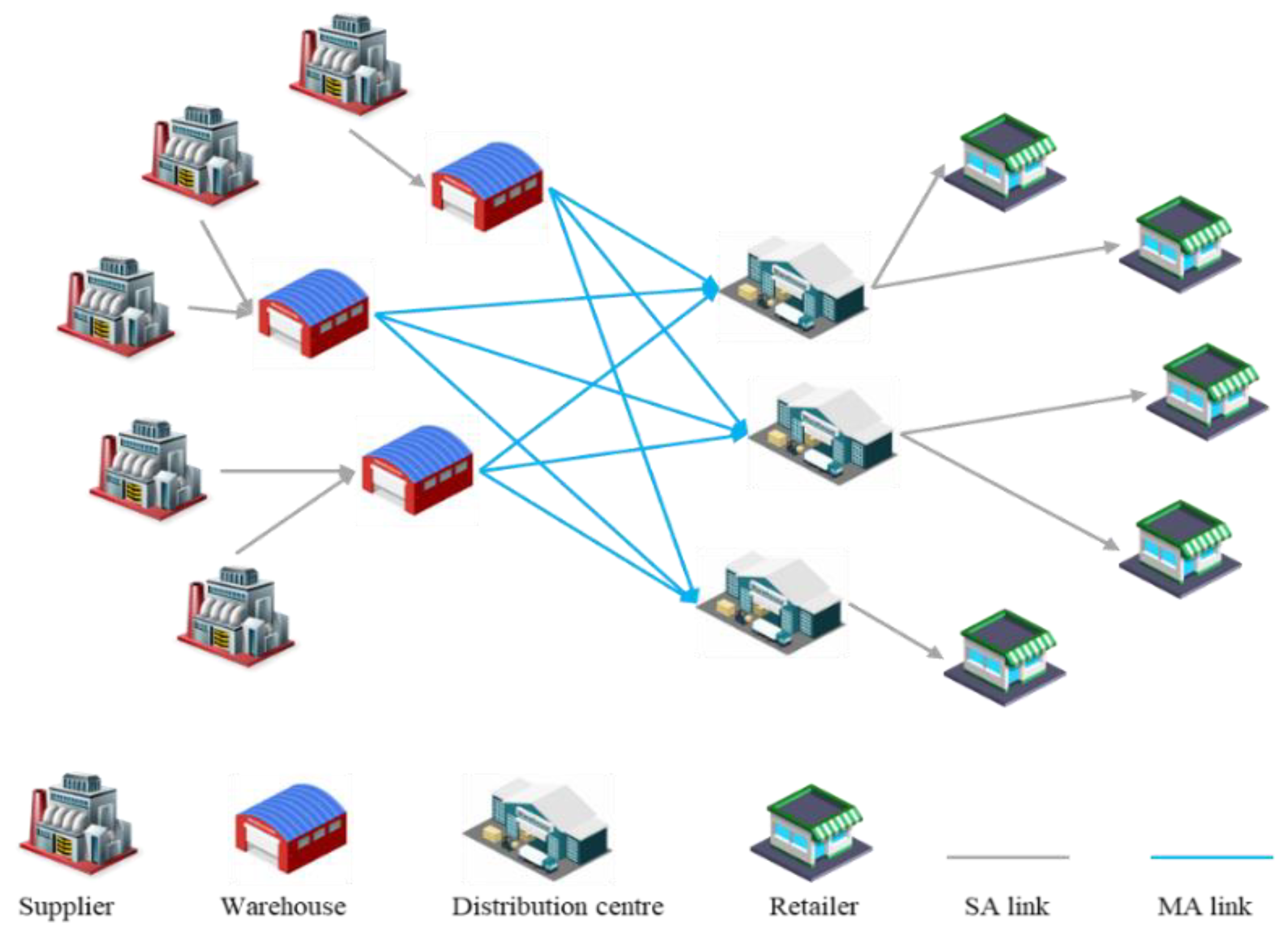
In this paper, we consider a collaborative scenario presented in Figure 1. We assume that each supplier is assigned to a single warehouse (single allocation; SA). In fact, a warehouse can serve multiple distribution centres (multiple allocation; MA), while each retailer can be served only by a single distribution centre (single allocation; SA).

To formulate the studied problem, the following notations are defined:

• T₁: Set of periods; t = 1, …, T₁
• P: Set of products; p = 1, …, P
• N: Set of suppliers; I = 1, …, N
• M: Set of warehouses; m = 1, …, M
• K: Set of distribution centres; k = 1, …, K
• J: Set of retailers; j = 1, …, J
• V: Set of vehicles; v = 1, …, V
• F: Set of nodes F = N${{\displaystyle \cup }}^{ }M{{\displaystyle \cup }}^{ }K{{\displaystyle \cup }}^{ }J$
• H: Set of hubs H = M ${{\displaystyle \cup }}^{ }$ K
• T₂: Set of periods considering the flexibility in the delivery time:
• T₂= T₁ +$\left\{max\left(a^p\right);\forall p\in P\right\}$; t = 1, …, T₂
• A₁: Set of arcs in the upstream part between $N$ and $M$
• A₂: Set of arcs in the midstream part between $M$ and $K$
• A₃: Set of arcs in the downstream part between $K$ and $J$
• A: Set of arcs A = $A_1 {{\displaystyle \cup }}^{ } A_2 {{\displaystyle \cup }}^{ } A_3$

The used parameters as well as the binary and continuous variables are presented in

Table 2. The used parameters as well as the binary and continuous variables.

Notations	Designations	Units
Parameters used for the formulation of the economic indicators
Z	A large constant
$W_{jt}^p$	Quantity of product p requested by the retailer j in period t	Pallets
$S_m^p$	Safety stock of product p in hub m	Pallets
$Q^v$	Vehicle capacity of type v	Pallets
$C_q^v$	Unit transport cost of a fully loaded v-type vehicle	EUR/km
$C_0^v$	Unit transport cost of an empty v-type vehicle	EUR/km
$d_{ij}$	Distances travelled between origin i and destination j	Km
$C{s}_{mt}^p$	Unit storage cost of product p in hub m at period t	EUR/pallet
$C{d}_t^p$	Unit penalty cost of product p at period t	EUR/pallet
$C{w}_m$	Unit opening cost of hubs m	EUR/m2
AP	European pallet surface	m2
$\alpha$	Coefficient greater than or equal to 2
$C{u}^p$	Unit unloading cost of product p	EUR/pallet
$C{l}^p$	Unit loading cost of product p	EUR/pallet
$C{s}^p$	Unit sorting cost of product p	EUR/pallet
Parameters used for the formulation of the environmental indicators
$E_q^v$	Unit CO2 emissions from a fully loaded vehicle of type v	g CO2/km
$E_0^v$	Unit CO2 emissions due to an empty vehicle of type v	g CO2/km
$E{o}_{mt}$	Unit CO2 emissions due to the operation of hubs m at period t	g CO2/KWh
$E{c}_m$	Unit CO2 emissions due to the construction of hubs m	g CO2/m2
$W_{mt}$	Energy consumed by hub m at period t	kwh
$E{M}^v$	CO2 emissions due to the manufacturing of v-type vehicle with depreciation	g CO2
Continuous variables
$q_{ijt}^{pv}$	Quantity of product p transported between origin i and destination j by the v- type vehicle at period t	Pallets
$I_{mt}^p$	Inventory level of product p in hub m at period t	Pallets
$W{d}_t^p$	Quantity of product p delayed in period t	Pallets
$A_m$	Hub m area	m2
$C{T}_{ijt}^v$	Transportation cost between origin i and destination j by v-type vehicle at period t	EUR
$C{S}_{mt}^p$	Storage cost of product p in hub m at period t	EUR
$C{D}_t^p$	Penalty cost of product p at period t	EUR
$C{W}_m$	Opening cost of hubs m	EUR
$C{H}_{mt}^p$	Handling cost of product p in hub m at period t	EUR
CT	Total transportation cost	EUR
CS	Total storage cost	EUR
CO	Total opening cost	EUR
CH	Total handling cost	EUR
CD	Total penalty cost	EUR
$E{V}_{ijt}^v$	CO2 emissions from vehicles moving between origin i and destination j by the v-type vehicle at period t	g CO2
$E{O}_{mt}$	CO2 emissions due to the operation of hubs m at period t	g CO2
$E{C}_m$	CO2 emissions due to the construction of hubs m	g CO2
EV	CO2 emissions from vehicles	g CO2
EC	CO2 emissions due to hub constructions	g CO2
EO	CO2 emissions due to hub operations	g CO2
Discrete variables
$C_m$	Hub m capacity	Pallets
$N_{ijt}^v$	Number of v-type vehicles at period t between origin i and destination j	Vehicles
Binary variables
$y_m$	Is equal to 1 if the hub m is open, and to 0 otherwise
$x_{ij}$	Is equal to 1 if there is a link between the two nodes i and j, and to 0 otherwise
$g_{kj}$	Is equal to 1 if the retailer j is affected to the distribution centre k, and to 0 otherwise

.

The initial model is utilized to minimise two objective functions (F₁ or F₂) representing the economic and environmental aspects of sustainability, respectively. The deterministic mathematical model is formulated as follows:

$$min\left\{F_1;F_2\right\}$$

(1)

$$F_1=CT+CS+CD+CO+CH$$

(2)

$$F_1={\displaystyle \sum }_{\left(i,j\right)\in A,t\in T_2,v\in V}C{T}_{ijt}^v+{\displaystyle \sum }_{m\in W,p\in P,t\in T_2}C{S}_{mt}^p+{\displaystyle \sum }_{p\in P,t\in T_2}C{D}_t^p+{\displaystyle \sum }_{m\in H}C{W}_m+{\displaystyle \sum }_{m\in H,p\in P,t\in T_2}C{H}_{mt}^p$$

(3)

$$C{T}_{ijt}^v=d_{ij}(\frac{C_q^v-C_o^v}{Q^v}.{\displaystyle \sum }_{p\in P}{q}_{ijt}^{pv}+2·C_o^v·N_{ijt}^v);\forall t\in T_2,v\in V,\left(i,j\right)\in A$$

(4)

$$C{S}_{mt}^p=I_{mt}^p·C{s}_m^p;\forall t\in T_2,p\in P,m\in M$$

(5)

$$I_{mt}^p={\displaystyle \sum }_{i\in N,v\in V}{q}_{imt}^{pv}-{\displaystyle \sum }_{k\in K,v\in V}{q}_{mkt}^{pv}+I_{m\left(t-1\right)}^p;\forall t\in T_2,p\in P,m\in M$$

(6)

$$C{D}_t^p=W{d}_t^p·C{d}_t^p;\forall t\in T_2,p\in P$$

(7)

$$W{d}_t^p={\displaystyle \sum }_{j\in J}{W}_{jt}^p-{\displaystyle \sum }_{k\in K,j\in J,v\in V}{q}_{kjt}^{pv}+W{d}_{\left(t-1\right)}^p;\forall t\in T_2,p\in P$$

(8)

$$C{W}_m=A_m·C{w}_m;\forall m\in H$$

(9)

$$A_m=\alpha ·AP.C_m;\forall m\in H$$

(10)

$$C{H}_{mt}^p={\displaystyle \sum }_{i\in \left\{N;M\right\},v\in V}{q}_{imt}^{pv}·c{u}^p+{\displaystyle \sum }_{i\in \left\{N;M\right\},v\in V}{q}_{imt}^{pv}·c{s}^p+{\displaystyle \sum }_{j\in \left\{K;J\right\},v\in V}{q}_{mjt}^{pv}·c{l}^p;\forall t\in T_2,p\in P,m\in H$$

(11)

$$F_2=EV+EO+EC$$

(12)

$$F2={\displaystyle \sum }_{\left(i,j\right)\in A,t\in T_2,v\in V}E{V}_{ijt}^v+{\displaystyle \sum }_{m\in H,t\in T_2}{y}_m·E{O}_{m,t}+{\displaystyle \sum }_{m\in H}E{C}_m$$

(13)

$$E{V}_{ijt}^v=d_{ij}·(\frac{E_q^v-E_o^v}{Q^v}·{\displaystyle \sum }_{p\in P}{q}_{ijt}^{pv}+2·(E_o^v+E{M}^v)·N_{ijt}^v);\forall t\in T_2,v\in V,\left(i,j\right)\in A$$

(14)

$$E{O}_{mt}=E{o}_{mt}·W_{mt};\forall t\in T_2,m\in H$$

(15)

$$E{C}_m=E{c}_m·A_m;\forall m\in H$$

(16)

Subject to

$${\displaystyle \sum }_{i\in N,v\in V}{q}_{imt}^{pv}+I_{m\left(t-1\right)}^p\ge {\displaystyle \sum }_{k\in K,v\in V}{q}_{mkt}^{pv};\forall t\in T_2,m\in M,p\in P$$

(17)

$${\displaystyle \sum }_{m\in M,v\in V}{q}_{mkt}^{pv}={\displaystyle \sum }_{j\in J,v\in V}{q}_{kjt}^{pv};\forall t\in T_2,p\in P,k\in K$$

(18)

$$W_{jt}^p={\displaystyle \sum }_{k\in K,v\in V}{\displaystyle \sum }_{h=1}^{t+a^p}{q}_{kjh}^{pv}-{\displaystyle \sum }_{h=1}^{t-1}{W}_{jh}^p;\forall t\in T_1,p\in P,j\in J$$

(19)

$$S_m^p.y_m\le I_{mt}^p;\forall t\in T_2,p\in P,m\in M$$

(20)

$${\displaystyle \sum }_{i\in \left\{N;M\right\},p\in P,v\in V}{q}_{ijt}^{pv}\le C_j;\forall t\in T_2,\left(i,j\right)\in \left\{A_1,A_2\right\}$$

(21)

$${\displaystyle \sum }_{i\in \left\{N,M\right\}}{x}_{im}\le y_m·Z;\forall m\in \left\{M;K\right\},\left(i,m\right)\in \left\{A_1,A_2\right\}$$

(22)

$$y_m\le {\displaystyle \sum }_{i\in \left\{M;K\right\}}{x}_{im};\forall m\in \left\{M;K\right\},\left(i,m\right)\in \left\{A_1,A_2\right\}$$

(23)

$${\displaystyle \sum }_{m\in \left\{M,K\right\}}{y}_m\le \left\{\left|M\right|;\left|K\right|\right\}$$

(24)

$$q_{imt}^{pv}\le x_{im}·Z;\forall t\in T_2,p\in P,v\in V,\left(i,m\right)\in A$$

(25)

$${\displaystyle \sum }_{m\in M}{x}_{im}=1;\forall i\in N$$

(26)

$${\displaystyle \sum }_{k\in K}{g}_{kj}=1;\forall j\in J$$

(27)

$$q_{kjt}^{pv}\le g_{kj}·Z;\forall t\in T_2,p\in P,v\in V,k\in K,j\in J$$

(28)

$${\displaystyle \sum }_{p\in P}\frac{q_{imt}^{pv}}{Q^v}\le N_{imt}^v;\forall t\in T_2,v\in V,\left(i,m\right)\in A$$

(29)

$$N_{imt}^v\le Nma{x}_{im}^v;\forall t\in T_2,\left(i,m\right)\in A$$

(30)

$${\displaystyle \sum }_{i\in \left\{N;M\right\},v\in V,t\in T_2}{q}_{imt}^{pv}={\displaystyle \sum }_{k\in \left\{K;J\right\},v\in V,t\in T_2}{q}_{mkt}^{pv};\forall \left(i,m\right)\in \left\{A_1,A_2\right\},\left(m,k\right)\in \left\{A_1,A_3\right\},p\in P$$

(31)

$$q_{ijt}^{pv}\ge 0;\forall t\in T_2,\left(i,j\right)\in A,v\in V,p\in P$$

(32)

$$I_{mt}^p\ge 0;\forall t\in T_2,m\in M,p\in P$$

(33)

$$C_m\in \mathbb{N}; \forall m\in H$$

(34)

$$W{d}_t^p\ge 0;\forall t\in T_2,p\in P$$

(35)

$$N_{imt}^v\in \mathbb{N} ;\forall t\in T_2,\left(i,m\right)\in A,v\in V$$

(36)

$$x_{im}\in \left\{0;1\right\};\forall \left(i,m\right)\in A$$

(37)

$$y_m\in \left\{0;1\right\};\forall m\in H$$

(38)

The economic objective function, represented by Equations (2) and (3), minimises the total logistical costs related to five parts: The first part minimises the transportation costs in the upstream, intermediate, and downstream parts of the distribution network. In this part, warehouses and distribution centres are selected to be opened, and non-hub nodes are assigned to the appropriate hubs. Moreover, the optimal quantities transported between the different nodes are determined. In fact, minimising the transportation cost in the downstream part improves the filling rate of vehicles by grouping goods with the same destination in the same vehicles. The second part minimises the cost of storage in warehouses, which guarantees a fast delivery in order to reduce the stock level. The third part reduces the penalty cost due to late delivery by minimising the delayed quantities of goods. The objective is to deliver goods at the right time. The fourth part minimises the costs of opening hubs and, therefore, reduces the number of hubs to be opened and their capacities. The last part’s objective is to reduce the handling costs—namely, the costs of loading, unloading, and sorting. The transportation cost (Equation (4)) depends on the transported quantity, the type of vehicle in use (capacity, unit cost), and the number of required vehicles or trips. The downstream hubs represent the distribution centres with zero storage time, so only upstream hubs are concerned by the storage cost (Equation (5)). The inventory level in warehouse m is represented in Equation (6). The penalty cost (Equation (7)) is evaluated in the last part of the distribution network (distribution centres—retailers), due to delays in some deliveries. The delay in delivering a given quantity of product p in period t is given by Equation (8). The cost of installing a hub m is obtained by Equation (9). The area of the hub m is provided by Equation (10). The hubs’ capacities are considered to be decision variables determined by the model resolution. The handling cost (Equation (11)) concerns the loading, unloading, and sorting operations in the hubs.

The environmental objective function, given by Equations (12) and (13), reduces the different CO₂ emissions due to vehicles and hubs. The vehicle emissions (Equation (14)) are due to two factors—namely, the transportation of goods, and the depreciation of vehicles. As with the transportation cost, minimising the vehicles’ CO₂ emissions allows us to determine the optimal quantities to transport, select the appropriate hubs to be opened, and assign non-hub nodes to the appropriate hubs. The CO₂ emissions depend on the amount of the carried goods and the type of vehicle used (capacity and unit cost). In addition, the CO₂ emissions from the shared warehouses are also classified into two categories: those due to the hubs’ operations (Equation (15)), and those resulting from their construction (Equation (16)). Reducing these types of emissions reduces the number and the capacity of hubs to be opened. The quantity of CO₂ emissions released by each material is calculated based on [33].

Equation (17) ensures that the sum of the quantities delivered by the suppliers in period t and the inventory level of the previous period (t − 1) is greater than the quantity of goods delivered between the hubs. As there is no storage in the distribution centres, Equation (18) guarantees that the quantity of goods delivered from warehouse m to distribution centre k in period t is exactly equal to the quantity delivered to the customers, while considering the transport time. The demand for product p by the customer j in period t is delivered at most in period (t + a^p) thanks to Equation (19), where a^p denotes the number of periods allowed to deliver the requested quantity. According to Equation (20), the inventory level of each product in the upstream hubs is always higher than the safety stock. Equation (21) ensures that when hubs m or k are open, their capacities are higher than the quantity of the incoming goods. Equations (22) and (23) indicate that a warehouse is only open if at least one supplier is assigned to it, and that a distribution centre is only open when there is a warehouse assigned to it. Equation (24) limits the number of upstream and downstream hubs to be opened. Equation (25) limits the flow on the arcs (there are no goods transported between unlinked nodes). Every supplier can only deliver to one shared warehouse, which is guaranteed by Equation (26). Equation (27) ensures that a retailer can only be assigned to one distribution centre. Equation (28) indicates that each distribution centre k can only deliver to one retailer j when it is assigned to it. Equation (29) determines the number of vehicles required in the three parts of the distribution network for each period and for each type of vehicle. Equation (30) is used to limit the maximum number of vehicles or trips for each vehicle type. Equation (31) is a flow conservation equation. Finally, Equations (32)–(38) define the domain of each decision variable.

3.1. Demand Uncertainty

Customer demand cannot be estimated since, during the COVID-19 pandemic, some companies have had a large variation in demand (decrease or increase in sales). Therefore, they are given in the form of interval values. For each retailer $j\in J$, period $t\in T_2$, and product $p\in P$, the demand $W_{jt}^p\in \left[W_{jt}^{pL}, W_{jt}^{pL}+W_{jt}^{p\Delta }\right]$, where $W_{jt}^{pL}$ is its nominal value and $W_{jt}^{p\Delta }\ge 0$ designates its deviation. The parameter $S_w$ denotes a subset of uncertain demands, and was defined by [16] as follows:

$$S_w=\{w:W_{jt}^p\in \left[W_{jt}^{pL},W_{jt}^{pL}+W_{jt}^{p\Delta }\right];\forall j\in J,t\in T_2,p\in P\}$$

The uncertainty budget, chosen by decision-makers, is $h_w\in \left[0, 1\right]$; it limits the number of demands that can deviate from their nominal values. This condition is justified by the fact that all parameters rarely deviate from their nominal values. Therefore, the adjustment of this parameter provides some flexibility for decision-makers to choose more or less conservative solutions [34].

The mathematical model with the economic objective of a robust collaborative distribution network design problem with uncertain demands is as follows:

$$min\left\{CT+CS+CO+CH+{\displaystyle \sum }_{t\in T_2,p\in P}(W{d}_{\left(t-1\right)}^p-{\displaystyle \sum }_{k\in K,j\in J,v\in V}{q}_{kjt}^{pv}).C{d}_t^p+{\displaystyle \sum }_{t\in T_2,p\in P}{\displaystyle \sum }_{j\in J}{W}_{jt}^{pL}.C{d}_t^p+ma{x}_{S_w:\left|S_w\right|\le h_w}\left\{{\displaystyle \sum }_{t\in T_2,p\in P}{\displaystyle \sum }_{j\in J}{W}_{jt}^{p\Delta }.C{d}_t^p\right\}\right\}$$

(39)

Subject to (17), (18), (20)–(38)

$$W_{jt}^{pL}+{\displaystyle \sum }_{h=1}^{t-1}{W}_{jh}^{pL}+ma{x}_{S_w:\left|S_w\right|\le h_w}\left\{W_{jt}^{p\Delta }+{\displaystyle \sum }_{h=1}^{t-1}{W}_{jh}^{p\Delta }\right\}={\displaystyle \sum }_{k\in K,v\in V}{\displaystyle \sum }_{h=1}^{t+a^p}{q}_{kjh}^{pv};\forall t\in T_1,p\in P,j\in J$$

(40)

$$W{d}_t^p={\displaystyle \sum }_{j\in J}{W}_{jt}^{pL}+ma{x}_{S_w:\left|S_w\right|\le h_w}\left\{{\displaystyle \sum }_{j\in J}{W}_{jt}^{p\Delta }\right\}-{\displaystyle \sum }_{k\in K,j\in J,v\in V}{q}_{kjt}^{pv}+W{d}_{\left(t-1\right)}^p;\forall t\in T_2,p\in P$$

(41)

The objective of the inner maximisation of the objective function is to select the subset S_w such that the perturbations increase the penalty cost. The binary variables $u_{jt}^p\in \left\{0,1\right\}$, $v_{jt}^p\in \left\{0,1\right\},$ and $l_{jt}^p\in \left\{0,1\right\}$ for each retailer $j\in J$, product $p\in P,$ and period $t\in T_2$ are defined to reformulate the previously applied model as follows:

$$min\left\{CT+CS+CO+CH+{\displaystyle \sum }_{t\in T_2,p\in P}(W{d}_{\left(t-1\right)}^p-{\displaystyle \sum }_{k\in K,j\in J,v\in V}{q}_{kjt}^{pv}).C{d}_t^p+{\displaystyle \sum }_{t\in T_2,p\in P}{\displaystyle \sum }_{j\in J}{W}_{jt}^{pL}.C{d}_t^p+max\left\{{\displaystyle \sum }_{t\in T_2,p\in P}{\displaystyle \sum }_{j\in J}{W}_{jt}^{p\Delta }.C{d}_t^p.u_{jt}^p\right\}\right\}$$

(42)

Subject to Equations (17), (18), and (20)–(38):

$${\displaystyle \sum }_{t\in T_2,p\in P}{\displaystyle \sum }_{j\in J}{u}_{jt}^p\le h_w$$

(43)

$$0\le u_{jt}^p\le 1;\forall j\in J,p\in P,t\in T_2$$

(44)

$$W_{jt}^{pL}+{\displaystyle \sum }_{h=1}^{t-1}{W}_{jh}^{pL}+max\left\{W_{jt}^{p\Delta }.v_{jt}^p+{\displaystyle \sum }_{h=1}^{t-1}{W}_{jh}^{p\Delta }.v_{jh}^p\right\}={\displaystyle \sum }_{k\in K,v\in V}{\displaystyle \sum }_{h=1}^{t+a^p}{q}_{kjh}^{pv}\forall t\in T_1,p\in P,j\in J$$

(45)

$${\displaystyle \sum }_{j\in J}{\displaystyle \sum }_{t\in T_2,p\in P}{v}_{jt}^p\le h_w$$

(46)

$${\displaystyle \sum }_{h=1}^{t-1}{\displaystyle \sum }_{j\in J}{\displaystyle \sum }_{p\in P}{v}_{jh}^p\le h_w$$

(47)

$$0\le v_{jt}^p\le 1;\forall j\in J,p\in P,t\in T_2$$

(48)

$$0\le v_{jh}^p\le 1;\forall j\in J,p\in P,h\in \left[1,t-1\right]$$

(49)

$$W{d}_t^p={\displaystyle \sum }_{j\in J}{W}_{jt}^{pL}+max\left\{{\displaystyle \sum }_{j\in J}{W}_{jt}^{p\Delta }.l_{jt}^p\right\}-{\displaystyle \sum }_{k\in K,v\in V,j\in J}{q}_{kjt}^{pv}+W{d}_{\left(t-1\right)}^p;\forall t\in T_2,p\in P$$

(50)

$${\displaystyle \sum }_{j\in J}{\displaystyle \sum }_{t\in T_2,p\in P}{l}_{jt}^p\le h_w$$

(51)

$$0\le l_{jt}^p\le 1;\forall j\in J,p\in P,t\in T_2$$

(52)

where Equations (43), (44), (46)–(49), (51) and (52) ensure that at most h_w coefficients $W_{jt}^p$ are allowed to change. Note that in the last model, the requirement that the variables $u_{jt}^p$, $v_{jt}^p$, and $l_{jt}^p$ are binary can be relaxed. The resulting linear program will have the same optimal solution as the initial binary program.

Taking the dual variables of the above-cited problem, the robust collaborative DNDP under the budget demand uncertainty can be formulated by the following MILP model:

$$min\left\{CT+CS+CO+CH+{\displaystyle \sum }_{t\in T_2,p\in P}\left(W{d}_{\left(t-1\right)}^p-{\displaystyle \sum }_{k\in K,v\in V,j\in J}{q}_{kjt}^{pv}\right)·C{d}_t^p+{\displaystyle \sum }_{j\in J}{\displaystyle \sum }_{t\in T_2,p\in P}({\lambda }_{jt}^p+W_{jt}^{pL}·C{d}_t^p)+h_w·\mu \right\}$$

(53)

Subject to Equations (17), (18), and (20–38):

$${\lambda }_{jt}^p+\mu \ge W_{jt}^{p\Delta }·C{d}_t^p;\forall t\in T_2,p\in P,j\in J$$

(54)

$$\mu ,{\lambda }_{jt}^p\ge 0;\forall t\in T_2,p\in P,j\in J$$

(55)

$$W_{jt}^{pL}+{\displaystyle \sum }_{h=1}^{t-1}{W}_{jh}^{pL}+{\beta }_{jt}^p+{\displaystyle \sum }_{h=1}^{t-1}{\beta }_{jh}^p+\gamma ·h_w={\displaystyle \sum }_{k\in K,v\in V}{\displaystyle \sum }_{h=1}^{t+a^p}{q}_{kjh}^{pv};\forall t\in T_1,p\in P,j\in J$$

(56)

$$\gamma +{\beta }_{jt}^p+{\displaystyle \sum }_{h=1}^{t-1}{\beta }_{jh}^p\ge W_{jt}^{p\Delta }+{\displaystyle \sum }_{h=1}^{t-1}{W}_{jh}^{p\Delta };\forall t\in T_2,p\in P,j\in J$$

(57)

$$\gamma ,{\beta }_{jt}^p\ge 0;\forall t\in T_2,p\in P,j\in J$$

(58)

$$W{d}_t^p={\displaystyle \sum }_{j\in J}{W}_{jt}^{pL}+{\displaystyle \sum }_j{\Gamma }_{jt}^p+\alpha ·h_w-{\displaystyle \sum }_{j\in J,k\in K,v\in V}{q}_{kjt}^{pv}+W{d}_{\left(t-1\right)}^p;\forall t\in T_2, p\in P$$

(59)

$${\Gamma }_{jt}^p+\alpha \ge W_{jt}^{p\Delta };\forall t\in T_2,p\in P,j\in J$$

(60)

$$\alpha ,{\Gamma }_{jt}^p\ge 0;\forall t\in T_2,p\in P,j\in J$$

(61)

where the $\mu$,${\lambda }_{jt}^p$,$\gamma$,${\beta }_{jt}^p$, $\alpha ,$ and ${\Gamma }_{jt}^p$ are the dual variables associated with Equations (43), (44) and (46)–(52), respectively.

3.2. Unit Transportation Costs Uncertainty

Unit transportation costs vary depending on the fluctuating price of fuel, according to several external factors, such as geopolitical tensions, epidemics, and global growth. For each vehicle $v\in V$, the unit transportation cost for a fully loaded vehicle $C_q^v\in \left[C_q^{vL},C_q^{vL}+C_q^{v\Delta }\right]$, where $C_q^{vL}$ is its nominal value and $C_q^{v\Delta }\ge 0$ is its deviation, while the unit transportation cost for an empty vehicle $C_0^v\in \left[C_0^{vL},C_0^{vL}+C_0^{v\Delta }\right]$, where $C_0^{vL}$ is its nominal value and $C_0^{v\Delta }\ge 0$ is its deviation. The parameters $S_{Cq}$ and $S_{C0}$ denote the subsets of uncertain unit transportation costs with full and empty vehicles, respectively; they are defined as follows:

$S_{Cq}=\left\{C_q:W_{jt}^p\in \left[C_q^{vL},C_q^{vL}+C_q^{v\Delta }\right];\forall v\in V\right\}$ and $S_{C0}=\left\{C_q:W_{jt}^p\in \left[C_0^{vL},C_0^{vL}+C_0^{v\Delta }\right];\forall v\in V\right\}$. The uncertainty budgets are: $h_{C_q}\in \left[0,1\right]$ and $h_{C_0}\in \left[0,1\right]$.

First, we define the following two variables:

$$C_1^v={\displaystyle \sum }_{\left(i,j\right)\in A,t\in T_2}{d}_{ij} ·{\displaystyle \sum }_{p\in P}{q}_{ijt}^{pv};\forall v\in V$$

(62)

$$C_2^v={\displaystyle \sum }_{i\left(i,j\right)\in A,t\in T_2}{d}_{ij}\left(2 ·N_{ijt}^v-\frac{1}{Q^v}{\displaystyle \sum }_{p\in P}{q}_{ijt}^{pv}\right);\forall v\in V$$

(63)

The mathematical model with the economic objective of a robust collaborative distribution network design problem with uncertain unit transportation costs is formulated as follows:

$$min\left\{CS+CD+CO+CH+{\displaystyle \sum }_{v\in V}{C}_q^{vL}·C_1^v+{\displaystyle \sum }_{v\in V}{C}_0^{vL}·C_2^v+ma{x}_{S_{Cq}:\left|S_{Cq}\right|\le h_{Cq}}\left\{{\displaystyle \sum }_{v\in V}{C}_q^{v\Delta }·C_1^v\right\}+ma{x}_{S_{C0}:\left|S_{C0}\right|\le h_{C0}}\left\{{\displaystyle \sum }_{v\in V}{C}_0^{v\Delta }·C_2^v\right\}\right\}$$

(64)

Subject to Equations (17)–(38).

The objective of the inner maximization of the objective function is to select the subsets $S_{C_q}$ and $S_{C_0}$ such that the perturbations $C_q^{v\Delta }$ and $C_0^{v\Delta }$ increase the transportation cost. The binary variables $u^v\in \left\{0, 1\right\}$ and $l^v\in \left\{0, 1\right\}$ for each vehicle $v\in V$ are defined to reformulate the previous model as follows:

$$min\left\{CS+CD+CO+CH+{\displaystyle \sum }_{v\in V}{C}_q^{vL}.C_1^v+{\displaystyle \sum }_{v\in V}{C}_0^{vL}.C_2^v+max\left\{{\displaystyle \sum }_{v\in V}{C}_q^{v\Delta }.C_1^v.u^v\right\}+max\left\{{\displaystyle \sum }_{v\in V}{C}_0^{v\Delta }.C_2^v.l^v\right\}\right\}$$

(65)

Subject to Equations (17)–(38):

$${\displaystyle \sum }_{v\in V}{u}^v\le h_{Cq}$$

(66)

$${\displaystyle \sum }_{v\in V}{l}^v\le h_{C0}$$

(67)

$$u^v\in \left\{0, 1\right\};\forall v\in V$$

(68)

$$l^v\in \left\{0,1\right\};\forall v\in V$$

(69)

Equations (66) and (68) ensure that at most $h_{Cq}$ coefficients $C_q^v$ are allowed to change, while Equations (67) and (69) apply to the $h_{C0}$ and $C_0^v$ case. Note that, in the last model, the requirement that the variables $u^v$ and $l^v$ are binary can be relaxed. The resulting linear program will have the same optimal solution as the initial binary program.

As with the uncertain demands case, the robust collaborative DNDP under the budget unit transportation costs uncertainty can be formulated as follows:

$$min\left\{CS+CD+CO+CH+{\displaystyle \sum }_{v\in V}{C}_q^{vL}·C_1^v+{\displaystyle \sum }_{v\in V}{C}_0^{vL}·C_2^v+{\displaystyle \sum }_{v\in V}{\lambda }^v+h_{Cq}·\mu +{\displaystyle \sum }_{v\in V}{\beta }^v+h_{C0}·\Gamma \right\}$$

(70)

Subject to Equations (17)–(38):

$${\lambda }^v+\mu \ge C_q^{v\Delta }·C_1^v;\forall v\in V$$

(71)

$${\beta }^v+\Gamma \ge C_0^{v\Delta }·C_2^v;\forall v\in V$$

(72)

$$\mu ,{\lambda }^v\ge 0;\forall v\in V$$

(73)

$$\Gamma ,{\beta }^v\ge 0;\forall v\in V$$

(74)

where $\mu$, ${\lambda }^v$, $\Gamma ,$ and ${\beta }^v$ are the dual variables associated with Equations (66)–(68) and (70), respectively.

To linearise Equations (71) and (72), we use McCormick envelopes, so we obtain the following model:

$$min\left\{CS+CD+CO+CH+{\displaystyle \sum }_{v\in V}{A}^v+{\displaystyle \sum }_{v\in V}{B}^v+{\displaystyle \sum }_{v\in V}{\lambda }^v+h_{Cq}·\mu +{\displaystyle \sum }_{v\in V}{\beta }^v+h_{C0}·\Gamma \right\}$$

(75)

Subject to Equations (17)–(38), (73) and (74):

$${\lambda }^v+\mu \ge A^v;\forall v\in V$$

(76)

$${\beta }^v+\Gamma \ge B^v;\forall v\in V$$

(77)

$$0\le C_q^{v\Delta }\le C_q^{vL};\forall v\in V$$

(78)

$$0\le C_1^v\le C_{1\mathrm{upper}}^v;\forall v\in V$$

(79)

$$0\le C_0^{v\Delta }\le C_0^{vL};\forall v\in V$$

(80)

$$0\le C_2^v\le C_{2\mathrm{upper}}^v;\forall v\in V$$

(81)

$$A^v\ge C_q^{vL}·C_1^v+C_{1\mathrm{upper}}^v·C_q^{v\Delta }-C_{1\mathrm{upper}}^v·C_q^{vL} ;\forall v\in V$$

(82)

$$A^v\ge 0 ;\forall v\in V$$

(83)

$$A^v\le C_q^{vL}·C_1^v ;\forall v\in V$$

(84)

$$A^v\le C_{1\mathrm{upper}}^v·C_q^{v\Delta } ;\forall v\in V$$

(85)

$$B^v\ge C_0^{vL}·C_2^v+C_{2\mathrm{upper}}^v·C_0^{v\Delta }-C_{2\mathrm{upper}}^v·C_0^{vL };\forall v\in V$$

(86)

$$B^v\ge 0 ;\forall v\in V$$

(87)

$$B^v\le C_0^{vL}·C_2^v ;\forall v\in V$$

(88)

$$B^v\le C_{2\mathrm{upper}}^v·C_0^{v\Delta } ;\forall v\in V$$

(89)

where we use $A^v=C_q^{v\Delta }·C_1^v$ and $B^v=C_0^{v\Delta }·C_2^v$. Moreover, $C_{1\mathrm{upper}}^v$ and $C_{2\mathrm{upper}}^v$ are the upper bounds for $C_1^v$ and $C_2^v$, respectively.

3.3. Maximum Number of Vehicles in Use Uncertainty

Vehicles may break down during some periods, and sometimes a driver can be absent (unexpected illness, etc.). Therefore, the maximum number of vehicles in use is uncertain. For each vehicle $v\in V$, arc $\left(i,m\right)\in A$, and period $t\in T_2$, the maximum number of vehicles in use = $Nma{x}_{im}^v\in \left[Nma{x}_{im}^{vL}-Nma{x}_{im}^{v\Delta },Nma{x}_{im}^{vL}\right],$ where $Nma{x}_{im}^{v\Delta }$ is its nominal value and $Nma{x}_{im}^{v\Delta }\ge 0$ corresponds to its deviation. The parameter $S_n$ denotes the subset of the maximum number of vehicles in use that is uncertain; it is defined as follows:

$$S_n=\left\{N_{max}:Nma{x}^v\in \left[Nma{x}_{im}^{vL}-Nma{x}_{im}^{v\Delta },Nma{x}_{im}^{vL}\right];\forall t\in T_2,\left(i,m\right)\in A,v\in V\right\}$$

The uncertainty budget is $h_n\in \left[0, 1\right]$.

The mathematical model with the economic objective of a robust collaborative distribution network design problem with uncertain maximum number of vehicles in use is presented below:

$$min{F}_1=min\{{\displaystyle \sum }_{a\in A,v\in V,t\in T_2}C{T}_{at}^v+{\displaystyle \sum }_{t\in T_2,m\in M,p\in P}C{S}_{mt}^p+{\displaystyle \sum }_{t\in T_2,p\in P}C{D}_t^p+{\displaystyle \sum }_{m\in H}C{W}_m+{\displaystyle \sum }_{m\in H,p\in P,t\in T_2}C{H}_{mt}^p\}$$

(90)

Subject to Equations (17)–(28) and (30)–(38):

$$N_{imt}^v\le Nma{x}_{im}^{vL}-ma{x}_{S_n:\left|S_n\right|\le h_n}\left\{Nma{x}_{im}^{v\Delta }\right\};\forall t\in T_2,\left(i,m\right)\in A,v\in V$$

(91)

The objective of the inner maximization of the objective function is to select the subset $S_n$ such that the perturbations $Nma{x}_{im }^{v\Delta }$ increase the number of vehicles in use subtracted from the total maximum number of these vehicles. The binary variable $f^v\in \left\{0, 1\right\}$ for each vehicle $v\in V$ is defined to reformulate the previously applied model, as follows:

$$min{F}_1=min\{{\displaystyle \sum }_{a\in A,v\in V,t\in T_2}C{T}_{at}^v+{\displaystyle \sum }_{t\in T_2,m\in M,p\in P}C{S}_{mt}^p+{\displaystyle \sum }_{t\in T_2,p\in P}C{D}_t^p+{\displaystyle \sum }_{m\in H}C{W}_m+{\displaystyle \sum }_{m\in H,p\in P,t\in T_2}C{H}_{mt}^p\}$$

Subject to Equations (17)–(28) and (30)–(38):

$$N_{imt}^v\le Nma{x}_{im}^{vL}-max\left\{Nma{x}_{im}^{v\Delta }·f^v\right\};\forall t\in T_2,\left(i,m\right)\in A,v\in V$$

(92)

$${\displaystyle \sum }_{v\in V}{f}^v\le h_n$$

(93)

$$f^v\in \left\{0, 1\right\};\forall v\in V$$

(94)

where Equations (93) and (94) ensure that at most $h_n$ coefficients $Nma{x}_{im}^v$ are allowed to change. Note that, in the last model, the requirement that the variable $f^v$ is binary can be relaxed. The resulting linear program will have the same optimal solution as the initial binary program.

As with the previous cases of demands and unit transportation cost uncertainties, the robust collaborative DNDP under the uncertainty of the maximum number of vehicles in use can be formulated by the following MILP model:

$$min{F}_1=min\{{\displaystyle \sum }_{a\in A,v\in V,t\in T_2}C{T}_{at}^v+{\displaystyle \sum }_{t\in T_2,m\in M,p\in P}C{S}_{mt}^p+{\displaystyle \sum }_{t\in T_2,p\in P}C{D}_t^p+{\displaystyle \sum }_{m\in H}C{W}_m+{\displaystyle \sum }_{m\in H,p\in P,t\in T_2}C{H}_{mt}^p\}$$

Subject to Equations (17)–(28) and (30)–(38):

$$N_{imt}^v\le Nma{x}_{im}^{vL}-{\lambda }^v-\beta ·h_n;\forall t\in T_2,\left(i,m\right)\in A,v\in V$$

(95)

$${\lambda }^v+\beta \ge Nma{x}_{im}^{v\Delta };\forall v\in V, \left(i,m\right)\in A$$

(96)

$$\beta ,{\lambda }^v\ge 0;\forall v\in V$$

(97)

where $\beta$ and ${\lambda }^v$ are the dual variables associated with Equations (93) and (94), respectively.

3.4. Uncertainty of Demands, Unit Transportation Costs, and Maximum Number of Vehicles in Use

In this subsection, we focus on the case where the demands, unit transportation costs, and maximum number of vehicles are uncertain. As with the previous cases, the demand $W_{jt}^p\in \left[W_{jt}^{pL}, W_{jt}^{pL}+W_{jt}^{p\Delta }\right]$, the unit transportation cost of a full vehicle $C_q^v\in \left[C_q^{vL}, C_q^{vL}+C_q^{v\Delta }\right]$, the unit transportation cost of an empty vehicle $C_0^v\in \left[C_0^{vL}, C_0^{vL}+C_0^{v\Delta }\right]$, the maximum number of vehicles in use $Nma{x}^v\in \left[Nma{x}_{im}^{vL}-Nma{x}_{im}^{v\Delta }, Nma{x}_{im}^{vL}\right]$, and $h_w$, $h_{C_q}$, $h_{C_0}$, and $h_n$ are the uncertainty budgets of each uncertain parameter.

We use the already-introduced variables $C_1^v$ and $C_2^v$ in the unit transportation costs uncertainty case. The uncertainty does not influence the environmental objective function. Therefore, the resulting mathematical model is formulated as follows:

$$\begin{array}{l}Min\{CS+CO+CH+{\displaystyle {\displaystyle \sum }_{v\in V}}{C}_q^{vL}·C_1^v+{\displaystyle {\displaystyle \sum }_{v\in V}}{C}_0^{vL}·C_2^v+ma{x}_{S_{Cq}:\left|S_{Cq}\right|\le h_{Cq}}\left\{{\displaystyle {\displaystyle \sum }_{v\in V}}{C}_q^{v\Delta }·C_1^v\right\}\\ +ma{x}_{S_{C0}:\left|S_{C0}\right|\le h_{C0}}\left\{{\displaystyle {\displaystyle \sum }_{v\in V}}{C}_0^{v\Delta }·C_2^v\right\}+{\displaystyle {\displaystyle \sum }_{t\in T_2,p\in P}}(W{d}_{\left(t-1\right)}^p-{\displaystyle {\displaystyle \sum }_{k\in K,j\in J,v\in V}}{q}_{kjt}^{pv})·C{d}_t^p\\ +{\displaystyle {\displaystyle \sum }_{t\in T_2,p\in P}}{\displaystyle {\displaystyle \sum }_{j\in J}}{W}_{jt}^{pL}.C{d}_t^p+ma{x}_{S_w:\left|S_w\right|\le h_w}\left\{{\displaystyle {\displaystyle \sum }_{t\in T_2,p\in P}}{\displaystyle {\displaystyle \sum }_{j\in J}}{W}_{jt}^{p\Delta }·C{d}_t^p\right\}\}\end{array}$$

(98)

Subject to Equations (17), (18), (20)–(38), (40), (41) and (91):

To reformulate this inner problem as a mathematical program, we introduce the binary variables ${\alpha }_{jt}^p\in \left\{0,1\right\}$, ${\beta }_{jt}^p\in \left\{0,1\right\}$, and ${\gamma }_{jt}^p\in \left\{0,1\right\}$ for each retailer $j\in J$, product $p\in P,$ and period $t\in T_2$; and $a^v \in \left\{0,1\right\}$, $b^v \in \left\{0,1\right\}$, and $d^v \in \left\{0,1\right\}$ for each vehicle $v\in V$.

Consequently, the following model is obtained:

$$\begin{array}{l}Min\{CT+CS+CO+CH+{\displaystyle {\displaystyle \sum }_{t\in T_2,p\in P}}(W{d}_{\left(t-1\right)}^p-{\displaystyle {\displaystyle \sum }_{k\in K,j\in J,v\in V}}{q}_{kjt}^{pv})·C{d}_t^p+{\displaystyle {\displaystyle \sum }_{t\in T_2,p\in P}}{\displaystyle {\displaystyle \sum }_j}{W}_{jt}^{pL}·C{d}_t^p\\ +max\left\{{\displaystyle {\displaystyle \sum }_{t\in T_2,p\in P}}{\displaystyle {\displaystyle \sum }_j}{W}_{jt}^{p\Delta }·C{d}_t^p.{\alpha }_{jt}^p\right\}+{\displaystyle {\displaystyle \sum }_{v\in V}}{C}_q^{vL}·C_1^v+{\displaystyle {\displaystyle \sum }_{v\in V}}{C}_0^{vL}·C_2^v+max\left\{{\displaystyle {\displaystyle \sum }_{v\in V}}{C}_q^{v\Delta }·C_1^v{a}^v\right\}\\ +max\left\{{\displaystyle {\displaystyle \sum }_{v\in V}}{C}_0^{v\Delta }·C_2^v·b^v\right\}\}\end{array}$$

(99)

Subject to Equations (17), (18) and (20)–(38):

$${\displaystyle \sum }_{t\in T_2,p\in P}{\displaystyle \sum }_{j\in J}{\alpha }_{jt}^p\le h_w;\forall j\in J,p\in P,t\in T_2$$

(100)

$$0\le {\alpha }_{jt}^p\le 1;\forall j\in J,p\in P,t\in T_2$$

(101)

$$W_{jt}^{pL}+{\displaystyle \sum }_{h=1}^{t-1}{W}_{jh}^{pL}+max\left\{W_{jt}^{p\Delta }·{\beta }_{jt}^p+{\displaystyle \sum }_{h=1}^{t-1}{W}_{jh}^{p\Delta }·{\beta }_{jh}^p\right\}={\displaystyle \sum }_{k\in K,v\in V}{\displaystyle \sum }_{h=1}^{t+a^p}{q}_{kjh}^{pv};\forall t\in T_1, tp\in P,j\in J$$

(102)

$${\displaystyle \sum }_{j\in J}{\displaystyle \sum }_{t\in T_2,p\in P}{\beta }_{jt}^p\le h_w$$

(103)

$${\displaystyle \sum }_{h=1}^{t-1}{\displaystyle \sum }_{j\in J}{\displaystyle \sum }_{p\in P}{\beta }_{jh}^p\le h_w$$

(104)

$$0\le {\beta }_{jt}^p\le 1;\forall j\in J,p\in P,t\in T_2$$

(105)

$$0\le {\beta }_{jh}^p\le 1;\forall j\in J,p\in P,h\in \left[1;t-1\right]$$

(106)

$$W{d}_t^p={\displaystyle \sum }_{j\in J}{W}_{jt}^{pL}+max\left\{{\displaystyle \sum }_{j\in J}{W}_{jt}^{p\Delta }.{\gamma }_{jt}^p\right\}-{\displaystyle \sum }_{k\in K,v\in V,j\in J}{q}_{kjt}^{pv}+W{d}_{\left(t-1\right)}^p;\forall t\in T_2,p\in P$$

(107)

$${\displaystyle \sum }_{j\in J}{\displaystyle \sum }_{t\in T_2,p\in P}{\gamma }_{jt}^p\le h_w$$

(108)

$$0\le {\gamma }_{jt}^p\le 1;\forall j\in J,p\in P,t\in T_2$$

(109)

$${\displaystyle \sum }_{v\in V}{a}^v\le h_{Cq}$$

(110)

$$a^v\ge 0;\forall v\in V$$

(111)

$${\displaystyle \sum }_{v\in V}{b}^v\le h_{C0}$$

(112)

$$b^v\ge 0;\forall v\in V$$

(113)

$$N_{imt}^v\le Nma{x}_{im}^{vL}-max\left\{Nma{x}_{im}^{v\Delta }·d^v\right\};\forall t\in T_2,\left(i,m\right)\in A,v\in V$$

(114)

$${\displaystyle \sum }_{v\in V}{d}^v\le h_n$$

(115)

$$d^v\ge 0;\forall v\in V$$

(116)

The obtained linear problem is written as follows:

$$\begin{array}{l}Min\{CS+CO+CH+{\displaystyle {\displaystyle \sum }_{v\in V}}{D}^v+{\displaystyle {\displaystyle \sum }_{v\in V}}{F}^v+{\displaystyle {\displaystyle \sum }_{v\in V}}{\pi }^v+h_{Cq}·\rho +{\displaystyle {\displaystyle \sum }_{v\in V}}{\sigma }^v+h_{C0}·\tau \\ +{\displaystyle {\displaystyle \sum }_{t\in T_2,p\in P}}\left(W{d}_{\left(t-1\right)}^p-{\displaystyle {\displaystyle \sum }_{k\in K,j\in J,v\in V}}{q}_{kjt}^{pv}\right)·C{d}_t^p+{\displaystyle {\displaystyle \sum }_{j\in J}{\displaystyle {\displaystyle \sum }_{t\in T_2,p\in P}}}({\delta }_{jt}^p+W_{jt}^{pL}·C{d}_t^p)+h_w·\epsilon \}\end{array}$$

(117)

Subject to Equations (17), (18) and (20)–(38):

$${\pi }^v+\rho \ge D^v;\forall v\in V$$

(118)

$${\sigma }^v+\tau \ge F^v;\forall v\in V$$

(119)

$${\pi }^v,{\sigma }^v,\rho ,\tau \ge 0;\forall v\in V$$

(120)

$$0\le C_q^{v\Delta }\le C_q^{vL};\forall v\in V$$

(121)

$$0\le C_1^v\le C_{1\mathrm{upper}}^v;\forall v\in V$$

(122)

$$0\le C_0^{v\Delta }\le C_0^{vL};\forall v\in V$$

(123)

$$0\le C_2^v\le C_{2\mathrm{upper}}^v;\forall v\in V$$

(124)

$$D^v\ge C_q^{vL}·C_1^v+C_{1\mathrm{upper}}^v.C_q^{v\Delta }-C_{1\mathrm{upper}}^v·C_q^{vL} ;\forall v\in V$$

(125)

$$D^v\ge 0 ;\forall v\in V$$

(126)

$$D^v\le C_q^{vL}·C_1^v ;\forall v\in V$$

(127)

$$D^v\le C_{1\mathrm{upper}}^v·C_q^{v\Delta } ;\forall v\in V$$

(128)

$$F^v\ge C_0^{vL}·C_2^v+C_{2\mathrm{upper}}^v·C_0^{v\Delta }-C_{2\mathrm{upper}}^v·C_0^{vL };\forall v\in V$$

(129)

$$F^v\ge 0 ;\forall v\in V$$

(130)

$$F^v\le C_0^{vL}·C_2^v ;\forall v\in V$$

(131)

$$F^v\le C_{2\mathrm{upper}}^v ·C_0^{v\Delta } ;\forall v\in V$$

(132)

$${\delta }_{jt}^p+\epsilon \ge W_{jt}^{p\Delta }·C{d}_t^p;\forall t\in T_2,p\in P,j\in J$$

(133)

$${\delta }_{jt}^p,\epsilon \ge 0;\forall t\in T_2,p\in P,j\in J$$

(134)

$$W_{jt}^{pL}+{\displaystyle \sum }_{h=1}^{t-1}{W}_{jh}^{pL}+{\xi }_{jt}^p+{\displaystyle \sum }_{h=1}^{t-1}{\xi }_{jh}^p+\theta ·h_w={\displaystyle \sum }_{k\in K,v\in V}{\displaystyle \sum }_{h=1}^{t+a^p}{q}_{kjh}^{pv};\forall t\in T_1,p\in P,j\in J$$

(135)

$$\theta +{\xi }_{jt}^p+{\displaystyle \sum }_{h=1}^{t-1}{\xi }_{jh}^p\ge W_{jt}^{p\Delta }+{\displaystyle \sum }_{h=1}^{t-1}{W}_{jh}^{p\Delta };\forall t\in T_1,p\in P,j\in J$$

(136)

$${\xi }_{jt}^p,\theta \ge 0;t\in T_2,p\in P,j\in J$$

(137)

$$W{d}_t^p={\displaystyle \sum }_{j\in J}{W}_{jt}^{pL}+{\displaystyle \sum }_{j\in J}{\vartheta }_{jt}^p+\mu ·h_w-{\displaystyle \sum }_{k\in K, j\in J, v\in V}{q}_{kjt}^{pv}+W{d}_{\left(t-1\right)}^p;\forall t\in T,p\in P$$

(138)

$${\vartheta }_{jt}^p+\mu \ge W_{jt}^{p\Delta };\forall t\in T_2,p\in P,j\in J$$

(139)

$$\mu ,{\vartheta }_{jt}^p\ge 0;\forall t\in T_2,p\in P,j\in J$$

(140)

$$N_{imt}^v\le Nma{x}_{im}^{vL}-{\omega }^v-\Gamma ;\forall t\in T_2,\left(i,m\right)\in A,v\in V$$

(141)

$$-{\omega }^v-\Gamma \le -Nma{x}_{im}^{v\Delta };\forall v\in V$$

(142)

$$\Gamma ,{\omega }^v\ge 0;\forall v\in V$$

(143)

where ${\delta }_{jt}^p, \epsilon ,{\xi }_{jt}^p,\theta ,{\vartheta }_{jt}^p,\mu ,{\pi }^v,\rho ,{\sigma }^v,\tau ,$ ${\omega }^v$, and $\Gamma$ are the dual variables associated with Equations (100), (101), (103)–(107), (109)–(113), (115) and (116), respectively. We use $A^v=C_q^{v\Delta }.C_1^v$ and $B^v=C_0^{v\Delta }·C_2^v$. Moreover, $C_{1\mathrm{upper}}^v$ and $C_{2\mathrm{upper}}^v$ are the upper bounds for $C_1^v$ and $C_2^v$, respectively.

4. Computational Analysis

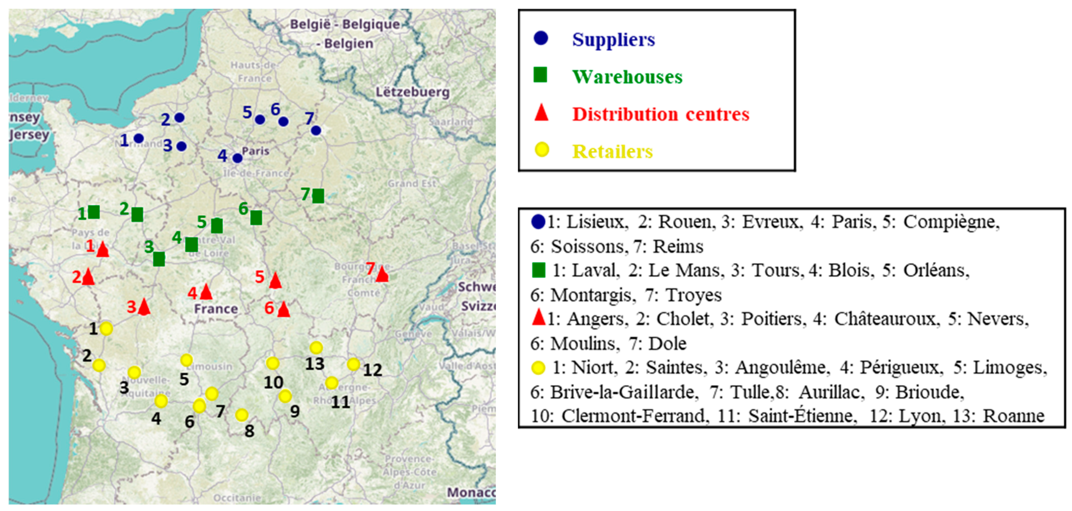
We apply our models to the distribution network represented in Figure 2. There are 34 nodes consisting of 7 suppliers delivering 7 food products to 13 retailers via shared warehouses and distribution centres for 6 weeks. The maximum number of warehouses and distribution centres to be opened is seven for each set. The number of hubs and their storage capacities are determined from the mathematical model.

The used distribution network is fictitious. The statistical data of CO₂ emissions and pallet characteristics are European. For this reason, we have chosen to treat a national distribution network located in France. There are two types of data: the first are extracted from statistical reports (unit emissions and warehouses’ unit opening costs); these data are described in [33,35,36,37], etc. The other data are hypothetical, such as unit transportation cost, customer demand, etc. The number of weeks allowed for late delivery for each partner is shown in

Table 3. Number of weeks allowed for late delivery.

Suppliers	i = 1	i = 2	i = 3	i = 4	i = 5	i = 6	i = 7
ap	1	0	0	1	0	2	1

. The rest of the data are represented in

Table 4. Other used data.

Parameters	Values	Data Sources
α	2
AP (m2)	0.96	Size of a European pallet (1.2 × 0.8)
$C{d}_t^p$ (€/Pallet)	5
$C{s}^p,C{l}^p,C{u}^p$ (€/Pallet)	1
$C{s}_m^p$ (€/Pallet)	10
$C{w}_m$ (€/m2)	400	[37,39]
$E{c}_m \left({\mathrm{kg}\mathrm{CO}}_2/{\mathrm{m}}^2\right)$	200	[33,40]
$E{o}_{m,t}\left({\mathrm{g}\mathrm{CO}}_2/\mathrm{kwh}\right)$	87.5	[33,40]
$W_{m,t}\left(\mathrm{kwh}\right)$	50
$S_m^p$ (Pallets)	0

. Similarly to the approach applied by [38], we use nominal demands ($W_{jt}^{pL}$) that follow a uniform distribution in the interval [0, 50]; these demands are given by Equation (144). The number of periods processed is equal to six (weeks), and each supplier has only one type of product. The used distances were calculated using Google Maps, and are shown in Appendix A.

$$W_{jt}^{pL}=rand\left(\left[0, 50\right]\right);\forall t \in T_1, j\in J,p\in P$$

(144)

We solved the resulting MILP formulations using IBM CPLEX 12.10 [41] on an Intel Core i7 with 2.40 GHz CPU and 6 GB of RAM, taking 5% of the uncertain parameters as the initial value of the uncertainty budget.

We used a heterogeneous fleet of vehicles to improve the vehicles fill rates, to select the appropriate vehicle capacity for each shipment, and to reduce the total distance travelled. According to [38], the employment of a heterogeneous fleet of vehicles can achieve an economy of scale and minimise the unit transportation costs. In this case study, we utilized three types of vehicles, with the data presented in

Table 5. The required data for the vehicles in use.

Parameters	Values			Data Sources
	v = 1	v = 2	v = 3
Qv (Pallets)	15	33	39	Benchmarking
Nmax	15	15	15
Payload (tons)	13	40	40
Cov (€/km)	0.3	0.5	0.7
Cqv (€/km)	0.5	1	1.2
Eov (g CO2/km)	511.2	772.68	772.68	[35]
Eqv (g CO2/km)	583.7	1096.09	1096.09	[35]
EMv (g CO2/km)	78	111	122	[36]

.

The results obtained in each uncertainty case and the fixed deterministic case (or worst case) are shown in

Table 6. Summary of the results obtained in the worst case and the robust cases.

Sustainability Indicators	Demands Uncertainty Case				Unit Transportation Costs Uncertainty Case
	Worst Case		Robust		Worst Case		Robust
	S_eco	S_env	S_eco	S_env	S_eco	S_env	S_eco	S_env
Transportation cost (EUR 106)	9.511	11.564	9.733	11.590	9.115	11.294	9.843	11.61
Storage cost (EUR 104)	1.942	5.615	0.663	6.701	0.408	6.815	0.561	6.961
Handling cost (EUR 105)	1.172	1.172	1.172	1.172	1.134	1.134	1.134	1.134
Opening cost (EUR 106)	4.804	4.396	4.829	4.828	4.262	4.265	4.807	4.804
Penalty cost (EUR 104)	3.736	4.132	6.951	7.558	4.004	3.912	5.777	6.203
Costs (EUR 107)	1.449	1.616	1.476	1.667	1.354	1.578	1.483	1.666
CO2 emissions due to vehicles (108 gCO2)	8.071	7.889	8.544	7.877	7.756	7.498	7.801	7.452
CO2 emissions due to hubs (109 gCO2)	2.198	2.198	2.415	2.414	2.132	2.133	2.404	2.402
CO2 emissions (109 g CO2)	3.005	2.987	3.269	3.202	2.907	2.883	3.184	3.147
	Maximum Number of Vehicles in Use in Uncertainty Case				Demands, Unit Transportation Costs and Maximum Number of Vehicles in Use in Uncertainty Case
	Worst Case		Robust		Worst Case		Robust
	S_eco	S_env	S_eco	S_env	S_eco	S_env	S_eco	S_env
Transportation cost (EUR 106)	9.114	11.294	9.114	11.140	9.900	11.752	10.407	11.299
Storage cost (EUR 104)	0.408	6.739	0.408	5.919	1.073	4.780	1.013	5.569
Handling cost (EUR 105)	1.134	1.134	1.134	1.134	1.723	1.172	1.172	1.172
Opening cost (EUR 106)	4.262	4.265	4.262	4.262	4.397	2.251	4.899	4.842
Penalty cost (EUR 104)	4.005	3.912	4.005	3.742	4.104	4.090	6.953	7.323
Costs (EUR 107)	1.353	1.560	1.353	1.561	1.446	1.638	1.551	1.639
CO2 emissions due to vehicles (108 gCO2)	7.758	7.498	7.758	7.529	8.589	8.032	8.035	8.685
CO2 emissions due to hubs (109 g CO2)	2.132	2.132	2.132	2.132	2.198	2.210	2.450	2.421
CO2 emissions (109 g CO2)	2.907	2.883	2.907	2.884	3.057	3.013	3.254	3.289

. The fixed deterministic case means that the used parameter values are those found in the worst case [20]. Therefore, the values of these parameters are equal to their nominal values plus the deviations provided by solving the robust model. S_eco represents the scenario dealing with the economic objective function, while S_env corresponds to that examining the environmental objective function.

4.1. The Impacts of Considering Uncertainty

To compare the results of the robust case with those of the worst case, we use a gap calculated as follows:

$$\mathrm{GAP}(\%)=\frac{Z_{S\_robust}-Z_{S\_ worst case}}{Z_{S\_worst case}} · 100$$

(145)

where $Z_{S\_ worst case}$ is the worst case optimal solution and $Z_{S\_robust}$ denotes the robust case.

The obtained results are shown in

Table 7. Reduction rates for the different studied cases (%).

Point of View	Robust	Worst Case
		Demands		Unit Transportation Costs		Maximum Number of Vehicles in Use		Demands, Unit Transportation Costs, and Maximum Number of Vehicles in Use
		S_eco	S_env	S_eco	S_env	S_eco	S_env	S_eco	S_env
Eco	S_eco	1.86%	-	9.53%	-	0.00%	-	6.77%	-
	S_env	-	3.16%	-	5.58%	-	0.06%	-	0.06%
Env	S_eco	8.79%	-	9.53%	-	0.00%	-	6.05%	-
	S_env	-	7.20%	-	9.16%	-	0.03%	-	9.16%

. We note that, when 5% of the demands take their worst case values, the total logistical cost of all scenarios is slightly higher in the robust approach than in the worst case. The robust economic scenario shows a total logistical cost and CO₂ emissions with increases of 1.86% and 8.79%, respectively, compared to the worst case. The robust environmental scenario also shows higher results, with 3.16% for the costs and 7.2% for the emissions, than the worst case. For the other levels of uncertainty, we always obtain gaps under 10%. When dealing with uncertain unit transport costs, the robust economic scenario shows a 9.53% increase from the worst case, for both costs and emissions. Furthermore, in the case of an uncertain maximum number of vehicles in use, the same finding is provided with gaps of 0% for the economic scenarios and 0.06% and 0.03% for the environmental ones. Finally, when all of the above-mentioned parameters are uncertain, there is an average increase of 6.85% while examining the costs and 7.80% for the minimisation of the CO₂ emissions, with maximum gaps of 7.26% and 9.16%, respectively. Despite the parameters’ disruptions, which generate additional costs and emissions, our robust model allows us to find optimal solutions with values close to the worst case ones. The proposed robust model is able to overcome the limits of the deterministic model, since it offers flexibility by taking into account the variation of the parameters without generating unmanageable costs and emissions. With this flexibility, real-life problems can be examined.

To further evaluate the impact of uncertainty, we use

Table 8. Capacities of upstream hubs (pallets).

Parameter	Approach	Scenario	Capacity (Pallets)
			m = 1	m = 2	m = 3	m = 4	m = 5	m = 6	m = 7
Demands	Robust	S_eco	0	0	435	0	916	1234	465
		S_env	0	0	0	0	1334	1694	0
	Worst case	S_eco	0	0	0	0	1163	1547	0
		S_env	0	0	475	723	426	771	413
Unit transportation costs	Robust	S_eco	0	0	0	0	1342	1698	0
		S_env	0	0	0	0	1334	1230	465
	Worst case	S_eco	0	0	0	0	1248	1497	0
		S_env	0	0	0	0	1211	1440	0
Maximum number of vehicles in use	Robust	S_eco	0	0	0	0	1252	1493	0
		S_env	0	451	452	0	1036	709	0
	Worst case	S_eco	0	0	0	0	1245	1499	0
		S_env	0	0	0	0	1211	1440	0
Demands, unit transportation costs, and maximum number of vehicles in use	Robust	S_eco	0	435	0	0	1397	1267	0
		S_env	0	435	0	421	771	1439	0
	Worst case	S_eco	0	464	0	0	1113	1242	0
		S_env	0	0	506	0	1458	860	0

,

Table 9. Capacities of downstream hubs (Pallets).

Parameter	Approach	Scenario	Capacity (Pallets)
			k = 1	k = 2	k = 3	k = 4	k = 5	k = 6	k = 7
Demands	Robust	S_eco	0	0	0	1720	1518	0	0
		S_env	0	0	733	1257	1269	0	0
	Worst case	S_eco	0	0	512	1133	1144	225	0
		S_env	0	0	915	902	570	781	0
Unit transportation costs	Robust	S_eco	0	0	0	1710	1509	0	0
		S_env	0	0	257	1460	1509	0	0
	Worst case	S_eco	0	0	0	1495	1086	223	0
		S_env	0	0	0	1575	1323	0	0
Maximum number of vehicles in use	Robust	S_eco	0	0	0	1507	1298	0	0
		S_env	250	0	450	1542	0	660	0
	Worst case	S_eco	0	0	0	1504	1302	0	0
		S_env	0	0	0	1575	1323	0	0
Demands, unit transportation costs, and maximum number of vehicles in use	Robust	S_eco	0	0	756	1016	986	523	0
		S_env	0	0	745	967	1015	511	0
	Worst case	S_eco	225	0	225	1342	890	224	0
		S_env	225	0	447	904	1145	210	0

and

Table 10. Number of vehicles in use.

Parameter	Approach	Scenario	Type 1	Type 2	Type 3	Total
Demands	Robust	S_eco	610	606	1310	2526
		S_env	509	522	1309	2340
	Worst case	S_eco	610	613	1320	2543
		S_env	516	548	1317	2381
Unit transportation costs	Robust	S_eco	581	562	1270	2413
		S_env	497	514	1270	2281
	Worst case	S_eco	583	564	1278	2425
		S_env	497	511	1262	2322
Maximum number of vehicles in use	Robust	S_eco	583	557	1278	2418
		S_env	500	532	1276	2308
	Worst case	S_eco	583	557	1278	2418
		S_env	497	511	1262	2270
Demands, unit transportation costs, and maximum number of vehicles in use	Robust	S_eco	604	624	1311	2539
		S_env	590	616	1309	2515
	Worst case	S_eco	609	632	1322	2563
		S_env	512	539	1308	2359

to compare the capacities of the hubs and the number of vehicles obtained in the robust and worst cases. When dealing with uncertain demands, the quantities of goods transported increase, improving the filling rate of vehicles, which means warehouses with bigger capacities. For this reason, the number of vehicles used in the robust case (2526 vehicles for S_eco and 2340 vehicles for S_env) is lower than that obtained in the worst case especially for the vehicles of type 3, which have the highest costs and emissions compared to the other vehicle types. Similarly, the capacities of the hubs are slightly higher in the robust case with uncertain unit transportation costs. However, when minimizing the costs, the robust approach presents a lower number of vehicles, which is reduced by the increase in the filling rate.

By comparing the results obtained in the maximum number of vehicles in use uncertainty case to those provided in the worst case, we note that when dealing with the economic scenario we have 2418 for both cases, compared to 2308 and 2270 vehicles in the environmental scenarios, constituting an increase of 1.67%. In the uncertainty case where all parameters are considered variable, the results show higher hub capacities due to variations in demand and unit transportation costs. However, since the transportation costs and demands impact the logistical costs directly, and the maximum number of vehicles in use reduces the total number of vehicles in use, the latter is lower in the robust economic scenario than in the worst case. We can conclude that uncertainty gives better or close results than the worst case, depending on the studied uncertain parameter.

4.2. Comparison of Economic and Environmental Scenarios’ Solutions

To compare the robust economic and environmental scenarios, the reduction rate is used. The obtained results are shown in

Table 11. Gaps obtained in the two scenarios.

		Demands		Unit Transportation Costs		Maximum Number of Vehicles in Use		Demands, Unit Transportation Costs, and Maximum Number of Vehicles in Use
		S_eco	S_env	S_eco	S_env	S_eco	S_env	S_eco	S_env
Eco	S_eco	-	−6.57%	-	−12.34%	-	−15.37%	-	−5.42%
	S_env	6.57%	-	12.34%	-	15.37%	-	5.42%	-
Env	S_eco	-	3.43%	-	1.16%	-	0.79%	-	−1.08%
	S_env	−3.55%	-	−1.18%	-	−0.80%	-	1.06%	-

, describing first the case of uncertain demands. Economically speaking, scenario S_eco is the best scenario, representing an improvement of 6.57% over S_env. However, for the preservation of the environment, scenario S_env is the most suitable, giving slightly better values (3.55%) than S_eco. For the cases of unit transportation costs, the maximum number of vehicles in use, and the combination of all uncertainty parameters, S_eco has the best economic results, while S_env is the best environmentally speaking.

Therefore, we can conclude that the economic scenario offers a good compromise between the obtained costs and CO₂ emissions; hence, it is the focus of the rest of this study.

4.3. The Impacts of the Uncertainty Level on the Network’s Optimal Configuration

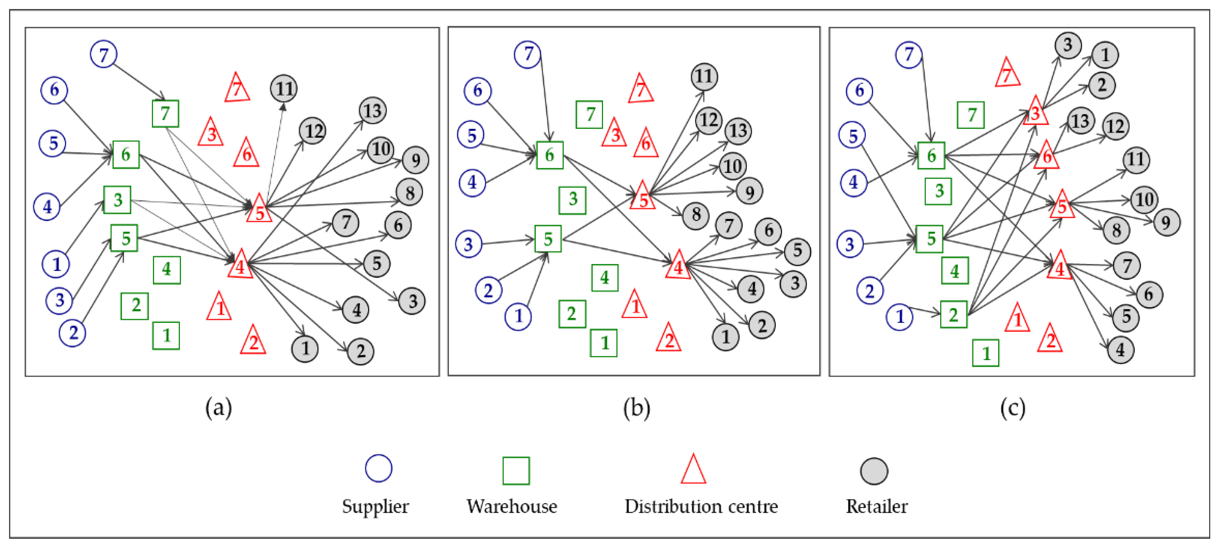
We study the impact of the uncertainty level on the optimal configuration of the distribution network, the total logistical cost, and the total CO₂ emission quantities. First, we present the optimal configurations obtained for the S_eco scenario illustrated in Figure 3. We note that the optimal configuration of the uncertain demand case is different from that of the unit transportation costs and number of vehicles in use cases, showing more open warehouses due to the use of more resources when increasing the demand. Obviously, by combining all of the uncertain parameters, the effect of demand uncertainty is highlighted, and the configuration has more open warehouses and distribution centres.

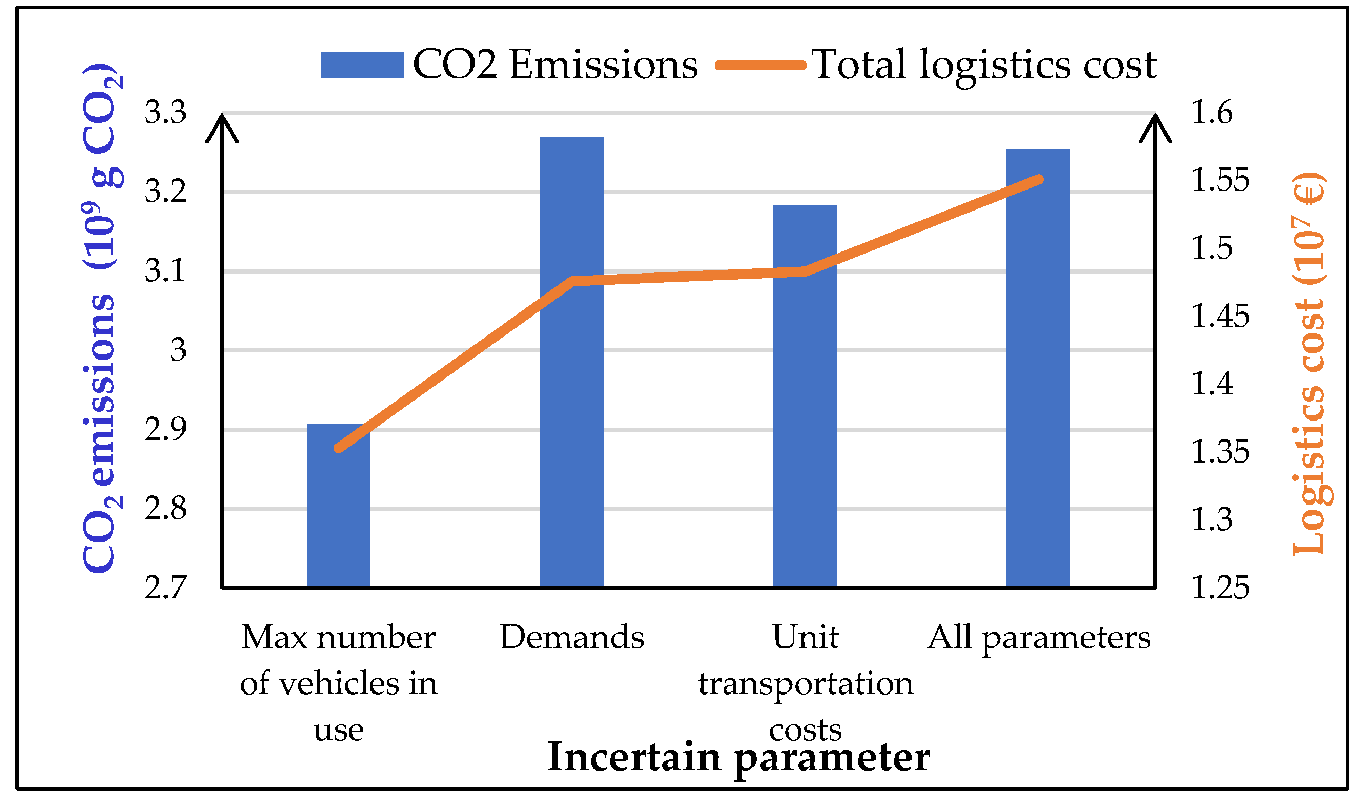
Figure 4 reveals the influence of each level of uncertainty on both the economic and environmental aspects. It is clear that the uncertainty of the unit transportation costs has the highest total logistical cost. Indeed, it increases when combined with the other levels of uncertainty. Therefore, from an economic point of view, the uncertainty of unit transportation costs has the most important influence on the total logistical cost. When dealing with the environmental aspect, the uncertainty of the maximum number of vehicles in use affects the CO₂ emissions slightly, because the decrease in this parameter’s value reduces the emissions. However, the increase in transportation costs enhances the filling rate of vehicles and, thus, increases the capacities of hubs, causing higher emissions. Moreover, when examining uncertain demands, there are more goods to deliver, which makes the total travelled distance longer, and causes an increase in the number of vehicles in use and the number of hubs; consequently, the CO₂ emissions will increase. When combining all of the uncertain parameters, the filling rate of vehicles increases and the number of vehicles decreases, compared to the uncertain demands case. For this reason, total emissions are lower than in the latter case.

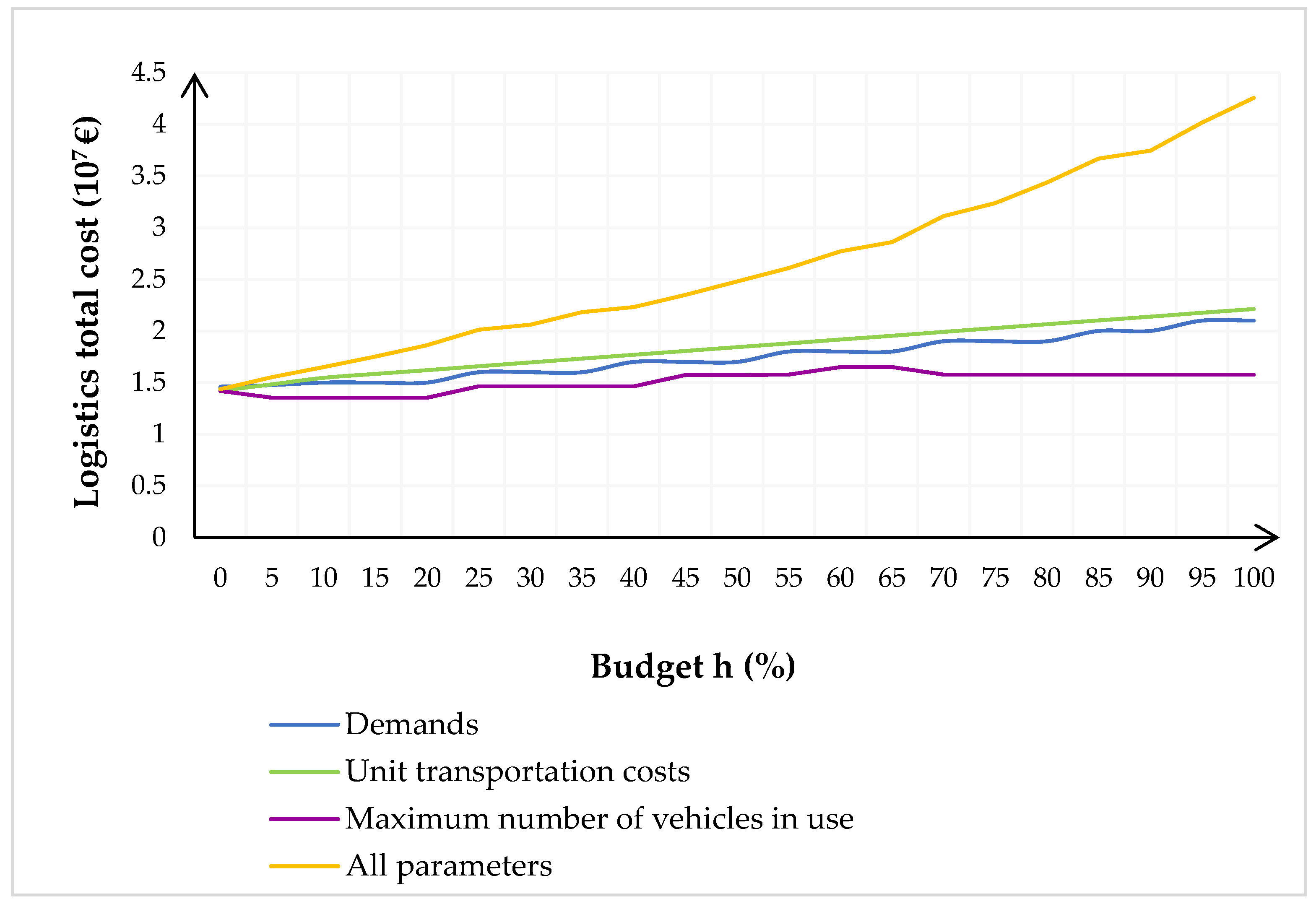
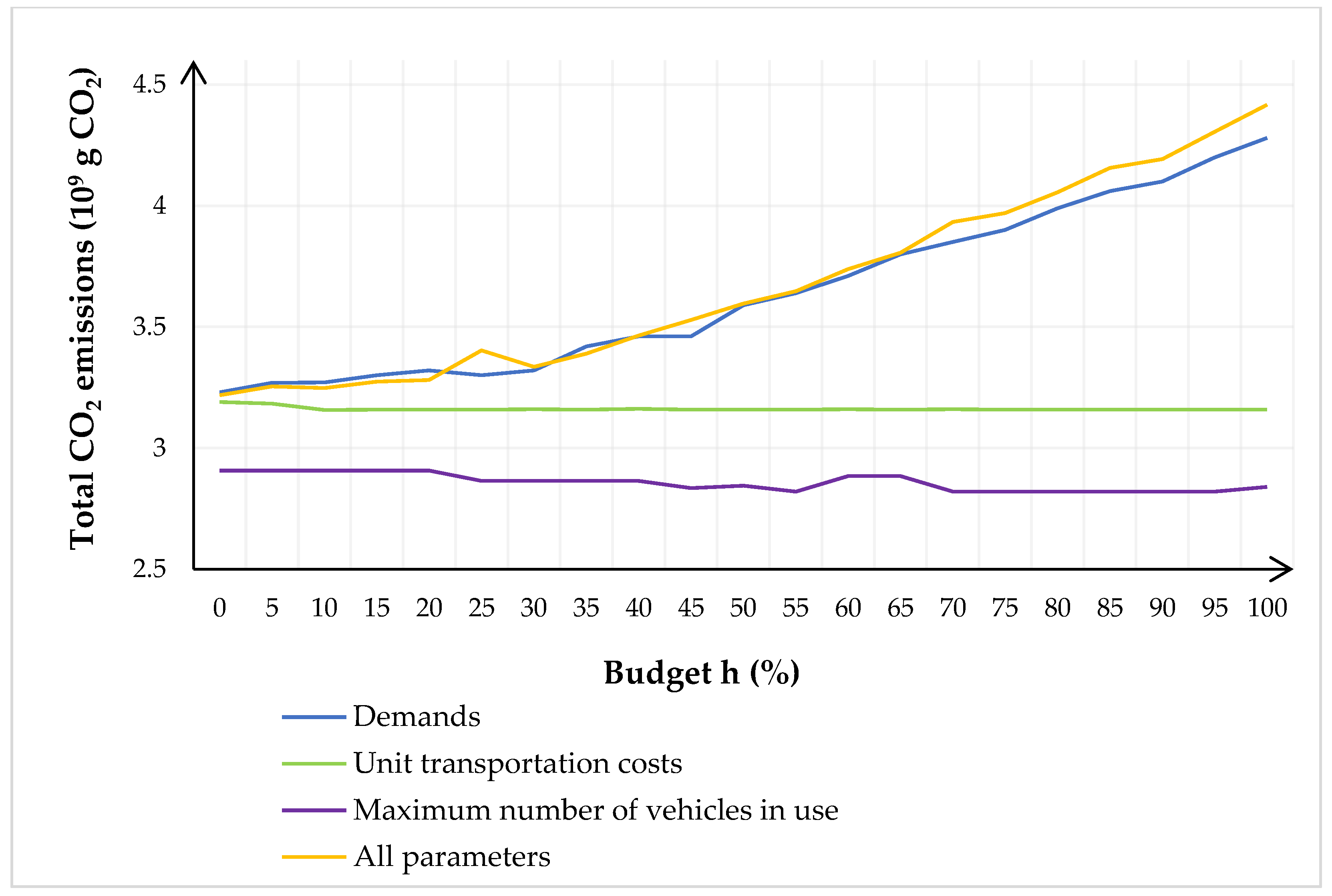
4.4. The Impacts of the Uncertainty Budget on Costs and CO₂ Emissions

Our modelling approaches allow decision-makers to select the level of robustness through uncertainty budgets. For some problems, it is unrealistic to assume that all parameter values change, and it is necessary to guard against this possibility [42]. In the following subsection, we will investigate the impacts of different uncertainty budgets on the total logistical cost and total CO₂ emissions; these effects are evaluated in Figure 5 and Figure 6, respectively. The curves in Figure 5 show that the total logistical cost for the cases of uncertain demand, unit transportation costs, and all of the parameters’ uncertainties increases with the uncertainty budget due to the selection of more uncertain demand parameters, unit transportation costs, and maximum number of vehicles in use. The uncertainty of all parameters is most sensitive to the increase in the budget. For the case of uncertainty in the maximum number of vehicles in use from the 70% value of the budget, the logistical cost becomes constant because of the uncertainty of all parameter budgets below 70%.

Figure 6 demonstrates the total CO₂ emissions as a function of the variation in the uncertainty budgets. With the increase in the latter, the number of parameters that can deviate from their nominal values increases; demand has the highest CO₂ emissions, as more resources are exploited. Beyond 70% and 10% of the budget, the emissions with a maximum number of vehicles in use or uncertain unit transportation costs become constant due to the choice of all of the parameters as variables at less than this value, the non-dependence of emissions on transportation costs, and the decrease in the number of vehicles in use. On the other hand, the increase in the uncertainty budgets of all uncertain parameters—namely, demands, unit transportation costs, and maximum number of vehicles in use—increases CO₂ emissions due to the considerable effect of demands on them.

5. Conclusions

In this study, we addressed the problem of designing a collaborative distribution network under uncertainty. Our objective was to minimise the logistical costs and CO₂ emissions. Four uncertain models were proposed, examining demands, unit transportation costs, and maximum number of vehicles in use as uncertain parameters, both jointly and separately. We considered an interval of uncertainty for demands, unit transportation costs, and maximum number of vehicles in use, and used an uncertainty budget to control the level of conservatism in solution networks. We introduced mixed-integer linear programming formulations for each of the considered robust counterparts. To validate our models, we solved them with a commercial solver using a case study. Then, we analysed the obtained results by discussing the impact of uncertainty, the effects of the levels of uncertainty from an economic and environmental point of view, and the effects of the variation in the uncertainty budget, whose increase allowed the choice of more parameters deviating from their nominal values. We noticed that, for the economic and environmental scenarios, uncertainty made it possible to obtain results close to the worst case. Indeed, despite the variation in the data, the robust approach presents better or close results while dealing with the number of vehicles in use, depending on the uncertain parameter analysed. Comparing the considered scenarios according to their objectives, we noticed that the economic scenario offered a good compromise between the obtained values of costs and CO₂ emissions. It was also obvious that the optimal configuration of the uncertain demands case had more open warehouses. When dealing with the influence of the uncertainty levels, the unit transport costs had the most important impact from the economic point of view, unlike the environmental case, where the influence of the demands was the most dominant. The studied problem in this paper is NP-hard; thus, as the size of the problem increases, the use of a commercial solver can be considered as a factor leading to long computation times. Heuristic methods such as genetic algorithms seem to be a promising approach to cover large instances. Moreover, simultaneously minimising the logistical costs and the CO₂ emissions would be preferable to ensure sustainability.

References

- Ayadi, H.; Hamani, N.; Kermad, L.; Benaissa, M. Novel Fuzzy Composite Indicators for Locating a Logistics Platform under Sustainability Perspectives. Sustainability 2021, 13, 3891. [Google Scholar] [CrossRef]
- Pan, S.; Trentesaux, D.; Ballot, E.; Huang, G.Q. Horizontal Collaborative Transport: Survey of Solutions and Practical Implementation Issues. Int. J. Prod. Res. 2019, 57, 5340–5361. [Google Scholar] [CrossRef] [Green Version]
- Mrabti, N.; Hamani, N.; Delahoche, L. A Sustainable Collaborative Approach to the Distribution Network Design Problem with CO2 Emissions Allocation. Int. J. Shipp. Transp. Logist. 2020. [Google Scholar] [CrossRef]
- Aloui, A.; Hamani, N.; Derrouiche, R.; Delahoche, L. Systematic Literature Review on Collaborative Sustainable Transportation: Overview, Analysis and Perspectives. Transp. Res. Interdiscip. Perspect. 2021, 9, 100291. [Google Scholar] [CrossRef]
- Ouhader, H.; Kyal, M.E. Assessing the Economic and Environmental Benefits of Horizontal Cooperation in Delivery: Performance and Scenario Analysis. Uncertain Supply Chain Manag. 2020, 303–320. [Google Scholar] [CrossRef]
- Mrabti, N.; Gargouri, M.A.; Hamani, N.; Kermad, L. Towards a Sustainable Collaborative Distribution Network 4.0 with Blockchain Involvement. In Proceedings of the 22nd IFIP Pro-VE 2021 on Smart and Sustainable Collaborative Networks 4.0, Saint Etienne, France, 22–24 November 2021. [Google Scholar]
- Zetina, C.A.; Contreras, I.; Cordeau, J.-F.; Nikbakhsh, E. Robust Uncapacitated Hub Location. Transp. Res. Part B Methodol. 2017, 106, 393–410. [Google Scholar] [CrossRef]
- Fischetti, M.; Monaci, M. Light Robustness. In Robust and Online Large-Scale Optimization; Springer: Berlin/Heidelberg, Germany, 2009; Volume 5868, pp. 61–84. ISBN 978-3-642-05464-8. [Google Scholar]
- Ben-Ayed, O. Parcel Distribution Network Design Problem. Oper. Res. 2013, 13, 211–232. [Google Scholar] [CrossRef]
- Hu, L.; Zhu, J.X.; Wang, Y.; Lee, L.H. Joint Design of Fleet Size, Hub Locations, and Hub Capacities for Third-Party Logistics Networks with Road Congestion Constraints. Transp. Res. Part E Logist. Transp. Rev. 2018, 118, 568–588. [Google Scholar] [CrossRef]
- Habibi, M.K.K.; Allaoui, H.; Goncalves, G. Collaborative Hub Location Problem under Cost Uncertainty. Comput. Ind. Eng. 2018, 124, 393–410. [Google Scholar] [CrossRef]
- Contreras, I.; Cordeau, J.-F.; Laporte, G. Stochastic Uncapacitated Hub Location. Eur. J. Oper. Res. 2011, 212, 518–528. [Google Scholar] [CrossRef]
- Adibi, A.; Razmi, J. 2-Stage Stochastic Programming Approach for Hub Location Problem under Uncertainty: A Case Study of Air Network of Iran. J. Air Transp. Manag. 2015, 47, 172–178. [Google Scholar] [CrossRef]
- Habibzadeh Boukani, F.; Farhang Moghaddam, B.; Pishvaee, M.S. Robust Optimization Approach to Capacitated Single and Multiple Allocation Hub Location Problems. Comput. Appl. Math. 2016, 35, 45–60. [Google Scholar] [CrossRef]
- Meraklı, M.; Yaman, H. Robust Intermodal Hub Location under Polyhedral Demand Uncertainty. Transp. Res. Part B Methodol. 2016, 86, 66–85. [Google Scholar] [CrossRef] [Green Version]
- Kazemian, I.; Aref, S. Hub Location under Uncertainty: A Minimax Regret Model for the Capacitated Problem with Multiple Allocations. Int. J. Supply Chain Inventory Manag. 2017, 2. [Google Scholar] [CrossRef]
- Alumur, S.A.; Nickel, S.; Saldanha-da-Gama, F. Hub Location under Uncertainty. Transp. Res. Part B Methodol. 2012, 46, 529–543. [Google Scholar] [CrossRef]
- Talbi, E.-G.; Todosijević, R. The Robust Uncapacitated Multiple Allocation p -Hub Median Problem. Comput. Ind. Eng. 2017, 110, 322–332. [Google Scholar] [CrossRef]
- Bertsimas, D.; Sim, M. Robust Discrete Optimization and Network Flows. Math. Program. 2003, 98, 49–71. [Google Scholar] [CrossRef]
- Correia, I.; Nickel, S.; Saldanha-da-Gama, F. A Stochastic Multi-Period Capacitated Multiple Allocation Hub Location Problem: Formulation and Inequalities. Omega 2018, 74, 122–134. [Google Scholar] [CrossRef]
- Martins de Sá, E.; Morabito, R.; de Camargo, R.S. Benders Decomposition Applied to a Robust Multiple Allocation Incomplete Hub Location Problem. Comput. Oper. Res. 2018, 89, 31–50. [Google Scholar] [CrossRef]
- Ghaffarinasab, N. An Efficient Matheuristic for the Robust Multiple Allocation P-Hub Median Problem under Polyhedral Demand Uncertainty. Comput. Oper. Res. 2018, 97, 31–47. [Google Scholar] [CrossRef]
- Rahmati, R.; Bashiri, M. Robust Hub Location Problem with Uncertain Inter Hub Flow Discount Factor. In Proceedings of the International Conference on Industrial Engineering and Operations Management, Paris, France, 26–27 July 2018; p. 10. [Google Scholar]
- Lozkins, A.; Krasilnikov, M.; Bure, V. Robust Uncapacitated Multiple Allocation Hub Location Problem under Demand Uncertainty: Minimization of Cost Deviations. J. Ind. Eng. Int. 2019, 15, 199–207. [Google Scholar] [CrossRef] [Green Version]
- Peiró, J.; Corberán, Á.; Martí, R.; Saldanha-da-Gama, F. Heuristic Solutions for a Class of Stochastic Uncapacitated P-Hub Median Problems. Transp. Sci. 2019, 53, 1126–1149. [Google Scholar] [CrossRef]
- Ben Mohamed, I.; Klibi, W.; Vanderbeck, F. Designing a Two-Echelon Distribution Network under Demand Uncertainty. Eur. J. Oper. Res. 2020, 280, 102–123. [Google Scholar] [CrossRef]
- Shang, X.; Yang, K.; Jia, B.; Gao, Z. The Stochastic Multi-Modal Hub Location Problem with Direct Link Strategy and Multiple Capacity Levels for Cargo Delivery Systems. Transp. Transp. Sci. 2020, 17, 380–410. [Google Scholar] [CrossRef]
- Li, S.; Fang, C.; Wu, Y. Robust Hub Location Problem With Flow-Based Set-Up Cost. IEEE Access 2020, 8, 66178–66188. [Google Scholar] [CrossRef]
- Rahmati, R.; Neghabi, H. Adjustable Robust Balanced Hub Location Problem with Uncertain Transportation Cost. Comput. Appl. Math. 2021, 40, 14. [Google Scholar] [CrossRef]
- Jeyakumar, V.; Rubinov, A.M. (Eds.) Continuous Optimization: Current Trends and Modern Applications. In Applied Optimization; Springer: New York, NY, USA, 2005; ISBN 978-0-387-26769-2. [Google Scholar]
- Ben-Tal, A.; El Ghaoui, L.; Nemirovskij, A.S. Robust Optimization; Princeton Series in Applied Mathematics; Princeton University Press: Princeton, UK, 2009; ISBN 978-0-691-14368-2. [Google Scholar]
- Mrabti, N.; Hamani, N.; Delahoche, L. The Pooling of Sustainable Freight Transport. J. Oper. Res. Soc. 2020, 1–16. [Google Scholar] [CrossRef]
- ADEME (Agence De l’Environnement et de la Maîtrise de l’Energie). Calcul des Facteurs d’Émissions et Sources Bibliographiques Utilisées. Methode Bilan Carbone; ADEME: Angers, France, 2010. [Google Scholar]
- Hamaz, I. Méthodes d’Optimisation Robuste pour les Problèmes d’Ordonnancement Cyclique; Université Paul Sabatier: Toulouse, France, 2018. [Google Scholar]
- Hickman, J.; Hassel, D.; Joumard, R.; Samaras, Z.; Sorenson, S. Methodology for Calculating Transport Emissions and Energy Consumption. Int. J. Cult. Tour. Hosp. Res. 1999, 11, 67–80. [Google Scholar]
- OEET (Observatory Energy Environment of Transport). Available online: https://www.bilans-ges.ademe.fr/documentation/UPLOAD_DOC_FR/index.htm?transport_routier_de_marchandi%20.html (accessed on 3 April 2021).
- Le Véritable Cout de Construction d’un Entrepôt Logistique et Industriel-20/20. Available online: https://www.rachatducredit.com/credit-bail-avec-bail-a-construction-543769.html (accessed on 13 August 2021).
- Serper, E.Z.; Alumur, S.A. The Design of Capacitated Intermodal Hub Networks with Different Vehicle Types. Transp. Res. Part B Methodol. 2016, 86, 51–65. [Google Scholar] [CrossRef]
- Guide des Prix de la Construction d’Entrepôt ou de Local Industriel. Available online: https://travaux.mondevis.com/construction-entrepot/guide/ (accessed on 28 August 2021).
- Ayadi, A. Vers Une Organisation Globale Durable de l’approvisionnement Des Ménages: Bilans Économiques et Environnementaux de Différentes Chaînes de Distribution Classiques et Émergentes Depuis l’entrepôt Du Fournisseur Jusqu’au Domicile Du Ménage. Ph.D. Thesis, Université Lumière Lyon, Lyon, France, 2014. [Google Scholar]
- CPLEX. IBM ILOG.12.10: User’s Manual for CPLEX; International Business Machines Corporation: Incline Village, NV, USA, 2019. [Google Scholar]
- Snoussi, I.; Hamani, N.; Mrabti, N.; Kermad, L. Robust Optimization for Collaborative Distribution Network Design Problem. In Proceedings of the 22nd IFIP Pro-VE 2021 on Smart and Sustainable Collaborative Networks 4.0, Saint Etienne, France, 22–24 November 2021. [Google Scholar]
Figure 1.
Example of a distribution network.
Figure 2.
The examined distribution network.
Figure 3.
Optimal network configurations of the scenario S_eco: (a) distribution network in the demand uncertainty case; (b) distribution network in the unit transportation costs and number of vehicles in use uncertainty cases; (c) distribution network in the combined parameters uncertainty case.
Figure 4.
Impacts of different levels of uncertainty on costs and CO2 emissions.
Figure 5.
Impacts of the uncertainty budget on the total logistical cost (EUR 107).
Figure 6.
Impacts of the uncertainty budget on the CO2 total emissions (109 g CO2).