GDP and Public Expenditure in Education, Health, and Defense. Empirical Research for Greece

Abstract

Wagner Law and Keynesian approaches are the two fundamental theories of public finance. The aim of this study is to assess empirical evidence for the public spending–national income relationship at a disaggregated level for the time period 1995–2019. The sectoral public expenditures include education, health, and defense. The data employed were derived by EUROSTAT and OECD. Based on our findings, a sole relationship of the variables was validated, while the causality of the relationship provides conflict results depending on whether two-variate or multivariate methodology is employed. In the case of the multivariate framework that outperforms the two-variate approach in terms of information, the causality is directed from government expenses to the GDP level, validating the Keynesian approach in the long run as well as in the short run. On the other hand, the results validate Wagner Law based on the results of Granger causality pairwise test. A potential interpreatation for the results found is related to the measures imposed by the Memorandum, since the disproportionate cuts of the public expenses in the period of crisis have determined the evolution of national income. The scientific value of the presents study stands on the suggestion of potential effective measures aiming at the limitation of national income shrinkage in periods of severe economic crises worldwide.

1. Introduction

Greece over the last decade has experienced a severe economic crisis. Compared to the year 2009, the starting point of the economic crisis, in the year 2013, more than a quarter of the country’s output had been lost. In addition, all the macroeconomic figures are indicative of a multifaceted economic problem that is difficult to handle. For instance, the unemployment rate was approaching 27% and the national debt surpassed 110% in the same year. This economic disaster, as expected, was also accompanied by severe consequences for the total society. In subtle, more than 900,000 people in only three years were found at risk of poverty or social exclusion in a population of around 11 million [1].

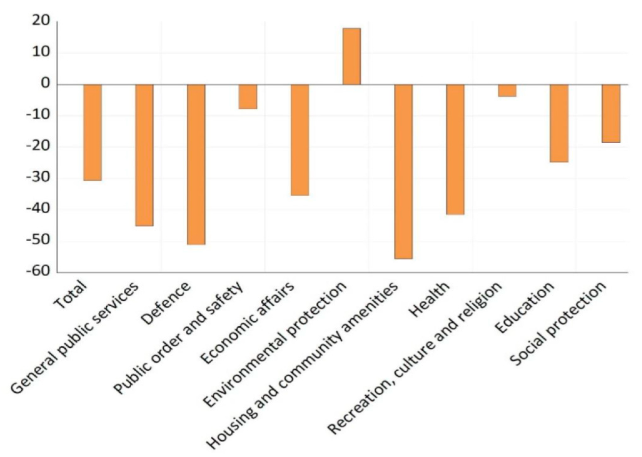
The extension of the Memorandum in valid since the year 2010 has imposed several restrictions on public expenditure. This fact, along with a sharp decrease in GDP, has attracted scientific interest for studying their relationship. The present work aims to study the validity of the public expenditure–national income relationship with the econometric tools of causality and cointegration. The model presented is a result of research on the financing of education in Greece and the relationship between the expenditures of the Welfare State and GDP. The change in the public expenditure per function is illustrated in Figure 1:

The causal relationship between the public sector expenditures and economic development for an economy may be adequately interpreted either with the Keynesian or the Wagner law approach. According to the Keynes approach, public expenditure contributes to the growth of national income in the short run with the mechanism of multipliers. On the other hand, Wagner argued that an increasing national income (namely economic growth) leads to an increase in public expenditures. The theory described above is known as Wagner’s Law. To synopsize causality from public expenditure to national income reflects the validity of the Keynesian approach, while the vice-versa causality is synopsized in Wagner’s law [2].

Another significant aspect of the particular issue is related to the nature of productivity for public expenditure. Implicitly, public expenditure may be categorized into productive and unproductive in terms of consumption and investment headings, based on previous research. For instance, public spending in the health and education sector is considered productive since more schooling and better health in individuals (as a result of a better-financed educational and health system) results in higher individual earnings and therefore higher GDP (Keynesian approach) [3]. The expenditure on education is one of the major tools promoting economic growth due to its ability to enhance human capabilities and realize social and economic development, while it functions as a means to poverty alleviation and contributing to political awareness and stability [4].

Furthermore, the development of human capital in a way that enables training, health improvement, migration, and other investments that allow an individual’s productivity enhancement is a result of promoting all stages of education [5].

One of the most significant works on the mechanisms of economic growth is provided by Lucas [6], which studies optimality in the allocation of the economic agents’ time dedicated to education (human capital accumulation) and production. The problem confronted by an individual in Lucas’s model concerns the balance achieved between physical capital and human capital. In another work based on the partial equilibrium version of the Lucas model in the form of a two-stage optimization problem in which the time devoted to work versus time devoted to human capital accumulation decision and its relation to consumption can be handled separately. In the first stage, agents optimally choose the division of time between human capital accumulation and production to maximize lifetime income, while in the second stage agents distribute consumption optimally over their infinite lives, given their lifetime income [7].

As far as public health is concerned, this is also a significant component of human capital. An increase in health expenditure and improvements in the field of health enhances the quality of human capital. There are numerous theoretical and empirical studies indicating that an increase in human capital affects economic growth positively [8].

The role of economic growth in the long term with public expenditure on health is also a common finding for the studies [8]. Furthermore, in times of economic crisis, different studies tried to identify its consequences on public health, and not vice versa. It is common practice during an austerity period for sharp decreases in health expenditure to take place [9].

This can be attributed to the easy application of health expenditure decreases, especially in the case of Greece, where within the first five years of the economic crisis, the public expenditure for health was halved [1].

Last but not least, the level of military spending is influenced by many international factors and events, including, among others, exogenous real or perceived threats, armed conflicts or military alliances, and policies aiming to maintain peace mainly for domestic reasons. The decision for defense spending is a government’s authority within the allocation process of public spending among competing objectives [10].

It should be stressed that military spending may affect a country’s economic growth via a variety of channels even though it is considered a non-productive expenditure with limited contribution to a fruitful and productive socio-economic life for its citizens [10].

In most cases, the studies focus on the public expenditure–national income relationship as a total amount, while on the other hand, in some cases, the studies involve disaggregated data on sectoral public expenditures including health, education, and defense, or others employed in the econometric analysis. The significance of this relationship is even higher in the case of an economic crisis. Explicitly, in periods of recession the central authorities’ abilities are limited to balance their economy via fiscal measures. This is achievable only in the case of the share of government spending to GNP is increasing [11].

The present analysis involves the study of the national income–sectoral public expenditure relationship, namely expenditures for education, defense, and health, for a period within which Greece was going through a severe crisis within a Framework determined by Memorandum that is restrictive to measures taken for expanding the public expenditure and, in sequence, to economic growth. Therefore, studying the particular relationship may be vital for policymaking to shrink austerity through economic growth and at the same time to secure satisfactory socio-economic conditions for the citizens in Greece, since health and education are more than requirements for an economy’s economic growth.

2. Literature Review

Various studies, especially in recent decades, are focusing on the causality relationship between GDP and different types of government expenditures, with conflicting results in the majority of them. The public expenses of each country on education, health, and defense are related to a number of different factors, including economic growth, political conditions, and corruption [3,4,5,6,7,8,9,10].

A basic study examining defense spending is Baran and Sweezy’s work [12] which adopts Marxist analytical tools to understand how defense is important in order to maintain capitalism. On the other hand, we have to admit that defense expenses from every nation are difficult to know because they are confidential.

Castles [13], aiming to explain different ways of processing education expenditure among OECD member countries, formed a five-factor model consisting of school enrolment rates, demographic pressure, economic growth, the political functioning system, and cultural influence of the dominant religion. Through a multifactorial analysis, he concluded that educational expenditure is multidimensional. Each of the factors studied seems to have a different impact in different OECD countries. All factors occupy between one-quarter and one-half of the range of spending on education, although per capita change in GDP (economic growth) has, to some extent, the greatest impact on education expenditure.

In a relevant study, [14] investigates whether different types of Welfare States have different impacts on social policy outcomes. Their study is based on Esping-Andersen’s work [15], who identified three different systems of the Welfare State in advanced industrial societies: liberal, conservative, and social democratic. Each of the three systems of the Welfare State is distinctly structured in terms of organizational logic, social stratification and social inclusion and formulates its own priorities in terms of health, unemployment, and old-age and pension insurance. The three systems of Welfare States are examined in conjunction with Castles’s research in order for a relation of the variation of education expenditure to a specific system of the Welfare State to be identified. Finally, it is investigated whether, as Heidenheimer [16] suggests, “there is evidence of a trade-off between education and other social security policies as alternative Welfare State strategies”. A relationship between distinct educational policies and types of Welfare States has been verified.

Liberal states seem to spend a larger proportion of total public expenditure on education compared to conservative and social democratic ones. Social democratic states follow the liberal ones in public spending on education. However, they afford the largest share of GDP to education, while conservative states are ranked last in public spending on education. At the same time, Hega and Hokenmaier [17] confirm that education, as a tool of public policy, is used as a countervailing factor in relation to other welfare strategies.

Empirical research has also shown that a high proportion of public spending on social and educational policies is directed in relation to the ‘demand’ factors, mainly the demographic structure of each country [18], while the age composition of societies is a determining factor in the distribution of social welfare resources [19].

More specifically, research in the fields of political science and sociology, focusing on parameters of public policymaking and funding, shows that in some cases social and educational policies are closely related to target age groups. In relevance to Esping-Andersen’s typology, Social Democratic States seem to be characterized by a balance of social spending across the younger and the elderly generations. Contrarily, both conservative and liberal states implement policies that are preferentially targeted at limited age ranges, either the younger generations (the Netherlands, Ireland, Australia) or the elderly ones (Italy, Austria, Greece, Japan, USA). What is also noteworthy is a distinction between OECD members in countries where political life is dominated by clientelism and patronage of political parties (Austria, Italy, Greece, Spain, USA) and those with dominant programmatic political parties (Northwest Europe, Canada, Australia, New Zealand). This is a distinction that seems to identify another crucial variable regarding the allocation of public funds and a positive discrimination in favor of specific age groups [20].

Focusing on another variable, that of corruption, Mauro [21] demonstrates a correlation of government spending on education with the levels of corruption characterizing the states. According to his study, high levels of corruption lead to limited government funding on education, as the education sector is an unattractive field for rent-seeking.

Castells [22] argues that education is a significant tool for economic development directly and indirectly through other fields. To be more specific, in the case that people are educated, they invest in self-improvement, and at the same time help the economy grow and thrive. Nowadays, higher education makes people capable of being active members socially and economically [23]. In Algeria, Saudi Arabia, and Jordan, a study by Boudia and Bens Zidane [24] proved the positive role of investment in higher education and GDP. In contrast to the above, Psaharopoulos and Patinos [22] believe that primary education is the most important investment for a society, compared to higher education.

However, it is not acceptable to ignore a lot of studies which show that expenditure on education is connected with GDP and economic growth. A study which took place in Algeria [23] proved that between the years of 1968 and 2007, education and economic growth were connected, and so education is important to be funded by the government. Additionally, a study [24] confirmed that spending on education contributes to improving the social and economic status of the countries.

Through the years, numerous studies have examined the relationship between social expenditure and economic growth (evolution of GDP). Economic growth is usually accompanied by political instability, which also enhances social expenditure [25]. Kharasgani’s [26] study showed that economic growth depends on education, wellbeing, and life expectancy as well. The same answer has been given by other studies [27,28]. To be more specific, [28] confirms the special role of education on raising the productivity, energy, and creativity of people.

Expenditure on health, education, and defense is also the focal point of a lot of studies [29,30], while some of them [31,32] study their association with GDP and economic growth. Based on the findings of some studies [33,34], the trade-off between defense and health is negative, while on the other hand, it is positive between defense and education. In another study, Sheetz [35] found that defense expenditure increases with higher speed than education and health in Latin America. A significant result of the aforementioned studies concerns the competitive use of public expenditure among health and education. More specifically, an increase in health expenditure entails a decrease in education expenditure, and vice versa.

As for the Keynesian or Wagner law approaches being studied, numerous works can be mentioned [3,4,5,6,7,8,9,10,36]. Apart from the findings validating either the Keynesian school or the Wagnerian school, there are cases where both GE and economic growth have caused each other a result that validates the bi-directional relationship for the variables to be studied [37,38]. More specifically, for developing countries, in most cases the public expenditures do have an impact, either positive or negative, on national income [39,40,41,42]. In the case of the European Union, Afonso and Alves [43] found for Austria, France, the Netherlands, and Portugal that an increase in national income enhances government spending (validity of the Wagner law), though the starting point of economic crisis, as well as the severe interference of the EU on fiscal and monetary policy, has coincided with the imposition of specific public spending on education, health, and defense. For Greece, an effort was made to examine the validity of the Wagner Law with the econometric tool of cointegration for the data of over a century, covering a time period of 1833–1938 and validating the Wagner Law, a result that is in line with other studies on different economies but at an early stage of development [44,45]. In addition, [44] argues that Wagner’s hypothesis validation in periods of economic crises is justified by the need for the restructuring of the State in order to overcome the dominance of the recessional conditions.

The present study makes an effort to unveil the valid theory for the economy under review that is developed, and yet under a severe economic crisis. The analysis involves disaggregated data for public expenses, including education, defense, and health. Thus, the novelty of the present work is twofold. First of all, the Wagner law is examined for the disaggregated data of public expenses, with the assistance of structural breaks enabling the detection of changes in the economic policy adopted, and secondly, this is the first time that, for the case of Greece, both theoretical frameworks are examined for a time period in which specific economic conditions dominate (severe economic crisis and Momerandum). Thus, our findings may be of great value for policy makers in order to successfully tackle public management.

3. Research Methodology

The relationship among the variables that subtly describes the evolution of GDP and shares for the most significant sectors, namely health, education, and defense, was examined with the application of the Johansen cointegration technique. All the data are in logarithmic form, they are annual, and the period studied extends from 1995–2019. Prior to the implementation of the aforementioned methodology, we had to validate whether the time series are integrated of first order (I(1)). This means that the time series studied are non-stationary in the levels and stationary in the first differences. The first-order integration is a necessary condition being fulfilled by the variables for the implementation of the Johansen cointegration technique. The stationarity condition for the time series mentioned above was examined with the assistance of break unit root tests that may well capture potential structural breaks in their evolution. This is a necessary procedure in applied research aiming to identify differences between trend and difference stationary data. Explicitly, the conventional unit root tests in comparison with the break unit root tests are biased toward a false unit root, null when the data are trend stationary with a structural break [45].

Having concluded that the time series examined are either I(1) or I(0), their combination can be tested for stationarity with the application of the Johansen cointegration technique; thus, we can use the Johansen technique to examine whether there is a combination (linear relation) of the variables that is stationary. In this case, the variables studied are cointegrated and hence, there is a long-run relationship between them.

The Johansen cointegration technique [46], with two likelihood ratio (LR) test statistics—namely, the trace and the maximal eigenvalue (A-max) statistics—identifies the number of cointegrating vectors in non-stationary time series. One cointegrating equation validates the cointegration and, in sequence, a sole long-run relationship among the variables employed. The results are based on critical values from Osterwald-Lenum [47], which differ slightly from those reported in Johansen and Juselius [46]. In our case, we used an extra exogenous dummy variable corresponding to the year 2009 in order to capture the impacts of the economic crisis on all aspects of life in Greece.

The next step involved the Error Correction Model estimation. This process is based on the Granger representation theorem, according to which, if a cointegrating relationship exists among a set of I(1) series, a dynamic error-correction (EC) representation of the data also exists [48].

The Vector Error Correction Model estimation serves as a means of examination for the direction of the causality between the variables employed. The statistical significance of the cointegrating equation coefficient determines the causality direction, while it captures not only the long-term, but also the short-term dynamics of the model.

Two different methodologies explicitly followed the impulse response and variance decomposition analysis. The particular tests efficiently describe the evolution of the shock through the VECM system under review [49].

The impulse response analysis identifies the dynamics among the variables and explicitly estimates the response of a studied variable to a unit change, attributed to a shock or innovation in the value of one of the errors of the variables participating in VECM. More specifically, the generalized impulse response [49] in our study is a tool that describes the dynamics of a time-series model by mapping out the reaction in the public expenses for health, for instance, to a one-standard-deviation shock to the residual in the GDP or the expenses for health or defense.

Under the condition that no error is verified for each of the variables of the system, the whole system would return to zero in future periods. Moreover, if the system presented by Equation (1) is considered with a time lag (t − i), the methodology under review identifies the responsiveness of the endogenous variables in case a unit shock or impulse is observed in the errors of the model variables under review.

The model we present is a result of research on the financing of education in Greece and the relationship between the expenditures of the Welfare State and GDP.

The VAR process we employed is provided by Equation (1):

$$x_t=\Phi D_t+{\displaystyle \sum _{i=1}^k{\Pi }_i{x}_{t-i}+{\epsilon }_t\hspace{1em}\hspace{1em}t=1,2,\dots ,T\hspace{1em}\hspace{1em}}$$

(1)

The particular process described by x_t, the vector of GDP and public expenses for health, education, and defense, is covariance stationary, integrated of order d, while the error term ε_t is p dimensional and assumed to be i.i.d. (identically, independently distributed) with zero mean and a positive definite covariance matrix Ω.

The h-ahead forecast error for the x_t process is Equation (2):

$$x_{t+h}-E[x_{t+h}/I]={\displaystyle \sum _{j=0}^{h-1}{C}_j{\epsilon }_{t+h-j}}$$

(2)

where I is an information set which includes the previous values of x_s until period t, as well as the entire time path for D_t. The p × p matrices Cj are given by C₀ = I_p and

$$C_j={\displaystyle \sum _{i=1}^{\min k,j}{\Pi }_i{C}_{j-i}\hspace{1em}\hspace{1em}j\ge 1}$$

(3)

so that all C_j matrices can be estimated from the Π_i matrices.

The generalized impulse-response function was introduced by Koop, Pesaran, and Potter [33], as synopsized in Equation (4):

$$G{I}_x\left(h,\hspace{0.17em}\delta ,\hspace{0.17em}{I}_{t-1}\right)=E\left[x_{t+h}/{\epsilon }_t=\delta ,\hspace{0.17em}{I}_{t-1}\right]-E\left[x_{t+h}/I_{t-1}\right]$$

(4)

where δ is a known vector. In the VAR process, the equation takes the following form:

$$G{I}_x\left(h, \delta ,\hspace{0.17em}{I}_{t-1}\right)=G_h\delta$$

(5)

The selection of δ is a critical issue for the time-profile determination of any generalized impulse-response function. In the case of considering one shocking element such that ε_jt = δ_j, the generalized impulse responses are:

$$G{I}_x\left(h,\hspace{0.17em}{\delta }_j,I_{t-1}\right)=E\left[x_{t+h}/{\epsilon }_{jt}={\delta }_j,\hspace{0.17em}{I}_{t-1}\right]-E\left[x_{t+h}/I_{t-1}\right]$$

(6)

Given that δj = (ωjj)^1/2 is the standard deviation of ε_jt, (ε_t is Gaussian), it follows that:

$$E\left[{\epsilon }_t/{\epsilon }_{jt}=\sqrt{{\omega }_{jj}}\right]=\Omega e_j{\omega }_{jj}^{-1/2}$$

(7)

where e_j is the j:th column of Ip. For the VAR model it is valid that

$$G{I}_x\left(h,\hspace{0.17em}\sqrt{{\omega }_{jj}},\hspace{0.17em}{I}_{t-1}\right)=C_h\Omega e_j{\omega }_{jj}^{-(1/2)}$$

(8)

This is the measurement for the response in x_t + h that stems from a one-standard-deviation shock to ε_jt, under the condition that the correlation between ε_jt and ε_it is taken into account. Therefore, with the diagonal p × p matrix Σ being:

$$\Sigma =\left[\begin{array}{c}{\left(e_1^{\prime }\Omega e_1\right)}^{-1/2}\\ {\left(e_2^{\prime }\Omega e_2\right)}^{-1/2}\\ {\left(e_3^{\prime }\Omega e_3\right)}^{-1/2}\\ \begin{array}{l}....\\ \left(e_p^{\prime }\Omega e_p\right)-1/2\end{array}\end{array}\right]$$

(9)

The generalized impulse responses in the [46] matrix form as:

$$G{I}_x\left(h, \sqrt{{\omega }_{11}},\hspace{0.17em}....., \sqrt{{\omega }_{pp}}, I_{t-1}\right)=C_h\Omega \Sigma =C_{h}B=A_h$$

(10)

where column j is given by $G{I}_x\left(h,\hspace{0.17em}\sqrt{{\omega }_{jj}},I_t\right)$, I_t−1.

When Ω is diagonal, then B* Ω^1/2* Σ⁻¹ is a diagonal matrix with standard deviations along the diagonal.

The variance decomposition method estimates how much of the forecast error variance of each of the variables can be explained by exogenous shocks to other variables in the VAR system under review. In our case, the aforementioned methodology is used to explain how much various shocks in each of the public expenses (education, health, defense) contribute to long-term economic growth, or vice versa.

4. Findings

Prior to the analysis findings presented in this section,

Table 1. Descriptive Statistics.

	LDEF	LEDU	LGDP	LHEAL
Mean	8.382412	8.838432	12.20633	9.186230
Median	8.444170	8.917445	12.15703	9.160345
Maximum	8.972464	9.191158	12.43131	9.691778
Minimum	7.268920	8.242783	11.97430	8.566574
Std. Dev.	0.386666	0.265902	0.133652	0.313613
Skewness	−1.043766	−0.745249	0.236554	−0.169795
Kurtosis	4.259915	2.497533	2.008463	2.325169
Jarque-Bera	5.945173	2.474058	1.206978	0.570718
Prob	0.151171	0.290245	0.546900	0.751744
Observations	25	25	25	25

provides the descriptive statistics of the variables employed.

The first step in our analysis involved the implementation of a unit root test with structural breaks for all the variables employed. The reason for which no other unit root tests were used may well be attributed to the changes in the evolution of the variables in the model. Therefore, the implementation of a structural break unit root test, as well as the finding, are subtly provided in the following lines. Based on our findings, as illustrated in

Table 2. Break Unit Root test.

Variables	t-Statistic	Break Unit Root Test
LGDP	−3.832(0.22)	2006
LHEAL	−3.07(0.64)	2004
LEDU	−3.00(0.6842)	2001
LDEF	−3.607(0.33)	2013
D(LGDP)	−5.53 ***(<0.01)	2009
DLHEAL	−6.43 ***(<0.01)	2009
DLEDU	−5.02 ***(<0.01)	2009
DLDEF	−5.91 ***(<0.01)	2003

Source: Own Study Critical value for 5% level of significance −4.443649.

, the time series studied are I(1) while the year 2009 was validated as the structural break for most of them. This is an expected result, since is the specific year coincides with the starting point of the worst economic crisis that Greece has gone through.

Having confirmed that all the variables employed are I(1), implicitly non stationary in levels and stationary in first differences, we may proceed to the implementation of the Johansen cointegration technique as described in the previous section, the results of which are described in the following Table 2.

According to the findings presented in

Table 3. Johansen cointegration technique results (Trace Statistics).

Hypothesized		Trace	5 Percent	1 Percent
No. of CE(s)	Eigenvalue	Statistic	Critical Value	Critical Value
r = 0 **	0.779286	63.08644	53.12	60.16
r ≤ 1	0.659110	32.86866	34.91	41.07
r ≤ 2	0.311524	11.34475	19.96	24.60
r ≤ 3	0.176311	3.879254	9.24	12.97

Source: Own Study. Trace test indicates 1 cointegrating equation(s) at both 5% and 1% levels. *(**) denotes rejection of the hypothesis at the 5% (1%) level.

and

Table 4. Johansen cointegration technique results (Maximum Eigenvalue Statistics).

Hypothesized		Maximum Eigenvalue	5 Percent	1 Percent
No. of CE(s)	Eigenvalue	Statistic	Critical Value	Critical Value
r = 0 **	0.779286	30.21778	28.14	33.24
r ≤ 1	0.659110	21.52391	22.00	26.81
r ≤ 2	0.311524	7.465498	15.67	20.20
r ≤ 3	0.176311	3.879254	9.24	12.97

Source: Own Study. Maximum eigenvalue test indicates 1 cointegrating equation(s) at 5% level of significance. ** denotes rejection of the hypothesis at the 5% level.

, trace statistics confirm the existence of one cointegrating equation for the 5% level of significance.

To be more specific, both trace tests and maximum eigenvalue tests employed support the existence of a (single) long-run relationship between the variables employed. Based on our findings, the approach of Keynes is validated. This is an expected result since the public expenditures being imposed by government and also the Memorandum of the European Union do seem to have a long-term impact on national income, and thus on economic growth. Following the Johansen tests, we estimated the cointegrating equation for Gdp as a function of the government expenses, which is the following:

LGDP = −0.025153LEDU − 0.045875LDEF + 3.52 × 10⁻⁶LHEAL + 0.581911c
(0.065) (0.04) (5.3 × 10⁻⁶) (0.51936)

It is evident that the impact of defense expenses on GDP seems to have the greatest elasticity, and therefore seems to affect the level of GDP in a negative and statistically significant way.

Furthermore, and according to the results presented in the aforementioned equation, the coefficient of the cointegrating equation is significant at the 5% significance level for all the variables employed, with the exception of that of the government expenses in education.

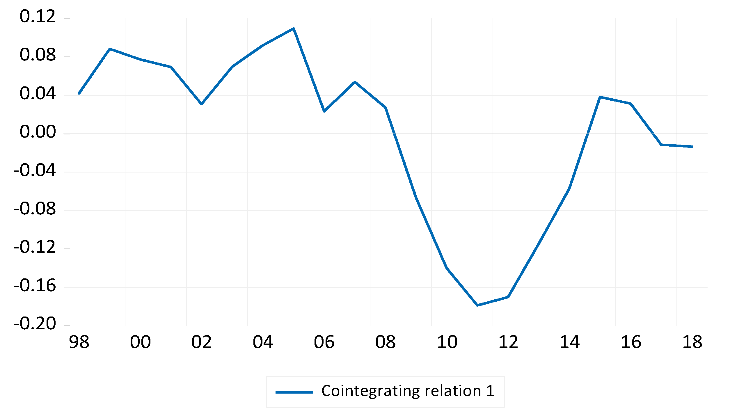
The cointegrating equation presented above is visualized in the graph illustrated in next figure (Figure 2).

It is obvious that the evolution of the cointegrating relation oscillates in positive rates, while in 2009 a decreasing trend is evident, with the lowest value to be recorded for the year 2012. An increasing trend is illustrated after the year 2012, while a positive value of GDP, and thus economic growth, is recorded after the year 2015 with stabilization to follow after the year 2017. The cointegrating equation describes only the evolution of the long-term relationship in a multivariate framework.

The estimation of the Vector Error Correction Model is the econometric tool to describe the short-term dynamics of the methodology, while the results are provided in

Table 5. VECM Estimation results.

Dependent Variables:	D(LG1)	D(LEDU)	D(LDEF)
Independent Variables:
ECT	−0.652832	1.195113	6.244302
	[4.41944]	[2.33917]	[5.36954]
D(LG1(-1))	−0.596407
	[−2.90143]
D(LG1(-2))	−0.776878
	[−4.17149]
D(LEDU(-1))	0.187016
	[2.90040]
D(LEDU(-2))	−0.117060
	[−2.43813]
D(LDEF(-1))	0.139360	0.305032	1.075223
	[3.73082]	[2.36100]	[3.65637]
D(LDEF(-2))	0.073347
	[2.62153]
D(HEAL(-2))	−1.97 × 10−5
	[−3.26219]
C			−0.058172
			[−2.12478]
D_2009	−0.047991
	[−2.96158]
Rsquared	0.901498	0.831227	0.881474
Adj. R-squared	0.766058	0.599165	0.718501

Source: Own Study.

.

Furthermore, and according to the results presented in Table 5, the coefficient of the error correction term is significant for 5% significance level for all the variables employed, with exception that of the government expenses in education. The non-significant variables are not included in the estimated model. In addition, regarding the short-term dynamics, the first lag of expenditures in education and health seems to affect the national income in a positive way; this is not the case for the second lag, for which the relationship estimated is negative. As far as the case for which the sectoral expenses are dependent variables, no statistically significant impact on their formation of national income is validated. Thus, the Keynesian approach is also validated in the short run.

Regarding the residuals of the VECM as presented in

Table 6. Residual Statistics.

	Stat Value	Prob
BG test	15.55281	0.4846
BGP test	105.56	0.66
Probs from chi-square with 16 df.

Source: Own Study.

, we can argue that the residuals of the model do not suffer neither from heteroskedasticity nor from autocorrelation. Furthermore, the fact that the cointegrating equation is significant only in the first equation implies that the value of government expenses for education and health are not affected by the other variables.

A test employed to detect multicollinearity for the Vector Error Correction Model is the Vector Inflation Factors statistics, the results of which are provided in

Table 7. VIF Results.

	Coefficient	VIF Centered
LEDU	0.016733	5.138065
LHealth	0.018526	8.431003
Ldef	0.009458	4.959912

Source: Own Study.

.

Based on the aforementioned results, given that the value of VIF is less than ten for all the variables, no serious problem of multicollinearity is detected that could affect the reliability of the VECM estimation results.

Another step in our analysis that provides interesting results is the pairwise Granger causality test. The particular test is vital in order to determine the validity of the Wagner law or Keynesian approach in the economy under review in a bi-variate framework. The test results are provided

Table 8. Granger Pairwise causality test.

Null Hypothesis:	Obs	F-Statistic	Prob.
LEDU does not Granger Cause LGDP	22	0.30169	0.7434
LGDP does not Granger Cause LEDU		6.45964 ***	0.0082
LHEAL does not Granger Cause LGDP	22	0.03	0.9971
LGDP does not Granger Cause LHEAL		18.6 ***	5 × 10−5
LDEF does not Granger Cause LGDP	22	0.0	0.9419
LGDP does not Granger Cause LDEF		6.3 ***	0.0089
LHEAL does not Granger Cause LEDU	22	5.14453 **	0.0179
LEDU does not Granger Cause LHEAL		0.03040	0.9701
LDEF does not Granger Cause LEDU	22	4.61623 **	0.0250
LEDU does not Granger Cause LDEF		0.14854	0.8631
LDEF does not Granger Cause LHEAL	22	1.28055	0.3034
LHEAL does not Granger Cause LDEF		1.23224	0.3164

Source: Own study. **, *** rejection of null hypothesis for 5 and 1% level of significance.

.

Given that the pairwise causality tests may be employed only on stationary data, the particular tests involve the first differences of the variables studied. The results are provided in Table 8.

The causality based on our findings is directed from GDP to government expenses (health, defense, and education), validating the Wagner Law. These results are not in line to the results based on Johansen cointegration tests in the long and short term.

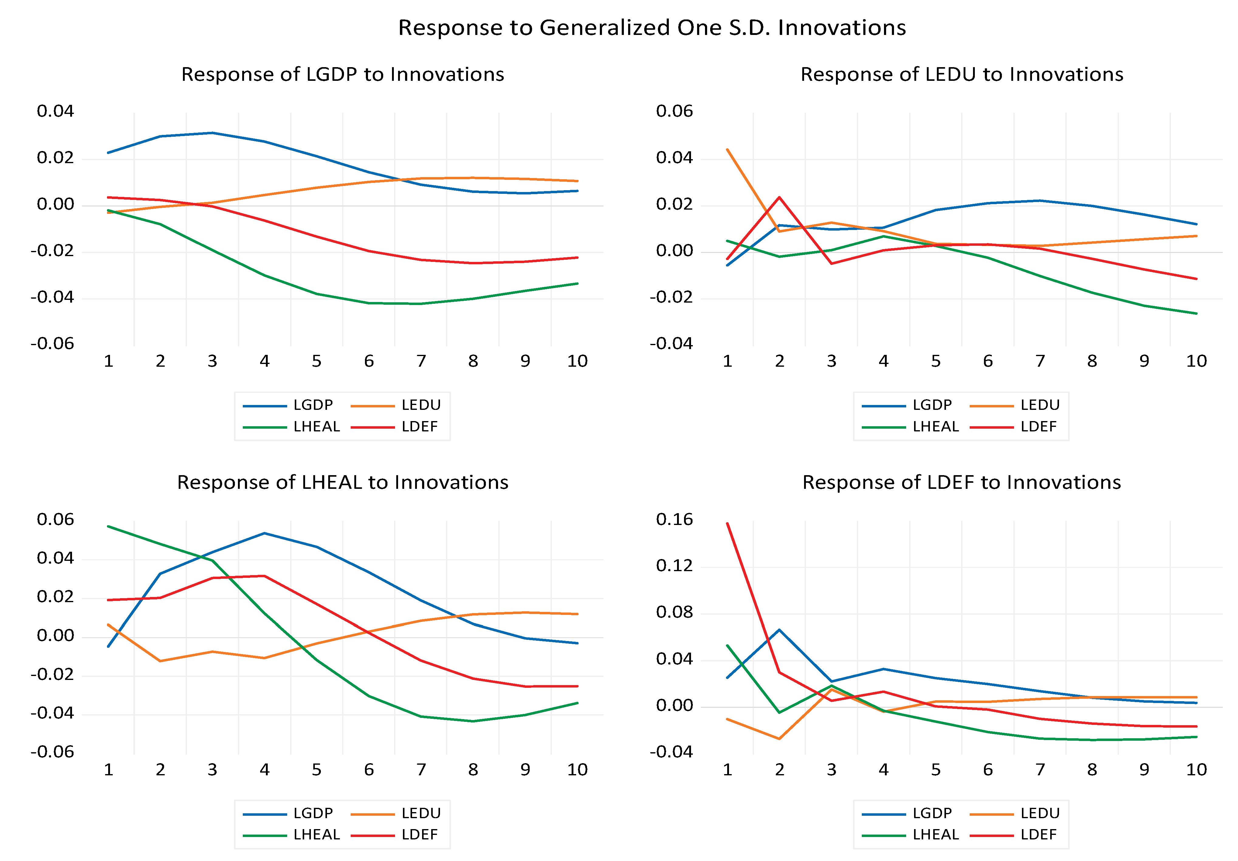
The next step in our analysis involved the impulse response analysis for the variables employed in our model. As mentioned above, this analysis is an important step in order to describe the evolution of a model’s variables in reaction to a shock in one or more variables. Implicitly, this feature allows us to trace the transmission of a single shock within an otherwise noisy system of equations, and thus makes them very useful tools in the assessment of economic policies.

According to the graph provided in Figure 3, for every standard deviation innovation, an initial increase in the GDP is evident that almost disappears after 10 periods. For all the other variables, a similar pattern is confirmed, with an exception for the expenses for defense, which is more inelastic in GDP changes.

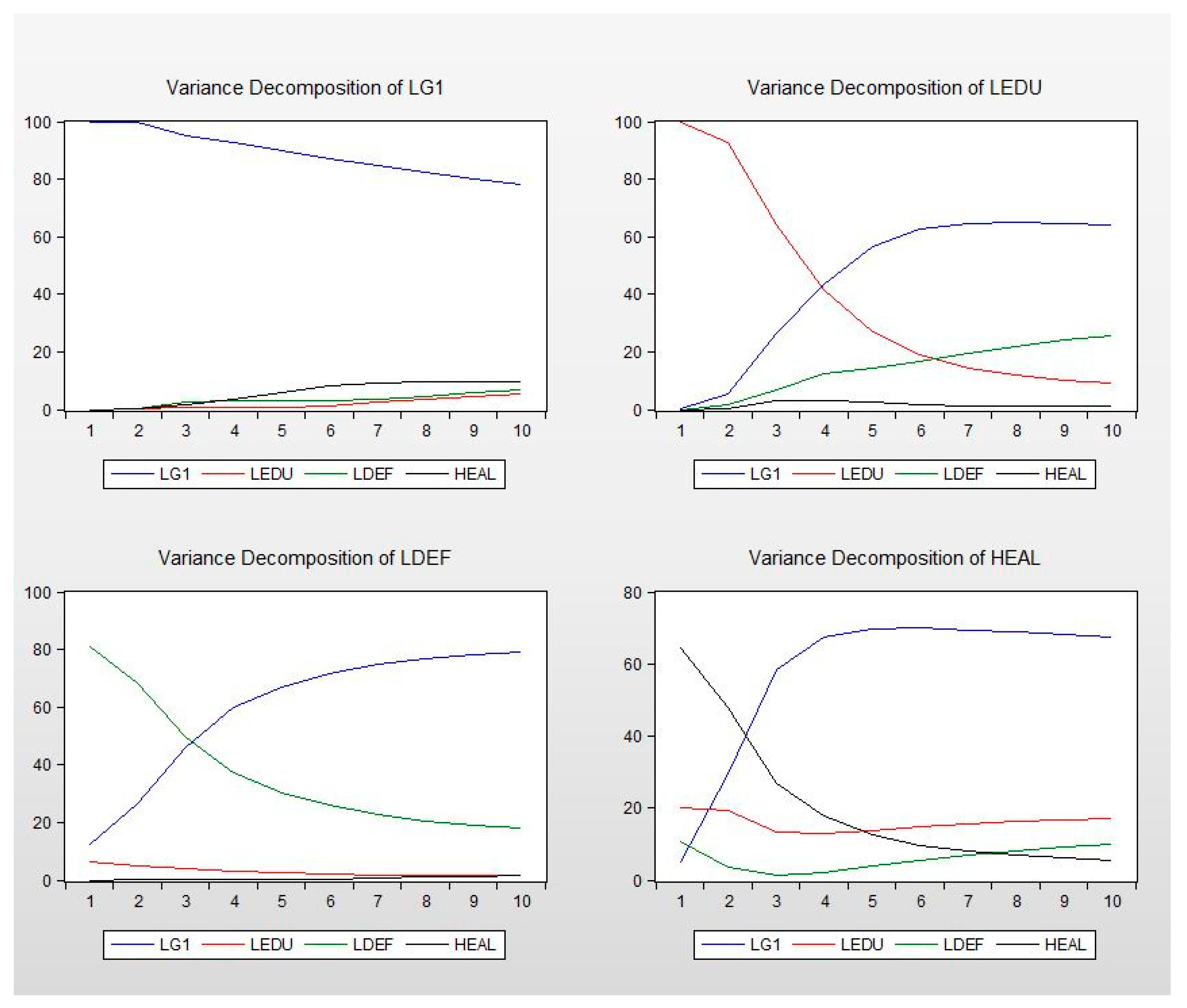
The variance decomposition results are illustrated in Figure 4. The variance decomposition is a necessary procedure in order to determine the proportion of variation of the dependent variable being attributed to each one of the independent variables individually. To be more specific, the first part of the figure involves the variance interpretation of GDP with limited interpretation ability for the following periods, while the education variance is adequately interpreted by variances in the other variables in the following periods in an increasing way. The variance in the case of defense is mainly interpreted by variance in GDP and slightly by the other two variables. The government spending in half variance is interpreted mainly by GDP and much less by education, while government spending for defense is limited.

5. Discussion and Conclusions

The present work examined the sectoral public expenditure–national income relationship in a multivariate framework for a period within which the economy is going through a severe economic crisis, coupled with the economic conditions imposed by the Memorandum since the year 2009. The public expenditures studied involve education, health, and defense. The first two sectoral expenses are considered productive, the expansion of which in the long term entails economic growth, while the defense expenditures may affect economic growth via different routes. More specifically, we examined, with the assistance of the Johansen cointegration, the long-run relationship among the variables under review, while we estimated the Vector Error Correction Model to examine the short-run dynamics of the relationship studied. In addition, with the econometric tool of the Granger pairwise test, we examined causality among the time series employed in a two-variate framework without taking into consideration the interactions of the variables studied. The major objective of the present study was to examine whether under these severe economic conditions the Keynesian approach or Wagner’s law is the appropriate framework to adequately interpret the effectiveness of the economic policy adopted. The Johansen cointegration technique has validated the existence of a sole relationship among the variables employed that we estimated, and in which the national income is the result of interactions among the sectoral public expenses employed in the present model. Thus, the multivariate framework validated the Keynesian approach, a result that is in line with the existing literature as described in Dudzevičiūtė et al. [38], where the public expenses affect national income and economic growth in sequence [38,50,51]. In the case of the EU, the Keynesian approach was validated for the cases of Sweden and Slovakia. In addition, the Vector Error correction model was estimated to capture the short-term dynamics. The expenses for education and public defense do not have a positive impact on the economic growth in the short term. This result implies that education is not a source of economic growth in the short term, and therefore one should seek a potential interpretation for this result. This achievement may well provide policy makers with the ability to enact education as an effective source of economic growth. Regarding the expenses in defense, impacts of conflict on economic growth are possible. Explicitly, economic growth may be limited, given that the particular expense is unproductive public expenditure or limiting the efficiency of the other expenses. On the contrary, military spending could promote economic growth with the tool of ‘military Keynesianism’, or ‘through ‘spillover effects’ from military research and development (R&D) of technologically advanced products to civilian spin-off products’ [10]. As for the expenses for public health, there seems to be a positive impact on economic growth in the short term.

Our findings concerning the multivariate framework in the long and the short term are in line with those of Gisore [40] that confirmed the Keynesian approach for East African countries and found no significant impact for the public expenses of education on national income. In addition, in the case of Spain [52], the law of Wagner is validated for health, education, and defense, while the reversed direction of causality is confirmed for the public expenses on health. Concerning previous works that examined the validity of Wagner Law in the case of Greece, the results obtained by Antoniou et al. [11] for long data over a century are not in line with the findings of the present study since they confirmed the Wagner Law in the long term, with a few exceptions for certain periods. The Wagner Law has also been confirmed for data extending for the ninetieth century by Sideris [44] that did use disaggregated data for public expenses. Therefore, the present work differs from the theoretic framework according to which the effect of ‘productive public expenditures’, namely education and health, should be positive for growth and poverty reduction [51,52,53].

On the other hand, concerning the results of the Granger causality pairwise tests being performed, it becomes evident that the national income is the variable that determines both productive sectoral public expenditures, namely health and education, a result that validates the Wagner Law in a two-variate framework. The particular results are in line with all the studies for Greece on the validity of Wagner Law [11,44].

The aforementioned analysis and the comparison of the two-variate and multivariate framework implies that the proper allocation of the sectoral public expenses by the government may well promote economic growth, while the different results derived for the two-variate framework may be attributed to a lack of information on the interactions concerning the total economy, especially the productive public expenses.

Another issue that should be stressed and may interpret our findings is related to the fact that, the economic crisis within the European Union has led the governments in the name of the Stability and Growth Pact to implement strict fiscal rules, limiting in sequence the government’s ability to exercise public management [54,55,56,57,58,59,60,61]. Furthermore, in our study concerning Greece an economy with a number of particularities such as bureaucracy, huge public debt, and the Memorandum in valid formulate an economic environment vulnerable to economic shocks either related to the pandemic or to other sources [1]. All these results should be further analyzed in order for policy makers to become able to seek routes and tools to enhance economic growth via the appropriate public expenditures allocation securing profitable investments, in different sectors of the economy.

A limitation of the present manuscript involves lack of confidence interval estimation in the process of impulse response analysis due to the software applied though this not restraining the valuable findings of the present work for policy makers.