Boosting Arithmetic Optimization Algorithm with Genetic Algorithm Operators for Feature Selection: Case Study on Cox Proportional Hazards Model

Abstract

Feature selection is a well-known prepossessing procedure, and it is considered a challenging problem in many domains, such as data mining, text mining, medicine, biology, public health, image processing, data clustering, and others. This paper proposes a novel feature selection method, called AOAGA, using an improved metaheuristic optimization method that combines the conventional Arithmetic Optimization Algorithm (AOA) with the Genetic Algorithm (GA) operators. The AOA is a recently proposed optimizer; it has been employed to solve several benchmark and engineering problems and has shown a promising performance. The main aim behind the modification of the AOA is to enhance its search strategies. The conventional version suffers from weaknesses, the local search strategy, and the trade-off between the search strategies. Therefore, the operators of the GA can overcome the shortcomings of the conventional AOA. The proposed AOAGA was evaluated with several well-known benchmark datasets, using several standard evaluation criteria, namely accuracy, number of selected features, and fitness function. Finally, the results were compared with the state-of-the-art techniques to prove the performance of the proposed AOAGA method. Moreover, to further assess the performance of the proposed AOAGA method, two real-world problems containing gene datasets were used. The findings of this paper illustrated that the proposed AOAGA method finds new best solutions for several test cases, and it got promising results compared to other comparative methods published in the literature.

1. Introduction

Datasets of broad sizes exist in several real data applications such as pattern recognition, data mining, signal processing, machine learning, text processing, image processing, and web content classification [1,2,3]. These datasets typically contain a significant range of hard-to-cope features. As a result, the quality of these applications’ performance is often decreased by redundant, noisy, and meaningless data [4,5,6].

Researchers used dimensional reduction to eliminate the unimportant and redundant data, which maps the original high-dimensional space data into new lower-dimensional space data [7,8]. Reducing dimensional also allows to imagine and reflect the data and can increase the application’s output [9]. Feature selection is one of the most common strategies used in the dimensional reduction domain to solve the dimensional problem. The goal of handling features is to represent, with high precision, the original features in a specific problem domain by an optimal subset of new selected features [10]. It is possible to execute the feature selection process in the backward or forward direction. The backward selection strategy collects all characteristics; it then eliminates one attribute at each step (whose removal reduces the error the most). This method is replicated until some further elimination increases the fault [11,12]. The forward selection strategy starts with a blank set; it adds one element at each stage that reduces the error the most before another addition does not mainly reduce it [13,14].

There are two types of feature selections, filter and wrapper methods in general; the critical distinction between them is in the technique of choosing the subset of new features [15]. To test the feature subset, the wrapper approaches used the learning methodology. However, it is not feasible to use the wrapper to work with a high-dimensional dataset. This is because the related features require significant time to be decided. However, unlike wrapper approaches, the filter strategy does not use learning techniques to select the features. For these purposes, the wrapper is costly for computing, so it can not be extended to large-size files. In comparison, filter algorithms are also less expensive in terms of computing [16,17].

The feature cost, which means the cost of obtaining a feature attribute, is a particular case in machine learning and data mining with different cost types. It can be portrayed in different ways, such as income, time, pain, and measurement cost, to say a few [18,19,20]. In medical diagnosis, it is usually inexpensive and painless to obtain the values of symptom characteristics detected through the eyes or even cost less. However, getting the importance of other diagnostic characteristics often poses varying costs and risks due to the need to perform several clinical examinations. These expenses are either resources or time for test results or the patient’s medical and psychological pressures. Improving the diagnostic effect by choosing many critical characteristics is essential for this problem. However, it is also necessary to increase the comfort level by choosing cost-less features or saving money. In this case, before settling on the selected diagnostic features, a doctor needs to estimate the trade-off between the diagnostic impact and the cost. In real-world implementations, there are several related examples. However, most of the conventional feature selection approaches neglect the question of the expense of the function [21,22].

When all possible subsets of the dataset are removed during the generation process, there is very high complexity and a high processing time of $x^2$, where x is the number of characteristics in the dataset [23]. Therefore, physicists have sought to formulate approaches to solve the feature selection (FS) problem and provide solutions more efficiently than conventional techniques. This problem is considered one of the most recent problems faced by the new technology due to the size of the available information and data [24,25,26]. The use of metaheuristic algorithms is one such approach. On many topics in artificial intelligence, metaheuristic algorithms have been applied and have led to many solutions [27,28,29]. To solve feature selection problems, metaheuristic algorithms are now widely used [30]. According to parameters governed by the way these algorithms operate, they generate subsets randomly. It has been shown that they can help minimize execution time and produce specific outcomes. Grey Wolf Optimizer (GWO) [31], Whale Optimization Algorithm [32], Monarch Butterfly Algorithm [23] Coyote Optimization Algorithm [33], Genetic Algorithm [34], Krill Herd Algorithm [35] Harmony Search [36], Aquila Optimizer [37], Particle Swarm Algorithm [38], and Parallel Membrane-inspired Framework [39] are examples of the metaheuristics that have been used to address feature selection problems.

In the literature, several techniques have been published [40,41,42,43,44], such as, in this paper, the enhancement is carried out by integrating the opposition-based learning methodology, and differential evolution with the Moth-flame Optimization (MFO) [15]. To maximize the integration of the MFO, opposition-based learning is used to produce an optimum initial population; meanwhile, the differential evolution is applied to boost the MFO’s ability to manipulate. Therefore, unlike the conventional MFO algorithm, the suggested approach noted as OMFODE avoided getting trapped in an optimal local value and increase the rapid convergence. This paper proposes a hybrid solution that incorporates two search methods: GWO and Particle Swarm Optimization (PSO) [45]. The GWO is stimulated by the leadership hierarchy and the gray wolves’ hunting actions in nature, with gray wolves choosing to live in a pack. The goal of this hybridization is to combine exploitation and exploration in a balanced manner.

In the paper [23], the novel monarch butterfly optimization (MBO) algorithm is implemented with a wrapper feature selection approach that uses the classifier k-nearest neighbor (KNN). On eighteen benchmark datasets, tests are introduced. The results showed that MBO was superior to four optimization algorithms, providing a high accuracy rate in classification. For feature selection challenges of medical diagnosis and other problems in this paper, a hybrid crow search algorithm is developed and integrated with chaos theory and fuzzy c-means technique designated as CFCSA [46]. The crow search algorithm adopts the global optimization methodology in the recommended CFCSA context to prevent local optimization’s sensitivity. As a cost attribute for the messy crow search algorithm, the fuzzy c-means (FCM) target function is used. Like other optimization algorithms, the Salp Swarm Algorithm (SSA) suffers from population diversity and crashes into the local optimum. This research provides an improved SSA variant known as the Dynamic Salp swarm algorithm to solve these problems (DSSA) [47]. To fix its challenges, two significant changes were included in the SSA. The first upgrade entails creating a new equation for updating the location of salps. By using Singer’s chaotic map, the use of this new equation is regulated. The first change aims to increase the diversity of SSA solutions. The second enhancement entails creating a new local search algorithm (LSA) to increase the exploitation of SSA.

As discussed beforehand, optimization algorithms have shown promising effects when used to address the feature selection problems in recent decades. However, considering increasing research in this direction, whether we need further optimization approaches to find more enhanced outcomes, a fundamental question still emerges. In this regard, these newly introduced metaheuristic algorithms, derived from arithmetic operators, biological evolution, swarm behavior, physical concepts, and mathematical laws, have been increasingly investigated. However, researchers claim that these approaches frequently work ineffectively when there is a substantial increase in complexity and problem dimensionality. This research has two primary motivations: (A) No-Free-Lunch (NFL), which states that there is no optimization technique to solve all optimization problems, so the optimizer’s outstanding success on a specific group of problems does not guarantee another group of problems perform equally effectively. This has inspired many scientists in this area to apply the current approaches to new problem groups. The same is the basis and inspiration for this research. We suggest a novel optimization method by integrating the Arithmetic Optimization Algorithm (AOA) and the operators (Crossover and Mutation) of the Genetic Algorithm to solve the feature selection problem with higher dimensionality. This problem can be categorized as hard, and it can not be solved easily by a traditional technique. So, it needs an advanced and improved method to find the optimal solution for the used cases in this paper. (B) To the best of the developers’ understanding, the proposed method is used for the first time to solve the feature selection problems. The proposed method tackled the conventional AOA’s main weaknesses by avoiding the search strategies’ local search problem and search balancing. As the optimization methods are the best choice to deal with such a complicated problem, we use the proposed method according to its previous performance with some improvements to efficiently tackle the feature selection problem and find a new best solution. Twenty feature selection datasets are used to prove the proposed method’s performance, and the results are compared with other state-of-the-art methods using the standard evaluation criteria. The results showed that the proposed method’s ability is promising in solving the high-dimensional feature selection problems compared to other well-known methods.

The main contributions invented in this paper are given as follows.

• A modified approach of the classical AOA and GA is proposed that further enhances the exploration and convergence characteristics of this evolutionary-based wrapper feature selection method through the diverse population design.
• Boosted mutation and crossover operators are introduced for search-based exploration and exploitation of the search.
• The GA operator’s inclusion promotes the convergence rate to balance the exploration and exploitation characteristic of the proposed approach.
• Decrease of the feature input set using the proposed search method for high dimensional problems is conducive to develop a high-performing decision method.
• Comparing the proposed method with several state-of-the-art methods on twenty datasets is conducted.

The design of the rest of this paper is as follows. Section 2 shows the general methods and the proposed improved algorithm. Then, Section 3 presents the experiments and the discussion of the results. Finally, Section 4 gives a conclusion of this paper and potential future directions works.

2. Methods

2.1. Problem Formulation of FS

In this section, the mathematical formulation of FS is introduced. In general, the classification (i.e., supervised learning) of any datasets which has size $N_S\times N_F$ where $N_S$ is the number of samples and $N_F$ stand for the number of features. The main objective of FS problem is to select a subset of features S from total number of features ($N_F$) where the size of S is less than $N_F$. This can be achieved by minimizing the following objective function:

$$Fit=\lambda \times {\gamma }_S+(1-\lambda )\times \left(\frac{\left|S\right|}{N_F}\right)$$

(1)

where ${\gamma }_S$ refers to the classification error using S and $\left|S\right|$ are the number of selected features. $\lambda$ is used to balance between $\left(\frac{\left|S\right|}{N_F}\right)$ and ${\gamma }_S$.

2.2. Arithmetic Optimization Algorithm (AOA)

The preliminaries of the AOA [48] are described in this section. Generally, like other MH algorithms, the AOA has two search phases, exploration, and exploitation, inspired by mathematics operations, such as $-,+,\ast$, and /. First, the AOA generates a set of N solutions (agents). Each one represents a solution for a tested problem. Thus, solutions or agents represent X population, as:

$$X=\left[\begin{array}{ccccc}{x}_{1,1}& \cdots & x_{1,j}& x_{1,n-1}& x_{1,n}\\ x_{2,1}& \cdots & x_{2,j}& \cdots & x_{2,n}\\ \cdots & \cdots & \cdots & \cdots & \cdots \\ ⋮& ⋮& ⋮& ⋮& ⋮\\ x_{N-1,1}& \cdots & x_{N-1,j}& \cdots & x_{N-1,n}\\ x_{N,1}& \cdots & x_{N,j}& x_{N,n-1}& x_{N,n}\end{array}\right]$$

(2)

Next, the fitness function of each solution is computed to detect the best one $X_b$. Then, depending on the Math Optimizer Accelerated ($MOA$) value, AOA performs exploration or exploitation processes. Then, $MOA$ is updated as the following equation:

$$MOA\left(t\right)=Min+t\times \left(\frac{Ma{x}_{MOA}-Mi{n}_{MOA}}{M_t}\right)$$

(3)

in which $M_t$ represents the total number of iterations. $Mi{n}_{MOA}$ and $Ma{x}_{MOA}$ represent the minimum and maximum values of the accelerated function, respectively. More so, the multiplication (M) and division (D) are employed in the exploration phase of the AOA, as presented in the following equation:

$$X_{i,j}(t+1)=\left\{\begin{array}{cc}{X}_{bj}÷(M_{OP}+ϵ)\times ((U{B}_j-L{B}_j)\times \mu +L{B}_j),& r_2<0.5\\ X_{bj}\times M_{OP}\times ((U{B}_j-L{B}_j)\times \mu +L{B}_j),& otherwise\end{array}\right.$$

(4)

in which $ϵ$ represents a small integer value, $U{B}_j$ and $L{B}_j$ are the lower and upper boundaries of the search domain at jth dimension. $\mu =0.5$ represents the control function. Moreover, Math Optimizer ($M_{OP}$) can be described as:

$$M_{OP}\left(t\right)=1-\frac{t^{1/\alpha }}{M_t^{1/\alpha }}$$

(5)

$\alpha =5$ represents the dynamic parameter that determines the precision of the exploitation phase throughout iterations.

Furthermore, addition operators (A) and subtracting (D) operators are used to implement the AOA exploitation phase, using the following equation.

$$x_{i,j}(t+1)=\left\{\begin{array}{cc}{X}_{bj}-M_{OP}\times ((U{B}_j-L{B}_j)\times \mu +L{B}_j),& r_3<0.5\\ X_{bj}+M_{OP}\times ((U{B}_j-L{B}_j)\times \mu +L{B}_j),& otherwise\end{array}\right.$$

(6)

In which $r_3$ represents a random number generated in [0,1]. After that, the agents’ updating process is implemented using the AOA operators. To sum up, Algorithm 1 illustrates the main steps of the AOA.

Algorithm 1 Steps of AOA

1: Input: The parameters of AOA such as dynamic exploitation parameter ($\alpha$), control function ($\mu$), number of agents (N) and total number of iterations $M_t$.  2: Construct the initial value for the agents $X_i$ $i=1,...,N$.  3: while ($t<M_t$) do  4:  Compute the fitness function for each agent.  5:  Determine the best agent $X_b$.  6:  Update the $MOA$ and $M_{OP}$ using Equation (3) and Equation (5), respectively.  7:  for $i=1$ to N do  8:   for $j=1$ to $Dim$ do  9:    Update the value of $r_1$, $r_2$, and $r_3$. 10:    if $r_1>MOA$ then 11:     Exploration phase 12:     Use Equation (4) to update the $X_i$. 13:    else 14:     Exploitation phase 15:     Use Equation (6) to update the $X_i$. 16:    end if 17:   end for 18:  end for 19:  t = t + 1 20: end while 21: Output the best agent (feature subset) ($X_b$).

2.3. Genetic Algorithm

In this section, the basic information of Genetic algorithms (GA) is introduced [49]. In general, GA is a population-based meta-heuristic technique, and each individual inside the population represents a feasible solution. There are three stages in GA used to update the individuals, namely Selection, Crossover, and Mutation process. In the Selection process, two individuals are selected randomly, which leads to enhancing the population’s diversity. Then the crossover process generates new individuals from the selected individuals (parents) by exchanging their values. After that, the mutation is applied to replace a randomly selected individual with a random value belonging to the search space. Finally, according to the fitness value of newly generated individuals and their parents, the current population is updated by selected the best individuals to form the new population. Then, updating the population using the three processes of GA (i.e., selection, crossover, and mutation) is repeated until reached the stop conditions.

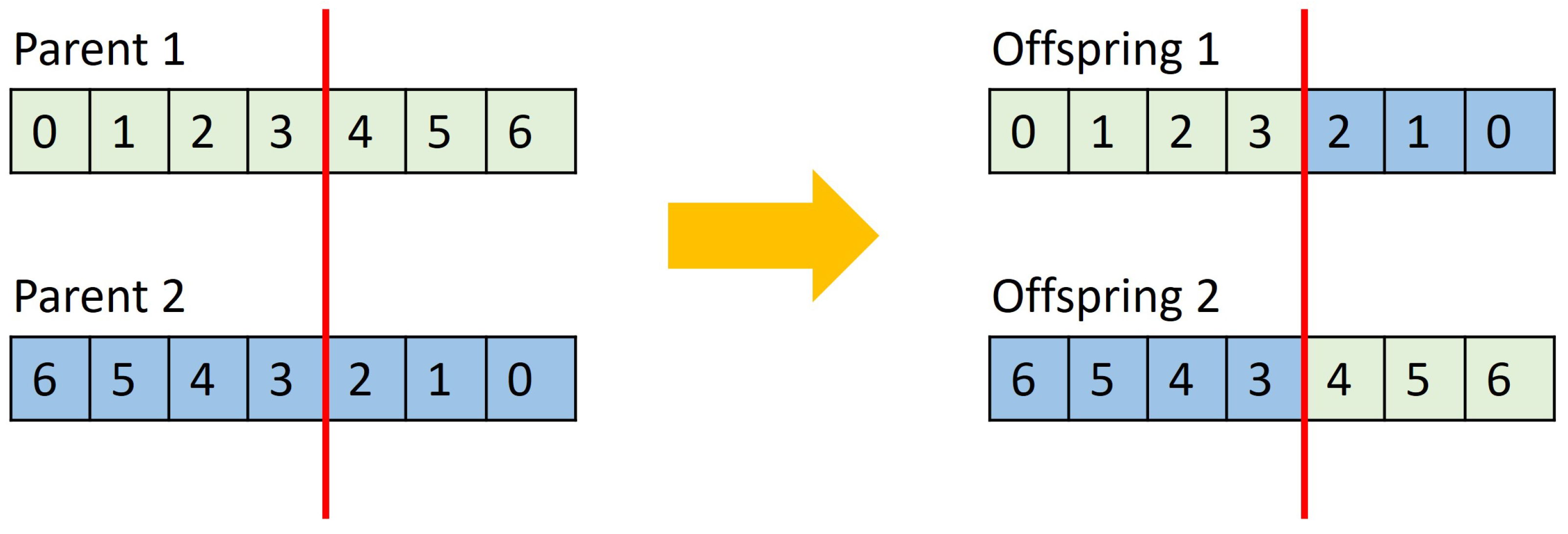
2.3.1. Crossover

One of basic operators in GA is the crossover, in the related literature they are different modification of it. The most simple crossover is the single point method. Here are necessary two parents that are randomly selected from the population. The parents are used to generate an offspring by sing a single point that divides the information contained in them. By using a single points the values after it are interchanged between the two parents and new solutions are created. The Figure 1 graphically shows how the single point crossover works.

The single point crossover is a good alternative, but for real code purposes it is better to employ another version. The blend crossover also known as BLX-$\alpha$ is a real coded operator. Similar to the single point, it is necessary to take two parents $x^1$ and $x^2$ from the population. By using the parents it is extracted a portion $x_i^c$ from bot of them. Equation (7) provides a better explanation of BLX-$\alpha$.

$$\begin{array}{c}{X}_i^1=min\left(x_i^1,x_i^2\right)-\alpha d_i\hfill \\ X_i^2=max\left(x_i^1,x_i^2\right)-\alpha d_i,\hfill \\ d_i=\left|x_i^1-x_i^2\right|\hfill \end{array}$$

(7)

where, $x_i^1$ and $x_i^2$ are elements taken from $x^1$ and $x^2$ and $\alpha$ is positive value setting to $0.5$ according to [50].

2.3.2. Mutation

The mutation is an operator that helps to explore around of an specific solution. Similar to the crossover they are several ways to perform the mutation. However, in this article it is considered the Gaussian mutation that was introduced by Higashi and Iba [51]. In this kind of mutation it is necessary to take an element form the population and it is modified by using a random number created by a Gaussian distribution. The modified solution is a mutated individual and it is computed as follows:

$$mutate\left(x_{id}\right)=x_{id}\times (1+gaussian\left(\sigma \right))$$

(8)

From Equation (8) $x_{id}$ is the selected individual from the population, Gaussian ($\sigma$) is a random number generator that uses a Gaussian distribution with a standard deviation of $\sigma =0.1$.

2.3.3. Selection

The selection operator is also important because it helps to extract the elements of the population that will be manipulated by the crossover and mutation. Here is also possible to find different mechanisms but the most common is the roulette wheel [52]. This method is based on the fitness and it works by assigning a probability $ps$ to a each member of the population. The population then is segmented into different regions represented by the individuals. In a population of n candidate solutions defined as $P=\left\{a_1,a_2,\dots ,a_n\right\}$ the element $a_i$ possesses a fitness value $f\left(a_i\right)$, then the probability of $a_i$ to be selected is computed as:

$$ps\left(a_i\right)=\frac{f\left(a_i\right)}{{\sum }_{i=0}^{n}f\left(a_j\right)},j=1,2,...,n$$

(9)

3. Proposed AOAGA Feature Selection

Optimization techniques, as mentioned above, have been successfully used in many research fields to solve various complicated problems. In this section, the proposed optimization method is presented to solve the feature selection problems. This problem is a widespread complex issue that has appeared in many knowledge-based approaches, and it needs an efficient method to solve. It is typically based on selecting the optimized features from a massive amount of features to reduce the computational time and increase the performance of the underlying system analysis.

Figure 2 depicts the structure of the developed feature selection method. This method depends on enhancing the performance of AOA to find the optimal subset of relevant features using the operators of the genetic algorithm (GA).

The developed FS method is called AOAGA. The main difference between AOAGA and the original AOA is that the exploration phase of the proposed AOAGA is improved and can explore more regions in the search domain than the original version of the AOA, and it also can escape from getting stuck in local optima due to operators of the GA.

The AOAGA starts by setting the initial population U, which has N number of agents; this formulated using the following:

$$U_i=L{B}_i+{\alpha }_i\times (U{B}_i-L{B}_i).$$

(10)

In Equation (10), ${\alpha }_i\in [0,1]$ is a random value. The $U{B}_i=1$ and $L{B}_i=0$ are limits the search domain. The next step in the developed AOAGA is to assess the quality of the selected feature. This is achieved by converting each agent into the binary form using the following equation.

$$B{U}_{ij}=\left\{\begin{array}{cc}1& if{U}_{ij}>0.5\\ 0& otherwise\end{array}\right.$$

(11)

Thereafter, computing the classification error after removing the irrelevant features that corresponding to zeros in $BU$. This is performed by using Equation (12).

$$Fi{t}_i=\lambda \times {\gamma }_i+(1-\lambda )\times \left(\frac{|B{U}_i|}{N_F}\right)$$

(12)

In Equation (12), $\lambda \in [0,1]$ refers to the weight applied to balance between the two sides of Equation (12). $N_F$ refers to the number of features, and $|B{U}_i|$ is the number of selected features corresponding to ones inside $U_i$. ${\gamma }_i$ is the classification error using the features in $U_i$ and is computed based on the KNN classifier. In this study, KNN is learned using a training set representing 80% while the rest dataset is used as a testing set (20%) to evaluate the learned KNN.

Thereafter, the best agent $U_b$ is determined and used to update the other agents with the operators of GA and AOA. This updating process is performed using Equation (13).

$$U_i=\left\{\begin{array}{cc}OperatorsofGA& ift<0.10\times t_{max}\\ OperatorsofAOA& otherwise\end{array}\right.$$

(13)

The next step is to check the stop conditions if they are not met and then repeat the updating process. Otherwise, the best agent is returned and updated the testing set according to it and evaluates the classification’s quality using the updated testing set. The flowchart of the developed AOAGA is given in Figure 2.

The selected primary references in this paper are chosen according to their importance and results in this field. We focused on the most related research in this field to support our research and get significant results and descriptions. However, the main limitations of the proposed method in this paper are selecting real-word feature selection problems for other medical purposes and compared with other advanced methods published in the literature in this domain. This process can further prove the ability of the proposed method to solve various feature selection problems.

The complexity of the developed AOAGA depends on some parameters such as number of agents N, total number of iterations $M_t$, and the dimension of the tested problem n. So, the complexity of AOAGA in terms of Big O can be formulated as:

$$O\left(AOAGA\right)=O(M_{t1}\times N\times N_F)+O\left(M_{t2}(N\times N_F+N\times N_F+N)\right)$$

(14)

Since $M_{t2}=M-M_{t1}$, so we can rewrite Equation (14) as:

$$O\left(AOAGA\right)=O(M_{t1}\times N\times N_F)+O\left((M-M_{t1})(2N\times N_F+N)\right)$$

(15)

$$O\left(AOAGA\right)=O(N\times (M(2N_F+1)-M_{t1}(N_F+1))$$

(16)

where $M_{t1}$ stand for the number of iterations used to update solutions using operators of GA.

4. Experimental Results and Discussion

In this study, the developed AOAGA to improve the performance of classification data is evaluated by removing the irrelevant features. This was achieved using twenty UCI machine learning repository datasets [53] and real-world datasets from [54,55].

The developed AOAGA is compared with ten metaheuristics techniques including Slime mould algorithm (SMA) [56], Harris hawks optimization (HHO) [57], GA [58], Multi-verse optimizer (MVO) [59], SSA [60], MFO, Grasshopper optimization algorithm (GOA) [61], PSO, and GWO [62]. Each algorithm is used with the same parameters used in its original implementation.

These algorithms are run on an 8 GB RAM Intel Core i5 processor using Matlab 2014b. The population is set to 25 whereas, the max number of iterations is 100. Thirteen independent runs are produced for each algorithm.

4.1. Performance Measures

To validate the performance of developed AOAGA, a set of evaluation metrics is used. For example, accuracy, number of selected features, the average and standard deviation of fitness value [63,64,65]. The definition of each measure is given as:

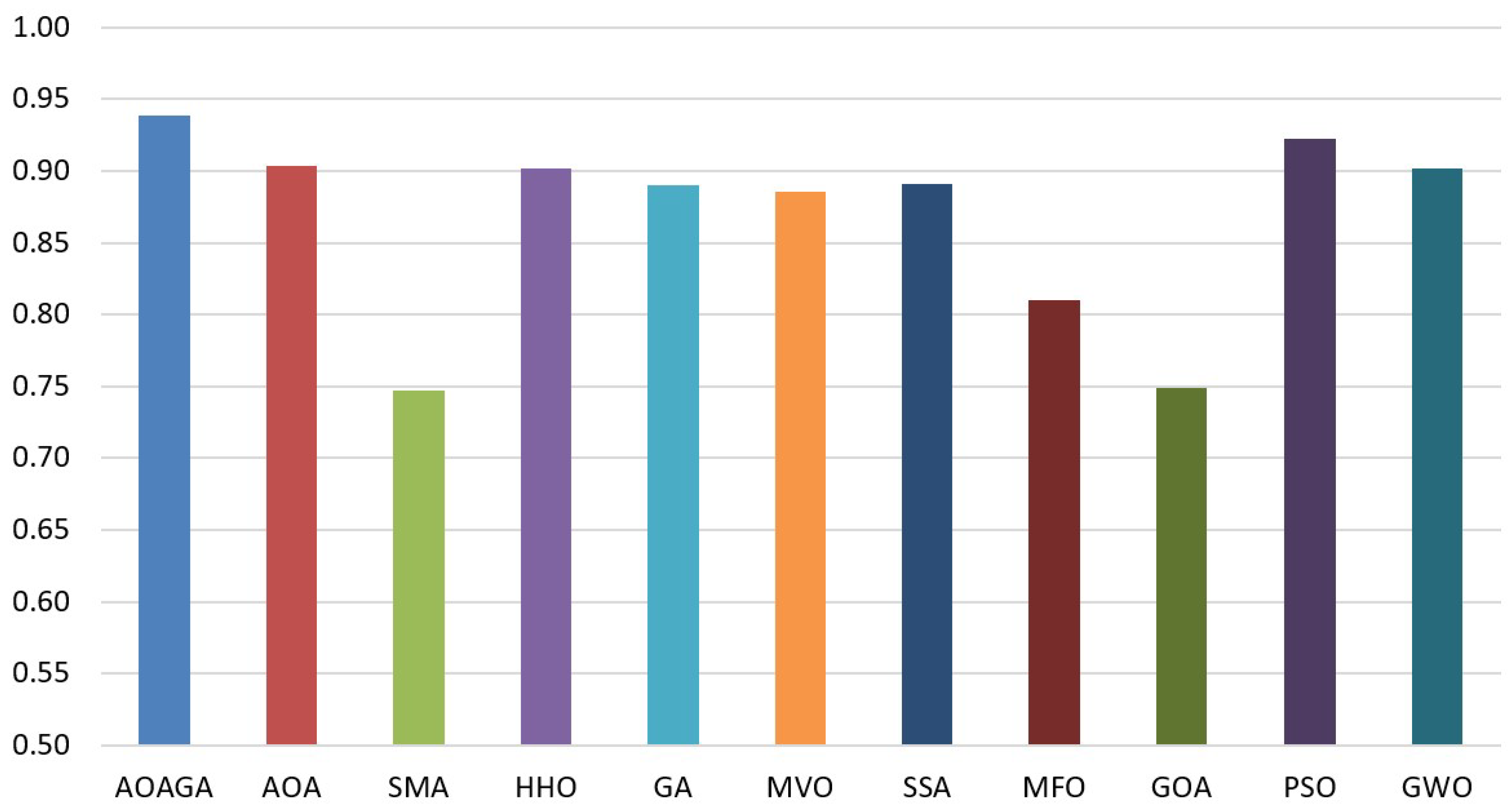
• Average of accuracy $\left(Av{g}_{acc}\right)$ is used to compute the ability of an algorithm to predict the correct label of each class over the runs. Higher value is better [65]. It is defined as:

  $$Av{g}_{acc}=\frac{1}{N_r}\sum _{k=1}^{N_r}Ac{c}_{Best}^k,Ac{c}_{Best}^k=\frac{TP+TN}{TP+FN+FP+TN}$$

  (17)
• Standard deviation (STD) is used to check to what extent an algorithm can obtain the same results over different runs. Smaller value is better [65]. It is formulated as:

  $$ST{D}_Y=\sqrt{\frac{1}{N_r}\sum _{k=1}^{N_r}{\left(Ac{c}_{Best}^k-Av{g}_{acc}\right)}^2}$$

  (18)
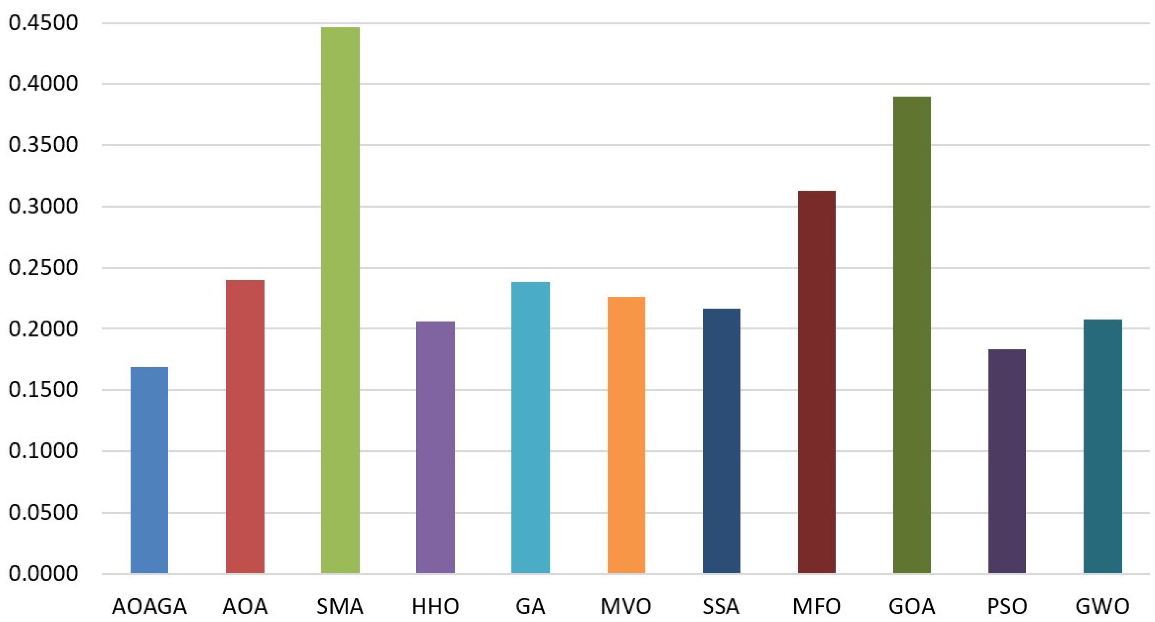
• Average of selected features $\left(AV{G}_{|B{X}_{Best}|}\right)$ is applied to test an algorithm’s ability to choose the smallest subset of relevant features overall runs. Smaller value is better [65]. It is given as:

  $$AV{G}_{\left|B{X}_{Best}\right|}=\frac{1}{N_r}\sum _{k=1}^{N_r}\left|B{X}_{Best}^k\right|$$

  (19)

  where $|.|$ denotes the cardinality of $B{X}_{Best}^k$ at k-th run.
• Average of fitness value $\left(AV{G}_{Fit}\right)$ evaluates the algorithm ability to balance the lower error and ratio of selected features. Smaller value is better [65]. It is formulated as:

  $$AV{G}_{Fit}=\frac{1}{N_r}\sum _{k=1}^{N_r}Fi{t}_{Best}^k$$

  (20)

  where $TP$ and $TN$ refer to the true positive and true negative. Whereas $FN$ and $FP$ are the false positive and false negative, respectively [66].

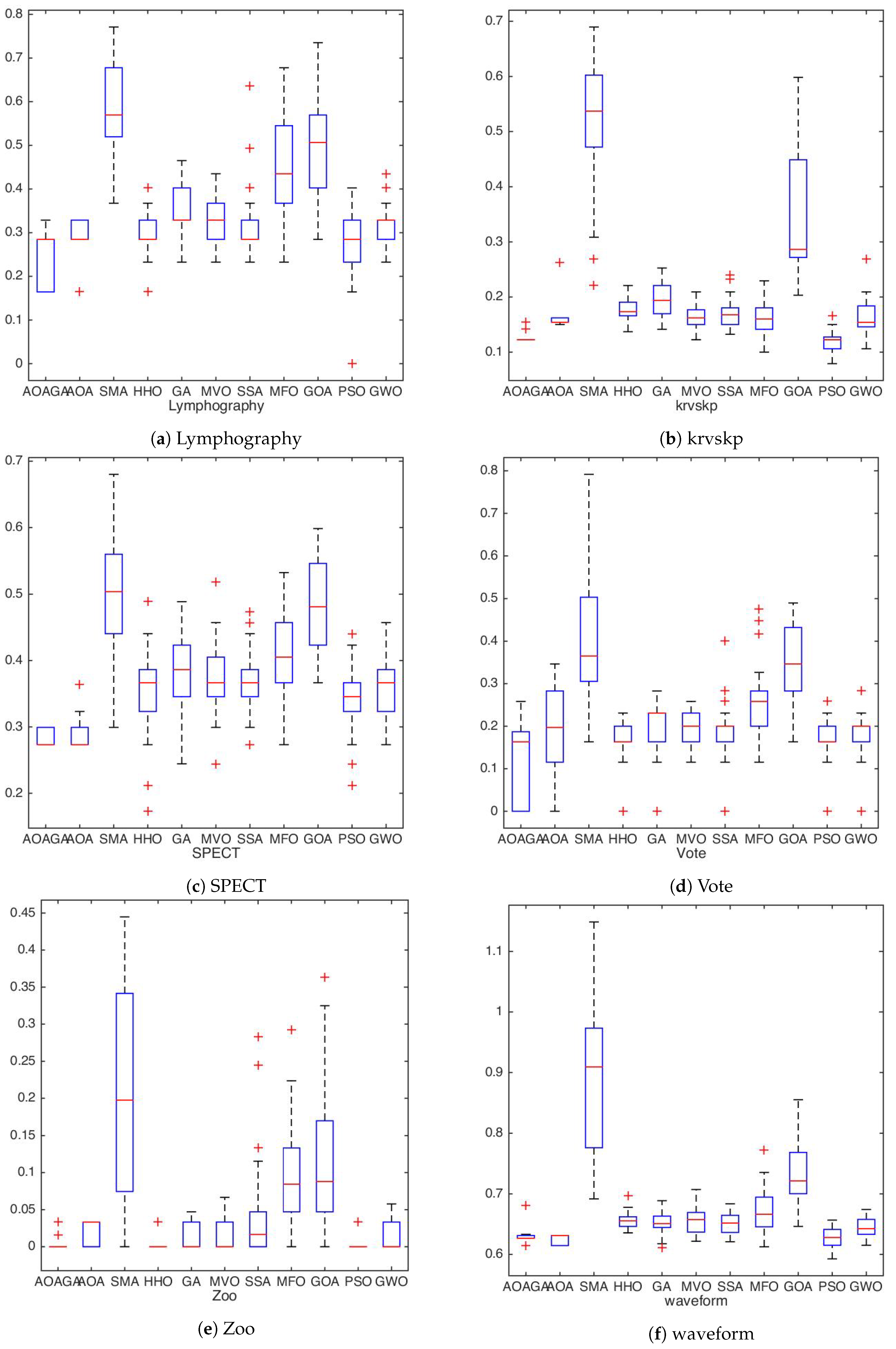
4.2. Experimental Series 1: UCI Datasets Results and Discussion

Within this experiment, a set of UCI datasets are used. These datasets are collected from different fields such as Biology, Game, Electromagnetic, Politics, Physics, and Chemistry. In addition, each of them has a different number of samples, features, and classes. The description of each dataset is given in

Table 1. Description of the benchmark datasets.

Name	Number of Features	Number of Instances	Number of Classes	Data Category
breastWDBC	30	569	2	Biology
ionosphere	34	351	2	Physical
wine	13	178	3	Chemistry
breastcancer	9	699	2	Biology
sonar	60	208	2	Biology
glass	9	214	7	Physics
tic-tac-toe	9	958	2	Game
Lymphography	18	148	2	Biology
waveform	40	5000	3	Physics
clean1data	166	476	2	Artificial
Zoo	16	101	6	Artificial
SPECT	22	267	2	Biology
ecoli	7	336	8	Biology
CongressEW	16	435	2	Politics
M-of-n	13	1000	2	Biology
Exactly	13	1000	2	Biology
Exactly2	13	1000	2	Biology
Vote	16	300	2	Politics
heart	13	270	2	Biology
krvskp	36	3196	2	Game

.

4.2.1. Results and Discussion of UCI Dataset

This subsection presents and discusses the experimental results and comparisons obtained in solving the problem of feature selection. The comparisons used the standard AOA, SMA, HHO, GA, MVO, SSA, MFO, GOA, PSO, and GWO with the metrics described in the previous sections. In

Table 2. Results of the Fitness values for all methods.

Dataset	AOAGA	AOA	SMA	HHO	GA	MVO	SSA	MFO	GOA	PSO	GWO
breastWDBC	0.0968	0.1107	0.3503	0.1207	0.1261	0.1329	0.1122	0.1754	0.2134	0.1058	0.1080
ionosphere	0.1567	0.2086	0.3920	0.2049	0.2262	0.2167	0.2213	0.2704	0.3201	0.1828	0.1803
wine	0.0000	0.0480	0.1858	0.0067	0.0151	0.0194	0.0610	0.1252	0.1578	0.0043	0.0117
breastcancer	0.1620	0.2216	0.3947	0.1898	0.2159	0.2140	0.2082	0.2580	0.3293	0.1682	0.1640
glass	0.1406	0.1452	0.2183	0.1434	0.1520	0.1492	0.1499	0.1879	0.2203	0.1419	0.1451
sonar	0.1387	0.2232	0.4116	0.2065	0.2083	0.1769	0.1885	0.2703	0.3332	0.1204	0.1423
Lymphography	0.2547	0.3261	0.5342	0.3054	0.3561	0.3245	0.3188	0.4523	0.5144	0.2818	0.3221
tic-tac-toe	0.0000	0.2079	0.5394	0.0022	0.1560	0.1370	0.0255	0.4405	0.5227	0.0018	0.1513
waveform	0.6323	0.6646	0.9059	0.6561	0.6512	0.6551	0.6489	0.6719	0.7307	0.6349	0.6435
clean1data	0.2305	0.2472	0.4384	0.2633	0.2589	0.2465	0.2680	0.2692	0.3470	0.2240	0.2092
SPECT	0.2982	0.3640	0.4780	0.3442	0.3633	0.3572	0.3535	0.4028	0.4728	0.3287	0.3418
Zoo	0.0000	0.0154	0.2063	0.0029	0.0145	0.0137	0.0443	0.0966	0.1260	0.0038	0.0083
ecoli	0.1945	0.2178	0.3464	0.2208	0.2271	0.2259	0.2263	0.2712	0.3355	0.2202	0.2212
CongressEW	0.1090	0.1478	0.4035	0.1645	0.1842	0.1707	0.1812	0.2308	0.3025	0.1363	0.1565
Exactly	0.0000	0.2092	0.5858	0.0539	0.1897	0.1659	0.0576	0.4333	0.5944	0.0000	0.0869
Exactly2	0.4699	0.5030	0.5699	0.4929	0.5048	0.5060	0.5081	0.5447	0.5816	0.4884	0.4970
M-of-n	0.0000	0.1867	0.4790	0.0383	0.1419	0.0645	0.0388	0.3096	0.4955	0.0000	0.0381
Vote	0.0929	0.1871	0.4115	0.1727	0.2015	0.1906	0.1871	0.2595	0.3431	0.1626	0.1719
krvskp	0.1541	0.1857	0.5281	0.1752	0.1954	0.1639	0.1718	0.1578	0.3534	0.1192	0.1628
heart	0.3366	0.3884	0.5425	0.3575	0.3794	0.3998	0.3617	0.4255	0.4969	0.3471	0.3941

they have presented the experimental results by using the mean of fitness function for all the compared methods over the 20 data sets. From this table, it is possible to see that the proposed AOAGA is superior in 16 of the 20 experiments; meanwhile, the PSO obtains the best results in 4 cases and the GWO only in 1. These results represent that the AOAGA is superior and accurate regarding the fitness value for feature selection. In the tables, the boldface indicates the best value.

Continuing with the fitness value, it is possible to analyze the minimum (MIN) and the maximum (MAX) value of the fitness functions. This study then permits us to know when the algorithms get the best and worst value.

Table 3. Results of the MIN measure for all methods.

Dataset	AOAGA	AOA	SMA	HHO	GA	MVO	SSA	MFO	GOA	PSO	GWO
breastWDBC	0.0839	0.0839	0.0839	0.0000	0.0000	0.0000	0.0000	0.1187	0.1187	0.0000	0.0000
ionosphere	0.0000	0.0000	0.2132	0.1066	0.1066	0.1066	0.1066	0.1508	0.1846	0.1066	0.0000
wine	0.0000	0.0000	0.0000	0.0000	0.0000	0.0000	0.0000	0.0000	0.0000	0.0000	0.0000
breastcancer	0.1508	0.1066	0.1846	0.0000	0.1066	0.1066	0.1066	0.1066	0.2132	0.1066	0.0000
glass	0.0869	0.0869	0.0991	0.0869	0.0869	0.0952	0.0869	0.1166	0.1289	0.0869	0.0869
sonar	0.0000	0.0000	0.2774	0.0000	0.1387	0.0000	0.0000	0.1387	0.1961	0.0000	0.0000
Lymphography	0.1644	0.1644	0.3676	0.1644	0.2325	0.2325	0.2325	0.2325	0.2847	0.1644	0.2325
tic-tac-toe	0.0000	0.0000	0.0000	0.0000	0.0000	0.0000	0.0000	0.2587	0.0000	0.0000	0.0000
waveform	0.6145	0.6267	0.6917	0.6255	0.6112	0.6119	0.6007	0.5973	0.6306	0.6112	0.6138
clean1data	0.2245	0.1588	0.2750	0.1588	0.1833	0.1296	0.1833	0.1588	0.2593	0.1588	0.1296
SPECT	0.2732	0.2732	0.2732	0.1728	0.2443	0.2443	0.2732	0.2732	0.3665	0.2116	0.2116
Zoo	0.0000	0.0000	0.0000	0.0000	0.0000	0.0000	0.0000	0.0000	0.0000	0.0000	0.0000
ecoli	0.1509	0.1519	0.2032	0.1750	0.1750	0.1750	0.1750	0.1903	0.2056	0.1750	0.1750
CongressEW	0.0000	0.0000	0.1916	0.0958	0.0958	0.0958	0.0958	0.0958	0.0958	0.0000	0.0000
Exactly	0.0000	0.0000	0.0000	0.0000	0.0000	0.0000	0.0000	0.0000	0.0000	0.0000	0.0000
Exactly2	0.4427	0.4517	0.4648	0.4427	0.4427	0.4427	0.4427	0.4648	0.5292	0.4427	0.4427
M-of-n	0.0000	0.0000	0.0000	0.0000	0.0000	0.0000	0.0000	0.0000	0.0000	0.0000	0.0000
Vote	0.0000	0.1155	0.1633	0.1155	0.0000	0.1155	0.0000	0.1155	0.1633	0.0000	0.0000
krvskp	0.1501	0.1061	0.2209	0.1370	0.1415	0.1226	0.1324	0.1001	0.2032	0.0791	0.1061
heart	0.3232	0.2993	0.3665	0.2993	0.3232	0.3455	0.2732	0.2993	0.3455	0.2732	0.3232

shows the min fitness values obtained for the selected algorithms in all the datasets. The AOAGA, PSO, and GWO have lower values in most cases (13 of the 20 datasets), which occurs because these algorithms can also produce the optimal values.

On the other hand,

Table 4. Results of the MAX measure for all methods.

Dataset	AOAGA	AOA	SMA	HHO	GA	MVO	SSA	MFO	GOA	PSO	GWO
breastWDBC	0.1187	0.1187	0.6766	0.1876	0.2056	0.1876	0.2374	0.2654	0.3140	0.1876	0.1876
ionosphere	0.2132	0.3198	0.5539	0.2820	0.3015	0.3015	0.3371	0.4129	0.4767	0.2611	0.2611
wine	0.0000	0.0754	0.4264	0.0754	0.0754	0.0754	0.2820	0.2611	0.3454	0.0754	0.1066
breastcancer	0.1846	0.3198	0.5741	0.2611	0.3371	0.3015	0.3198	0.3989	0.4523	0.2611	0.2820
glass	0.1822	0.2146	0.2894	0.1903	0.1903	0.1981	0.2664	0.2855	0.3442	0.1903	0.1903
sonar	0.1387	0.3397	0.5371	0.3397	0.3922	0.3669	0.3669	0.4804	0.4599	0.3397	0.2774
Lymphography	0.2847	0.4932	0.6778	0.4027	0.4650	0.4350	0.6367	0.6778	0.7352	0.4027	0.4350
tic-tac-toe	0.0000	0.3935	0.7516	0.0647	0.4574	0.4884	0.5786	0.6501	0.7318	0.0647	0.4387
waveform	0.6512	0.7172	1.1486	0.6969	0.6888	0.7071	0.6835	0.7720	0.8686	0.6573	0.6741
clean1data	0.2425	0.3430	0.7101	0.3667	0.3305	0.3430	0.3889	0.3430	0.4674	0.3305	0.2899
SPECT	0.3232	0.4732	0.6802	0.4405	0.4571	0.4571	0.4571	0.5325	0.5985	0.4232	0.4405
Zoo	0.0000	0.0333	0.4447	0.0333	0.0471	0.0667	0.2828	0.2925	0.3636	0.0333	0.0577
ecoli	0.2226	0.2861	0.5898	0.2806	0.2819	0.2819	0.3818	0.3721	0.7703	0.2806	0.2844
CongressEW	0.1355	0.2709	0.7103	0.2534	0.2709	0.2346	0.4064	0.4064	0.5747	0.2346	0.2346
Exactly	0.0000	0.5586	0.7430	0.3688	0.5762	0.5404	0.5514	0.6419	0.7266	0.0000	0.5477
Exactly2	0.4817	0.5621	0.7071	0.5441	0.5441	0.5550	0.6419	0.6000	0.7211	0.5441	0.5441
M-of-n	0.0000	0.4000	0.6419	0.3225	0.4147	0.3795	0.5762	0.6419	0.6261	0.0000	0.4690
Vote	0.1633	0.2828	0.7916	0.2309	0.2828	0.2582	0.4000	0.4761	0.4899	0.2582	0.2828
krvskp	0.1621	0.2896	0.6896	0.2209	0.2526	0.2093	0.2399	0.2293	0.5983	0.1659	0.2694
heart	0.3455	0.5183	0.7228	0.4405	0.4732	0.4732	0.4405	0.5464	0.6465	0.4232	0.4571

shows the MAX values of the fitness value obtained after the experiments of selected algorithms over the 20 datasets from the UCI. The AOAGA is the method that provides the MAX value for all the cases and the PSO only for two cases. The rest of the algorithms cannot get any maximal from the experiments.

The stability of the results computed by the algorithms is analyzed by using the standard deviation (STD). The STD is calculated after all the independent experiments were performed for each dataset using the fitness value as input. In this case, the experimental runs are set to 30. A lower STD represents better stability of the results. In other words, no substantial changes in the experiments.

Table 5. Results of the standard deviation for all methods.

Dataset	AOAGA	AOA	SMA	HHO	GA	MVO	SSA	MFO	GOA	PSO	GWO
breastWDBC	0.0159	0.0146	0.1665	0.0383	0.0456	0.0389	0.0571	0.0413	0.0447	0.0391	0.0511
ionosphere	0.0626	0.0680	0.0915	0.0432	0.0457	0.0608	0.0514	0.0621	0.0659	0.0478	0.0567
wine	0.0000	0.0347	0.1106	0.0214	0.0302	0.0329	0.0846	0.0516	0.0658	0.0175	0.0289
breastcancer	0.0160	0.0521	0.1066	0.0480	0.0456	0.0441	0.0491	0.0674	0.0569	0.0448	0.0483
glass	0.0335	0.0296	0.0487	0.0221	0.0251	0.0250	0.0319	0.0431	0.0485	0.0244	0.0279
sonar	0.0555	0.0758	0.0771	0.0718	0.0666	0.0847	0.0822	0.0877	0.0658	0.0939	0.0941
Lymphography	0.0521	0.0832	0.0840	0.0570	0.0610	0.0659	0.0804	0.1079	0.1158	0.0641	0.0528
tic-tac-toe	0.0000	0.1650	0.2297	0.0116	0.1778	0.1726	0.1040	0.0947	0.1954	0.0108	0.1639
waveform	0.0150	0.0229	0.1369	0.0132	0.0166	0.0217	0.0191	0.0372	0.0541	0.0127	0.0166
clean1data	0.0085	0.0516	0.0951	0.0417	0.0372	0.0435	0.0459	0.0467	0.0547	0.0382	0.0370
SPECT	0.0250	0.0477	0.0994	0.0551	0.0529	0.0538	0.0503	0.0669	0.0648	0.0443	0.0507
Zoo	0.0000	0.0160	0.1566	0.0093	0.0181	0.0204	0.0700	0.0620	0.0962	0.0106	0.0158
ecoli	0.0305	0.0337	0.1048	0.0221	0.0260	0.0257	0.0345	0.0454	0.1100	0.0231	0.0233
CongressEW	0.0419	0.0492	0.1553	0.0426	0.0430	0.0381	0.0691	0.0697	0.1088	0.0612	0.0460
Exactly	0.0000	0.2162	0.1336	0.0827	0.2236	0.2005	0.1178	0.2065	0.1163	0.0000	0.1944
Exactly2	0.0162	0.0295	0.0694	0.0246	0.0235	0.0292	0.0412	0.0307	0.0407	0.0259	0.0218
M-of-n	0.0000	0.1540	0.2008	0.0683	0.1509	0.1171	0.1100	0.1836	0.1269	0.0000	0.1161
Vote	0.0685	0.0373	0.1505	0.0381	0.0585	0.0436	0.0675	0.0776	0.0873	0.0650	0.0614
krvskp	0.0043	0.0409	0.1207	0.0205	0.0287	0.0186	0.0268	0.0311	0.1164	0.0176	0.0308
heart	0.0109	0.0424	0.0932	0.0395	0.0431	0.0363	0.0390	0.0633	0.0794	0.0378	0.0377

presents the values of the STD, where the AOAGA has the lower value in 13 out of 20 datasets, the HHO and the PSO only in 3, the AOA in 2, the MVO in 1, and the rest methods did not achieve the best results in any datasets.

On the other hand, as was previously explained, the Accuracy evaluates the quality of the classification based on the true positive, true negative, false positive, and false negative values. Here it is expected that the values obtained are close to 1, which represents a higher Accuracy. In

Table 6. Results of the accuracy measure for all methods.

Dataset	AOAGA	AOA	SMA	HHO	GA	MVO	SSA	MFO	GOA	PSO	GWO
breastWDBC	0.9905	0.9875	0.8496	0.9840	0.9820	0.9808	0.9842	0.9675	0.9525	0.9880	0.9857
ionosphere	0.9785	0.9517	0.8380	0.9562	0.9468	0.9494	0.9484	0.9231	0.8932	0.9643	0.9643
wine	1.0000	0.9855	0.8575	0.9980	0.9955	0.9942	0.9643	0.9286	0.8968	0.9987	0.9961
breastcancer	0.9735	0.9481	0.8329	0.9617	0.9513	0.9523	0.9542	0.9289	0.8883	0.9697	0.9708
glass	0.8066	0.7547	0.6593	0.6695	0.6253	0.6156	0.6873	0.5585	0.5100	0.6965	0.6491
sonar	0.9846	0.9442	0.8246	0.9522	0.9522	0.9615	0.9577	0.9192	0.8846	0.9767	0.9709
Lymphography	0.9324	0.8865	0.7076	0.5730	0.7297	0.5707	0.7290	0.4981	0.4000	0.8092	0.6958
tic-tac-toe	1.0000	0.9283	0.6563	0.9999	0.9441	0.9515	0.9885	0.7790	0.6886	0.9999	0.9503
waveform	0.7928	0.7761	0.6005	0.7848	0.7831	0.7826	0.7874	0.7749	0.7411	0.7921	0.7857
clean1data	0.9468	0.9361	0.7988	0.9289	0.9316	0.9373	0.9261	0.9253	0.8766	0.9484	0.9549
SPECT	0.9104	0.8652	0.7593	0.8784	0.8639	0.8695	0.8725	0.8333	0.7723	0.8900	0.8806
Zoo	1.0000	0.9815	0.9138	0.9966	0.9269	0.9029	0.7291	0.3726	0.2389	0.9954	0.9634
ecoli	0.8405	0.7853	0.6032	0.8405	0.8423	0.8452	0.8393	0.7857	0.8185	0.8413	0.8405
CongressEW	0.9878	0.9756	0.8324	0.9711	0.9642	0.9694	0.9624	0.9419	0.8966	0.9777	0.9734
Exactly	1.0000	0.9072	0.6363	0.9903	0.8917	0.9323	0.9828	0.7696	0.6332	1.0000	0.9313
Exactly2	0.7790	0.7461	0.6358	0.7505	0.7375	0.7349	0.7295	0.6986	0.6601	0.7594	0.7478
M-of-n	1.0000	0.9393	0.7338	0.9939	0.9571	0.9821	0.9864	0.8704	0.7384	1.0000	0.9851
Vote	0.9867	0.9636	0.8080	0.9687	0.9560	0.9618	0.9604	0.9267	0.8747	0.9693	0.9667
krvskp	0.9762	0.9638	0.7065	0.9689	0.9610	0.9728	0.9698	0.9741	0.8615	0.9855	0.9725
heart	0.8866	0.8473	0.6811	0.8706	0.8542	0.8388	0.8677	0.8149	0.7468	0.8781	0.8433

are presented the values for the selected algorithms; the proposed AOAGA is the method that has better accuracy for the classification of the feature. The AOAGA gets the value closer to 1 in 17 of the 20 datasets, the PSO in 3, the MVO and the GWO in 1, and the rest is zero. Moreover, Figure 3 and Figure 4 illustrates the good performance of the proposed method over the average of the fitness values and accuracy measure.

In the feature selection problem, it is necessary to identify a set that contains a reduced number of the most representative features. Then the number of selected features could also be considered a metric to verify the performance of the experiments over the selected datasets. The number of selected features for each algorithm is presented in

Table 7. Selected features number obtained by each algorithm.

Dataset	AOAGA	AOA	SMA	HHO	GA	MVO	SSA	MFO	GOA	PSO	GWO
breastWDBC	10.50	13.23	11.13	15.03	15.97	15.83	15.78	15.53	15.47	15.09	13.97
ionosphere	11.00	12.32	11.23	11.94	15.49	15.57	14.49	16.06	17.29	14.11	12.40
wine	6.22	6.27	6.73	7.56	7.46	7.26	7.00	7.34	6.49	7.49	7.06
breastcancer	11.00	13.27	12.13	11.09	15.74	15.86	14.51	16.09	16.31	14.70	12.31
glass	4.00	4.90	4.82	4.93	5.31	5.34	5.23	5.09	4.80	4.97	4.74
sonar	24.00	24.50	24.81	27.54	29.69	30.71	29.60	30.31	29.91	29.15	24.14
Lymphography	7.33	7.67	7.73	9.43	10.14	9.71	8.57	9.86	9.34	9.00	8.06
tic-tac-toe	9.00	8.05	5.41	9.00	8.31	8.37	8.86	6.29	5.00	9.00	8.29
waveform	11.33	12.33	6.11	14.54	13.20	13.17	13.60	13.97	11.51	13.50	11.69
clean1data	47.50	63.57	48.90	71.63	81.74	79.91	82.00	85.63	82.09	81.06	58.54
SPECT	8.50	8.20	9.28	9.26	10.74	11.03	10.80	11.89	11.34	10.49	9.71
Zoo	7.56	8.62	7.80	9.91	9.40	9.31	9.14	8.63	8.40	9.51	9.63
ecoli	5.20	4.73	5.56	5.13	4.80	5.29	4.97	4.20	3.51	4.94	5.11
CongressEW	3.83	6.66	4.21	6.63	7.57	7.70	7.43	7.53	7.63	7.00	6.13
Exactly	6.56	7.29	7.10	7.40	7.60	7.37	7.20	8.13	6.67	6.83	6.83
Exactly2	3.00	4.50	3.90	4.00	6.07	5.40	5.73	6.40	7.23	6.50	5.30
M-of-n	7.25	7.82	5.78	7.53	7.70	7.87	7.37	7.87	6.87	7.17	7.13
Vote	6.17	6.70	6.80	6.10	7.97	7.50	7.33	7.77	8.07	7.67	6.13
krvskp	12.83	17.23	12.90	20.40	20.43	20.03	19.97	20.57	18.57	19.60	15.57
heart	6.25	6.53	7.37	7.17	7.60	8.40	7.37	7.17	6.93	7.37	6.70

. From this table, the AOAGA is the algorithm that has the lower valuer 16 times, the SMA and the GOA in 2 times, the AOA and HHO only 1 time. The values of the rest of the algorithms are higher.

The computational time for each algorithm is analyzed in

Table 8. Processing time for all algorithms.

Dataset	AOAGA	AOA	SMA	HHO	GA	MVO	SSA	MFO	GOA	PSO	GWO
breastWDBC	38.226	56.868	6.608	15.705	7.075	6.337	6.352	6.294	6.959	6.301	6.334
ionosphere	35.944	51.773	6.393	15.432	6.866	6.160	6.184	6.124	6.812	6.174	6.213
wine	12.851	52.921	6.216	15.418	7.174	6.442	6.419	6.447	6.725	6.460	6.418
breastcancer	34.480	52.491	6.253	15.040	6.745	6.052	6.021	6.043	6.685	6.036	6.076
glass	35.307	51.165	5.045	11.607	7.377	6.576	6.653	6.568	6.778	6.557	6.617
sonar	34.131	47.956	6.288	14.656	6.714	6.029	6.040	6.022	7.143	6.061	5.974
Lymphography	29.140	48.230	5.274	13.185	6.645	5.576	5.868	5.805	6.175	5.717	5.655
tic-tac-toe	28.221	61.421	6.958	15.562	8.152	7.341	7.361	7.357	7.319	7.259	7.153
waveform	208.100	249.785	12.398	41.034	20.358	18.163	18.189	18.704	18.460	18.126	17.410
clean1data	41.632	62.067	6.688	16.741	7.837	7.064	7.047	7.073	10.088	7.014	6.762
SPECT	33.499	50.294	5.865	14.640	6.698	6.048	6.091	6.024	6.477	6.059	6.116
Zoo	15.742	50.040	4.934	14.817	7.337	6.317	6.385	6.428	6.503	6.187	5.824
ecoli	25.238	31.632	4.541	11.425	5.772	5.195	5.189	5.240	5.269	5.178	5.209
CongressEW	34.109	52.574	6.453	15.527	7.252	6.474	6.468	6.448	6.830	6.486	6.474
Exactly	26.764	57.360	6.686	16.482	7.891	7.202	7.058	7.033	7.349	7.110	7.066
Exactly2	33.948	49.714	6.936	16.190	7.772	6.856	6.889	6.988	7.584	7.025	6.968
M-of-n	14.282	57.857	6.887	16.764	8.054	7.205	7.231	7.227	7.554	7.200	7.232
Vote	34.804	52.274	6.439	15.561	7.247	6.527	6.466	6.544	6.733	6.557	6.508
krvskp	122.824	169.704	10.450	29.577	14.121	12.649	12.548	12.698	13.119	12.573	11.564
heart	33.902	51.467	10.302	24.904	11.529	10.486	10.318	10.322	11.038	10.278	10.636

. In this case, it is expected to have a reduced value. However, this does not represent a good performance because a fast algorithm is not necessarily accurate. This could be seen in Table 8, where the SMA is the algorithm that has the lower time 13 times, followed by the MFO with 3 times and MVO, SSA, PSO, and GWO with only 1 time. In this case, the proposed AOAGA is the one with higher computational time due to the hybridization of the operator; however, its performance is better than the rest of the algorithms in the comparisons.

Figure 5 and Figure 6 depict the average of fitness value and their boxplots, respectively. From these curves it can be seen that the AOAGA has convergence rate better than other methods. This can be observed from the second half of iterations in most datasets. In addition, it can be noticed from boxplot that the developed AOAGA has the lower box in addition to SMA is the worst MH technique according to the obtained results in this study.

Table 9. Results of the Friedman statistical test.

Dataset	AOAGA	AOA	SMA	HHO	GA	MVO	SSA	MFO	GOA	PSO	GWO
breastWDBC	3.100	4.050	10.033	5.667	5.917	6.367	4.533	8.667	9.900	3.217	4.550
ionosphere	2.050	2.817	10.333	5.333	6.550	6.233	6.717	8.217	10.000	3.800	3.950
wine	3.900	5.633	10.133	4.000	4.600	4.733	6.000	8.933	9.667	4.033	4.367
breastcancer	2.267	3.150	10.117	5.417	6.767	6.517	6.467	8.083	10.200	3.383	3.633
glass	2.717	3.117	9.900	4.700	6.333	5.800	5.117	9.167	10.067	4.117	4.967
sonar	3.583	3.983	10.700	5.967	6.567	5.350	5.700	7.883	9.583	3.483	4.700
Lymphography	2.917	3.767	10.517	4.800	6.700	5.600	4.933	8.817	9.400	3.250	5.300
tic-tac-toe	3.817	4.567	9.917	4.417	5.750	5.633	4.000	9.300	9.467	4.350	5.783
waveform	4.133	5.600	10.800	6.683	5.800	6.250	5.517	6.933	9.867	2.050	5.367
clean1data	4.068	4.700	10.850	7.033	6.133	5.517	6.450	6.783	9.950	3.750	3.150
SPECT	3.500	6.550	10.033	5.367	6.750	6.300	5.700	8.133	9.817	3.750	5.100
Zoo	3.717	6.067	9.600	3.717	5.300	5.200	5.967	9.017	9.200	3.717	4.500
ecoli	2.933	4.700	9.083	4.300	5.783	5.583	4.950	8.983	9.833	4.617	5.233
CongressEW	3.683	3.833	10.283	4.417	6.350	5.450	6.000	8.867	9.317	2.783	5.567
Exactly	3.650	6.200	10.017	4.567	5.767	5.567	4.333	8.500	10.183	3.167	4.050
Exactly2	3.850	4.667	8.733	4.317	6.300	6.317	5.650	8.967	10.133	4.083	4.983
M-of-n	3.917	6.150	9.933	4.750	6.333	4.833	4.283	8.483	9.833	3.433	4.050
Vote	3.867	4.100	10.250	4.283	6.867	5.767	5.350	8.333	10.117	4.367	4.700
krvskp	2.900	4.450	10.833	6.700	7.633	5.533	6.200	4.967	10.050	1.533	5.200
heart	2.400	3.817	10.317	4.917	6.267	6.283	5.033	7.917	9.700	3.817	5.533

shows the mean rank obtained by using non-parametric Friedman test. The main objective of this test is to determine if there is significant difference between the developed AOAGA and other methods. From these results it can be seen that the developed AOAGA has smallest mean rank at thirteen datasets which represent nearly 65% from all datasets. Followed by PSO which has the best mean rank at six datasets nearly 30% from all datasets. This results indicates the ability of developed method to convergence faster than other methods.

4.2.2. Comparison with State-of-the-Art Methods

In this section, the developed AOAGA is compared with other state-of-the-art FS methods namely SMAFA [9], BSSAS3 [67], bGWO2 [68], SbBOA [69], BGOAM [70], Das [71], and S-bBOA [69].

The comparison results between the developed method and other FS methods are given in

Table 10. Comparison with the state-of-the-art methods.

Datasets	AOAGA	SMAFA [9]	BSSAS3 [67]	bGWO2 [68]	SbBOA [69]	BGOAM [70]	Das [71]	S-bBOA [69]
breastWDBC	0.990	0.989	0.948	0.935	0.971	0.970	-	0.971
ionosphere	0.979	0.971	0.918	0.834	0.907	0.946	0.865	0.907
wine	1.000	1.000	0.993	0.920	0.984	0.989	0.961	0.984
breastcancer	0.973	0.976	0.976	0.975	0.969	0.974	0.971	0.969
glass	0.807	0.795	-	-	-	-	0.692	-
sonar	0.985	0.989	0.937	0.729	0.936	0.915	0.793	0.936
Lymphography	0.932	0.930	0.890	0.700	0.868	0.912	-	0.868
tic-tac-toe	1.000	0.857	0.821	-	0.798	0.791	-	0.798
waveform	0.793	0.793	0.733	0.789	0.743	0.751	-	0.743
clean1data	0.947	0.949	0.880	0.727	0.883	-	-	0.883
SPECT	0.910	0.906	0.836	0.822	0.846	0.826	-	0.846
Zoo	1.000	1.000	1.000	0.879	0.978	0.958	0.960	0.978
ecoli	0.840	0.857	-	-	-	-	0.789	-
CongressEW	0.988	0.987	0.963	0.938	0.959	0.976	0.526	0.959
Exactly	1.000	0.999	0.980	0.776	0.972	1.000	-	0.972
Exactly2	0.779	0.774	0.758	0.750	0.760	0.736	-	0.760
M-of-n	1.000	1.000	0.991	0.963	0.972	1.000	-	0.972
Vote	0.987	0.981	0.951	0.920	0.965	0.963	-	0.965
krvskp	0.976	0.976	0.964	0.956	0.966	0.974	-	0.966
heart	0.887	0.885	0.860	0.776	0.824	0.836	0.784	0.824

. From this table it can be noticed that the developed AOAGA shows good performance and it obtains the higher accuracy at sixteen datasets. Whereas, the SMAFA has the best accuracy at seven dataset, as well as, BGOAM is the best at two datasets.

4.3. Experimental Series 2: Real Application of AOAGA

Survival data with censoring have appeared frequently in real application, such as biology and epidemiology [72,73]. Nowadays, the data of gene expression are increasingly applied to different clinical outcomes in order to facilitate disease diagnosis. Such these data are high dimensional where the number of genes exceeds the number of observations [74]. Regression technique is a standard practice to study jointly the influence of multiple predictors on a response. The Cox regression technique is one of the most standard regression techniques of survival data with censoring. When the the dimensionality of the predictors being large, the traditional method of estimating Cox regression technique is undesirable since its prediction accuracy is low and is hard to interpret [75]. To tackle this issue, feature selection has become an important focus in Cox regression technique.

To examine the performance of the proposed hybrid algorithm, AOAGA, two real gene datasets were used. The first dataset is the Diffuse large B-cell lymphoma (DLBC2002) [54]. DLBC2002 contains 240 lymphoma patients’ samples in which Each patient has 7399 gene expression measurements. The second dataset is the Lung cancer dataset (Lung-cancer) [55]. This dataset contains 86 lung cancer patients’ information, for each of whom 7129 gene expression were measured. For both datasets, the response variable is the survival time including censored or not.

Results and Discussion of Real Gene Datasets

In order to show the performance that can be achieved by our AOAGA and other used algorithms on the two used datasets, the average values, MIN and MAX values of the log-likelihood as a fitness function were given in

Table 11. Real Application: Average of the fitness value.

Dataset	AOAGA	AOA	SMA	GA	HHO	PSO	SSA	MFO	GOA
DLBC2002	−234.3245	−230.2966	−233.6701	−230.0083	−232.3211	−230.4959	−229.1562	−228.8837	−227.5548
Lung_cancer	−62.9218	−59.5755	−57.7912	−60.0389	−62.3429	−59.6144	−58.6842	−57.4670	−58.4467

,

Table 12. Real Application: Minimum of the fitness value.

MIN	AOAGA	AOA	SMA	GA	HHO	PSO	SSA	MFO	GOA
DLBC2002	−236.4848	−234.0571	−236.4848	−234.8838	−235.6193	−234.8838	−232.6768	−231.3313	−230.0000
Lung_cancer	−63.9350	−63.9350	−59.1967	−63.9350	−63.9350	−63.9350	−63.9350	−60.8395	−60.8263

and

Table 13. Real Application: Maximum of the fitness value.

	AOAGA	AOA	SMA	GA	HHO	PSO	SSA	MFO	GOA
breastWDBC	−231.3218	−227.6297	−231.2671	−227.3983	−231.1883	−227.8288	−226.5824	−226.0087	−224.0000
Lung_cancer	−59.2110	−57.5195	−55.8756	−57.5195	−59.1744	−57.5195	−56.9506	−56.1811	−56.0671

, respectively. From Table 11, the proposed algorithm, AOAGA, achieved a better performance for the two datasets, respectively. Moreover, it is clear from the results that the AOAGA more successful than the AOA for all datasets. This enhancement is mainly becuase of the developed algorithm ability in taking into account the limitation of the standard AOA algorithm. In terms of standard deviation criterion in

Table 14. Real Application: Standard deviation of the fitness value.

	AOAGA	AOA	SMA	GA	HHO	PSO	SSA	MFO	GOA
DLBC2002	1.3164	1.9293	1.7683	2.1215	1.4501	2.1030	1.7937	1.6517	2.3251
Lung_cancer	1.1933	1.8862	1.2576	2.2921	1.8003	1.8522	1.9929	1.2527	2.3796

, the AOAGA attained the lowest standard deviation value in both DLBC2002 and Lung-cancer dataset and considered the most stable one than the compared algorithms.

Table 15. Real Application: Ratio of the selected features.

	AOAGA	AOA	SMA	GA	HHO	PSO	SSA	MFO	GOA
DLBC2002	0.2809	0.2831	0.2762	0.4987	0.2867	0.5010	0.5010	0.5312	0.5008
Lung_cancer	0.3504	0.3589	0.3521	0.5036	0.3987	0.4983	0.5001	0.5227	0.4961

summarize the results in average of different used algorithms applied. According to Table 15, the numbers of genes selected by MFO are larger than those of the all used algorithms. Among the other used algorithms, the proposed algorithm, AOAGA, selected less genes. In Lung-cancer dataset, for example, the AOAGA selected least ratio of genes. In DLBC2002 dataset, the AOAGA showed comparable results to SMA algorithm.

5. Conclusions

This paper proposed a novel feature selection method based on an improved Arithmetic Optimization Algorithm (AOA) to generate a new subset of best features. The main idea of the proposed method, called AOAGA is to apply the operators of the genetic algorithm (GA) to boost the performance of the traditional AOA. The traditional AOA suffers from weaknesses, the local search strategy, and the trade-off between the search strategies. Thus, the proposed method works using a new transition mechanism to transfer between the AOA with the GA operators are used to guarantee the solutions’ diversity is kept. We evaluated the AOAGA with twenty well-known benchmark datasets to verify its effectiveness in solving different feature selection problems. More so, several standard evaluation criteria were used to evaluate the results of the AOAGA, including accuracy, the number of selected features, and fitness function. Moreover, to further assess the performance of the proposed AOAGA method, two real-world problems containing gene datasets are used. Finally, the results were compared with several well-known state-of-the-art techniques to prove the performance of the proposed AOAGA method. The results illustrated that the proposed AOAGA method finds new best solutions for different test cases, and it made promising results compared to other comparative methods published in the literature. However, there is certain limitation that must be addressed, such as the computational time of the proposed method in case of high dimensional datasets.

For future work, the proposed AOAGA can be investigated further in order to adapt its operator accurately and get further improvement. It can also be modified differently to adjust its search operators. Moreover, the proposed AOAGA can be tested to solve other benchmark optimization and real-world problems such as clustering, image segmentation, task scheduling in fog computing, medical data classification, sentiment analysis, parameter estimation, and others.

References

- Ghamisi, P.; Benediktsson, J.A. Feature selection based on hybridization of genetic algorithm and particle swarm optimization. IEEE Geosci. Remote Sens. Lett. 2014, 12, 309–313. [Google Scholar] [CrossRef] [Green Version]
- Garg, H. A hybrid PSO-GA algorithm for constrained optimization problems. Appl. Math. Comput. 2016, 274, 292–305. [Google Scholar] [CrossRef]
- Shao, Z.; Wu, W.; Li, D. Spatio-temporal-spectral observation model for urban remote sensing. Geo-Spat. Inf. Sci. 2021, 1–15. [Google Scholar] [CrossRef]
- Ibrahim, A.M.; Tawhid, M.A.; Ward, R.K. A binary water wave optimization for feature selection. Int. J. Approx. Reason. 2020, 120, 74–91. [Google Scholar] [CrossRef]
- Şahin, C.B.; Abualigah, L. A novel deep learning-based feature selection model for improving the static analysis of vulnerability detection. Neural Comput. Appl. 2021, 1–19. [Google Scholar] [CrossRef]
- Al-qaness, M.A. Device-free human micro-activity recognition method using WiFi signals. Geo-Spat. Inf. Sci. 2019, 22, 128–137. [Google Scholar] [CrossRef]
- Abd Elaziz, M.; Dahou, A.; Abualigah, L.; Yu, L.; Alshinwan, M.; Khasawneh, A.M.; Lu, S. Advanced metaheuristic optimization techniques in applications of deep neural networks: A review. Neural Comput. Appl. 2021, 1–21. [Google Scholar] [CrossRef]
- Shao, Z.; Sumari, N.S.; Portnov, A.; Ujoh, F.; Musakwa, W.; Mandela, P.J. Urban sprawl and its impact on sustainable urban development: A combination of remote sensing and social media data. Geo-Spat. Inf. Sci. 2021, 24, 241–255. [Google Scholar] [CrossRef]
- Ewees, A.A.; Abualigah, L.; Yousri, D.; Algamal, Z.Y.; Al-qaness, M.A.; Ibrahim, R.A.; Abd Elaziz, M. Improved Slime Mould Algorithm based on Firefly Algorithm for feature selection: A case study on QSAR model. Eng. Comput. 2021, 1–15. [Google Scholar] [CrossRef]
- Ayesha, S.; Hanif, M.K.; Talib, R. Overview and comparative study of dimensionality reduction techniques for high dimensional data. Inf. Fusion 2020, 59, 44–58. [Google Scholar] [CrossRef]
- Molina, L.C.; Belanche, L.; Nebot, À. Feature selection algorithms: A survey and experimental evaluation. In Proceedings of the 2002 IEEE International Conference on Data Mining, Maebashi City, Japan, 9–12 December 2002; pp. 306–313. [Google Scholar]
- Şahin, C.B.; Dinler, Ö.B.; Abualigah, L. Prediction of software vulnerability based deep symbiotic genetic algorithms: Phenotyping of dominant-features. Appl. Intell. 2021, 1–17. [Google Scholar] [CrossRef]
- Al-Tashi, Q.; Kadir, S.J.A.; Rais, H.M.; Mirjalili, S.; Alhussian, H. Binary optimization using hybrid grey wolf optimization for feature selection. IEEE Access 2019, 7, 39496–39508. [Google Scholar] [CrossRef]
- Zhang, X.; Xu, Y.; Yu, C.; Heidari, A.A.; Li, S.; Chen, H.; Li, C. Gaussian mutational chaotic fruit fly-built optimization and feature selection. Expert Syst. Appl. 2020, 141, 112976. [Google Scholar] [CrossRef]
- Abd Elaziz, M.; Ewees, A.A.; Ibrahim, R.A.; Lu, S. Opposition-based moth-flame optimization improved by differential evolution for feature selection. Math. Comput. Simul. 2020, 168, 48–75. [Google Scholar] [CrossRef]
- Alshaer, H.N.; Otair, M.A.; Abualigah, L.; Alshinwan, M.; Khasawneh, A.M. Feature selection method using improved CHI Square on Arabic text classifiers: Analysis and application. Multimed. Tools Appl. 2021, 80, 10373–10390. [Google Scholar] [CrossRef]
- Dela Torre, D.M.G.; Gao, J.; Macinnis-Ng, C. Remote sensing-based estimation of rice yields using various models: A critical review. Geo-Spat. Inf. Sci. 2021, 1–24. [Google Scholar] [CrossRef]
- Yang, J.; Honavar, V. Feature subset selection using a genetic algorithm. In Feature Extraction, Construction and Selection; Springer: Berlin/Heidelberg, Germany, 1998; pp. 117–136. [Google Scholar]
- Wang, X.; Yang, J.; Teng, X.; Xia, W.; Jensen, R. Feature selection based on rough sets and particle swarm optimization. Pattern Recognit. Lett. 2007, 28, 459–471. [Google Scholar] [CrossRef] [Green Version]
- Garg, H. A hybrid GA-GSA algorithm for optimizing the performance of an industrial system by utilizing uncertain data. In Handbook of Research on Artificial Intelligence Techniques and Algorithms; IGI Global: Hershey, PA, USA, 2015; pp. 620–654. [Google Scholar]
- Hu, Y.; Zhang, Y.; Gong, D. Multiobjective particle swarm optimization for feature selection with fuzzy cost. IEEE Trans. Cybern. 2020, 51, 874–888. [Google Scholar] [CrossRef]
- Garg, H. A hybrid GSA-GA algorithm for constrained optimization problems. Inf. Sci. 2019, 478, 499–523. [Google Scholar] [CrossRef]
- Alweshah, M.; Al Khalaileh, S.; Gupta, B.B.; Almomani, A.; Hammouri, A.I.; Al-Betar, M.A. The monarch butterfly optimization algorithm for solving feature selection problems. Neural Comput. Appl. 2020, 1–15. [Google Scholar] [CrossRef]
- Agrawal, P.; Ganesh, T.; Mohamed, A.W. A novel binary gaining–sharing knowledge-based optimization algorithm for feature selection. Neural Comput. Appl. 2021, 33, 5989–6008. [Google Scholar] [CrossRef]
- Sharma, M.; Kaur, P. A Comprehensive Analysis of Nature-Inspired Meta-Heuristic Techniques for Feature Selection Problem. Arch. Comput. Methods Eng. 2021, 28, 1103–1127. [Google Scholar] [CrossRef]
- Ghosh, K.K.; Guha, R.; Bera, S.K.; Kumar, N.; Sarkar, R. S-shaped versus V-shaped transfer functions for binary Manta ray foraging optimization in feature selection problem. Neural Comput. Appl. 2021, 33, 11027–11041. [Google Scholar] [CrossRef]
- Hassan, M.H.; Kamel, S.; Abualigah, L.; Eid, A. Development and application of slime mould algorithm for optimal economic emission dispatch. Expert Syst. Appl. 2021, 182, 115205. [Google Scholar] [CrossRef]
- Wang, S.; Jia, H.; Abualigah, L.; Liu, Q.; Zheng, R. An Improved Hybrid Aquila Optimizer and Harris Hawks Algorithm for Solving Industrial Engineering Optimization Problems. Processes 2021, 9, 1551. [Google Scholar] [CrossRef]
- Altabeeb, A.M.; Mohsen, A.M.; Abualigah, L.; Ghallab, A. Solving capacitated vehicle routing problem using cooperative firefly algorithm. Appl. Soft Comput. 2021, 108, 107403. [Google Scholar] [CrossRef]
- Gul, F.; Mir, I.; Abualigah, L.; Sumari, P. Multi-Robot Space Exploration: An Augmented Arithmetic Approach. IEEE Access 2021, 9, 107738–107750. [Google Scholar] [CrossRef]
- Abdel-Basset, M.; El-Shahat, D.; El-henawy, I.; de Albuquerque, V.H.C.; Mirjalili, S. A new fusion of grey wolf optimizer algorithm with a two-phase mutation for feature selection. Expert Syst. Appl. 2020, 139, 112824. [Google Scholar] [CrossRef]
- Al-qaness, M.A.; Ewees, A.A.; Abd Elaziz, M. Modified whale optimization algorithm for solving unrelated parallel machine scheduling problems. Soft Comput. 2021, 25, 9545–9557. [Google Scholar] [CrossRef]
- de Souza, R.C.T.; de Macedo, C.A.; dos Santos Coelho, L.; Pierezan, J.; Mariani, V.C. Binary coyote optimization algorithm for feature selection. Pattern Recognit. 2020, 107, 107470. [Google Scholar] [CrossRef]
- Abualigah, L.M.; Khader, A.T.; Al-Betar, M.A.; Alomari, O.A. Text feature selection with a robust weight scheme and dynamic dimension reduction to text document clustering. Expert Syst. Appl. 2017, 84, 24–36. [Google Scholar] [CrossRef]
- Abualigah, L.M.Q. Feature Selection and Enhanced Krill Herd Algorithm for Text Document Clustering; Springer: Berlin/Heidelberg, Germany, 2019. [Google Scholar]
- Abualigah, L.M.; Khader, A.T.; Hanandeh, E.S. A new feature selection method to improve the document clustering using particle swarm optimization algorithm. J. Comput. Sci. 2018, 25, 456–466. [Google Scholar] [CrossRef]
- Abualigah, L.; Yousri, D.; Abd Elaziz, M.; Ewees, A.A.; Al-qaness, M.; Gandomi, A.H. Aquila Optimizer: A novel meta-heuristic optimization Algorithm. Comput. Ind. Eng. 2021, 157, 107250. [Google Scholar] [CrossRef]
- Abualigah, L.M.; Khader, A.T. Unsupervised text feature selection technique based on hybrid particle swarm optimization algorithm with genetic operators for the text clustering. J. Supercomput. 2017, 73, 4773–4795. [Google Scholar] [CrossRef]
- Abualigah, L.; Alsalibi, B.; Shehab, M.; Alshinwan, M.; Khasawneh, A.M.; Alabool, H. A parallel hybrid krill herd algorithm for feature selection. Int. J. Mach. Learn. Cybern. 2020, 12, 783–806. [Google Scholar] [CrossRef]
- Xue, B.; Zhang, M.; Browne, W.N. Particle swarm optimization for feature selection in classification: A multi-objective approach. IEEE Trans. Cybern. 2012, 43, 1656–1671. [Google Scholar] [CrossRef] [PubMed]
- Aghdam, M.H.; Ghasem-Aghaee, N.; Basiri, M.E. Text feature selection using ant colony optimization. Expert Syst. Appl. 2009, 36, 6843–6853. [Google Scholar] [CrossRef]
- Al-Qaness, M.A.; Fan, H.; Ewees, A.A.; Yousri, D.; Abd Elaziz, M. Improved ANFIS model for forecasting Wuhan City air quality and analysis COVID-19 lockdown impacts on air quality. Environ. Res. 2021, 194, 110607. [Google Scholar] [CrossRef]
- Ibrahim, R.A.; Ewees, A.A.; Oliva, D.; Abd Elaziz, M.; Lu, S. Improved salp swarm algorithm based on particle swarm optimization for feature selection. J. Ambient. Intell. Humaniz. Comput. 2019, 10, 3155–3169. [Google Scholar] [CrossRef]
- Patwal, R.S.; Narang, N.; Garg, H. A novel TVAC-PSO based mutation strategies algorithm for generation scheduling of pumped storage hydrothermal system incorporating solar units. Energy 2018, 142, 822–837. [Google Scholar] [CrossRef]
- El-Kenawy, E.S.; Eid, M. Hybrid gray wolf and particle swarm optimization for feature selection. Int. J. Innov. Comput. Inf. Control 2020, 16, 831–844. [Google Scholar]
- Anter, A.M.; Ali, M. Feature selection strategy based on hybrid crow search optimization algorithm integrated with chaos theory and fuzzy c-means algorithm for medical diagnosis problems. Soft Comput. 2020, 24, 1565–1584. [Google Scholar] [CrossRef]
- Tubishat, M.; Ja’afar, S.; Alswaitti, M.; Mirjalili, S.; Idris, N.; Ismail, M.A.; Omar, M.S. Dynamic salp swarm algorithm for feature selection. Expert Syst. Appl. 2021, 164, 113873. [Google Scholar] [CrossRef]
- Abualigah, L.; Diabat, A.; Mirjalili, S.; Abd Elaziz, M.; Gandomi, A.H. The arithmetic optimization algorithm. Comput. Methods Appl. Mech. Eng. 2021, 376, 113609. [Google Scholar] [CrossRef]
- Goldberg, D.E.; Holland, J.H. Genetic algorithms and machine learning. Mach. Learn. 1988, 3, 95–99. [Google Scholar] [CrossRef]
- Eshelman, L.J.; Schaffer, J.D. Real-coded genetic algorithms and interval-schemata. In Foundations of Genetic Algorithms; Elsevier: Amsterdam, The Netherlands, 1993; Volume 2, pp. 187–202. [Google Scholar]
- Higashi, N.; Iba, H. Particle swarm optimization with Gaussian mutation. In Proceedings of the 2003 IEEE Swarm Intelligence Symposium. SIS’03 (Cat. No.03EX706), Indianapolis, IN, USA, 26 April 2003; pp. 72–79. [Google Scholar]
- Lipowski, A.; Lipowska, D. Roulette-wheel selection via stochastic acceptance. Phys. A Stat. Mech. Its Appl. 2012, 391, 2193–2196. [Google Scholar] [CrossRef] [Green Version]
- Dua, D.; Graff, C. UCI Machine Learning Repository. 2017. Available online: https://archive.ics.uci.edu/ml/ (accessed on 22 August 2021).
- Rosenwald, A.; Wright, G.; Chan, W.C.; Connors, J.M.; Campo, E.; Fisher, R.I.; Gascoyne, R.D.; Muller-Hermelink, H.K.; Smeland, E.B.; Giltnane, J.M.; et al. The use of molecular profiling to predict survival after chemotherapy for diffuse large-B-cell lymphoma. N. Engl. J. Med. 2002, 346, 1937–1947. [Google Scholar] [CrossRef]
- Beer, D.G.; Kardia, S.L.; Huang, C.C.; Giordano, T.J.; Levin, A.M.; Misek, D.E.; Lin, L.; Chen, G.; Gharib, T.G.; Thomas, D.G.; et al. Gene-expression profiles predict survival of patients with lung adenocarcinoma. Nat. Med. 2002, 8, 816–824. [Google Scholar] [CrossRef]
- Li, S.; Chen, H.; Wang, M.; Heidari, A.A.; Mirjalili, S. Slime mould algorithm: A new method for stochastic optimization. Future Gener. Comput. Syst. 2020, 111, 300–323. [Google Scholar] [CrossRef]
- Heidari, A.A.; Mirjalili, S.; Faris, H.; Aljarah, I.; Mafarja, M.; Chen, H. Harris hawks optimization: Algorithm and applications. Future Gener. Comput. Syst. 2019, 97, 849–872. [Google Scholar] [CrossRef]
- Forrest, S. Genetic algorithms. ACM Comput. Surv. (CSUR) 1996, 28, 77–80. [Google Scholar] [CrossRef]
- Ewees, A.A.; Abd El Aziz, M.; Hassanien, A.E. Chaotic multi-verse optimizer-based feature selection. Neural Comput. Appl. 2019, 31, 991–1006. [Google Scholar] [CrossRef]
- Mirjalili, S.; Gandomi, A.H.; Mirjalili, S.Z.; Saremi, S.; Faris, H.; Mirjalili, S.M. Salp Swarm Algorithm: A bio-inspired optimizer for engineering design problems. Adv. Eng. Softw. 2017, 114, 163–191. [Google Scholar] [CrossRef]
- Ewees, A.A.; Abd Elaziz, M.; Houssein, E.H. Improved grasshopper optimization algorithm using opposition-based learning. Expert Syst. Appl. 2018, 112, 156–172. [Google Scholar] [CrossRef]
- Mirjalili, S.; Mirjalili, S.M.; Lewis, A. Grey wolf optimizer. Adv. Eng. Softw. 2014, 69, 46–61. [Google Scholar] [CrossRef] [Green Version]
- Gu, S.; Cheng, R.; Jin, Y. Feature selection for high-dimensional classification using a competitive swarm optimizer. Soft Comput. 2018, 22, 811–822. [Google Scholar] [CrossRef] [Green Version]
- Hu, P.; Pan, J.S.; Chu, S.C. Improved binary grey wolf optimizer and its application for feature selection. Knowl.-Based Syst. 2020, 195, 105746. [Google Scholar] [CrossRef]
- Neggaz, N.; Ewees, A.A.; Abd Elaziz, M.; Mafarja, M. Boosting salp swarm algorithm by sine cosine algorithm and disrupt operator for feature selection. Expert Syst. Appl. 2020, 145, 113103. [Google Scholar] [CrossRef]
- Dhiman, G.; Oliva, D.; Kaur, A.; Singh, K.K.; Vimal, S.; Sharma, A.; Cengiz, K. BEPO: A novel binary emperor penguin optimizer for automatic feature selection. Knowl.-Based Syst. 2021, 211, 106560. [Google Scholar] [CrossRef]
- Faris, H.; Mafarja, M.M.; Heidari, A.A.; Aljarah, I.; Ala’M, A.Z.; Mirjalili, S.; Fujita, H. An efficient binary salp swarm algorithm with crossover scheme for feature selection problems. Knowl.-Based Syst. 2018, 154, 43–67. [Google Scholar] [CrossRef]
- Emary, E.; Zawbaa, H.M.; Hassanien, A.E. Binary grey wolf optimization approaches for feature selection. Neurocomputing 2016, 172, 371–381. [Google Scholar] [CrossRef]
- Arora, S.; Anand, P. Binary butterfly optimization approaches for feature selection. Expert Syst. Appl. 2019, 116, 147–160. [Google Scholar] [CrossRef]
- Mafarja, M.; Aljarah, I.; Faris, H.; Hammouri, A.I.; Ala’M, A.Z.; Mirjalili, S. Binary grasshopper optimisation algorithm approaches for feature selection problems. Expert Syst. Appl. 2019, 117, 267–286. [Google Scholar] [CrossRef]
- Das, A.; Das, S. Feature weighting and selection with a Pareto-optimal trade-off between relevancy and redundancy. Pattern Recognit. Lett. 2017, 88, 12–19. [Google Scholar] [CrossRef]
- Cockeran, M.; Meintanis, S.G.; Allison, J.S. Goodness-of-fit tests in the Cox proportional hazards model. Commun. Stat.-Simul. Comput. [CrossRef]
- Emura, T.; Chen, Y.H.; Chen, H.Y. Survival prediction based on compound covariate under cox proportional hazard models. PLoS ONE 2012, 7, e47627. [Google Scholar]
- Jiang, H.K.; Liang, Y. The L1/2 regularization network Cox model for analysis of genomic data. Comput. Biol. Med. 2018, 100, 203–208. [Google Scholar] [CrossRef] [PubMed]
- Leng, C.; Helen Zhang, H. Model selection in nonparametric hazard regression. Nonparametr. Stat. 2006, 18, 417–429. [Google Scholar] [CrossRef]