Analysis of the Time Fractional-Order Coupled Burgers Equations with Non-Singular Kernel Operators

Abstract

In this article, we have investigated the fractional-order Burgers equation via Natural decomposition method with nonsingular kernel derivatives. The two types of fractional derivatives are used in the article of Caputo–Fabrizio and Atangana–Baleanu derivative. We employed Natural transform on fractional-order Burgers equation followed by inverse Natural transform, to achieve the result of the equations. To validate the method, we have considered a two examples and compared with the exact results.

1. Introduction

Fractional calculus is a developing area in many areas of science. Scholars are paying attention to fractional differential equations as they are applied to model various implementations such as heat conduction, viscoelasticity, dynamical systems, biology, and so on [1,2,3]. Because of its significance in various fields, numerous methods for studying the computational and exact results of fractional differential equations have been developed. Other than the modelling, convergence and divergence of the results are also equally importants. A appropriate definition is required for a fractional generalisation of a physical system. Many fractional derivative definitions introduce in the last few centuries. Caputo, Riemann–Liouville, Fabrizio, Atangana–Baleanu, Grunwald–Letnikov, and Riesz fractional derivatives are some famous definitions in the literature. We refer to [4,5] and the references therein for additional information. The kernel of the Riemann–Liouville and Caputo fractional derivatives is unique. Atangana–Baleanu and Caputo–Fabrizio have recently created two non-singular kernel fractional derivative definitions. Numerous techniques for analyzing fractional differential equations for accuracy and dependability are being investigated. Some of the famous numerical and analytical techniques such as fractional differential transform method [6,7], variational iteration method [8], homotopy analysis transform method [9], homotopy perturbation transform method [10], q-homotopy analysis transform method [11], residual power series method [12], operational matrix method [13], Natural decomposition transform technique [14] and Adam Bashforth’s Moulton technique [15].

The aim of this article is to implement the Natural decomposition method to the coupled Burgers equations.

The two dimensional non-linear fractional partial differential equation is

$$\begin{array}{cc}\hfill \frac{{\partial }^{\alpha }u}{\partial {\tau }^{\alpha }}& +u\frac{\partial u}{\partial \xi }+v\frac{\partial u}{\partial \zeta }=\frac{1}{Re}\left[\frac{{\partial }^{2}u}{\partial {\xi }^2}+\frac{{\partial }^{2}u}{\partial {\zeta }^2}\right],\hfill \\ \hfill \frac{{\partial }^{\beta }v}{\partial {\tau }^{\beta }}& +u\frac{\partial v}{\partial \xi }+v\frac{\partial v}{\partial \zeta }=\frac{1}{Re}\left[\frac{{\partial }^{2}v}{\partial {\xi }^2}+\frac{{\partial }^{2}v}{\partial {\zeta }^2}\right],0<\alpha ,\beta \le 1.\hfill \end{array}$$

(1)

The Burgers model of turbulence is a very significant fluid dynamic model. Several researchers have considered studying this theory and model of shock waves to achieve theoretical knowledge of a physical flow class and to analyze different approximate techniques. The unique function of Equation (1) is that it is the straightforward the competition’s numerical formulation among viscous diffusion and non-linear advection. It represents the most basic forms of the dissipation term $v\frac{\partial u}{\partial \zeta }$ and the non-linear advection term $u\frac{\partial u}{\partial \xi }$, where $V=[u,v]$ and $Re$ is the Reynolds number used to simulate the physical phenomenon of waves motions and thus determine the solution’s behavior. Cole [16] investigated the mathematical properties of Equation (1). Non-linear phenomena play an important roles in physics and applied mathematics. The signification of achieving the actual or approximated results of partial differential equations in mathematics and physics is in terms of seeking new techniques, this is still a hot topic for achieving new actual or approximated results [17,18,19,20]. Different methods for obtaining various actual results of many physicals model described applying non-linear partial differential equations have been proposed for this purpose. Bateman [21] developed a well-known model and discovered its steady results, which are descriptive of many flow of viscous. Burgers [16] later suggested it as one of a class model defining mathematical problems of turbulence. Hopf [22] and Cole [23] described it in the context of gas dynamics. They also showed independently that the Burgers equation can be achieved the actual solution for any initial condition. Numerical solutions to Burgers’ one-dimensional problem have been studied by Benton and Platzman [24]. There’s no doubt that the non-linear convection terms and the viscosity term simplify the Navier–Stokes equation [25].

The aim of this article is to apply natural decomposition method to solve fractional-order coupled Burgers equations. Rawashdeh and Maitama [26] introduce natural decomposition method for a class of non-linear partial differential equations. Natural decomposition method do not require prescribed assumptions, linearization, discretization or perturbation and prevent any roundoff errors. Recently, natural decomposition method applied to fractional-order Fisher’s equation [27]. The paper is organized as follows. Section 2 discusses briefly the fundamental definitions of singular and nonsingular fractional calculus definitions, natural transforms, and fractional derivatives. In Section 3, we introduced the NTDM for solving fractional-order Burgers equations with non-singular definitions. We discussed the uniqueness and convergence of the results in Section 4. In Section 5, two examples of fractional-order coupled Burgers equations given to validate the present techniques. In Section 6, brief conclusions of this article are represented.

2. Basic Preliminaries

There are several fractional derivative definitions available in the literature; for more information, see [28,29,30]. For the benefit of the readers, we have provided definitions of Riemann–Liouville, Caputo, Caputo–Fabrizio and Atangana–Baleanu fractional derivatives in this section.

Definition 1.

The fractional Riemann–Liouville integral operator of a function $f\in C_v,v\ge -1$ is defined as [31]

$$\begin{array}{cc}\hfill I^{\alpha }f\left(\omega \right)=& \frac{1}{\Gamma \left(\alpha \right)}{\int }_0^{\omega }{(\omega -\zeta )}^{\alpha -1}f\left(\zeta \right)d\zeta ,\alpha >0,\omega >0.\hfill \\ \hfill and{I}^{0}f\left(\omega \right)=& f\left(\omega \right)\hfill \end{array}$$

(2)

Definition 2.

The Caputo of fractional derivative $f\left(\omega \right)$ is defined as [31]

$$\begin{array}{c}\hfill D_{\omega }^{\alpha }f\left(\omega \right)=I^{m-\alpha }{D}^{m}f\left(\omega \right)=\frac{1}{m-\alpha }{\int }_{\omega }^0{(\omega -\zeta )}^{m-\alpha -1}{f}^m\left(\zeta \right)d\zeta \end{array}$$

(3)

for $m-1<\alpha \le m,m\in N,\omega >0,f\in C_v^m,v\ge -1$.

Definition 3.

The fractional Caputo–Fabrizio derivative of $f\left(\omega \right)$ is defined by [31]

$$\begin{array}{c}\hfill D_{\omega }^{\alpha }f\left(\omega \right)=\frac{B\left(\alpha \right)}{1-\alpha }{\int }_0^{\omega }exp\left(\frac{-\alpha (\omega -\zeta )}{1-\alpha }\right)D\left(f\left(\zeta \right)\right)d\zeta \end{array}$$

(4)

where $0<\alpha <1$ and $B\left(\alpha \right)$ is a normalization function, where $B\left(0\right)=B\left(1\right)=1$.

Definition 4.

The fractional Atangana–Baleanu Caputo derivative of $f\left(\omega \right)$ is expressed as [31]

$$\begin{array}{c}\hfill D_{\omega }^{\alpha }f\left(\omega \right)=\frac{B\left(\alpha \right)}{1-\alpha }{\int }_0^{\omega }{E}_{\alpha }\left(\frac{-\alpha (\omega -\zeta )}{1-\alpha }\right)D\left(f\left(\zeta \right)\right)d\zeta \end{array}$$

(5)

where $0<\alpha <1$. Normalization function is $B\left(\alpha \right)$ and the Mittag–Leffler function is $E_{\alpha }\left(z\right)={\sum }_{m=0}^{\infty }\frac{z^m}{\Gamma ({\alpha }^m+1)}$.

Definition 5.

The Natural transformation of $u\left(\tau \right)$ is given by

$$\begin{array}{c}\hfill \mathbb{N}\left(u\left(\tau \right)\right)=\mathcal{U}(s,\mu )={\int }_{-\infty }^{\infty }{e}^{-s\tau }u\left(\tau \right)d\tau ,s\in (-\infty ,\infty ).\end{array}$$

(6)

For $\tau \in (0,\infty )$, Natural transformation of $u\left(\tau \right)$ is expressed as

$$\begin{array}{c}\hfill \mathbb{N}\left(u\left(\tau \right)H\left(\tau \right)\right)={\mathbb{N}}^{+}={\mathcal{U}}^{+}(s,\mu )={\int }_{-\infty }^{\infty }{e}^{-s\tau }u\left(\tau \right)d\tau ,s\in (0,\infty ).\end{array}$$

(7)

where $H\left(\tau \right)$ is the Heaviside function.

Definition 6.

The inverse Natural transformation of $\mathcal{U}(s,\mu )$ is defined by

$$\begin{array}{c}\hfill {\mathbb{N}}^{-1}\left[\mathcal{U}(s,\mu )\right]=u\left(\tau \right),\forall \tau \ge 0\end{array}$$

(8)

Lemma 1.

If Natural transformation of linearity property of $u_1\left(\tau \right)$ is $u_1(s,\mu )$ and $u_2\left(\tau \right)$ is $u_2(s,\mu )$, then

$$\begin{array}{c}\hfill \mathbb{N}[c_1{u}_1\left(\tau \right)+c_2{u}_2\left(\tau \right)]=c_1\mathbb{N}\left[u_1\left(\tau \right)\right]+c_2\mathbb{N}\left[u_2\left(\tau \right)\right]=c_1{u}_1(s,\mu )+c_2{u}_2(s,\mu ),\end{array}$$

(9)

where $c_1$ and $c_2$ are constants.

Lemma 2.

(inverse property) If inverse Natural transformation of ${\mathcal{U}}_1(s,\mu )$ and ${\mathcal{U}}_2(s,\mu )$ are $u_1\left(\tau \right)$ and $u_2\left(\tau \right)$ respectively then

$$\begin{array}{c}\hfill {\mathbb{N}}^{-1}[c_1{\mathcal{U}}_1(s,\mu )+c_2{\mathcal{U}}_2(s,\mu )]=c_1{\mathbb{N}}^{-1}\left[{\mathcal{U}}_1(s,\mu )\right]+c_2{\mathbb{N}}^{-1}\left[{\mathcal{U}}_2(s,\mu )\right]=c_1{u}_1\left(\tau \right)+c_2{u}_2\left(\tau \right),\end{array}$$

(10)

where $c_1$ and $c_2$ are constants.

Definition 7.

The Caputo operator of Natural transformation of $D_{\tau }^{\alpha }u\left(\tau \right)$ is defined as [31]

$$\begin{array}{c}\hfill \mathbb{N}\left[D_{\tau }^{\alpha }\right]={\left(\frac{s}{\mu }\right)}^{\alpha }\left(\mathbb{N}\left[u\left(\tau \right)\right]-\left(\frac{1}{s}\right)u\left(0\right)\right)\end{array}$$

(11)

Definition 8.

Natural transformation of $D_{\tau }^{\alpha }u\left(\tau \right)$ by means of Caputo–Fabrizio is defined as [31]

$$\begin{array}{c}\hfill \mathbb{N}\left[D_{\tau }^{\alpha }\right]=\frac{1}{1-\alpha +\alpha \left(\frac{\mu }{s}\right)}\left(\mathbb{N}\left[u\left(\tau \right)\right]-\left(\frac{1}{s}\right)u\left(0\right)\right)\end{array}$$

(12)

Definition 9.

Natural transformation of $D_{\tau }^{\alpha }u\left(\tau \right)$ by means of Atangana–Baleanu Caputo derivative is expressed as [31]

$$\begin{array}{c}\hfill \mathbb{N}\left[D_{\tau }^{\alpha }\right]=\frac{M\left[\alpha \right]}{1-\alpha +\alpha {\left(\frac{\mu }{s}\right)}^{\alpha }}\left(\mathbb{N}\left[u\left(\tau \right)\right]-\left(\frac{1}{s}\right)u\left(0\right)\right)\end{array}$$

(13)

3. Methodology

In this section, we introduce a general numerical methodology for the following equation based on Natural transform.

$$\begin{array}{c}\hfill D_{\tau }^{\alpha }u(\xi ,\tau )=\mathcal{L}\left(u(\xi ,\tau )\right)+\mathcal{N}\left(u(\xi ,\tau )\right)+h(\xi ,\tau ),\end{array}$$

(14)

with the initial condition

$$\begin{array}{c}\hfill u(\xi ,0)=\varphi \left(\xi \right),\end{array}$$

(15)

where $\mathcal{L}$, $\mathcal{N}$ and $h(\xi ,\tau )$ are linear, non-linear and source terms respectively.

3.1. Case I $\left(NTD{M}_{CF}\right)$

By using Natural transformation of Equation (14), with the help of Caputo–Fabrizio fractional derivative we achieve,

$$\begin{array}{c}\hfill \frac{1}{p(\alpha ,\mu ,s)}\left(\mathbb{N}\left[u(\xi ,\tau )\right]-\frac{\varphi \left(\xi \right)}{s}\right)=\mathbb{N}\left[M(\xi ,\tau )\right],\end{array}$$

(16)

where

$$\begin{array}{c}\hfill p(\alpha ,\mu ,s)=1-\alpha +\alpha \left(\frac{\mu }{s}\right).\end{array}$$

(17)

By applying inverse Natural transformation, we can write Equation (16) as,

$$\begin{array}{c}\hfill u(\xi ,\tau )={\mathbb{N}}^{-1}\left(\frac{\varphi \left(\xi \right)}{s}+p(\alpha ,\mu ,s)\mathbb{N}\left[M(\xi ,\tau )\right]\right),\end{array}$$

(18)

$\mathcal{N}\left(u\right(\xi ,\tau \left)\right)$ can be decomposed into

$$\begin{array}{c}\hfill \mathcal{N}\left(u(\xi ,\tau )\right)=\sum _{i=0}^{\infty }{A}_t,\end{array}$$

(19)

where $A_{\tau }$ is the Adomian polynomials. We suppose that Equation (14) has the numerical expansion

$$\begin{array}{c}\hfill u(\xi ,\tau )=\sum _{i=0}^{\infty }{u}_i(\xi ,\tau ).\end{array}$$

(20)

By putting Equations (19) and (20) into (18), we obtain

$$\begin{array}{cc}\hfill \sum _{i=0}^{\infty }{u}_i(\xi ,\tau )=& {\mathbb{N}}^{-1}\left(\frac{\varphi \left(\xi \right)}{s}+p(\alpha ,\mu ,s)\mathbb{N}\left[h(\xi ,\tau )\right]\right)\hfill \\ \hfill & +{\mathbb{N}}^{-1}\left(p(\alpha ,\mu ,s)\mathbb{N}\left[\sum _{i=0}^{\infty }\mathcal{L}\left(u_i(\xi ,\tau )\right)+A_{\tau }\right]\right)\hfill \end{array}$$

(21)

From (21), we get

$$\begin{array}{cc}\hfill u_0^{CF}(\xi ,\tau )=& {\mathbb{N}}^{-1}\left(\frac{\varphi \left(\xi \right)}{s}+p(\alpha ,\mu ,s)\mathbb{N}\left[h(\xi ,\tau )\right]\right),\hfill \\ \hfill u_1^{CF}(\xi ,\tau )=& {\mathbb{N}}^{-1}\left(p(\alpha ,\mu ,s)\mathbb{N}\left[\mathcal{L}\left(u_0(\xi ,\tau )\right)+A_0\right]\right),\hfill \\ \hfill & ⋮\hfill \\ \hfill u_{l+1}^{CF}(\xi ,\tau )=& {\mathbb{N}}^{-1}\left(p(\alpha ,\mu ,s)\mathbb{N}\left[\mathcal{L}\left(u_l(\xi ,\tau )\right)+A_l\right]\right),l=1,2,3,\cdots \hfill \end{array}$$

(22)

By putting (22) into (20), we get the $NTD{M}_{CF}$ solution of (14) as

$$\begin{array}{c}\hfill u^{CF}(\xi ,\tau )=u_0^{CF}(\xi ,\tau )+u_1^{CF}(\xi ,\tau )+u_2^{CF}(\xi ,\tau )+\cdots \end{array}$$

(23)

3.2. Case I $\left(NTD{M}_{ABC}\right)$

By applying Natural transformation of Equation (14), with the help of Atangana–Baleanu derivative we achieve,

$$\begin{array}{c}\hfill \frac{1}{q(\alpha ,\mu ,s)}\left(\mathbb{N}\left[u(\xi ,\tau )\right]-\frac{\varphi \left(\xi \right)}{s}\right)=\mathbb{N}\left[M(\xi ,\tau )\right],\end{array}$$

(24)

where

$$\begin{array}{c}\hfill q(\alpha ,\mu ,s)=\frac{1-\alpha +\alpha {\left(\frac{\mu }{s}\right)}^{\alpha }}{B\left(\alpha \right)}.\end{array}$$

(25)

By using inverse Natural transformation (8), we can write (24) as,

$$\begin{array}{c}\hfill u(\xi ,\tau )={\mathbb{N}}^{-1}\left(\frac{\varphi \left(\xi \right)}{s}+q(\alpha ,\mu ,s)\mathbb{N}\left[M(\xi ,\tau )\right]\right),\end{array}$$

(26)

$\mathcal{N}\left(u\right(\xi ,\tau \left)\right)$ can be decomposed into

$$\begin{array}{c}\hfill \mathcal{N}\left(u(\xi ,\tau )\right)=\sum _{i=0}^{\infty }{A}_{\tau },\end{array}$$

(27)

where $A_{\tau }$ is the Adomian polynomials [32,33]. We suppose that, the Equation (14) has the numerical expansion

$$\begin{array}{c}\hfill u(\xi ,\tau )=\sum _{i=0}^{\infty }{u}_i(\xi ,\tau ).\end{array}$$

(28)

By putting Equations (27) and (28) into (26), we achieve

$$\begin{array}{cc}\hfill \sum _{i=0}^{\infty }{u}_i(\xi ,\tau )=& {\mathbb{N}}^{-1}\left(\frac{\varphi \left(\xi \right)}{s}+q(\alpha ,\mu ,s)\mathbb{N}\left[h(\xi ,\tau )\right]\right)\hfill \\ \hfill & +{\mathbb{N}}^{-1}\left(q(\alpha ,\mu ,s)\mathbb{N}\left[\sum _{i=0}^{\infty }\mathcal{L}\left(u_i(\xi ,\tau )\right)+A_{\tau }\right]\right)\hfill \end{array}$$

(29)

From (21), we get

$$\begin{array}{cc}\hfill u_0^{ABC}(\xi ,\tau )=& {\mathbb{N}}^{-1}\left(\frac{\varphi \left(\xi \right)}{s}+q(\alpha ,\mu ,s)\mathbb{N}\left[h(\xi ,\tau )\right]\right),\hfill \\ \hfill u_1^{ABC}(\xi ,\tau )=& {\mathbb{N}}^{-1}\left(q(\alpha ,\mu ,s)\mathbb{N}\left[\mathcal{L}\left(u_0(\xi ,\tau )\right)+A_0\right]\right),\hfill \\ \hfill & ⋮\hfill \\ \hfill u_{l+1}^{ABC}(\xi ,\tau )=& {\mathbb{N}}^{-1}\left(q(\alpha ,\mu ,s)\mathbb{N}\left[\mathcal{L}\left(u_l(\xi ,\tau )\right)+A_l\right]\right),l=1,2,3,\cdots \hfill \end{array}$$

(30)

By putting (30) into (28), we get the $NTD{M}_{CF}$ solution of (14) as

$$\begin{array}{c}\hfill u^{ABC}(\xi ,\tau )=u_0^{ABC}(\xi ,\tau )+u_1^{ABC}(\xi ,\tau )+u_2^{ABC}(\xi ,\tau )+\cdots \end{array}$$

(31)

4. Convergence Analysis

In this section, we discuss convergence and uniqueness of the $NTD{M}_{CF}$ and $NTD{M}_{ABC}$.

Theorem 1.

The $NTD{M}_{CF}$ result of (14) is unique when $0<({\delta }_1+{\delta }_2)(1-\alpha +\alpha \tau )<1.$

Proof Let $F=\left(C\right[J],||.|\left|\right)$ be the Banach space with the norm $\left|\right|\varphi \left(\tau \right)\left|\right|={max}_{\tau \in J}\left|\varphi \left(\tau \right)\right|,\forall$ continuous function on $J.$ Let $G:F\to F$ is a non-linear mapping, where

$$u_{l+1}^C=u_0^C+{\mathbb{N}}^{-1}\left[p(\alpha ,\mu ,s)\mathbb{N}[\mathcal{L}\left(u_l(\zeta ,\tau )\right)+\mathcal{N}\left(u_l(\zeta ,\tau )\right)]\right],l\ge 0.$$

Suppose that $|\mathcal{L}\left(u\right)-\mathcal{L}\left(u^{\ast }\right)|<{\delta }_1|u-u^{\ast }|$ and $|\mathcal{N}\left(u\right)-\mathcal{N}\left(u^{\ast }\right)|<{\delta }_2|u-u^{\ast }|$, where ${\delta }_1$ and ${\delta }_2$ are Lipschitz constants and $u:=u(\zeta ,\tau )$ and $u^{\ast }:=u^{\ast }(\zeta ,\tau )$ are are two different function values.

$$\begin{array}{cc}\hfill \left|\right|Gu-G{u}^{\ast }\left|\right|& \le ma{x}_{t\in J}|{\mathbb{N}}^{-1}[p(\alpha ,\mu ,s)\mathbb{N}[\mathcal{L}\left(u\right)-\mathcal{L}\left(u^{\ast }\right)]\hfill \\ \hfill & +p(\alpha ,\mu ,s)\mathbb{N}[\mathcal{N}\left(u\right)-\mathcal{N}\left(u^{\ast }\right)]\left|\right]\hfill \\ \hfill & \le ma{x}_{\tau \in J}[{\delta }_1{\mathbb{N}}^{-1}\left[p(\alpha ,\mu ,s)\mathbb{N}\right[|u-u^{\ast }\left|\right]]\hfill \\ \hfill & +{\delta }_2{\mathbb{N}}^{-1}\left[p(\alpha ,\mu ,s)\mathbb{N}\right[|u-u^{\ast }\left|\right]\left]\right]\hfill \\ \hfill & \le ma{x}_{t\in J}({\delta }_1+{\delta }_2)\left[{\mathbb{N}}^{-1}\left[p(\alpha ,\mu ,s)\mathbb{N}\right|u-u^{\ast }\left|\right]\right]\hfill \\ \hfill & \le ({\delta }_1+{\delta }_2)\left[{\mathbb{N}}^{-1}\left[p(\alpha ,\mu ,s)\mathbb{N}\right||u-u^{\ast }\left|\right|]\right]\hfill \\ \hfill & =({\delta }_1+{\delta }_2)(1-\alpha +\alpha \tau )\left|\right|u-u^{\ast }\left|\right|\hfill \end{array}$$

(32)

G is contraction as $0<({\delta }_1+{\delta }_2)(1-\alpha +\alpha \tau )<1$. The result of (14) is unique from Banach fixed point theorem.

Theorem 2.

The $NTD{M}_{ABC}$ result of (14) is unique when $0<({\delta }_1+{\delta }_2)(1-\alpha +\alpha \frac{{\tau }^{mu}}{\Gamma (mu+1)})<1.$

Proof: Let $F=\left(C\right[J],||.|\left|\right)$ be a Banach space with the norm $\left|\right|\varphi \left(\tau \right)\left|\right|={max}_{\tau \in J}\left|\varphi \left(\tau \right)\right|,\forall$ continuous function on $J.$ Let $G:F\to F$ be a non-linear mapping, where

$$u_{l+1}^C=u_0^C+{\mathbb{N}}^{-1}\left[p(\alpha ,\mu ,s)\mathbb{N}[\mathcal{L}\left(u_l(\zeta ,\tau )\right)+\mathcal{N}\left(u_l(\zeta ,\tau )\right)]\right],l\ge 0.$$

Suppose that $|\mathcal{L}\left(u\right)-\mathcal{L}\left(u^{\ast }\right)|<{\delta }_1|u-u^{\ast }|$ and $|\mathcal{N}\left(u\right)-\mathcal{N}\left(u^{\ast }\right)|<{\delta }_2|u-u^{\ast }|$, where ${\delta }_1$ and ${\delta }_2$ are Lipschitz constants and $u:=u(\zeta ,\tau )$ and $u^{\ast }:=u^{\ast }(\zeta ,\tau )$ are two different function values.

$$\begin{array}{cc}\hfill \left|\right|Gu-G{u}^{\ast }\left|\right|& \le ma{x}_{t\in J}|{\mathbb{N}}^{-1}[q(\alpha ,\mu ,s)\mathbb{N}[\mathcal{L}\left(u\right)-\mathcal{L}\left(u^{\ast }\right)]\hfill \\ \hfill & +q(\alpha ,\mu ,s)\mathbb{N}[\mathcal{N}\left(u\right)-\mathcal{N}\left(u^{\ast }\right)]\left|\right]\hfill \\ \hfill & \le ma{x}_{t\in J}[{\delta }_1{\mathbb{N}}^{-1}\left[q(\alpha ,\mu ,s)\mathbb{N}\right[|u-u^{\ast }\left|\right]]\hfill \\ \hfill & +{\delta }_2{\mathbb{N}}^{-1}\left[q(\alpha ,\mu ,s)\mathbb{N}\right[|u-u^{\ast }\left|\right]\left]\right]\hfill \\ \hfill & \le ma{x}_{t\in J}({\delta }_1+{\delta }_2)\left[{\mathbb{N}}^{-1}\left[q(\alpha ,\mu ,s)\mathbb{N}\right|u-u^{\ast }\left|\right]\right]\hfill \\ \hfill & \le ({\delta }_1+{\delta }_2)\left[{\mathbb{N}}^{-1}\left[q(\alpha ,\mu ,s)\mathbb{N}\right||u-u^{\ast }\left|\right|]\right]\hfill \\ \hfill & =({\delta }_1+{\delta }_2)(1-\alpha +\alpha \frac{{\tau }^{\alpha }}{\Gamma \alpha +1})\left|\right|u-u^{\ast }\left|\right|\hfill \end{array}$$

(33)

G is a contraction as $0<({\delta }_1+{\delta }_2)(1-\alpha +\alpha \frac{{\tau }^{\alpha }}{\Gamma \alpha +1})<1$. The result of (14) is unique from Banach fixed point theorem.

Theorem 3.

The $NTD{M}_{CF}$ result of (14) is convergent.

Proof: Let $u_m={\sum }_{r=0}^m{u}_r(\zeta ,\tau )$. To prove that $u_m$ is a Cauchy sequence in F, consider,

$$\begin{array}{cc}\hfill \left|\right|u_m-u_n\left|\right|& =ma{x}_{\tau \in J}\left|\sum _{r=n+1}^m{u}_r\right|,n=1,2,3,\cdots \hfill \\ \hfill & \le ma{x}_{\tau \in J}\left|{\mathbb{N}}^{-1}\left[p(\alpha ,\mu ,s)\mathbb{N}\left[\sum _{r=n+1}^m(\mathcal{L}\left(u_{r-1}\right)+\mathcal{N}\left(u_{r-1}\right))\right]\right]\right|\hfill \\ \hfill & =ma{x}_{\tau \in J}\left|{\mathbb{N}}^{-1}\left[p(\alpha ,\mu ,s)\mathbb{N}\left[\sum _{r=n+1}^{m-1}(\mathcal{L}\left(u_r\right)+\mathcal{N}\left(u_r\right))\right]\right]\right|\hfill \\ \hfill & \le ma{x}_{\tau \in J}\left|{\mathbb{N}}^{-1}\left[p(\alpha ,\mu ,s)\mathbb{N}\left[(\mathcal{L}\left(u_{m-1}\right)-\mathcal{L}\left(u_{n-1}\right)+\mathcal{N}\left(u_{m-1}\right)-\mathcal{N}\left(u_{n-1}\right))\right]\right]\right|\hfill \\ \hfill & \le {\delta }_{1}ma{x}_{\tau \in J}\left|{\mathbb{N}}^{-1}\left[p(\alpha ,\mu ,s)\mathbb{N}\left[(\mathcal{L}\left(u_{m-1}\right)-\mathcal{L}\left(u_{n-1}\right))\right]\right]\right|\hfill \\ \hfill & +{\delta }_{2}ma{x}_{\tau \in J}\left|{\mathbb{N}}^{-1}\left[p(\alpha ,\mu ,s)\mathbb{N}\left[(\mathcal{N}\left(u_{m-1}\right)-\mathcal{N}\left(u_{n-1}\right))\right]\right]\right|\hfill \\ \hfill & =({\delta }_1+{\delta }_2)(1-\alpha +\alpha \tau )\left|\right|u_{m-1}-u_{n-1}\left|\right|\hfill \end{array}$$

(34)

Let $m=n+1$, then

$$\begin{array}{c}\hfill \left|\right|u_{n+1}-u_n\left|\right|\le \delta \left|\right|u_n-u_{n-1}\left|\right|\le {\delta }^2\left|\right|u_{n-1}{u}_{n-2}\left|\right|\le \cdots \le {\delta }^n\left|\right|u_1-u_0\left|\right|,\end{array}$$

(35)

where $\delta =({\delta }_1+{\delta }_2)(1-\alpha +\alpha \tau )$. Similarly, we have

$$\begin{array}{cc}\hfill \left|\right|u_m-u_n\left|\right|& \le \left|\right|u_{n+1}-u_n\left|\right|+\left|\right|u_{n+2}{u}_{n+1}\left|\right|+\cdots +\left|\right|u_m-u_{m-1}\left|\right|,\hfill \\ \hfill & ({\delta }^n+{\delta }^{n+1}+\cdots +{\delta }^{m-1})\left|\right|u_1-u_0\left|\right|\hfill \\ \hfill & \le {\delta }^n\left(\frac{1-{\delta }^{m-n}}{1-\delta }\right)\left|\right|u_1\left|\right|,\hfill \end{array}$$

(36)

As $0<\delta <1$, we get $1-{\delta }^{m-n}<1$. Therefore,

$$\begin{array}{c}\hfill \left|\right|u_m-u_n\left|\right|\le \frac{{\delta }^n}{1-\delta }ma{x}_{\tau \in J}\left|\right|u_1\left|\right|.\end{array}$$

(37)

Since $\left|\right|u_1\left|\right|<\infty ,\left|\right|u_m-u_n\left|\right|\to 0$ when $n\to \infty$. Hence $u_m$ is a Cauchy sequence in F, therefore the series $u_m$ is convergent.

Theorem 4.

The $NTD{M}_{ABC}$ result of (14) is convergent.

Proof: Let $u_m={\sum }_{r=0}^m{u}_r(\zeta ,\tau )$. To prove that $u_m$ is a Cauchy sequence in F, consider,

$$\begin{array}{cc}\hfill \left|\right|u_m-u_n\left|\right|& =ma{x}_{\tau \in J}\left|\sum _{r=n+1}^m{u}_r\right|,n=1,2,3,\cdots \hfill \\ \hfill & \le ma{x}_{\tau \in J}\left|{\mathbb{N}}^{-1}\left[q(\alpha ,\mu ,s)\mathbb{N}\left[\sum _{r=n+1}^m(\mathcal{L}\left(u_{r-1}\right)+\mathcal{N}\left(u_{r-1}\right))\right]\right]\right|\hfill \\ \hfill & =ma{x}_{\tau \in J}\left|{\mathbb{N}}^{-1}\left[q(\alpha ,\mu ,s)\mathbb{N}\left[\sum _{r=n+1}^{m-1}(\mathcal{L}\left(u_r\right)+\mathcal{N}\left(u_r\right))\right]\right]\right|\hfill \\ \hfill & \le ma{x}_{\tau \in J}\left|{\mathbb{N}}^{-1}\left[q(\alpha ,\mu ,s)\mathbb{N}\left[(\mathcal{L}\left(u_{m-1}\right)-\mathcal{L}\left(u_{n-1}\right)+\mathcal{N}\left(u_{m-1}\right)-\mathcal{N}\left(u_{n-1}\right))\right]\right]\right|\hfill \\ \hfill & \le {\delta }_{1}ma{x}_{\tau \in J}\left|{\mathbb{N}}^{-1}\left[q(\alpha ,\mu ,s)\mathbb{N}\left[(\mathcal{L}\left(u_{m-1}\right)-\mathcal{L}\left(u_{n-1}\right))\right]\right]\right|\hfill \\ \hfill & +{\delta }_{2}ma{x}_{\tau \in J}\left|{\mathbb{N}}^{-1}\left[p(\alpha ,\mu ,s)\mathbb{N}\left[(\mathcal{N}\left(u_{m-1}\right)-\mathcal{N}\left(u_{n-1}\right))\right]\right]\right|\hfill \\ \hfill & =({\delta }_1+{\delta }_2)(1-\alpha +\alpha \frac{{\tau }^{\alpha }}{\Gamma (\alpha +1)})\left|\right|u_{m-1}-u_{n-1}\left|\right|\hfill \end{array}$$

(38)

Let $m=n+1$, then

$$\begin{array}{c}\hfill \left|\right|u_{n+1}-u_n\left|\right|\le \delta \left|\right|u_n-u_{n-1}\left|\right|\le {\delta }^2\left|\right|u_{n-1}{u}_{n-2}\left|\right|\le \cdots \le {\delta }^n\left|\right|u_1-u_0\left|\right|,\end{array}$$

(39)

where $\delta =({\delta }_1+{\delta }_2)(1-\alpha +\alpha \frac{{\tau }^{\alpha }}{\Gamma (\alpha +1)})$. Similarly, we have

$$\begin{array}{cc}\hfill \left|\right|u_m-u_n\left|\right|& \le \left|\right|u_{n+1}-u_n\left|\right|+\left|\right|u_{n+2}{u}_{n+1}\left|\right|+\cdots +\left|\right|u_m-u_{m-1}\left|\right|,\hfill \\ \hfill & ({\delta }^n+{\delta }^{n+1}+\cdots +{\delta }^{m-1})\left|\right|u_1-u_0\left|\right|\hfill \\ \hfill & \le {\delta }^n\left(\frac{1-{\delta }^{m-n}}{1-\delta }\right)\left|\right|u_1\left|\right|,\hfill \end{array}$$

(40)

As $0<\delta <1$, we get $1-{\delta }^{m-n}<1$. Therefore,

$$\begin{array}{c}\hfill \left|\right|u_m-u_n\left|\right|\le \frac{{\delta }^n}{1-\delta }ma{x}_{t\in J}\left|\right|u_1\left|\right|.\end{array}$$

(41)

Since $\left|\right|u_1\left|\right|<\infty ,\left|\right|u_m-u_n\left|\right|\to 0$ when $n\to \infty$. Hence $u_m$ is a Cauchy sequence in F, therefore the series $u_m$ is convergent.

5. Numerical Examples

This section includes the numerical results for a few problems of Burgers equation. We have chosen these equations as the closed form results are available and also well known techniques applied to analyze the results in the literature.

Example 1.

Consider the fractional-order system of Burgers equations

$$\begin{array}{cc}\hfill D_{\tau }^{\alpha }u& +u\frac{\partial u}{\partial \xi }+v\frac{\partial u}{\partial \zeta }=\frac{1}{Re}\left[\frac{{\partial }^{2}u}{\partial {\xi }^2}+\frac{{\partial }^{2}u}{\partial {\zeta }^2}\right],\hfill \\ \hfill D_{\tau }^{\alpha }v& +u\frac{\partial v}{\partial \xi }+v\frac{\partial v}{\partial \zeta }=\frac{1}{Re}\left[\frac{{\partial }^{2}v}{\partial {\xi }^2}+\frac{{\partial }^{2}v}{\partial {\zeta }^2}\right],0<\alpha ,\beta \le 1,\hfill \end{array}$$

(42)

with initial conditions

$$\begin{array}{cc}\hfill u(\xi ,\zeta ,0)& =\frac{3}{4}-\frac{1}{4(1+exp((Re/32)-4\xi +4\zeta \left)\right)},\hfill \\ \hfill v(\xi ,\zeta ,0)& =\frac{3}{4}+\frac{1}{4(1+exp((Re/32)-4\xi +4\zeta \left)\right)}.\hfill \end{array}$$

(43)

where Re is the Reynolds number. Now using the Natural transform (42), we get

$$\begin{array}{cc}\hfill \mathbb{N}\left[D_{\tau }^{\alpha }u(\xi ,\zeta ,\tau )\right]& =-\mathbb{N}\left\{u\frac{\partial u}{\partial \xi }\right\}-\mathbb{N}\left\{v\frac{\partial u}{\partial \xi }\right\}+\frac{1}{Re}\left[\mathbb{N}\left\{\frac{{\partial }^{2}u}{\partial {\xi }^2}\right\}+\mathbb{N}\left\{\frac{{\partial }^{2}u}{\partial {\zeta }^2}\right\}\right],\hfill \\ \hfill \mathbb{N}\left[D_{\tau }^{\beta }v(\xi ,\zeta ,\tau )\right]& =-\mathbb{N}\left\{u\frac{\partial v}{\partial \xi }\right\}-\mathbb{N}\left\{v\frac{\partial v}{\partial \xi }\right\}+\frac{1}{Re}\left[\mathbb{N}\left\{\frac{{\partial }^{2}v}{\partial {\xi }^2}\right\}+\mathbb{N}\left\{\frac{{\partial }^{2}v}{\partial {\zeta }^2}\right\}\right].\hfill \end{array}$$

(44)

Define the non-linear operator as

$$\begin{array}{cc}\hfill \frac{1}{s^{\alpha }}\mathbb{N}\left[u(\xi ,\zeta ,\tau )\right]-s^{2-\alpha }u(\xi ,\zeta ,0)& =\mathbb{N}\left[-u\frac{\partial u}{\partial \xi }-v\frac{\partial u}{\partial \zeta }+\frac{1}{Re}\left(\frac{{\partial }^{2}u}{\partial {\xi }^2}+\frac{{\partial }^{2}u}{\partial {\zeta }^2}\right)\right],\hfill \\ \hfill \frac{1}{s^{\beta }}\mathbb{N}\left[v(\xi ,\zeta ,\tau )\right]-s^{2-\alpha }\mu (\xi ,\zeta ,0)& =\mathbb{N}\left[-u\frac{\partial v}{\partial \xi }-v\frac{\partial v}{\partial \zeta }+\frac{1}{Re}\left(\frac{{\partial }^{2}u}{\partial {\xi }^2}+\frac{{\partial }^{2}u}{\partial {\zeta }^2}\right)\right].\hfill \end{array}$$

(45)

By the above equation, we get

$$\begin{array}{cc}\hfill \mathbb{N}\left[u\right(\xi ,\zeta ,\tau \left)\right]& =s^2\left[\frac{3}{4}-\frac{1}{4(1+exp((Re/32)-4\xi +4\zeta \left)\right)}\right]+\frac{\alpha (s-\alpha (s-\alpha \left)\right)}{s^2}\left[-u\frac{\partial u}{\partial \xi }-v\frac{\partial u}{\partial \zeta }+\frac{1}{Re}\left(\frac{{\partial }^{2}u}{\partial {\xi }^2}+\frac{{\partial }^{2}u}{\partial {\zeta }^2}\right)\right],\hfill \\ \hfill \mathbb{N}\left[v\right(\xi ,\zeta ,\tau \left)\right]& =s^2\left[\frac{3}{4}+\frac{1}{4(1+exp((Re/32)-4\xi +4\zeta \left)\right)}\right]+\frac{\alpha (s-\beta (s-\alpha \left)\right)}{s^2}\left[-u\frac{\partial v}{\partial \xi }-v\frac{\partial v}{\partial \zeta }+\frac{1}{Re}\left(\frac{{\partial }^{2}v}{\partial {\xi }^2}+\frac{{\partial }^{2}v}{\partial {\zeta }^2}\right)\right].\hfill \end{array}$$

(46)

Apply inverse Natural transformation on Equation (46) and then it reduces to

$$\begin{array}{cc}\hfill u(\xi ,\zeta ,\tau )& =\left[\frac{3}{4}-\frac{1}{4(1+exp((Re/32)-4\xi +4\zeta \left)\right)}\right]\hfill \\ \hfill & +{\mathbb{N}}^{-1}\left[\frac{\alpha (s-\alpha (s-\alpha \left)\right)}{s^2}\mathbb{N}\left\{-u\frac{\partial u}{\partial \xi }-v\frac{\partial u}{\partial \zeta }+\frac{1}{Re}\left(\frac{{\partial }^{2}u}{\partial {\xi }^2}+\frac{{\partial }^{2}u}{\partial {\zeta }^2}\right)\right\}\right],\hfill \\ \hfill v(\xi ,\zeta ,\tau )& =\left[\frac{3}{4}+\frac{1}{4(1+exp((Re/32)-4\xi +4\zeta \left)\right)}\right]\hfill \\ \hfill & +{\mathbb{N}}^{-1}\left[\frac{\alpha (s-\beta (s-\alpha \left)\right)}{s^2}\mathbb{N}\left\{-u\frac{\partial v}{\partial \xi }-v\frac{\partial v}{\partial \zeta }+\frac{1}{Re}\left(\frac{{\partial }^{2}v}{\partial {\xi }^2}+\frac{{\partial }^{2}v}{\partial {\zeta }^2}\right)\right\}\right].\hfill \end{array}$$

(47)

Now We Implement$ND{M}_{CF}$

Suppose that the infinite series results of the unknown functions $u(\xi ,\zeta ,\tau )$ and $v(\xi ,\zeta ,\tau )$ are respectively as follows

$$\begin{array}{c}\hfill u(\xi ,\zeta ,\tau )=\sum _{l=0}^{\infty }{u}_l(\xi ,\zeta ,\tau )andv(\xi ,\zeta ,\tau )=\sum _{l=0}^{\infty }{v}_l(\xi ,\zeta ,\tau )\end{array}$$

(48)

Note that $u{u}_{\xi }={\sum }_{l=0}^{\infty }{A}_l$, $u{v}_{\xi }={\sum }_{l=0}^{\infty }{B}_l$, $v{u}_{\zeta }={\sum }_{l=0}^{\infty }{C}_l$ and $v{v}_{\zeta }={\sum }_{l=0}^{\infty }{D}_l$ are the Adomian polynomials and they signify the non-linear terms. Applying the these terms, Equation (47) can be written as

$$\begin{array}{cc}\hfill \sum _{l=0}^{\infty }{u}_{l+1}(\xi ,\zeta ,\tau )& =\frac{3}{4}-\frac{1}{4(1+exp((Re/32)-4\xi +4\zeta \left)\right)}\hfill \\ \hfill & +{\mathbb{N}}^{-1}\left[\frac{\alpha (s-\alpha (s-\alpha \left)\right)}{s^2}\mathbb{N}\left\{-\sum _{l=0}^{\infty }{A}_l-\sum _{l=0}^{\infty }{B}_l+\frac{1}{Re}\left(\sum _{l=0}^{\infty }{u}_{l\xi \xi }+\sum _{l=0}^{\infty }{u}_{l\zeta \zeta }\right)\right\}\right],\hfill \\ \hfill \sum _{l=0}^{\infty }{v}_{l+1}(\xi ,\zeta ,\tau )& =\frac{3}{4}+\frac{1}{4(1+exp((Re/32)-4\xi +4\zeta \left)\right)}\hfill \\ \hfill & +{\mathbb{N}}^{-1}\left[\frac{\alpha (s-\beta (s-\alpha \left)\right)}{s^2}\mathbb{N}\left\{-\sum _{l=0}^{\infty }{C}_l-\sum _{l=0}^{\infty }{D}_l+\frac{1}{Re}\left(\sum _{l=0}^{\infty }{v}_{l\xi \xi }+\sum _{l=0}^{\infty }{v}_{l\zeta \zeta }\right)\right\}\right].\hfill \end{array}$$

(49)

By both sides comparing of Equation (49), we can easily achieve the recursive relation as shown below

$$\begin{array}{cc}\hfill u_0(\xi ,\zeta ,\tau )& =\frac{3}{4}-\frac{1}{4(1+exp((Re/32)-4\xi +4\zeta \left)\right)},\hfill \\ \hfill v_0(\xi ,\zeta ,\tau )& =\frac{3}{4}+\frac{1}{4(1+exp((Re/32)-4\xi +4\zeta \left)\right)}.\hfill \end{array}$$

$$\begin{array}{cc}\hfill u_1(\xi ,\zeta ,\tau )& =-\frac{Reexp\left(\left(\frac{Re}{8}\right)(\xi -\zeta )\right)\left(\alpha (\tau -1)+1\right)}{128{(1+exp((\frac{Re}{8})(\xi -\zeta )))}^2},\hfill \\ \hfill v_1(\xi ,\zeta ,\tau )& =\frac{Reexp\left(\left(\frac{Re}{8}\right)(\xi -\zeta )\right)\left(\beta (\tau -1)+1\right)}{128{(1+exp((\frac{Re}{8})(\xi -\zeta )))}^2}.\hfill \end{array}$$

(50)

$$\begin{array}{cc}\hfill u_2(\xi ,\zeta ,\tau )& =-\frac{\tau (1-\alpha )+\frac{\alpha {\tau }^2}{2}}{4096{(exp((\frac{Re}{8})(\xi -\zeta )))}^4}exp\left(\left(\frac{Re}{8}\right)(\xi -\zeta )\right)R{e}^2\left(-exp\left(\left(\frac{Re}{8}\right)(\xi -\zeta )\right)\right)\hfill \\ \hfill & +\left(-1+exp\left(\left(\frac{Re}{8}\right)(\xi -\zeta )\right)\right)+exp\left(\left(\frac{Re}{8}\right)(\xi -\zeta )\right),\hfill \\ \hfill v_2(\xi ,\zeta ,\tau )& =\frac{\tau (1-\beta )+\frac{\beta {\tau }^2}{2}}{4096{(exp((\frac{Re}{8})(\xi -\zeta )))}^4\Gamma (\alpha +\beta +1)}exp\left(\left(\frac{Re}{8}\right)(\xi -\zeta )\right)R{e}^2\left(\right(-1+exp\left((Re/8)(\xi -\zeta )\right)\hfill \\ \hfill & +exp\left((Re/4)(\xi -\zeta )\right)\left)\right)\left(-1+exp\left(\left(\frac{Re}{8}\right)(\xi -\zeta )\right)\right)+exp\left(\left(\frac{Re}{8}\right)(\xi -\zeta )\right).\hfill \end{array}$$

(51)

The remaining components of $u_l$ and $v_l(l\ge 3)$ of NDM solution can be smoothly achieved. Consequently, we calculate the series solution as

$$\begin{array}{cc}\hfill u(\xi ,\zeta ,\tau )& =\sum _{l=0}^{\infty }{u}_l(\xi ,\zeta ,\tau )=u_0(\xi ,\zeta ,\tau )+u_1(\xi ,\zeta ,\tau )+u_2(\xi ,\zeta ,\tau )+\cdots ,\hfill \\ \hfill u(\xi ,\zeta ,\tau )& =\frac{3}{4}-\frac{1}{4(1+exp((Re/32)-4\xi +4\zeta \left)\right)}-\frac{Reexp\left(\left(\frac{Re}{8}\right)(\xi -\zeta )\right)\left(\alpha (\tau -1)+1\right)}{128{(1+exp((\frac{Re}{8})(\xi -\zeta )))}^2}\hfill \\ \hfill & -\frac{\tau (1-\alpha )+\frac{\alpha {\tau }^2}{2}}{4096{(exp\left(\left(\frac{Re}{8}\right)(\xi -\zeta )\right))}^4}exp\left(\left(\frac{Re}{8}\right)(\xi -\zeta )\right)R{e}^2\left(-exp\left(\left(\frac{Re}{8}\right)(\xi -\zeta )\right)\right)\hfill \\ \hfill & +\left(-1+exp\left(\left(\frac{Re}{8}\right)(\xi -\zeta )\right)\right)+exp\left(\left(\frac{Re}{8}\right)(\xi -\zeta )\right)+\cdots .\hfill \end{array}$$

(52)

$$\begin{array}{cc}\hfill v(\xi ,\zeta ,\tau )& =\sum _{l=0}^{\infty }{v}_l(\xi ,\zeta ,\tau )=v_0(\xi ,\zeta ,\tau )+v_1(\xi ,\zeta ,\tau )+v_2(\xi ,\zeta ,\tau )+\cdots ,\hfill \\ \hfill v(\xi ,\zeta ,\tau )& =\frac{3}{4}+\frac{1}{4(1+exp((Re/32)-4\xi +4\zeta \left)\right)}+\frac{Reexp\left(\left(\frac{Re}{8}\right)(\xi -\zeta )\right)\left(\beta (\tau -1)+1\right)}{128{(1+exp((\frac{Re}{8})(\xi -\zeta )))}^2}\hfill \\ \hfill & \frac{\tau (1-\beta )+\frac{\beta {\tau }^2}{2}}{4096{(exp((\frac{Re}{8})(\xi -\zeta )))}^4}exp\left(\left(\frac{Re}{8}\right)(\xi -\zeta )\right)R{e}^2\left(\right(-1+exp\left((Re/8)(\xi -\zeta )\right)\hfill \\ \hfill & +exp\left((Re/4)(\xi -\zeta )\right)\left)\right)\left(-1+exp\left(\left(\frac{Re}{8}\right)(\xi -\zeta )\right)\right)+exp\left(\left(\frac{Re}{8}\right)(\xi -\zeta )\right)+\cdots .\hfill \end{array}$$

(53)

Now We Implement$ND{M}_{ABC}$

Suppose that the infinite series results of the unknown functions $u(\xi ,\zeta ,\tau )$ and $v(\xi ,\zeta ,\tau )$ are respectively as follows

$$\begin{array}{c}\hfill u(\xi ,\zeta ,\tau )=\sum _{l=0}^{\infty }{u}_l(\xi ,\zeta ,\tau )andv(\xi ,\zeta ,\tau )=\sum _{l=0}^{\infty }{v}_l(\xi ,\zeta ,\tau )\end{array}$$

(54)

Note that $u{u}_{\xi }={\sum }_{l=0}^{\infty }{A}_l$, $u{v}_{\xi }={\sum }_{l=0}^{\infty }{B}_l$, $v{u}_{\zeta }={\sum }_{l=0}^{\infty }{C}_l$ and $v{v}_{\zeta }={\sum }_{l=0}^{\infty }{D}_l$ are the Adomian polynomials and they signify the non-linear terms. Applying the these terms, Equation (47) can be written as

$$\begin{array}{cc}\hfill \sum _{l=0}^{\infty }{u}_{l+1}(\xi ,\zeta ,\tau )& =\frac{3}{4}-\frac{1}{4(1+exp((Re/32)-4\xi +4\zeta \left)\right)}\hfill \\ \hfill & +{\mathbb{N}}^{-1}\left[\frac{{\mu }^{\alpha }(s^{\alpha }+\alpha ({\mu }^{\alpha }-s^{\alpha }))}{s^{2\alpha }}\mathbb{N}\left\{-\sum _{l=0}^{\infty }{A}_l-\sum _{l=0}^{\infty }{B}_l+\frac{1}{Re}\left(\sum _{l=0}^{\infty }{u}_{l\xi \xi }+\sum _{l=0}^{\infty }{u}_{l\zeta \zeta }\right)\right\}\right],\hfill \\ \hfill \sum _{l=0}^{\infty }{v}_{l+1}(\xi ,\zeta ,\tau )& =\frac{3}{4}+\frac{1}{4(1+exp((Re/32)-4\xi +4\zeta \left)\right)}\hfill \\ \hfill & +{\mathbb{N}}^{-1}\left[\frac{{\mu }^{\beta }(s^{\beta }+\beta ({\mu }^{\beta }-s^{\beta }))}{s^{2\beta }}\mathbb{N}\left\{-\sum _{l=0}^{\infty }{C}_l-\sum _{l=0}^{\infty }{D}_l+\frac{1}{Re}\left(\sum _{l=0}^{\infty }{v}_{l\xi \xi }+\sum _{l=0}^{\infty }{v}_{l\zeta \zeta }\right)\right\}\right].\hfill \end{array}$$

(55)

By comparing both sides of Equation (55), we can easily achieve the recursive relation as shown below

$$\begin{array}{cc}\hfill u_0(\xi ,\zeta ,\tau )& =\frac{3}{4}-\frac{1}{4(1+exp((Re/32)-4\xi +4\zeta \left)\right)},\hfill \\ \hfill v_0(\xi ,\zeta ,\tau )& =\frac{3}{4}+\frac{1}{4(1+exp((Re/32)-4\xi +4\zeta \left)\right)}.\hfill \end{array}$$

$$\begin{array}{cc}\hfill u_1(\xi ,\zeta ,\tau )& =-\frac{Reexp\left(\left(\frac{Re}{8}\right)(\xi -\zeta )\right)\left(1-\alpha +\frac{\alpha {\tau }^{\alpha }}{\Gamma (\alpha +1)}\right)}{128{(1+exp((\frac{Re}{8})(\xi -\zeta )))}^2},\hfill \\ \hfill v_1(\xi ,\zeta ,\tau )& =\frac{Reexp\left(\left(\frac{Re}{8}\right)(\xi -\zeta )\right)\left(1-\beta +\frac{\beta {\tau }^{\beta }}{\Gamma (\beta +1)}\right)}{128{(1+exp((\frac{Re}{8})(\xi -\zeta )))}^2}.\hfill \end{array}$$

(56)

$$\begin{array}{cc}\hfill u_2(\xi ,\zeta ,\tau )& =-\frac{\left(\tau -\alpha \tau +\frac{\alpha {\tau }^{\alpha +1}}{\Gamma (\alpha +2)}\right)}{4096{(exp((\frac{Re}{8})(\xi -\zeta )))}^4}exp\left(\left(\frac{Re}{8}\right)(\xi -\zeta )\right)R{e}^2\left(-exp\left(\left(\frac{Re}{8}\right)(\xi -\zeta )\right)\right)\hfill \\ \hfill & +\left(-1+exp\left(\left(\frac{Re}{8}\right)(\xi -\zeta )\right)\right)+exp\left(\left(\frac{Re}{8}\right)(\xi -\zeta )\right),\hfill \\ \hfill v_2(\xi ,\zeta ,\tau )& =\frac{\left(\tau -\beta \tau +\frac{\beta {\tau }^{\beta +1}}{\Gamma (\beta +2)}\right)}{4096{(exp((\frac{Re}{8})(\xi -\zeta )))}^4}exp\left(\left(\frac{Re}{8}\right)(\xi -\zeta )\right)R{e}^2\left(\right(-1+exp\left((Re/8)(\xi -\zeta )\right)\hfill \\ \hfill & +exp\left((Re/4)(\xi -\zeta )\right)\left)\right)\left(-1+exp\left(\left(\frac{Re}{8}\right)(\xi -\zeta )\right)\right)+exp\left(\left(\frac{Re}{8}\right)(\xi -\zeta )\right).\hfill \end{array}$$

(57)

Continuing in the same procedure, the remaining components of $u_l$ and $v_l(l\ge 3)$ of Elzaki decomposition method solution can be smoothly obtained. Consequently, we determine the series solution as

$$\begin{array}{cc}\hfill u(\xi ,\zeta ,\tau )& =\sum _{l=0}^{\infty }{u}_l(\xi ,\zeta ,\tau )=u_0(\xi ,\zeta ,\tau )+u_1(\xi ,\zeta ,\tau )+u_2(\xi ,\zeta ,\tau )+\cdots ,\hfill \\ \hfill u(\xi ,\zeta ,\tau )& =\frac{3}{4}-\frac{1}{4(1+exp((Re/32)-4\xi +4\zeta \left)\right)}-\frac{Reexp\left(\left(\frac{Re}{8}\right)(\xi -\zeta )\right)\left(1-\alpha +\frac{\alpha {\tau }^{\alpha }}{\Gamma (\alpha +1)}\right)}{128{(1+exp((\frac{Re}{8})(\xi -\zeta )))}^2}\hfill \\ \hfill & -\frac{\left(\tau -\alpha \tau +\frac{\alpha {\tau }^{\alpha +1}}{\Gamma (\alpha +2)}\right)}{4096{(exp((\frac{Re}{8})(\xi -\zeta )))}^4}exp\left(\left(\frac{Re}{8}\right)(\xi -\zeta )\right)R{e}^2\left(-exp\left(\left(\frac{Re}{8}\right)(\xi -\zeta )\right)\right)\hfill \\ \hfill & +\left(-1+exp\left(\left(\frac{Re}{8}\right)(\xi -\zeta )\right)\right)+exp\left(\left(\frac{Re}{8}\right)(\xi -\zeta )\right)+\cdots .\hfill \end{array}$$

(58)

$$\begin{array}{cc}\hfill v(\xi ,\zeta ,\tau )& =\sum _{l=0}^{\infty }{v}_l(\xi ,\zeta ,\tau )=v_0(\xi ,\zeta ,\tau )+v_1(\xi ,\zeta ,\tau )+v_2(\xi ,\zeta ,\tau )+\cdots ,\hfill \\ \hfill v(\xi ,\zeta ,\tau )& =\frac{3}{4}+\frac{1}{4(1+exp((Re/32)-4\xi +4\zeta \left)\right)}+\frac{Reexp\left(\left(\frac{Re}{8}\right)(\xi -\zeta )\right)\left(1-\beta +\frac{\beta {\tau }^{\beta }}{\Gamma (\beta +1)}\right)}{128{(1+exp((\frac{Re}{8})(\xi -\zeta )))}^2}\hfill \\ \hfill & \frac{\left(\tau -\beta \tau +\frac{\beta {\tau }^{\beta +1}}{\Gamma (\beta +2)}\right)}{4096{(exp((\frac{Re}{8})(\xi -\zeta )))}^4}exp\left(\left(\frac{Re}{8}\right)(\xi -\zeta )\right)R{e}^2\left(\right(-1+exp\left((Re/8)(\xi -\zeta )\right)\hfill \\ \hfill & +exp\left((Re/4)(\xi -\zeta )\right)\left)\right)\left(-1+exp\left(\left(\frac{Re}{8}\right)(\xi -\zeta )\right)\right)+exp\left(\left(\frac{Re}{8}\right)(\xi -\zeta )\right)+\cdots .\hfill \end{array}$$

(59)

The exact solution for Equation (42) at $\alpha =\beta =1$ is

$$\begin{array}{cc}\hfill u(\xi ,\zeta ,\tau )& =\frac{3}{4}-\frac{1}{4(1+exp((Re/32)-4\xi +4\zeta -\tau \left)\right)},\hfill \\ \hfill v(\xi ,\zeta ,\tau )& =\frac{3}{4}+\frac{1}{4(1+exp((Re/32)-4\xi +4\zeta -\tau \left)\right)}.\hfill \end{array}$$

(60)

Example 2.

Consider the fractional-order system of Burgers equations

$$\begin{array}{cc}\hfill D_{\tau }^{\alpha }u& =2u\frac{\partial u}{\partial \xi }+2v\frac{\partial u}{\partial \zeta }+\frac{{\partial }^{2}u}{\partial {\xi }^2}+\frac{{\partial }^{2}u}{\partial {\zeta }^2},\hfill \\ \hfill D_{\tau }^{\alpha }v& =2u\frac{\partial v}{\partial \xi }+2v\frac{\partial v}{\partial \zeta }+\frac{{\partial }^{2}v}{\partial {\xi }^2}+\frac{{\partial }^{2}v}{\partial {\zeta }^2},0<\alpha ,\beta \le 1,\hfill \end{array}$$

(61)

with initial conditions

$$\begin{array}{cc}\hfill u(\xi ,\zeta ,0)& =1-tanh(-\xi +2\zeta +1),\hfill \\ \hfill v(\xi ,\zeta ,0)& =1-2tanh(-\xi +2\zeta +1).\hfill \end{array}$$

(62)

Now by applying Natural transform on Equation (61), we get

$$\begin{array}{cc}\hfill \mathbb{N}\left[D_{\tau }^{\alpha }u(\xi ,\zeta ,\tau )\right]& =\mathbb{N}\left[2u\frac{\partial u}{\partial \xi }\right]+\mathbb{N}\left[2v\frac{\partial u}{\partial \xi }\right]+\mathbb{N}\left[\frac{{\partial }^{2}u}{\partial {\xi }^2}\right]+\mathbb{N}\left[\frac{{\partial }^{2}u}{\partial {\zeta }^2}\right],\hfill \\ \hfill \mathbb{N}\left[D_{\tau }^{\beta }v(\xi ,\zeta ,\tau )\right]& =\mathbb{N}\left[2u\frac{\partial v}{\partial \xi }\right]+\mathbb{N}\left[2v\frac{\partial v}{\partial \xi }\right]+\mathbb{N}\left[\frac{{\partial }^{2}v}{\partial {\xi }^2}\right]+\mathbb{N}\left[\frac{{\partial }^{2}v}{\partial {\zeta }^2}\right].\hfill \end{array}$$

(63)

Define the non-linear operator as

$$\begin{array}{cc}\hfill \frac{1}{s^{\alpha }}\mathbb{N}\left[u(\xi ,\zeta ,\tau )\right]-s^{2-\alpha }u(\xi ,\zeta ,0)& =\mathbb{N}\left[2u\frac{\partial u}{\partial \xi }+2v\frac{\partial u}{\partial \zeta }+\frac{{\partial }^{2}u}{\partial {\xi }^2}+\frac{{\partial }^{2}u}{\partial {\zeta }^2}\right],\hfill \\ \hfill \frac{1}{s^{\beta }}\mathbb{N}\left[v(\xi ,\zeta ,\tau )\right]-s^{2-\beta }u(\xi ,\zeta ,0)& =\mathbb{N}\left[2u\frac{\partial v}{\partial \xi }+2v\frac{\partial v}{\partial \zeta }+\frac{{\partial }^{2}u}{\partial {\xi }^2}+\frac{{\partial }^{2}u}{\partial {\zeta }^2}\right].\hfill \end{array}$$

(64)

On simplification, the above equation reduces to

$$\begin{array}{cc}\hfill \mathbb{N}\left[u\right(\xi ,\zeta ,\tau \left)\right]& =s^2\left[1-tanh(-\xi +2\zeta +1)\right]+\frac{\mu (s-\alpha (s-\mu \left)\right)}{s^2}\left[2u\frac{\partial u}{\partial \xi }+2v\frac{\partial u}{\partial \zeta }+\frac{{\partial }^{2}u}{\partial {\xi }^2}+\frac{{\partial }^{2}u}{\partial {\zeta }^2}\right],\hfill \\ \hfill \mathbb{N}\left[v\right(\xi ,\zeta ,\tau \left)\right]& =s^2\left[1+2tanh(-\xi +2\zeta +1)\right]+\frac{\mu (s-\beta (s-\mu \left)\right)}{s^2}\left[2u\frac{\partial v}{\partial \xi }+2v\frac{\partial v}{\partial \zeta }+\frac{{\partial }^{2}v}{\partial {\xi }^2}+\frac{{\partial }^{2}v}{\partial {\zeta }^2}\right].\hfill \end{array}$$

(65)

Applying inverse $NT$ on Equation (65), we have

$$\begin{array}{cc}\hfill u(\xi ,\zeta ,\tau )& =1-tanh(-\xi +2\zeta +1)+{\mathbb{N}}^{-1}\left[\frac{\mu (s-\alpha (s-\mu \left)\right)}{s^2}\mathbb{N}\{2u{u}_{\xi }+2v{u}_y+u_{\xi \xi }+u_{\zeta \zeta }\}\right],\hfill \\ \hfill v(\xi ,\zeta ,\tau )& =1+2tanh(-\xi +2\zeta +1)+{\mathbb{N}}^{-1}\left[\frac{\mu (s-\beta (s-\mu \left)\right)}{s^2}\mathbb{N}\{2u{v}_{\xi }+2v{v}_y+v_{\xi \xi }+v_{\zeta \zeta }\}\right].\hfill \end{array}$$

(66)

Now We Apply$ND{M}_{CF}$

Suppose that the infinite series results of the unknown functions $u(\xi ,\zeta ,\tau )$ and $v(\xi ,\zeta ,\tau )$ are respectively as follows

$$\begin{array}{c}\hfill u(\xi ,\zeta ,\tau )=\sum _{l=0}^{\infty }{u}_l(\xi ,\zeta ,\tau )andv(\xi ,\zeta ,\tau )=\sum _{l=0}^{\infty }{v}_l(\xi ,\zeta ,\tau )\end{array}$$

(67)

Note that $u{u}_{\xi }={\sum }_{l=0}^{\infty }{A}_l$, $u{v}_{\xi }={\sum }_{l=0}^{\infty }{B}_l$, $v{u}_{\zeta }={\sum }_{l=0}^{\infty }{C}_l$ and $v{v}_{\zeta }={\sum }_{l=0}^{\infty }{D}_l$ are the Adomian polynomials and they signify the non-linear terms. Applying these terms, Equation (66) can be written as

$$\begin{array}{cc}\hfill \sum _{l=0}^{\infty }{u}_l(\xi ,\zeta ,\tau )& =1-tanh(-\xi +2\zeta +1)+{\mathbb{N}}^{-1}\left[\frac{\mu (s-\alpha (s-\mu \left)\right)}{s^2}\mathbb{N}\left\{2\sum _{l=0}^{\infty }{A}_l+2\sum _{l=0}^{\infty }{B}_l+\sum _{l=0}^{\infty }{u}_{l\xi \xi }+\sum _{l=0}^{\infty }{u}_{l\zeta \zeta }\right\}\right],\hfill \\ \hfill \sum _{l=0}^{\infty }{v}_l(\xi ,\zeta ,\tau )& =1+2tanh(-\xi +2\zeta +1)+{\mathbb{N}}^{-1}\left[\frac{\mu (s-\beta (s-\mu \left)\right)}{s^2}\mathbb{N}\left\{2\sum _{l=0}^{\infty }{C}_l+2\sum _{l=0}^{\infty }{D}_l+\sum _{l=0}^{\infty }{v}_{l\xi \xi }+\sum _{l=0}^{\infty }{v}_{l\zeta \zeta }\right\}\right].\hfill \end{array}$$

(68)

By comparing both sides of Equation (68), they can be written as follows

$$\begin{array}{cc}\hfill u_0(\xi ,\zeta ,\tau )& =1-tanh(-\xi +2\zeta +1),\hfill \\ \hfill v_0(\xi ,\zeta ,\tau )& =1+2tanh(-\xi +2\zeta +1).\hfill \\ \hfill u_1(\xi ,\zeta ,\tau )& =-2sech(-\xi +2\zeta +1)\left(\alpha (\tau -1)+1\right),\hfill \\ \hfill v_1(\xi ,\zeta ,\tau )& =4sech(-\xi +2\zeta +1)\left(\beta (\tau -1)+1\right).\hfill \end{array}$$

$$\begin{array}{cc}\hfill u_2(\xi ,\zeta ,\tau )& =8sec{h}^2(-\xi +2\zeta +1)(-2sec{h}^2(-\xi +2\zeta +1)+(2sec{h}^2(-\xi +2\zeta +1)\hfill \\ \hfill & +tanh(-\xi +2\zeta +1)\left)\right)\tau (1-\alpha )+\frac{\alpha {\tau }^2}{2},\hfill \\ \hfill v_2(\xi ,\zeta ,\tau )& =-8sec{h}^2(-\xi +2\zeta +1)(-sec{h}^2(-\xi +2\zeta +1)+(2sec{h}^2(-\xi +2\zeta +1)\hfill \\ \hfill & +2tanh(-\xi +2\zeta +1)\left)\right)\tau (1-\beta )+\frac{\beta {\tau }^2}{2}.\hfill \end{array}$$

the remaining components of $u_l$ and $v_l(l\ge 3)$ of Natural decomposition method result can be smoothly achieved. Consequently, we calculated the series form result as

$$\begin{array}{cc}\hfill u(\xi ,\zeta ,\tau )& =\sum _{l=0}^{\infty }{u}_l(\xi ,\zeta ,\tau )=u_0(\xi ,\zeta ,\tau )+u_1(\xi ,\zeta ,\tau )+u_2(\xi ,\zeta ,\tau )+\cdots ,\hfill \\ \hfill u(\xi ,\zeta ,\tau )& =1-tanh(-\xi +2\zeta +1)-2sech(-\xi +2\zeta +1)\left(\alpha (\tau -1)+1\right)\hfill \\ \hfill & +8sec{h}^2(-\xi +2\zeta +1)(-2sec{h}^2(-\xi +2\zeta +1)+(2sec{h}^2(-\xi +2\zeta +1)\hfill \\ \hfill & +tanh(-\xi +2\zeta +1)\left)\right)\tau (1-\alpha )+\frac{\alpha {\tau }^2}{2}+\cdots ,\hfill \\ \hfill v(\xi ,\zeta ,\tau )& =\sum _{l=0}^{\infty }{v}_l(\xi ,\zeta ,\tau )=v_0(\xi ,\zeta ,\tau )+v_1(\xi ,\zeta ,\tau )+v_2(\xi ,\zeta ,\tau )+\cdots ,\hfill \\ \hfill v(\xi ,\zeta ,\tau )& =1+2tanh(-\xi +2\zeta +1)+4sech(-\xi +2\zeta +1)\left(\beta (\tau -1)+1\right)\hfill \\ \hfill & -8sec{h}^2(-\xi +2\zeta +1)(-sec{h}^2(-\xi +2\zeta +1)+(2sec{h}^2(-\xi +2\zeta +1)\hfill \\ \hfill & +2tanh(-\xi +2\zeta +1)\left)\right)\tau (1-\beta )+\frac{\beta {\tau }^2}{2}+\cdots .\hfill \end{array}$$

(69)

Now We Apply$ND{M}_{ABC}$

Suppose that the infinite series results of the unknown function $u(\xi ,\zeta ,\tau )$ and $v(\xi ,\zeta ,\tau )$ are respectively as follows

$$\begin{array}{c}\hfill u(\xi ,\zeta ,\tau )=\sum _{l=0}^{\infty }{u}_l(\xi ,\zeta ,\tau )andv(\xi ,\zeta ,\tau )=\sum _{l=0}^{\infty }{v}_l(\xi ,\zeta ,\tau )\end{array}$$

(70)

Note that $u{u}_{\xi }={\sum }_{l=0}^{\infty }{A}_l$, $u{v}_{\xi }={\sum }_{l=0}^{\infty }{B}_l$, $v{u}_{\zeta }={\sum }_{l=0}^{\infty }{C}_l$ and $v{v}_{\zeta }={\sum }_{l=0}^{\infty }{D}_l$ are the Adomian polynomials and they signify the non-linear terms. Applying the these terms, Equation (66) can be written as -4.6cm0cm

$$\begin{array}{cc}\hfill \sum _{l=0}^{\infty }{u}_l(\xi ,\zeta ,\tau )& =\left[1-tanh(-\xi +2\zeta +1)\right]\hfill \\ \hfill & +{\mathbb{N}}^{-1}\left[\frac{{\mu }^{\alpha }(s^{\alpha }+\alpha ({\mu }^{\alpha }-s^{\alpha }))}{s^{2\alpha }}\mathbb{N}\left\{2\sum _{l=0}^{\infty }{A}_l+2\sum _{l=0}^{\infty }{B}_l+\sum _{l=0}^{\infty }{u}_{l\xi \xi }+\sum _{l=0}^{\infty }{u}_{l\zeta \zeta }\right\}\right],\hfill \\ \hfill \sum _{l=0}^{\infty }{v}_l(\xi ,\zeta ,\tau )& =\left[1+2tanh(-\xi +2\zeta +1)\right]\hfill \\ \hfill & +{\mathbb{N}}^{-1}\left[\frac{{\mu }^{\beta }(s^{\beta }+\beta ({\mu }^{\beta }-s^{\beta }))}{s^{2\beta }}\mathbb{N}\left\{2\sum _{l=0}^{\infty }{C}_l+2\sum _{l=0}^{\infty }{D}_l+\sum _{l=0}^{\infty }{v}_{l\xi \xi }+\sum _{l=0}^{\infty }{v}_{l\zeta \zeta }\right\}\right].\hfill \end{array}$$

(71)

By comparing both sides of Equation (71), we can write as follows

$$\begin{array}{cc}\hfill u_0(\xi ,\zeta ,\tau )& =1-tanh(-\xi +2\zeta +1),\hfill \\ \hfill v_0(\xi ,\zeta ,\tau )& =1+2tanh(-\xi +2\zeta +1).\hfill \\ \hfill u_1(\xi ,\zeta ,\tau )& =-2sech(-\xi +2\zeta +1)\left(1-\alpha +\frac{\alpha {\tau }^{\alpha }}{\Gamma (\alpha +1)}\right),\hfill \\ \hfill v_1(\xi ,\zeta ,\tau )& =4sech(-\xi +2\zeta +1)\left(1-\beta +\frac{\alpha {\tau }^{\beta }}{\Gamma (\beta +1)}\right).\hfill \end{array}$$

$$\begin{array}{cc}\hfill u_2(\xi ,\zeta ,\tau )& =8sec{h}^2(-\xi +2\zeta +1)(-2sec{h}^2(-\xi +2\zeta +1)\hfill \\ \hfill & +(2sec{h}^2(-\xi +2\zeta +1)+tanh(-\xi +2\zeta +1)))\left(\tau -\alpha \tau +\frac{\alpha {\tau }^{\alpha +1}}{\Gamma (\alpha +2)}\right),\hfill \\ \hfill v_2(\xi ,\zeta ,\tau )& =-8sec{h}^2(-\xi +2\zeta +1)(-sec{h}^2(-\xi +2\zeta +1)\hfill \\ \hfill & +(2sec{h}^2(-\xi +2\zeta +1)+2tanh(-\xi +2\zeta +1)))\left(\tau -\beta \tau +\frac{\beta {\tau }^{\beta +1}}{\Gamma (\beta +2)}\right).\hfill \end{array}$$

the remaining components of $u_l$ and $v_l(l\ge 3)$ of Natural decomposition method (NDM) result can be smoothly achieved. Consequently, we calculated the series form result as

$$\begin{array}{cc}\hfill u(\xi ,\zeta ,\tau )& =\sum _{l=0}^{\infty }{u}_l(\xi ,\zeta ,\tau )=u_0(\xi ,\zeta ,\tau )+u_1(\xi ,\zeta ,\tau )+u_2(\xi ,\zeta ,\tau )+\cdots ,\hfill \\ \hfill u(\xi ,\zeta ,\tau )& =1-tanh(-\xi +2\zeta +1)-2sech(-\xi +2\zeta +1)\left(1-\alpha +\frac{\alpha {\tau }^{\alpha }}{\Gamma (\alpha +1)}\right)\hfill \\ \hfill & +8sec{h}^2(-\xi +2\zeta +1)(-2sec{h}^2(-\xi +2\zeta +1)+(2sec{h}^2(-\xi +2\zeta +1)\hfill \\ \hfill & +tanh(-\xi +2\zeta +1)\left)\right)\left(\tau -\alpha \tau +\frac{\alpha {\tau }^{\alpha +1}}{\Gamma (\alpha +2)}\right)+\cdots ,\hfill \\ \hfill v(\xi ,\zeta ,\tau )& =\sum _{l=0}^{\infty }{v}_l(\xi ,\zeta ,\tau )=v_0(\xi ,\zeta ,\tau )+v_1(\xi ,\zeta ,\tau )+v_2(\xi ,\zeta ,\tau )+\cdots ,\hfill \\ \hfill v(\xi ,\zeta ,\tau )& =1+2tanh(-\xi +2\zeta +1)+4sech(-\xi +2\zeta +1)\left(1-\beta +\frac{\beta {\tau }^{\beta }}{\Gamma (\beta +1)}\right)\hfill \\ \hfill & -8sec{h}^2(-\xi +2\zeta +1)(-sec{h}^2(-\xi +2\zeta +1)+(2sec{h}^2(-\xi +2\zeta +1)\hfill \\ \hfill & +2tanh(-\xi +2\zeta +1)\left)\right)\left(\tau -\beta \tau +\frac{\beta {\tau }^{\beta +1}}{\Gamma (\beta +2)}\right)+\cdots .\hfill \end{array}$$

(72)

The exact result for Equation (61) is given by

$$\begin{array}{c}\hfill u(\xi ,\zeta ,\tau )=1-tanh(-\xi +2\zeta +2\tau +1),\\ \hfill v(\xi ,\zeta ,\tau )=1+2tanh(-\xi +2\zeta +2\tau +1).\end{array}$$

(73)

Numerical Results and Discussion

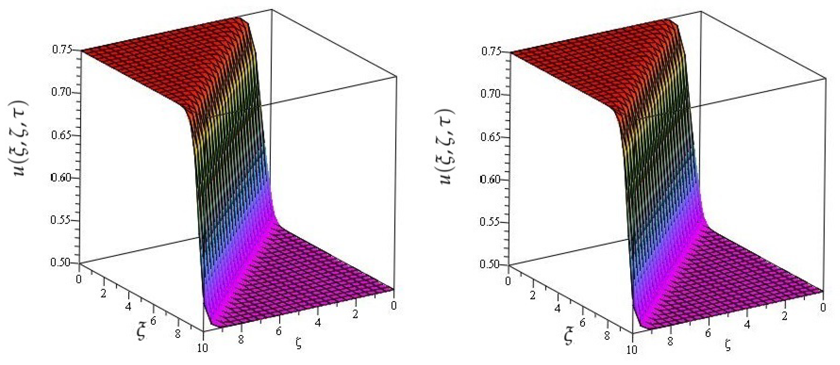
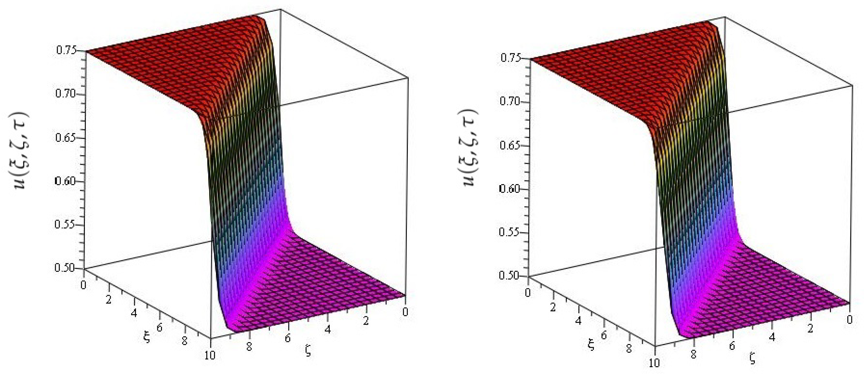
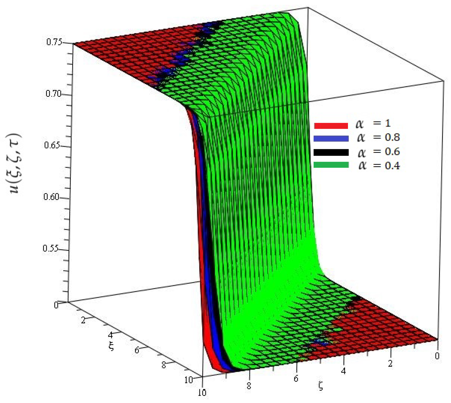
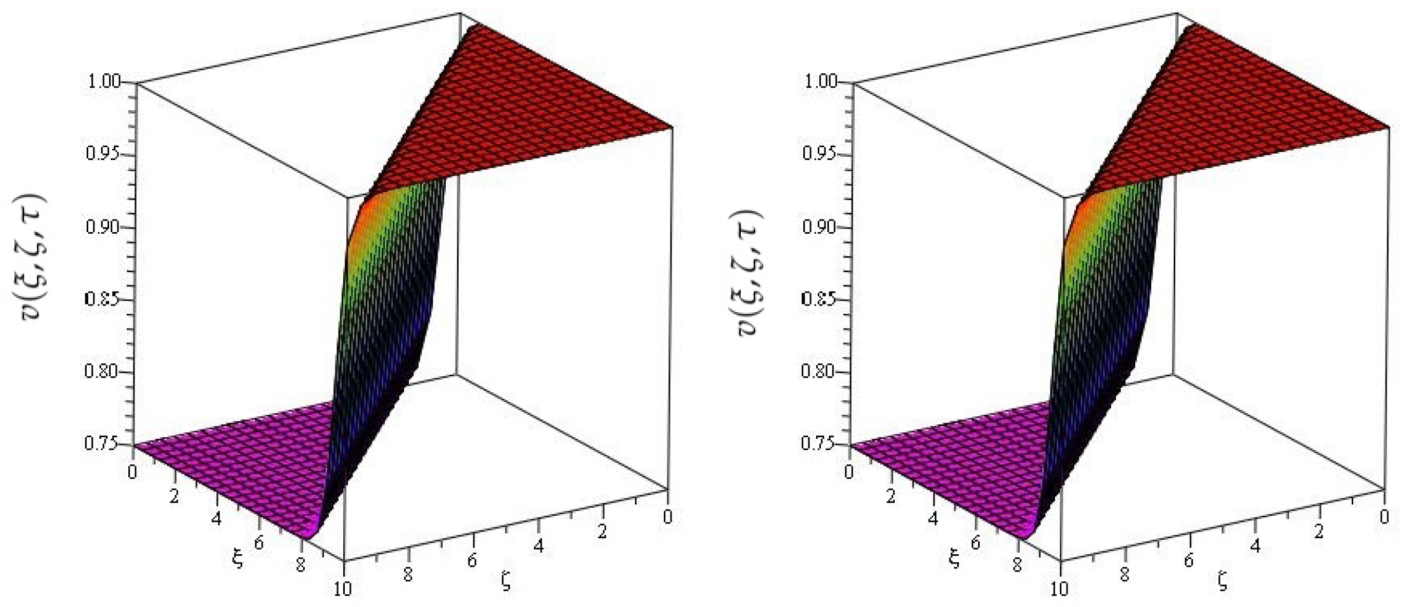
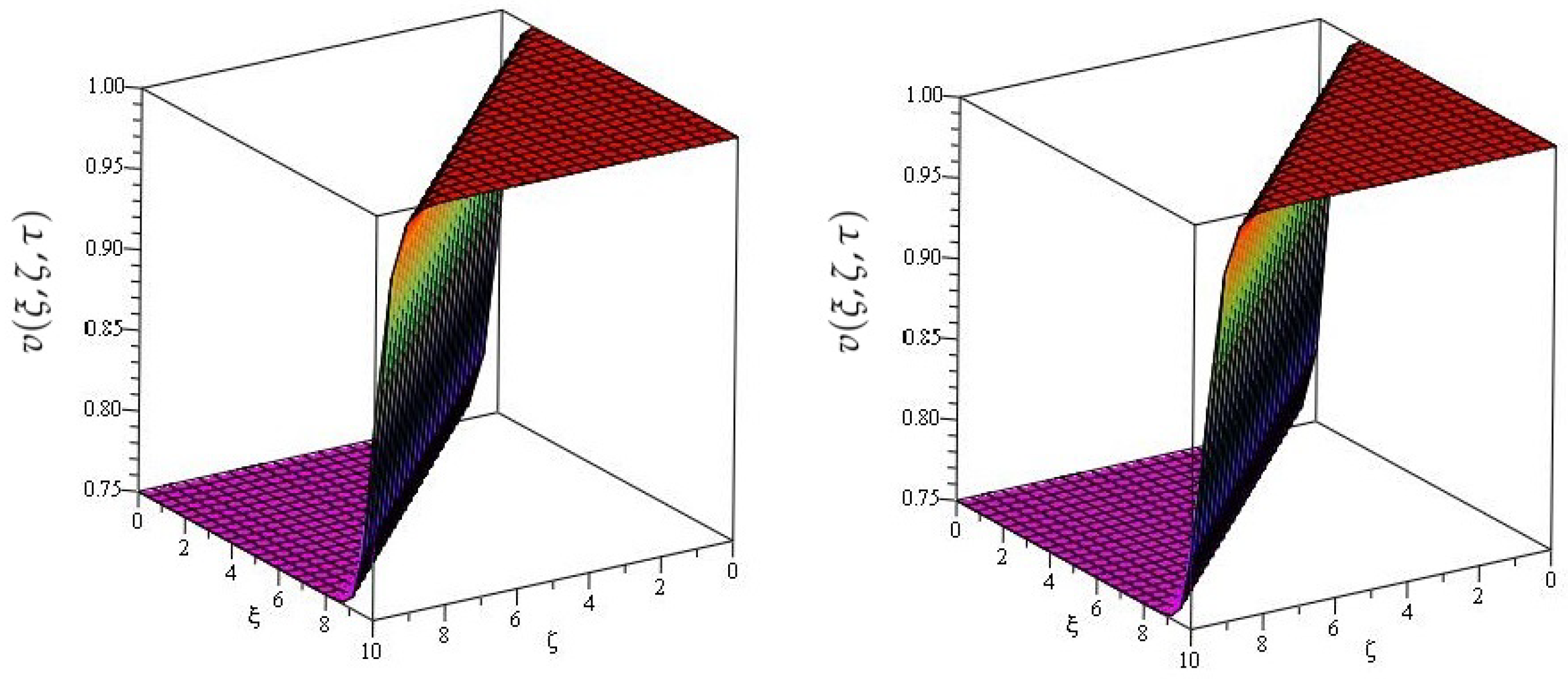
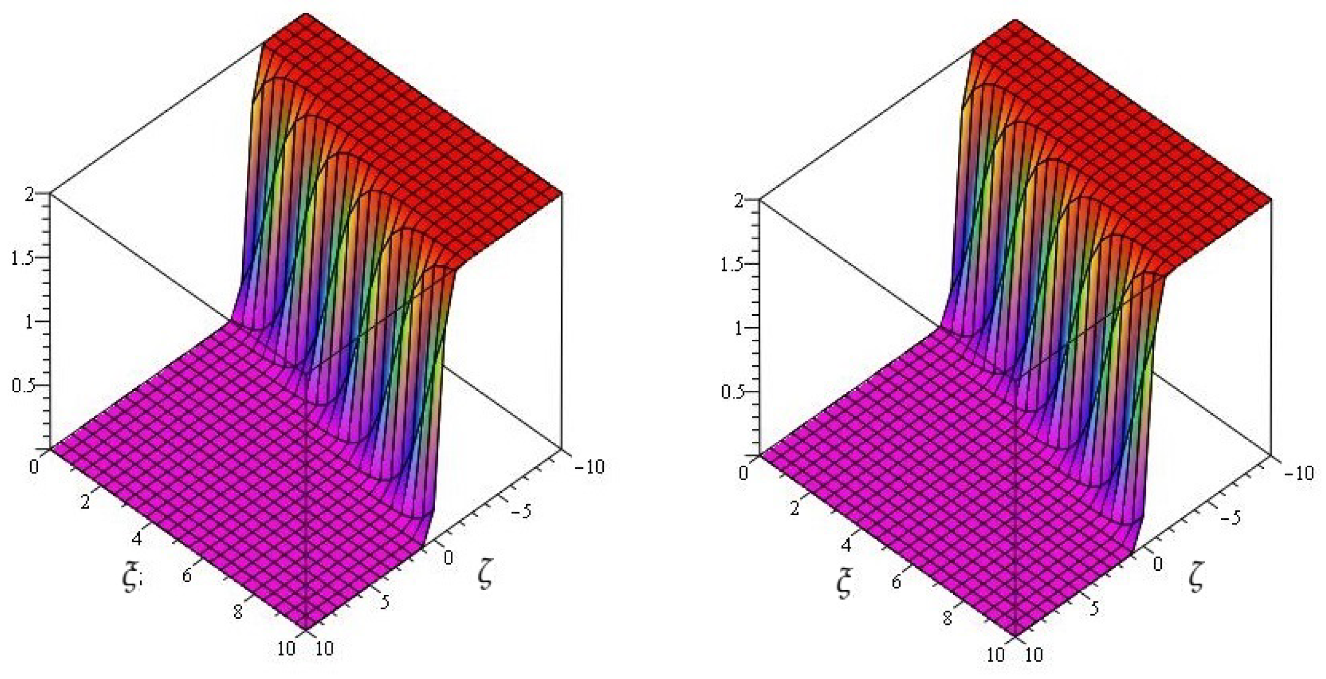
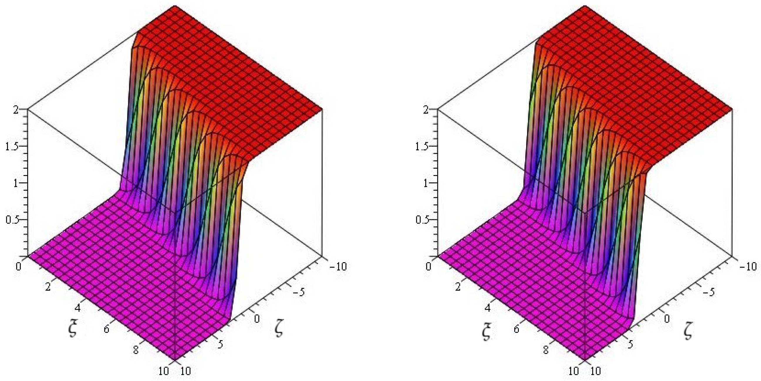
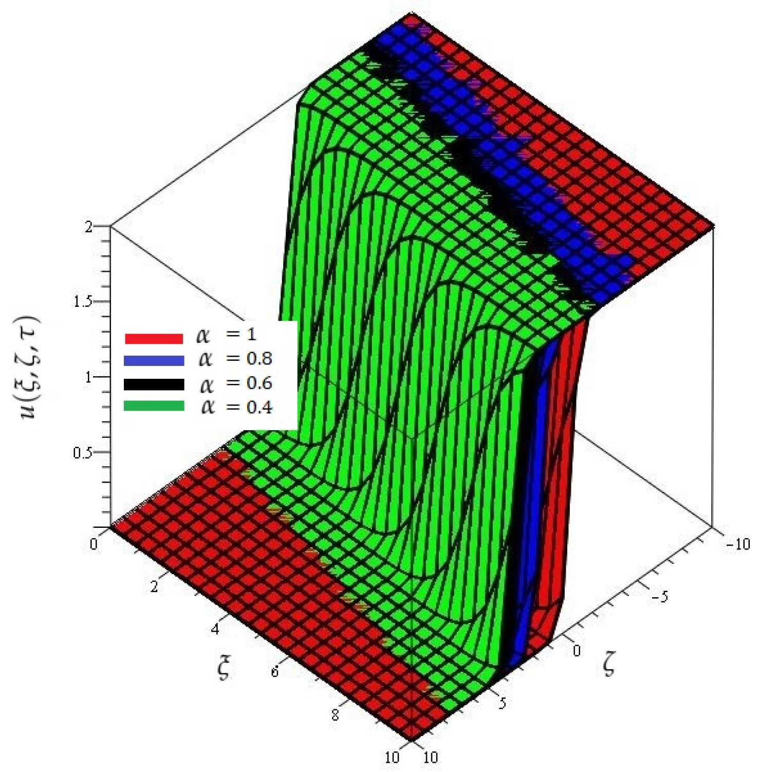
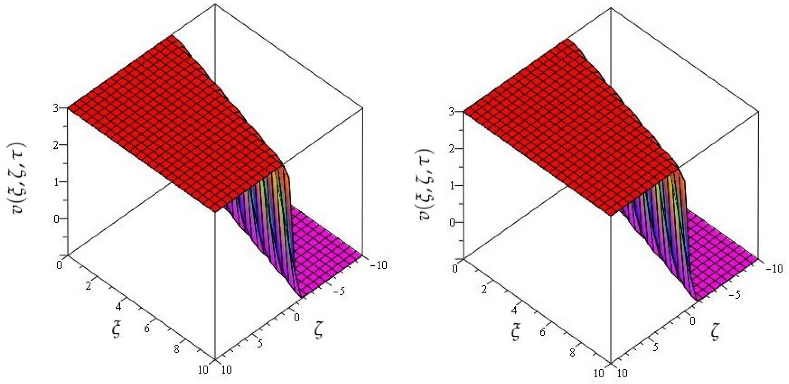
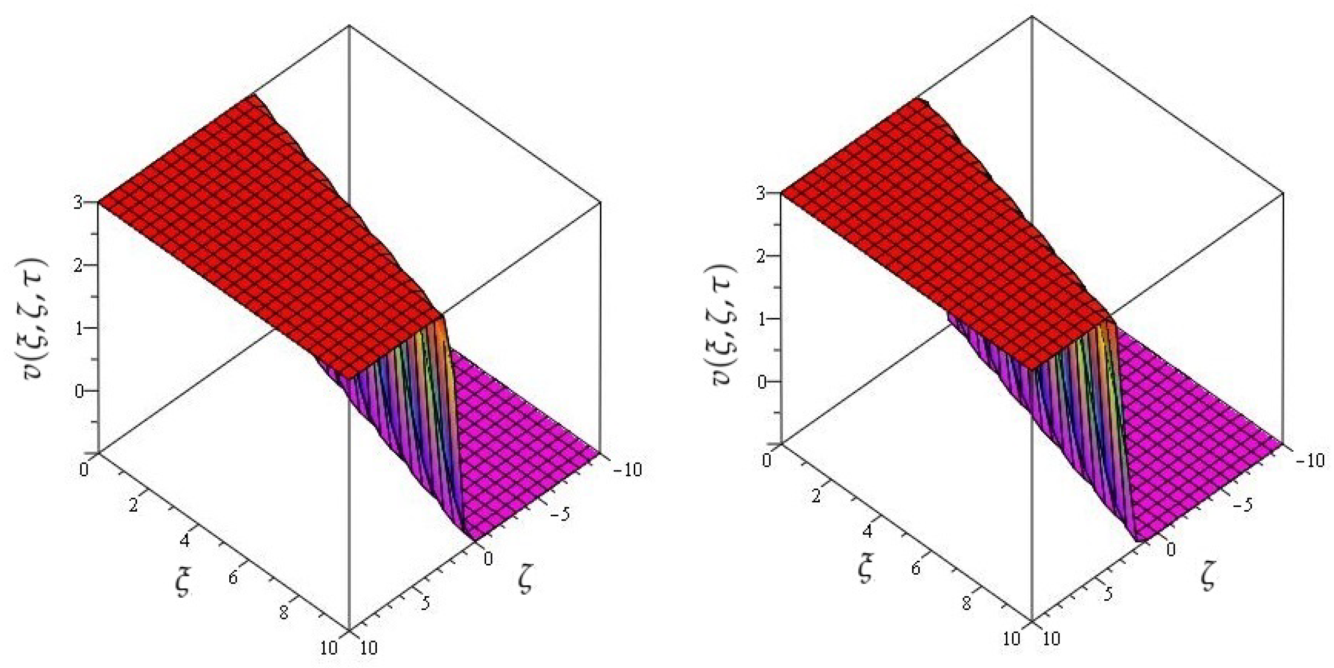
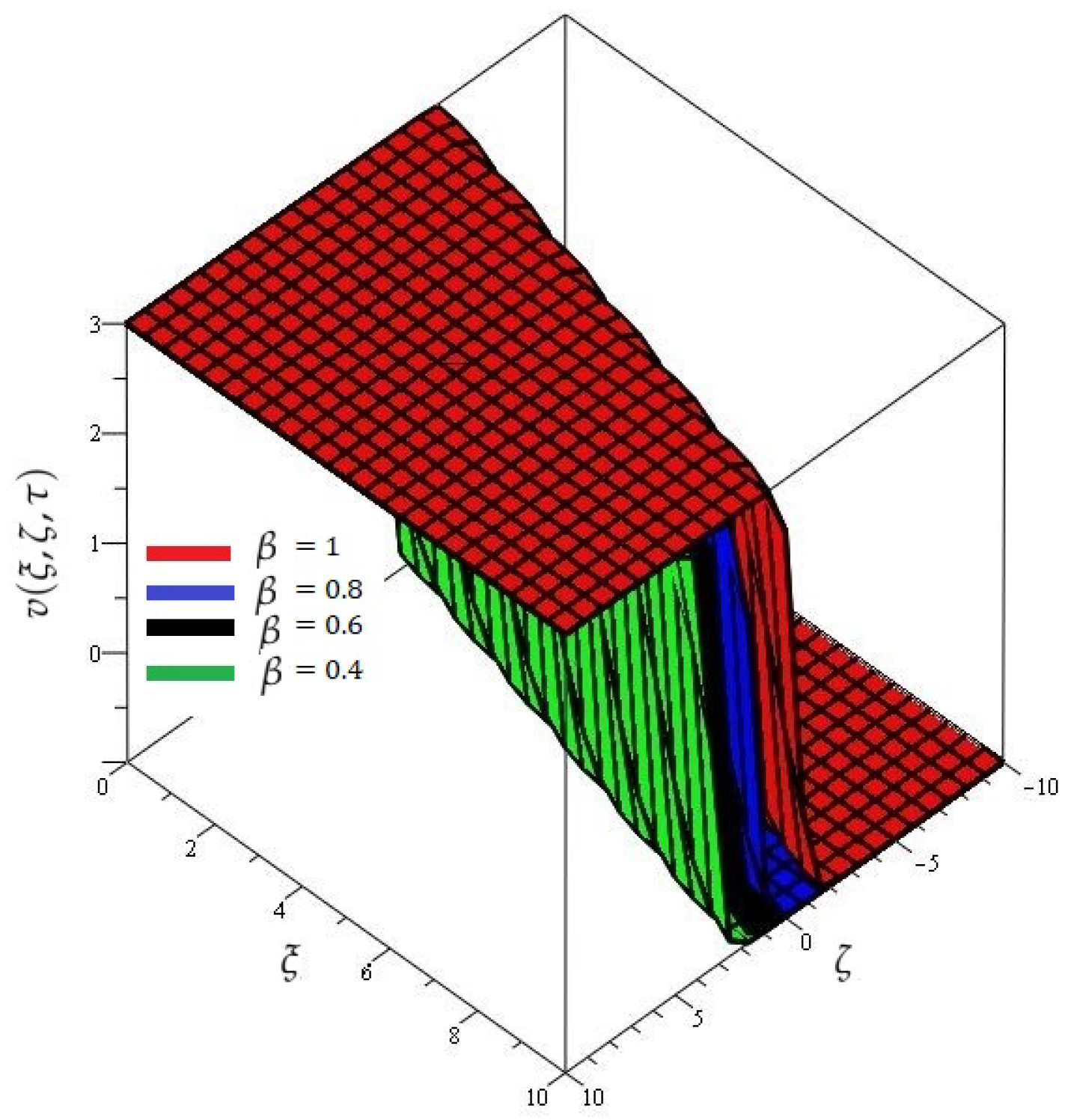
In this study, we have successfully applied two novel methods to investigate the numerical solution of fractional coupled Burgers equations. Find numerical data for the system of Burgers equations at any order for different values of space and time variables with Maple 13. In

Table 1. The exact, $NTD{M}_{CF}$ and $NTD{M}_{ABC}$ solutions of $v(\xi ,\zeta ,\tau )$ for Example 1 at different fractional-order of $\alpha$ and $\beta$ with $l=4$ for different $\xi$ and $\tau$ when $\zeta =1$.

$\mathit{\xi }$	t	$\mathit{\alpha }=\mathit{\beta }=0.6$	$\mathit{\alpha }=\mathit{\beta }=0.75$	$\mathit{\alpha }=\mathit{\beta }=0.9$	$\mathit{\alpha }=\mathit{\beta }=1\left(\mathit{Approx}\right)$	$\mathit{\alpha }=\mathit{\beta }=1\left(\mathit{Exact}\right)$
	0.2	0.760060	0.760035	0.760025	0.760021	0.760021
	0.4	0.760148	0.760081	0.760050	0.760039	0.760040
0.2	0.6	0.760284	0.760158	0.760095	0.760071	0.760074
	0.8	0.760473	0.760278	0.760167	0.760123	0.760138
	1	0.760720	0.760449	0.760278	0.760205	0.760258
	0.2	0.760728	0.760430	0.760304	0.760258	0.760258
	0.4	0.761784	0.760978	0.760610	0.760477	0.760482
0.4	0.6	0.763420	0.761915	0.76149	0.760861	0.760898
	0.8	0.765698	0.763357	0.762026	0.761493	0.761673
	1	0.768663	0.765415	0.763362	0.762482	0.763108
	0.2	0.768374	0.765097	0.763645	0.763104	0.763108
	0.4	0.769658	0.761211	0.767177	0.765676	0.765744
0.6	0.6	0.796654	0.781353	0.763235	0.760073	0.760522
	0.8	0.819877	0.796626	0.782885	0.767192	0.768965
	1	0.849767	0.818099	0.797332	0.788131	0.793241
	0.2	0.821594	0.807747	0.807683	0.793103	0.793241
	0.4	0.848508	0.839515	0.833718	0.804635	0.805676
0.8	0.6	0.857888	0.871744	0.867444	0.844863	0.847161
	0.8	0.844810	0.899765	0.897914	0.884778	0.886000
	1	0.805199	0.918764	0.919533	0.925065	0.912839
	0.2	0.950038	0.944350	0.941824	0.923764	0.922839
	0.4	0.915159	0.958238	0.973309	0.958357	0.954325
1	0.6	0.791894	0.916308	0.977100	0.978048	0.976759
	0.8	0.569588	0.795564	0.931177	0.964956	0.991035
	1	0.238108	0.571732	0.807906	0.894048	0.909478

and

Table 2. Comparative study between varational iteration method (VIM) [34], $ND{M}_{CF}$ and $ND{M}_{ABC}$ for the numerical result $u(\xi ,\zeta ,\tau )$ of Example 1 at $Re=100$, $\zeta =1$, $\alpha =1$, and $\beta =1$ for $l=4$.

$\mathit{\tau }$	$\mathit{\xi }$	$|{\mathit{u}}_{\mathit{Exact}}-{\mathit{u}}_{\mathit{VIM}}|$	$|{\mathit{u}}_{\mathit{Exact}}-{\mathit{u}}_{\mathit{HPTM}}|$	$|{\mathit{u}}_{\mathit{Exact}}-{\mathit{u}}_{\mathit{EDM}}|$
	0.1	3.2300 × ${10}^{-8}$	5.4246 × ${10}^{-10}$	5.4246 × ${10}^{-10}$
	0.2	6.9000 × ${10}^{-8}$	3.4568 × ${10}^{-10}$	3.4568 × ${10}^{-10}$
0.1	0.3	1.6200 × ${10}^{-7}$	2.2468 × ${10}^{-9}$	2.2468 × ${10}^{-9}$
	0.4	5.9700 × ${10}^{-7}$	6.3267 × ${10}^{-9}$	6.3267 × ${10}^{-9}$
	0.5	1.8660 × ${10}^{-6}$	2.1326 × ${10}^{-8}$	2.1326 × ${10}^{-8}$
	0.1	2.4400 × ${10}^{-7}$	4.7421 × ${10}^{-9}$	4.7421 × ${10}^{-9}$
	0.2	8.3100 × ${10}^{-7}$	3.1235 × ${10}^{-8}$	3.1235 × ${10}^{-8}$
0.2	0.3	2.8500 × ${10}^{-6}$	4.5682 × ${10}^{-8}$	4.5682 × ${10}^{-8}$
	0.4	9.7940 × ${10}^{-6}$	3.5223 × ${10}^{-7}$	3.5223 × ${10}^{-7}$
	0.5	3.2012 × ${10}^{-7}$	2.9315 × ${10}^{-7}$	2.9315 × ${10}^{-7}$
	0.1	2.2981 × ${10}^{-6}$	3.2245 × ${10}^{-7}$	3.2245 × ${10}^{-7}$
	0.2	5.4602 × ${10}^{-6}$	4.2659 × ${10}^{-7}$	4.2659 × ${10}^{-7}$
0.3	0.3	2.5432 × ${10}^{-5}$	1.5348 × ${10}^{-6}$	1.5348 × ${10}^{-6}$
	0.4	6.4229 × ${10}^{-4}$	8.2374 × ${10}^{-6}$	8.2374 × ${10}^{-6}$
	0.5	2.8364 × ${10}^{-4}$	4.1975 × ${10}^{-5}$	4.1975 × ${10}^{-5}$
	0.1	5.5428 × ${10}^{-5}$	2.1351 × ${10}^{-6}$	2.1351 × ${10}^{-6}$
	0.2	2.4133 × ${10}^{-5}$	2.6276 × ${10}^{-6}$	2.6276 × ${10}^{-6}$
0.4	0.3	6.3743 × ${10}^{-5}$	2.2334 × ${10}^{-5}$	2.2334 × ${10}^{-5}$
	0.4	2.9070 × ${10}^{-4}$	1.2035 × ${10}^{-5}$	1.2035 × ${10}^{-5}$
	0.5	6.9763 × ${10}^{-4}$	2.2145 × ${10}^{-4}$	2.2145 × ${10}^{-4}$
	0.1	2.2529 × ${10}^{-5}$	2.3223 × ${10}^{-6}$	2.3223 × ${10}^{-6}$
	0.2	4.9868 × ${10}^{-5}$	3.2721 × ${10}^{-5}$	3.2721 × ${10}^{-5}$
0.5	0.3	4.1932 × ${10}^{-4}$	3.0767 × ${10}^{-5}$	3.0767 × ${10}^{-5}$
	0.4	5.5568 × ${10}^{-4}$	2.3742 × ${10}^{-4}$	2.3742 × ${10}^{-4}$
	0.5	2.4350 × ${10}^{-3}$	1.3223 × ${10}^{-3}$	1.3223 × ${10}^{-3}$

, we perform numerical simulations for various Brownian motions with different $\xi$ and $\tau$ values for the system in problem 1. The numerical comparison of variational iteration method, Natural decomposition method in terms of absolute error for Equation (42) is presented in

Table 3. Comparative study between VIM [34], $NTD{M}_{CF}$ and $NTD{M}_{ABC}$ for the approximate solution $v(\xi ,\zeta ,\tau )$ of Example 1 at $Re=100$, $\zeta =1$, $\alpha =1$, and $\beta =1$ for $l=4$.

$\mathit{\tau }$	$\mathit{\xi }$	$|{\mathit{v}}_{\mathit{Exact}}-{\mathit{v}}_{\mathit{VIM}}|$	$|{\mathit{v}}_{\mathit{Exact}}-{\mathit{v}}_{{\mathit{NTDM}}_{\mathit{CF}}}|$	$|{\mathit{v}}_{\mathit{Exact}}-{\mathit{v}}_{{\mathit{NTDM}}_{\mathit{ABC}}}|$
	0.1	9.0202 × ${10}^{-9}$	1.3770 × ${10}^{-11}$	8.6253 × ${10}^{-11}$
	0.2	5.4060 × ${10}^{-9}$	4.8036 × ${10}^{-10}$	3.1054 × ${10}^{-10}$
0.1	0.3	2.7960 × ${10}^{-8}$	1.6734 × ${10}^{-9}$	1.1992 × ${10}^{-9}$
	0.4	6.5902 × ${10}^{-8}$	5.8013 × ${10}^{-9}$	5.5827 × ${10}^{-9}$
	0.5	3.9762 × ${10}^{-7}$	1.9773 × ${10}^{-8}$	3.6150 × ${10}^{-8}$
	0.1	3.3610 × ${10}^{-8}$	2.3548 × ${10}^{-9}$	2.8894 × ${10}^{-9}$
	0.2	9.1810 × ${10}^{-8}$	8.2143 × ${10}^{-8}$	1.0171 × ${10}^{-8}$
0.2	0.3	1.9482 × ${10}^{-7}$	2.8611 × ${10}^{-8}$	3.6538 × ${10}^{-8}$
	0.4	9.8750 × ${10}^{-7}$	9.2053 × ${10}^{-7}$	1.4010 × ${10}^{-7}$
	0.5	4.2127 × ${10}^{-6}$	3.3727 × ${10}^{-7}$	6.3855 × ${10}^{-7}$
	0.1	2.3872 × ${10}^{-7}$	1.2779 × ${10}^{-8}$	2.3189 × ${10}^{-8}$
	0.2	5.3523 × ${10}^{-7}$	4.4573 × ${10}^{-8}$	8.1227 × ${10}^{-8}$
0.3	0.3	2.5565 × ${10}^{-6}$	1.5522 × ${10}^{-7}$	2.8704 × ${10}^{-7}$
	0.4	6.3787 × ${10}^{-6}$	5.3749 × ${10}^{-6}$	1.0445 × ${10}^{-6}$
	0.5	2.8365 × ${10}^{-5}$	1.8244 × ${10}^{-6}$	4.1512 × ${10}^{-6}$
	0.1	5.2272 × ${10}^{-6}$	4.3423 × ${10}^{-7}$	1.0363 × ${10}^{-7}$
	0.2	2.6215 × ${10}^{-6}$	1.5145 × ${10}^{-7}$	3.6229 × ${10}^{-7}$
0.4	0.3	6.3642 × ${10}^{-6}$	5.2723 × ${10}^{-6}$	1.2717 × ${10}^{-6}$
	0.4	2.9203 × ${10}^{-5}$	1.8244 × ${10}^{-6}$	4.5250 × ${10}^{-6}$
	0.5	6.9958 × ${10}^{-5}$	6.1751 × ${10}^{-5}$	1.6814 × ${10}^{-5}$
	0.1	2.2532 × ${10}^{-6}$	1.1434 × ${10}^{-7}$	3.3630 × ${10}^{-7}$
	0.2	4.8935 × ${10}^{-6}$	3.9879 × ${10}^{-6}$	1.1745 × ${10}^{-6}$
0.5	0.3	2.4921 × ${10}^{-5}$	1.3880 × ${10}^{-6}$	4.1074 × ${10}^{-6}$
	0.4	5.8486 × ${10}^{-5}$	4.7977 × ${10}^{-5}$	1.4434 × ${10}^{-5}$
	0.5	1.6542 × ${10}^{-4}$	1.6182 × ${10}^{-5}$	5.1527 × ${10}^{-5}$

and

Table 4. The exact, $NTD{M}_{CF}$ and $NTD{M}_{ABC}$ solutions of $u(\xi ,\zeta ,\tau )$ for Example 2 at different fractional-order of $\alpha$ and $\beta$ with $l=4$ for different $\xi$ and $\tau$ when $\zeta =1$.

$\mathit{\xi }$	$\mathit{\tau }$	$\mathit{\alpha }=\mathit{\beta }=0.6$	$\mathit{\alpha }=\mathit{\beta }=0.75$	$\mathit{\alpha }=\mathit{\beta }=0.9$	$\mathit{\alpha }=\mathit{\beta }=1\left(\mathit{Approx}\right)$	$\mathit{\alpha }=\mathit{\beta }=1\left(\mathit{Exact}\right)$
	0.2	0.007531	0.003305	0.003056	0.003355	0.003318
	0.4	0.037374	0.010555	0.003583	0.002299	0.001492
0.2	0.6	0.107634	0.037076	0.011908	0.005587	0.000671
	0.8	0.228832	0.095214	0.035864	0.017981	0.000301
	1	0.409637	0.198269	0.086536	0.047619	0.000135
	0.2	0.010890	0.004952	0.004581	0.005015	0.004945
	0.4	0.054113	0.015998	0.005662	0.003639	0.002225
0.4	0.6	0.156343	0.056189	0.019107	0.009354	0.001000
	0.8	0.333035	0.144112	0.057207	0.029946	0.000450
	1	0.596925	0.299764	0.137217	0.078479	0.000202
	0.2	0.015625	0.007446	0.006882	0.007503	0.007368
	0.4	0.077841	0.024529	0.009141	0.005878	0.003318
0.6	0.6	0.225856	0.086120	0.031439	0.016138	0.001492
	0.8	0.482298	0.220396	0.093435	0.051355	0.000671
	1	0.865819	0.457619	0.222442	0.132987	0.000301
	0.2	0.022393	0.011281	0.010372	0.011236	0.010973
	0.4	0.112097	0.038380	0.015138	0.009711	0.004945
0.8	0.6	0.326798	0.134623	0.053250	0.028657	0.002225
	0.8	0.699653	0.343269	0.156889	0.090621	0.001000
	1	1.257990	0.710643	0.370200	0.231727	0.000450
	0.2	0.032749	0.017333	0.015694	0.016848	0.016325
	0.4	0.165420	0.062144	0.025783	0.016410	0.007368
1	0.6	0.483746	0.217538	0.092962	0.052080	0.003318
	0.8	1.036890	0.551429	0.271315	0.163669	0.001492
	1	1.865360	1.136210	0.633917	0.413380	0.000670

.

Table 5. The exact, $NTD{M}_{CF}$ and $NTD{M}_{ABC}$ solutions of $v(\xi ,\zeta ,\tau )$ for Example 2 at different fractional-order of $\alpha$ and $\beta$ with $l=4$ for different $\xi$ and $\tau$ when $\zeta =1$.

$\mathit{\xi }$	$\mathit{\tau }$	$\mathit{\alpha }=\mathit{\beta }=0.6$	$\mathit{\alpha }=\mathit{\beta }=0.75$	$\mathit{\alpha }=\mathit{\beta }=0.9$	$\mathit{\alpha }=\mathit{\beta }=1\left(\mathit{Approx}\right)$	$\mathit{\alpha }=\mathit{\beta }=1\left(\mathit{Exact}\right)$
	0.2	3.010560	2.998480	2.994809	2.993571	2.993365
	0.4	3.060490	3.019625	3.003995	2.999902	2.997016
0.2	0.6	3.142602	3.063333	3.024227	3.011611	2.998659
	0.8	3.256140	3.135462	3.063606	3.036047	2.999397
	1	3.400174	3.239966	3.129121	3.080563	2.999729
	0.2	3.015831	2.997739	2.992253	2.990409	2.990109
	0.4	3.090282	3.029146	3.005834	2.999757	2.995550
0.4	0.6	3.212598	3.093978	3.035646	3.016907	2.998000
	0.8	3.381655	3.200917	3.093647	3.052668	2.999101
	1	3.596061	3.355824	3.190150	3.117848	2.999596
	0.2	3.023772	2.996638	2.988438	2.985692	2.985263
	0.4	3.134729	3.043180	3.008425	2.999423	2.993365
0.6	0.6	3.316769	3.139066	3.052084	3.024316	2.997016
	0.8	3.568204	3.297118	3.136975	3.076147	2.998659
	1	3.886965	3.525992	3.278240	3.170692	2.999397
	0.2	3.035766	2.995000	2.982740	2.978658	2.978054
	0.4	3.200960	3.063729	3.011961	2.998675	2.990109
0.8	0.6	3.471437	3.204907	3.075310	3.034312	2.995550
	0.8	3.844671	3.437381	3.198374	3.108342	2.997999
	1	4.317582	3.773870	3.403204	3.243539	2.999101
	0.2	3.053892	2.992555	2.974226	2.968170	2.967350
	0.4	3.299308	3.093483	3.016524	2.997036	2.985263
1	0.6	3.699990	3.299910	3.107172	3.046991	2.993365
	0.8	4.252157	3.639306	3.283009	3.150375	2.997015
	1	4.951244	4.130244	3.575765	3.339528	2.998659

and

Table 6. Comparative study between VIM, $NTD{M}_{CF}$ and $NTD{M}_{ABC}$ for the approximate solution $u(\xi ,\zeta ,\tau )$ of Example 2 at $Re=100$, $\zeta =0.3$, $\alpha =1$, and $\beta =1$ for $n=4$.

$\mathit{\tau }$	$\mathit{\xi }$	$|{\mathit{u}}_{\mathit{Exact}}-{\mathit{u}}_{\mathit{VIM}}|$	$|{\mathit{u}}_{\mathit{Exact}}-{\mathit{u}}_{{\mathit{NTDM}}_{\mathit{CF}}}|$	$|{\mathit{u}}_{\mathit{Exact}}-{\mathit{u}}_{{\mathit{NTDM}}_{\mathit{ABC}}}|$
	0.1	0.00388488	0.000040388	0.0000403885
	0.2	0.02058640	0.000643080	0.0006430800
0.1	0.3	0.08300040	0.003204730	0.0032047300
	0.4	0.19216900	0.009896630	0.0098966300
	0.5	0.35630400	0.023490500	0.0234905000
	0.1	0.00340343	0.000037786	0.0000377862
	0.2	0.02549380	0.000619573	0.0006195730
0.2	0.3	0.09466810	0.003156030	0.0031560300
	0.4	0.21124200	0.009911520	0.0099115200
	0.5	0.38165100	0.023838100	0.0238381000
	0.1	0.00290734	0.000030901	0.0000309013
	0.2	0.02730130	0.000536002	0.0005360020
0.3	0.3	0.09244390	0.002840270	0.0028402700
	0.4	0.19342500	0.009181990	0.0091819900
	0.5	0.33037500	0.022574100	0.0225741000
	0.1	0.00271456	0.000018180	0.0000181808
	0.2	0.02207170	0.000368845	0.0003688450
0.4	0.3	0.06204090	0.002146160	0.0021461600
	0.4	0.10393800	0.007381420	0.0073814200
	0.5	0.13365400	0.018959600	0.0189596000
	0.1	0.00334970	1.950740 × ${10}^{-6}$	1.9507400 × ${10}^{-6}$
	0.2	0.00408341	0.000093131	0.0000931316
0.5	0.3	0.01675610	0.000951695	0.0009516950
	0.4	0.10582700	0.004143110	0.0041431100
	0.5	0.30400000	0.012150100	0.0121501000

show the results of a numerical study for the coupled system considered in problem 2. Analogously, in

Table 7. Comparative study between VIM [34], $NTD{M}_{CF}$ and $NTD{M}_{ABC}$ for the approximate solution $v(\xi ,\zeta ,\tau )$ of Example 2 at $Re=100$, $\zeta =0.3$, $\alpha =1$, and $\beta =1$ for $l=4$.

$\mathit{\tau }$	$\mathit{\xi }$	$|{\mathit{v}}_{\mathit{Exact}}-{\mathit{v}}_{\mathit{VIM}}|$	$|{\mathit{v}}_{\mathit{Exact}}-{\mathit{v}}_{{\mathit{NTDM}}_{\mathit{CF}}}|$	$|{\mathit{v}}_{\mathit{Exact}}-{\mathit{v}}_{{\mathit{NTDM}}_{\mathit{ABC}}}|$
	0.1	0.000409157	0.000080777	0.000080777
	0.2	0.00179639	0.00128616	0.00128616
0.1	0.3	0.00575008	0.00640947	0.00640947
	0.4	0.0154079	0.0197933	0.0197933
	0.5	0.0351083	0.046981	0.046981
	0.1	0.000358137	0.0000755724	0.0000755724
	0.2	0.000618968	0.00123915	0.00123915
0.2	0.3	0.00097818	0.00631207	0.00631207
	0.4	0.00333882	0.019823	0.019823
	0.5	0.0109793	0.0476761	0.0476761
	0.1	0.000169508	0.0000618027	0.0000618027
	0.2	0.00190188	0.001072	0.001072
0.3	0.3	0.0086713	0.00568053	0.00568053
	0.4	0.0207692	0.018364	0.018364
	0.5	0.0372769	0.0451482	0.0451482
	0.1	0.000255194	0.0000363616	0.0000363616
	0.2	0.00656152	0.00073769	0.00073769
0.4	0.3	0.0259301	0.00429232	0.00429232
	0.4	0.0634979	0.0147628	0.0147628
	0.5	0.122694	0.0379192	0.0379192
	0.1	0.00104781	3.90148 × ${10}^{-6}$	3.90148 × ${10}^{-6}$
	0.2	0.0143686	0.000186263	0.000186263
0.5	0.3	0.0541981	0.00190339	0.00190339
	0.4	0.132966	0.00828621	0.00828621
	0.5	0.261277	0.0243001	0.0243001

, we compare the solution to Equation (61) obtained by variational iteration method, Natural decomposition method. Based on the data in the tables above, we can conclude that the results achieved by the Natural decomposition method are more reliable. The behavior of the Natural decomposition method result from $u(\xi ,\zeta ,\tau )$ for problem 1 is represented in Figure 1, and the nature of the actual result and different fractional-order of $\alpha$ are provided in Figure 2, respectively. In Figure 3 show that the different fractional-order at $\alpha =1,0.8,0.6$ and $0.4$. In the same way, the achieved result $v(\xi ,\zeta ,\tau )$ for Equation (61) can be seen in Figure 4. Figure 5 and Figure 6 are the response of acquired results for problem 1 with different standard motion and Brownian motions $\beta =0.8$ and $0.6$. The behavior of the Natural decomposition method result from $u(\xi ,\zeta ,\tau )$ for problem 2 is represented in Figure 7, and the nature of the actual result and different fractional-order of $\alpha$ are provided in Figure 8, respectively. In Figure 9 show that the different fractional-order at $\alpha =1,0.8,0.6$ and $0.4$. In the same way, the achieved result $v(\xi ,\zeta ,\tau )$ for Equation (61) can be seen in Figure 10. Figure 11 and Figure 12 are the response of acquired results for problem 1 with different standard motion and Brownian motion $\beta =0.8$ and $0.6$.

6. Conclusions

In the present article, Natural decomposition method is applied for the solution of coupled systems of fractional Burger equations. The graphical and tabular representations of the derived results have been done. The solutions are obtained for fractional systems which are closely related to their actual solutions. The suggested technique provides a series result in a form of recurrence relation with high accuracy and minimal calculations. Numerous computational results are compared with well-known numerical techniques and the exact results when $\alpha =\beta =1$. These representation of the obtained results have clearly confirmed the higher accuracy of the suggested methods. The convergence of fractional solutions to integer order solution have been shown. The less calculations and higher accuracy are the valuable themes of the present methods. The researchers are then modified it to solve other systems with fractional partial differential equations.

References

- Hilfer, R. Applications of Fractional Calculus in Physics; World Scientific Publishing Co., Inc.: River Edge, NJ, USA, 2000. [Google Scholar]
- Kilbas, A.A.; Srivastava, H.M.; Trujillo, J.J. Theory and Applications of Fractional Differential Equations; North Holland Mathematics Studies, Elsevier Science B.V.: Amsterdam, The Netherlands, 2006. [Google Scholar]
- Baleanu, D.; Diethelm, K.; Scalas, E.; Trujillo, J.J. Fractional Calculus, Series on Complexity, Nonlinearity and Chaos; World Scientific Publishing Co. Pte. Ltd.: Hackensack, NJ, USA, 2012; Volume 3. [Google Scholar]
- Srivastava, H.M.; Kumar, D.; Singh, J. An efficient analytical technique for fractional model of vibration equation. Appl. Math. Model. 2017, 45, 192–204. [Google Scholar] [CrossRef]
- Imtiaz, A.; Foong, O.M.; Aamina, A.; Khan, N.; Ali, F.; Khan, I. Generalized Model of Blood Flow in a Vertical Tube with Suspension of Gold Nanomaterials: Applications in the Cancer Therapy. CMC-Comput. Mater. Contin. 2020, 65, 171–192. [Google Scholar] [CrossRef]
- Aljahdaly, N.H. New application through multistage differential transform method. AIP Conf. Proc. 2020, 2293, 420025. [Google Scholar]
- Aljahdaly, N.H.; El-Tantawy, S.A. On the multistage differential transformation method for analyzing damping Duffing oscillator and its applications to plasma physics. Mathematics 2021, 9, 432. [Google Scholar] [CrossRef]
- Wu, G.C.; Baleanu, D. Variational iteration method for fractional calculus-a universal approach by Laplace transform. Adv. Differ. Equations 2013, 2013, 18. [Google Scholar] [CrossRef] [Green Version]
- Khader, M.M.; Kumar, S.; Abbasbandy, S. New homotopy analysis transform method for solving the discontinued problems arising in nanotechnology. Chin. Phys. B 2013, 22, 110201. [Google Scholar] [CrossRef]
- Jleli, M.; Kumar, S.; Kumar, R.; Samet, B. Analytical approach for time fractional wave equations in the sense of Yang-Abdel-Aty-Cattani via the homotopy perturbation transform method. Alex. Eng. J. 2020, 59, 2859–2863. [Google Scholar] [CrossRef]
- Prakash, A.; Goyal, M.; Gupta, S. q-homotopy analysis method for fractional Bloch model arising in nuclear magnetic resonance via the Laplace transform. Indian J. Phys. 2020, 94, 507–520. [Google Scholar] [CrossRef]
- Sunthrayuth, P.; Shah, R.; Zidan, A.M.; Khan, S.; Kafle, J. The Analysis of Fractional-Order Navier-Stokes Model Arising in the Unsteady Flow of a Viscous Fluid via Shehu Transform. J. Funct. Spaces 2021, 2021, 1029196. [Google Scholar]
- Mirzaee, F.; Samadyar, N. On the numerical solution of stochastic quadratic integral equations via operational matrix method. Math. Methods Appl. Sci. 2018, 41, 4465–4479. [Google Scholar] [CrossRef]
- Shah, R.; Khan, H.; Baleanu, D. Fractional Whitham-Broer-Kaup equations within modified analytical approaches. Axioms 2019, 8, 125. [Google Scholar] [CrossRef] [Green Version]
- Sohail, A.; Maqbool, K.; Ellahi, R. Stability analysis for fractional-order partial differential equations by means of space spectral time Adams Bashforth Moulton method. Numer. Methods Partial. Differ. Equ. 2018, 34, 19–29. [Google Scholar] [CrossRef]
- Burgers, J.M. Hydrodynamics-Application of a model system to illustrate some points of the statistical theory of free turbulence. In Selected Papers of JM Burgers; Springer: Dordrecht, The Netherlands, 1995; pp. 390–400. [Google Scholar]
- Aksan, E.N. Quadratic B-spline finite element method for numerical solution of the Burgers equation. Appl. Math. Comput. 2006, 174, 884–896. [Google Scholar] [CrossRef]
- Kutluay, S.; Esen, A. A lumped Galerkin method for solving the Burgers equation. Int. J. Comput. Math. 2004, 81, 1433–1444. [Google Scholar] [CrossRef]
- Abbasbandy, S.; Darvishi, M.T. A numerical solution of Burgers equation by modified Adomian method. Appl. Math. Comput. 2005, 163, 1265–1272. [Google Scholar] [CrossRef]
- Zuo, J.-M.; Zhang, Y.-M.; Abd AL-Hussein, W.R.; Mahmood, A.; Shamran, S.N.K. Exact solutions of the two-dimensional Burgers equation. J. Phys. A Math. Gen. 1999, 32, 6897–6900. [Google Scholar]
- Bateman, H. Some recent researches on the motion of fluids. Mon. Weather. Rev. 1915, 43, 163–170. [Google Scholar] [CrossRef]
- Hopf, E. The partial differential equation ut + uux = uxx. Commun. Pure Appl. Math. 1950, 3, 201–230. [Google Scholar] [CrossRef]
- Cole, J.D. On a quasi-linear parabolic equation occurring in aerodynamics. Q. Appl. Math. 1951, 9, 225–236. [Google Scholar] [CrossRef] [Green Version]
- Benton, E.R.; Platzman, G.W. A table of solutions of the one-dimensional Burgers equation. Q. Appl. Math. 1972, 30, 195–212. [Google Scholar] [CrossRef] [Green Version]
- Karpman, V.I. Non-Linear Waves in Dispersive Media: International Series of Monographs in Natural Philosophy; Elsevier: Amsterdam, The Netherlands, 2016; Volume 71. [Google Scholar]
- Rawashdeh, M.; Maitama, S. Finding exact solutions of nonlinear PDEs using the natural decomposition method. Math. Methods Appl. Sci. 2017, 40, 223–236. [Google Scholar] [CrossRef]
- Veeresha, P.; Prakasha, D.G.; Baskonus, H.M. Novel simulations to the time-fractional Fishers equation. Math. Sci. 2019, 13, 33–42. [Google Scholar] [CrossRef]
- Miller, K.S.; Ross, B. An Introduction to the Fractional Calculus and Fractional Differential Equations; A Wiley Spaces Inter Science Publication; John Wiley & Sons, Inc.: New York, NY, USA, 1993. [Google Scholar]
- Podlubny, I. Fractional Differential Equations, in Mathematics in Science and Engineering; Academic Press, Inc.: San Diego, CA, USA, 1999; p. 198. [Google Scholar]
- Diethelm, K. The Analysis of Fractional Differential Equations; Lecture Notes in Mathematics; Springer: Berlin/Heidelberg, Germany, 2010. [Google Scholar]
- Zhou, M.X.; Kanth, A.S.V.; Aruna, K.; Raghavendar, K.; Rezazadeh, H.; Mustafa Inc.; Aly, A.A. Numerical Solutions of Time Fractional Zakharov-Kuznetsov Equation via Natural Transform Decomposition Method with Nonsingular Kernel Derivatives. J. Funct. Spaces 2021, 2021, 9884027. [Google Scholar]
- Adomian, G. A new approach to nonlinear partial differential equations. J. Math. Anal. Appl. 1984, 102, 420–434. [Google Scholar] [CrossRef] [Green Version]
- Adomian, G. Solving Frontier Problems of Physics: The Decomposition Method; With a Preface by Yves Cherruault. Fundamental Theories of Physics; Kluwer Academic Publishers Group: Dordrecht, The Netherlands, 1994. [Google Scholar]
- Soliman, A.A. On the solution of two-dimensional coupled Burgers equations by variational iteration method. Chaos Solitons Fractals 2009, 40, 1146–1155. [Google Scholar] [CrossRef]
Figure 1.
The exact and numerical solutions of of Example 1 at .
Figure 2.
The numerical solution graph of of Example 1 at and .
Figure 3.
The numerical solution graph of of Example 1 at different value of .
Figure 4.
Figure 5.
Figure 6.
Figure 7.
The exact and numerical solutions of of Example 2 at .
Figure 8.
The numerical solution graph of of Example 2 at and .
Figure 9.
The numerical solution graph of of Example 2 at different value of .
Figure 10.
Figure 11.
Figure 12.