2.1 Data

This study employs the model output from the Precipitation Driver and Response Model Intercomparison Project (PDRMIP), utilizing simulations examining the climate responses to individual climate drivers (Myhre et al., 2017). The eight models used in this study are CanESM2, GISS-E2R, HadGEM2-ES, HadGEM3, MIROC, CESM-CAM4, CESM-CAM5, and NorESM. The versions of these models are essentially the same as their versions in the 5th Assessment Report of the Intergovernmental Panel on Climate Change (IPCC AR5). The configurations and basic settings are listed in Table 1. In these simulations, five separate perturbations were applied to all the models instantly on a global scale: a doubling of CO₂ concentration (CO₂×2), a tripling of CH₄ concentration (CH₄×3), a 2 % increase in solar irradiance (solar + 2 %), a 10-fold increase in present-day black carbon concentration/emission (BC × 10), and a 5-fold increase in present-day SO₄ concentration/emission (SO₄×5). Each perturbation was run in two parallel configurations, a 15-year fixed sea surface temperature (fsst) simulation and a 100-year coupled simulation. The former is compared with its fsst control simulation to diagnose the ERF at the TOA and fast responses in each model, whereas the latter is used to examine climate responses. One model (CESM-CAM4) used a slab ocean setup for the coupled simulation whereas the others used a full dynamic ocean. For aerosol perturbations, monthly year 2000 concentrations were derived from the AeroCom Phase II initiative (Myhre et al., 2013a) and multiplied by the stated factors in concentration-driven models. Some models were unable to perform simulations with prescribed concentrations. These models multiplied emissions by these factors instead (Table 1). The aerosol loadings in the NorESM model for the two aerosol perturbations are shown in Fig. 1 for an illustrative purpose; the spatial patterns are similar for other models. In the BC experiment, the concentration is highest in east China (E. China), followed by India, tropical Africa and South America (S. America). In the current study, these four regions are referred to as source regions due to their high emissions while the US and Europe are defined as non-source regions due to their relatively low emissions. For the SO₄ experiment, the aerosols are mainly restricted to the Northern Hemisphere (NH), with the highest loading observed in E. China, followed by India and Europe. The eastern US also has moderately high concentrations. More detailed descriptions of PDRMIP and some PDRMIP findings are given in Samset et al. (2016), Myhre et al. (2017), and Tang et al. (2018).

Table 1Descriptions of the eight PDRMIP models used in this study.

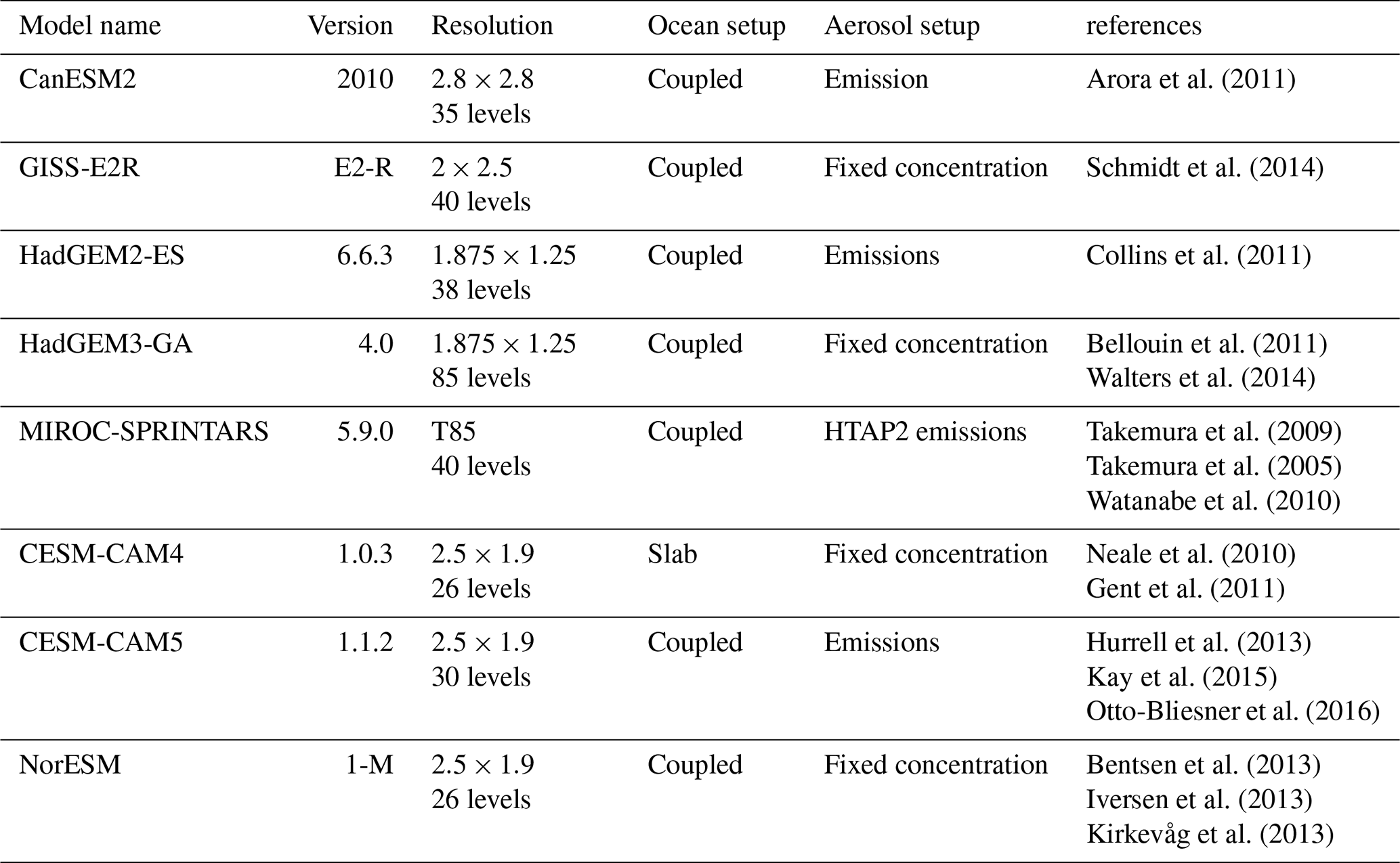
Note: HTAP2 is Hemispheric Transport Air Pollution, Phase 2.

Download Print Version | Download XLSX

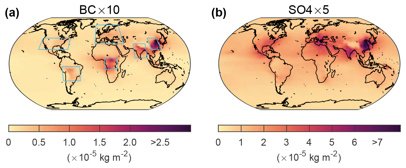
Figure 1Aerosol loadings for the two aerosol experiments in the NorESM model.

2.2 Methods

In this study, we start from the surface energy balance. We restrict our discussions to land grids only because this is where most people live, and thus the temperature response over land is more important to the well-being of humans. The incoming radiative energy (R_in) includes

In Eq. (1), ↓SW represents downward shortwave radiation and ↑SW represents reflected SW radiation. ↓LW denotes the downward LW radiation. The law of energy conservation requires that the R_in should be balanced by the outgoing energy (E_out):

In Eq. (2), ↑LW is the outgoing longwave radiation, which is a function of temperature based on the Stefan–Boltzmann law. H, λE, and G denote sensible heat flux, latent heat flux, and ground heat flux, respectively. For latent heat flux (λE), λ is the specific latent heat of evaporation, and E is the evaporation rate. R_in is defined as surface radiative heating, as it is the radiative input provided to the surface to raise the surface temperature (Wild et al., 2004). The surface responds to the imposed energy by redistributing the energy content through each E_out component. Since R_in is equal to E_out, we have

The changes of each energy component, denoted by Δ, are obtained by subtracting the control simulations from the perturbations using the data of the years 6–15 in each fsst simulation and the years 71–100 in each coupled simulation. The changes are then normalized by the ERF in the corresponding experiments to obtain the changes per unit global forcing. Negative values for the energy component, denoted by a negative sign, represent decreasing trends. The ERF values for each model are obtained from Tang et al. (2019) and are defined as the combination of net SW radiation plus the net LW radiation at the TOA in the fsst simulations (Hansen et al., 2002). The multi-model mean (MMM) ERF values are 3.68±0.09 W m⁻² (CO₂×2), 1.15±0.09 W m⁻² (CH₄×3), 4.21±0.05 W m⁻² (solar + 2 %), 1.20±0.28 W m⁻² (BC ×10), and $-\mathrm{3.63}\pm \mathrm{0.71}$ W m⁻² (SO₄×5) for indicated experiments (mean ±1 standard error). The MMM changes are estimated by averaging all eight models' results. A two-sided Student t-test is used to examine whether the MMM results are significantly different from zero. The same process was repeated for all variables analyzed in the current study.

3.1 Incoming radiation and surface temperature changes under BC forcing

Figure 2a–c show the MMM changes of R_in and its components for the fsst simulations of the BC experiment. The fsst simulations are analyzed because we mainly focus on the rapid adjustments when the forcing is instantly imposed. Rapid adjustments are generally referred to as the fast responses that affect the components of the climate system and modify the global energy budget indirectly. Unlike feedbacks, rapid adjustments do not operate through changes in the global mean temperature, and most are thought to occur within a few weeks (Boucher et al., 2013). Specifically, when a unit BC forcing is imposed at the TOA, the net surface SW radiation decreases by $-\mathrm{5.87}\pm \mathrm{0.67}$ W m⁻² due to the absorption of solar radiation by BC particles, whereas ↓LW radiation shows an increase of 2.32±0.38 W m⁻² (Fig. 2a and b), as a result of the warmer atmosphere. When combined, R_in still decreases by $-\mathrm{3.56}\pm \mathrm{0.60}$ W m⁻² on the global scale, with some positive changes only in high-latitude regions (Fig. 2c). However, the surface air temperature increases globally by 0.25±0.08 K despite the decreased R_in, except in the source regions where some slight cooling trends occurred (Fig. 2d). It is noted that these results are for land grids only. The pattern of cooling in the source regions and warming elsewhere agrees well with the findings reported by Krishnan and Ramanathan (2002). This type of change persists into the near-equilibrium state, where global mean temperature changes and associated feedbacks are included (Fig. 2e–h). Due to the enhanced warming of the atmosphere and probably water vapor buildup, the ↓LW radiation shows a stronger increase (Fig. 2f), making the R_in mostly positive and therefore the temperature change positive, except for source regions (Fig. 2g and h). An open question is how the temperature increased with a decreasing R_in in the rapid adjustment processes. In order to better understand the mechanisms behind this warming phenomenon, we will explore the E_out components in the next section.

Figure 2MMM changes of surface net SW radiation, downward LW radiation, incoming radiation (R_in), and surface air temperature in the fsst (a–d) and coupled simulations (e–h) for the BC experiment. All changes are normalized to changes per unit of global forcing. Grey dots indicate that the MMM changes are significant at a p value of 0.05.

3.2 Decomposition of outgoing energy

Figure 3 depicts the MMM changes of R_in and all components of E_out in the fsst simulations for all five experiments. The spatial patterns of ΔR_in and Δ↑LW for the BC experiment were quite different (Fig. 3d and i). Another notable feature is the significant reductions of sensible and latent heat flux in the BC experiment (Fig. 3n and s), which is in agreement with previous studies (Wilcox et al., 2016; Myhre et al., 2018; Suzuki and Takemura, 2019).

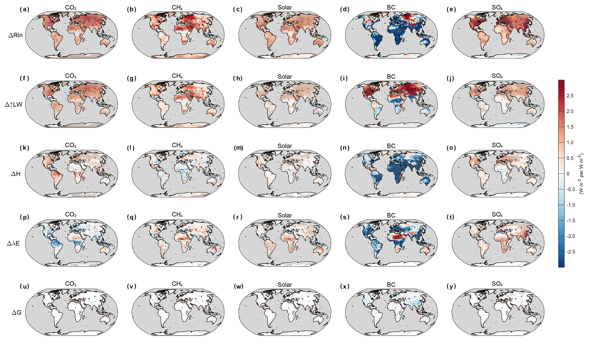
Figure 3MMM changes of R_in and outgoing energy components for all five experiments in the fsst simulations. All changes are normalized to changes per unit of global forcing. Grey dots indicate that the MMM changes are significant at a p value of 0.05.

These changes are obvious when averaged globally (Fig. 4a and Table 2). The R_in decreases by $-\mathrm{3.56}\pm \mathrm{0.60}$ W m⁻², and the H and λE decrease by $-\mathrm{2.88}\pm \mathrm{0.43}$ W m⁻² and $-\mathrm{1.54}\pm \mathrm{0.27}$ W m⁻², respectively, making the energy partitioned to Δ↑LW positive (0.86±0.36 W m⁻²). In other words, although the radiative heating (R_in) decreases, convective and evaporative cooling decrease by a greater amount (124 % relative to ΔR_in) owing to less efficient energy dissipation, thereby warming the surface and leading to a positive Δ↑LW radiation. The reduction of turbulent fluxes (H and λE) is found for both source regions and non-source regions (Fig. 4b). In the source regions, the reductions of turbulent flux are nearly the same as the reduction of R_in, making the temperature response negligible or only slightly negative. In the non-source regions, the reduction of turbulent fluxes exceeds the reduction of R_in, making the temperature response positive. Another interesting phenomenon is that the reduction of H is greater than the reduction of λE for the BC experiment, both on the global scale and in the source regions (Fig. 4). The greater reduction of H indicates a decrease in Bowen ratio (β), defined as the ratio of sensible heat flux over latent heat flux. Globally, β decreases by $-\mathrm{0.20}\pm \mathrm{0.07}$ in the BC case, and such a drop could reach −0.3 in the source regions. In comparison, under other forcing agents, the changes of β are much smaller (the global MMM changes within ±0.10). The larger change of H is somewhat contradicting to the common sense that λE dominates the turbulent flux on a global mean scale. This is because on a global scale, 85 % of λE is from the ocean (Schmitt, 2008). In this study, we only focus on land grids, in which the λE is largely suppressed.

Table 2Globally averaged multi-model mean (MMM ± 1s.e.) values of changes in surface energy components and temperature per unit of global TOA forcing.

Download Print Version | Download XLSX

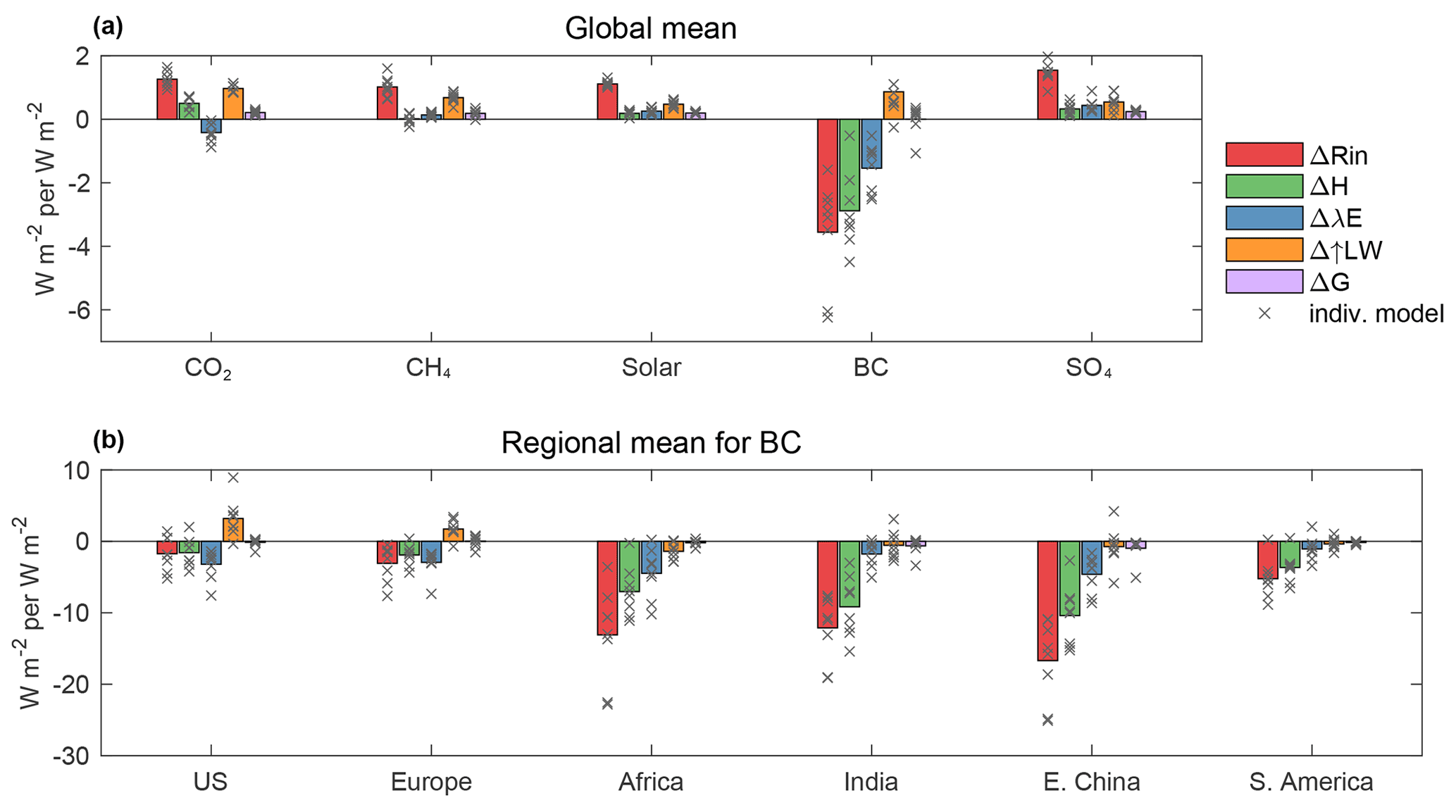
Figure 4Domain-averaged values of R_in and the components of E_out from the fsst simulations for global mean (a) and for selected regions under BC forcing (b). × indicates the values from individual models.

Download

Under other forcing agents, the spatial patterns of Δ↑LW are similar to the patterns of ΔR_in. The changes of H and λE are relatively small and sometimes cancel each other out, making little contributions to temperature change compared with BC (Figs. 3 and 4a). Therefore, the temperature change (Δ↑LW) is dominated by the change of radiative heating (ΔR_in). It is worth noting that the decrease in λE in the CO₂ experiment is due to the physiological effect of vegetation and plantation (Fig. 3p), which is included in the PDRMIP models (Richardson et al., 2018). It is also noted that the stronger responses in the BC scenario (Figs. 3, 4 and Table 2) could be partially related to its larger changes of surface radiative heating (ΔR_in) compared with other forcing agents. Taking CO₂ as an example, ΔR_in is 1.26 W m⁻², similar to its TOA forcing (1 W m⁻²), whereas for BC, ΔR_in is roughly 3 times larger (Table 2). Observations show that the surface forcing of BC could be 10 times larger than TOA forcing on regional scales (Magi et al., 2008), indicating that BC could cause stronger changes of surface forcing than TOA forcing relative to other forcing agents. The contributions of G are negligible (Fig. 3u–y) and will not be further discussed.

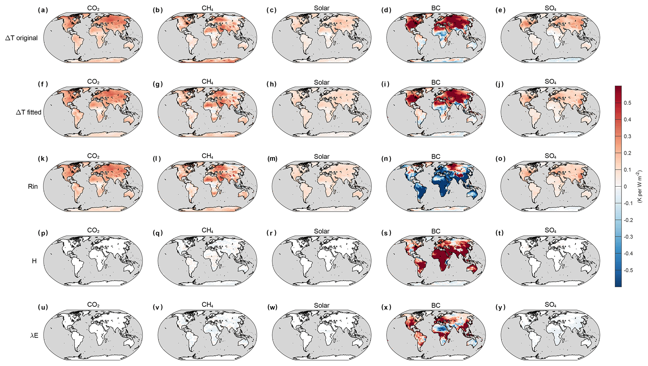
Figure 5Air temperature change per unit of forcing. Original ΔT (a–e), ΔT estimated from multi-linear regression model (f–j), and temperature change contributed by each component based on the linear regression models (k–y).

Table 3Multi-linear regression model for each experiment.

Download Print Version | Download XLSX

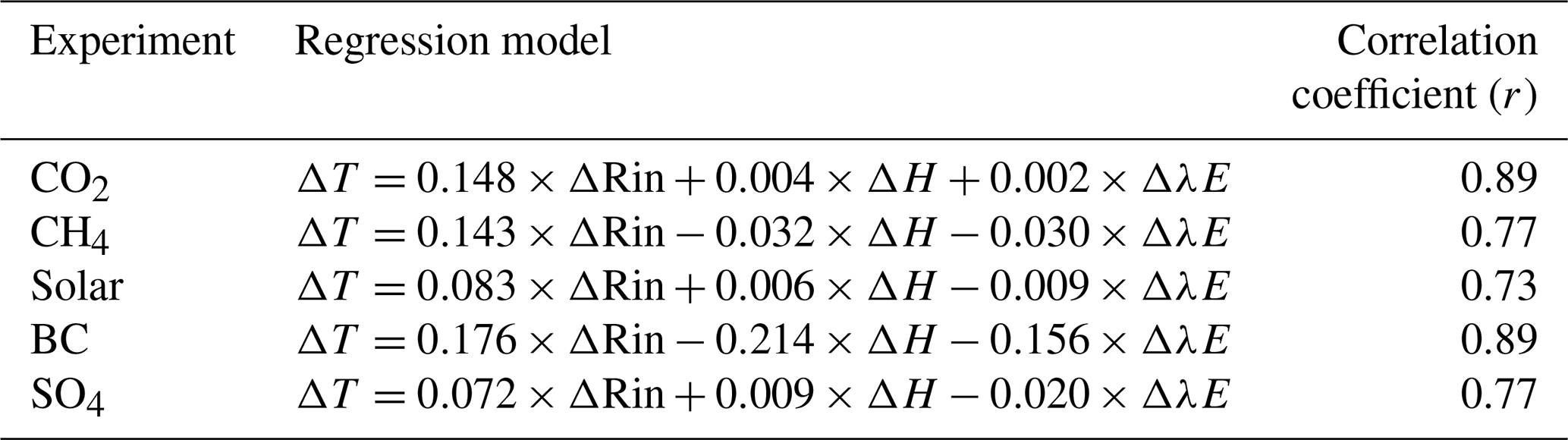
3.3 Attribution of temperature change

In order to quantify the contributions of each component to ΔT, we applied a multi-linear regression model to the MMM values of ΔT and the energy components in each experiment, as $\mathrm{\Delta }T=a\times \mathrm{\Delta }{R}_{\mathrm{in}}+b\times \mathrm{\Delta }H+c\times \mathrm{\Delta }\mathit{\lambda }E$. Here ΔR_in represents the changes of radiative heating, and ΔH and ΔλE denote changes in the surface energy redistribution. All grid cells were given equal weight. The results are listed in Table 3. A point-wise comparison of original ΔT and fitted ΔT is shown in Fig. S1. These regressions reproduce the ΔT fairly well, since the correlation coefficients between ΔT and fitted ΔT are all above 0.73, and most of the data points align along the one-to-one line. For CO₂, CH₄, and solar and sulfate aerosols, the coefficients of ΔR_in are 1 order of magnitude larger than the coefficients of the turbulent fluxes, suggesting that ΔR_in dominates the temperature change under these forcing agents. When it comes to BC, however, ΔT is more sensitive to ΔH, followed by ΔR_in and ΔλE. With the regression coefficients, we estimated the contributions of each energy component to ΔT (Fig. 5). In line with our previous results, ΔT was dominated by surface heating (ΔR_in) for most forcing agents with a very limited role from turbulent fluxes. BC, nonetheless, is an exception. For BC aerosols, ΔT is influenced by both surface heating and turbulent fluxes, with the cooling from the former being overwhelmed by the warming from the latter (Fig. 5n, s, and x). The domain-averaged changes for the BC experiment are listed in Table 4. Globally, ΔH produces 0.19 K warming, and ΔλE leads to 0.07 K warming. The combined 0.26 K warming is offset by −0.19 K cooling attributed to reduced ΔR_in, producing a net warming of 0.07 K. In terms of percentage, ΔH and ΔλE contribute 73 % and 27 %, respectively, to the total warming. Such patterns are also seen on regional scales. The warming contributions from ΔH were 40 % (US), 47 % (Europe), 76 % (E. China), 87 % (India), 68 % (Africa), and 82 % (S. America), and the remaining part was contributed by ΔλE.

3.4 Mechanisms underlying the reduction of turbulent fluxes

The above analyses show that for most of the forcing agents, ΔR_in dominates the surface temperature response, while for BC, the surface energy redistribution also comes into play in modifying temperature response as a result of the significant reductions of turbulent fluxes. The next question is why turbulent fluxes decrease substantially in response to BC particles. According to the bulk parameterization of turbulent fluxes, the sensible heat flux is expressed as $Q_{\mathrm{SH}}=\mathit{\rho }{C}_p{C}_{H}U(T_{\mathrm{s}}-T_{\mathrm{a}}$) and latent heat flux as $Q_{\mathrm{LH}}=\mathit{\rho }{L}_v{C}_{E}U(q_{\mathrm{s}}-q_{\mathrm{a}}$). In these two equations, ρ is air density, C_p and L_v are air specific heat capacity and latent heat of vaporization, respectively; C_H and C_E are two exchange coefficients; U denotes surface wind speed; and (T_s−T_a) and (q_s−q_a) represent temperature gradient and humidity gradient between the surface and air, respectively. In the rapid adjustment stage, wind speed (U) and temperature gradient are the two possible causes for the changes of sensible heat, while wind speed and humidity gradient (q_s−q_a) are likely to drive the change of latent heat flux.

Table 4Domain-averaged T and contributions from each radiative component estimated from the linear regression model for the BC experiment (unit: K).

Download Print Version | Download XLSX

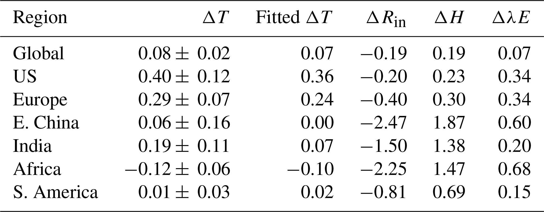
Figure 6a–e show the MMM changes of lower tropospheric stability (LTS), defined as the potential temperature difference between 925 hPa and the surface. An enhanced stability is observed for the BC experiment; ΔLTS is 0.07±0.02 K averaged globally, in contrast to near-zero values from other experiments (−0.01 to 0.01 K). The ΔLTS values for the NH are even larger, with 0.09±0.02 K for BC and −0.01 to 0.01 K for other forcing agents. The enhanced LTS, which can significantly impact the sensible heat flux (Myhre et al., 2018), arises from the fact that the BC layers warm faster relative to the surface due to BC absorption of solar radiation. The changes of LTS patterns are similar for 850 and 700 hPa (Fig.  S2).

Figure 6MMM changes for lower tropospheric stability (LTS, a–e), surface wind velocity (f–j), and humidity gradient (k–o) per unit of global TOA forcing. For LTS, positive anomalies indicate a more stable atmosphere. The humidity gradient is defined as the specific humidity difference between the surface and 850 hPa. Grey dots indicate that the MMM changes are significant at a p value of 0.05.

Figure 6f–j portray the MMM changes of surface wind speed. BC causes a much larger decrease in wind speed with respect to other forcing agents, 0.05±0.01 m s⁻¹ globally compared with zero from other forcing agents. The reduction in wind speed explains the weakening in both sensible and latent heat fluxes according to the bulk parameterization. Figure 6k–o show the changes of humidity gradient (q_s−q_a), defined as the specific humidity difference between the surface and 850 hPa. For CH₄, solar radiation, and SO₄, the gradient increases globally with values of 0.02 g kg⁻¹ (W m⁻²)⁻¹, 0.01 g kg⁻¹ (W m⁻²)⁻¹, and 0.01 g kg⁻¹ (W m⁻²)⁻¹ respectively, causing an increase in λE (Figs. 3 and 4). For CO₂, the gradient shows slightly negative values (−0.002 g kg⁻¹ per W m²), corresponding to reduced λE (Figs. 3 and 4). In terms of BC, the humidity gradient increases by 0.06±0.02 g kg⁻¹ (W m⁻²)⁻¹, but with reduced λE flux, indicating that humidity gradient is not the primary driver of latent heat change. These analyses illustrate that humidity gradient may also influence latent heat flux for CO₂, CH₄, solar radiation, and scattering aerosols. For BC, on the other hand, change of wind speed should be the primary driver of the reduction of λE, and humidity gradient is of less importance.

Now the last question is why the surface wind speed decreases under BC forcing. The first potential explanation is the abovementioned enhanced LTS. Jacobson and Kaufman (2006) has clearly demonstrated that the enhanced LTS and reduced turbulent exchange can reduce the turbulent kinetic energy and vertical transport of horizonal momentum, thereby reducing surface wind speed. The second possible explanation is that from the dynamical perspective, wind speed is controlled by the pressure gradient force (PGF), the Coriolis force, the gravitational force, and the frictional force. PGF is the driving force for atmospheric motion and is potentially the main driver for the changes of wind speed in the current idealized experiments. On a global scale, the excessive heating in the tropics with respect to middle and high latitudes causes PGF to point toward polar regions. Here we hypothesize that the decrease in temperature gradient between the Equator and poles under BC forcing weakened the PGF and slowed down the wind speed. Evidence in support of this hypothesis is found in Fig. 7a–e showing the zonal mean atmospheric temperature change. Mechanistically, BC caused a larger atmospheric heating in the middle latitudes of NH (30–60^∘ N) relative to tropics due to more of the BC forcing being located at middle latitudes of NH (Fig. 7d). The faster warming of middle latitudes weakened the PGF between the Equator and polar regions, as seen from the larger increase in geopotential height of 500 hPa in the middle-latitude regions (Fig. 7i). These patterns are not observed in the other experiments. The changes of geopotential height at other levels show similar results (Fig. S3).

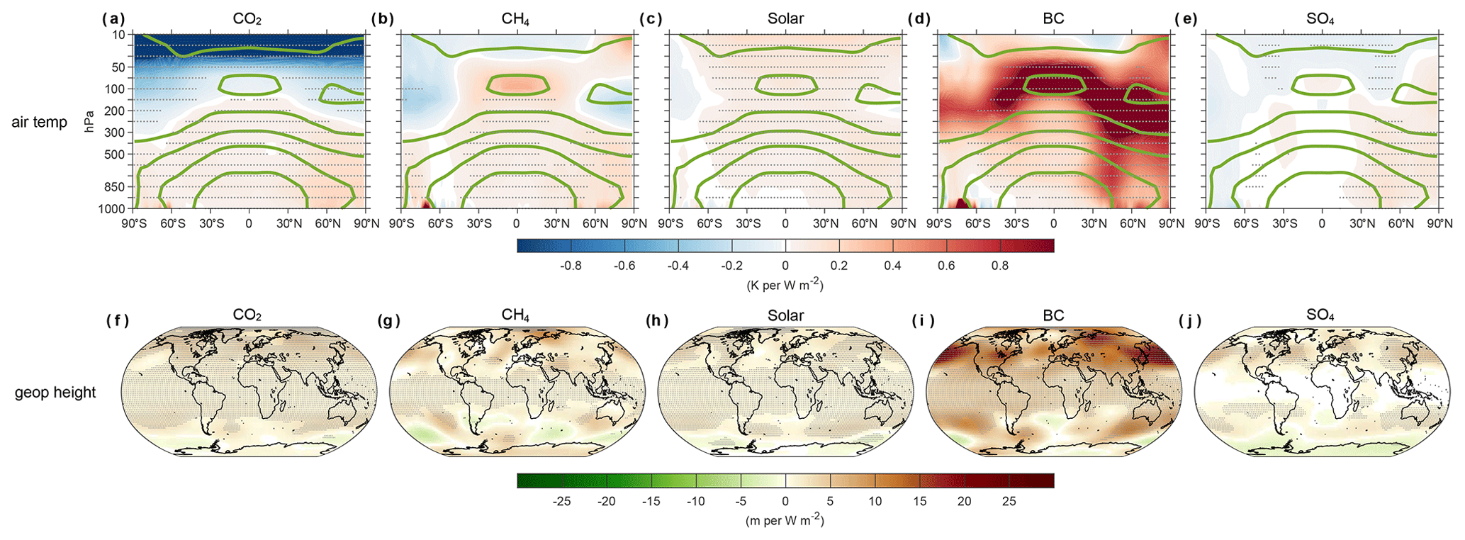
Figure 7MMM changes for zonal atmospheric temperature (a–e) and geopotential height of 500 hPa (f–j) per unit of global TOA forcing. The thick green lines in the upper row are the climatology temperature in the control simulation. Grey dots indicate that the MMM changes are significant at a p value of 0.05.

To further understand the relationship between changes in wind speed and temperature, we defined a temperature gradient index (Allen et al., 2012) as $\mathrm{2}\times \mathrm{\Delta }{T}_{\mathrm{30}-\mathrm{60}}-(\mathrm{\Delta }{T}_{\mathrm{0}-\mathrm{30}}+\mathrm{\Delta }{T}_{\mathrm{60}-\mathrm{90}})$, where ΔT is the mass-weighted (300–850 hPa) temperature response, and subscripts 0–30, 30–60, and 60–90 denote low (0–30^∘ N), middle (30–60^∘ N), and high (60–90^∘ N) latitudinal zones, respectively. When the index becomes more positive, middle latitudes warm faster, and a stronger reduction of wind speed is expected. The results for each individual model and experiment are shown in Fig. 8. A reasonably good correlation is seen in the BC scenario ($r=-\mathrm{0.59}$): a larger change in the temperature gradient index corresponds to a stronger decrease in wind speed. The results for other experiments are mostly scattered around zero.

On regional and local scales, several other factors might also contribute to surface wind change (Wu et al., 2018). For instance, the aerosols in Asia have been reported to modify the land–sea temperature contrast and thus modify monsoon circulation (Xu et al., 2006; Meehl et al., 2008). The different phases of internal variability (e.g., El Niño–Southern Oscillation (ENSO) and North Atlantic Oscillation (NAO)) could modulate the circulations on interannual to multi-decadal timescales (Jerez et al., 2013; Hu and Fedorov, 2018). Bichet et al. (2012) suggested that changes in the surface roughness length may also change the wind speed. These factors are not considered in the present study.

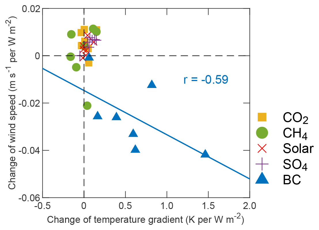
Figure 8Changes of wind speed versus changes of temperature gradient for each individual model and simulation. The CESM1-CAM4 model is excluded due to the unavailability of surface wind data. The linear correlation r is for the BC experiment.

Download