Detailed Patterns of Methane Distribution in the German Bight

Introduction

The levels of atmospheric methane (CH₄) have increased rapidly worldwide since 2005 (IPCC et al., 2013). However, the exact reasons for this increase are not completely clear. The average estimated contribution of world oceans to the global CH₄ budget is 13 Tg CH₄ y^–1, which accounts for 3.5% of the yearly emissions from natural sources. However, the range of estimates is large, from 9 to 122 Tg CH₄ y^–1 (Saunois et al., 2016, 2020). This global oceanic flux of CH₄ is dominated by shallow near-shore environments, where CH₄ released from the seafloor can escape to the atmosphere before oxidation. However, the uncertainty of CH₄ flux estimations in coastal areas is especially large, with values ranging from 0.8 to 3.8 and an average of 2.1 ± 1.6 Tg CH₄ y^–1 (Weber et al., 2019). This hinders the reliable estimation of the contribution of oceans to global CH₄ budget calculations. Therefore, there is a need to improve observational capacities focusing on shallow coastal marine environments by using high temporal and spatial sampling resolutions to capture sharp coastal gradients of CH₄ concentrations (Weber et al., 2019), which would provide a better baseline for estimating the role of coastal zones in the global methane budget.

The CH₄ budget of the central North Sea is characterized by pockmarks (Krämer et al., 2017), drilling activities (Vielstädte et al., 2017), and gas ebullition sites (Mau et al., 2015; Römer et al., 2017). In contrast, in the southern North Sea and areas close to the mainland, dissolved CH₄ mainly originates from autochthonous methanogenesis in sediments (Yin et al., 2019) with subsequent flux into the water column, tidal flats (Røy et al., 2008; Wu et al., 2015), or riverine input (Upstill-Goddard and Barnes, 2016). Borges et al. (2017) showed that warm summers in northern Europe in recent years have increased CH₄ concentrations to enhanced methanogenesis, which has led to higher CH₄ fluxes at the Belgian coast (Borges et al., 2017, 2019). In addition to climatic changes, the southern North Sea is also heavily affected by anthropogenic impacts related to agricultural land use and wastewater discharge. These factors significantly change the source, rate, and pathways of CH₄ production, thereby leading to a net increase in emissions from estuaries (Wells et al., 2020). Previous studies have investigated the temporal and spatial patterns of CH₄ between Helgoland, the coast (Cuxhaven), and the Elbe River (Hamburg) on a monthly basis from 2010 to 2014 (Osudar et al., 2015; Matousu et al., 2017). In these studies, the CH₄ concentrations near the coast ranged between 30 and 40 nmol L^–1, whereas near Helgoland, the concentrations were 14 ± 6 nmol L^–1.

The influence of factors determining the methane concentration in coastal waters is complex and difficult to identify. Previous studies have shown that only approximately 57% of the overall methane variability can be explained, mostly by salinity (Osudar et al., 2015), whereas the influence of turbidity on aquatic CH₄ concentration is still a matter of debate. Osudar et al. (2015) did not observe any relevant correlation between CH₄ concentration and suspended particulate matter (SPM) in the North Sea. However, other studies in tropical estuaries and tidal marshes reported higher methane concentrations upon increased turbidity induced by high tide or sediment resuspension (Trifunovic et al., 2020; Li et al., 2021). Complex relationships between methane and turbidity have also been reported in other areas (Upstill-Goddard and Barnes, 2016).

Previous studies (Osudar et al., 2015; Matousu et al., 2017; Hackbusch et al., 2019) have provided highly necessary data on methane concentrations in the southern German Bight for a range of several years. However, their spatial resolution is rather low, with discrete sampling stations located 10–20 km apart. Therefore, we used methane measurements at higher spatial resolution to obtain more insight into the complex relationship between methane and its influencing factors in the southern German Bight.

Study Area

The relatively shallow (10–43 m) German Bight is situated in the southeastern part of the North Sea, and its topography is dominated by the ancient Elbe River valley (Figure 1). The Wadden Sea is a shallow coastal sea (<10 m) that borders the German Bight along the Dutch, German, and Danish coasts (van Beusekom et al., 1999). The distributions of temperature and salinity in the bottom layers of the German Bight are strongly correlated with topography and follow the ancient Elbe River valley (Becker et al., 1999). The German Bight is dominated by a mostly counterclockwise residual circulation pattern, which carries a mixture of Atlantic water and continental runoff from the Rhine and several other rivers into the German Bight from the west. The central part of the North Sea is seasonally stratified, whereas the southeastern German Bight and Wadden Sea regions are generally well mixed because of strong tidal currents (Becker et al., 1999).

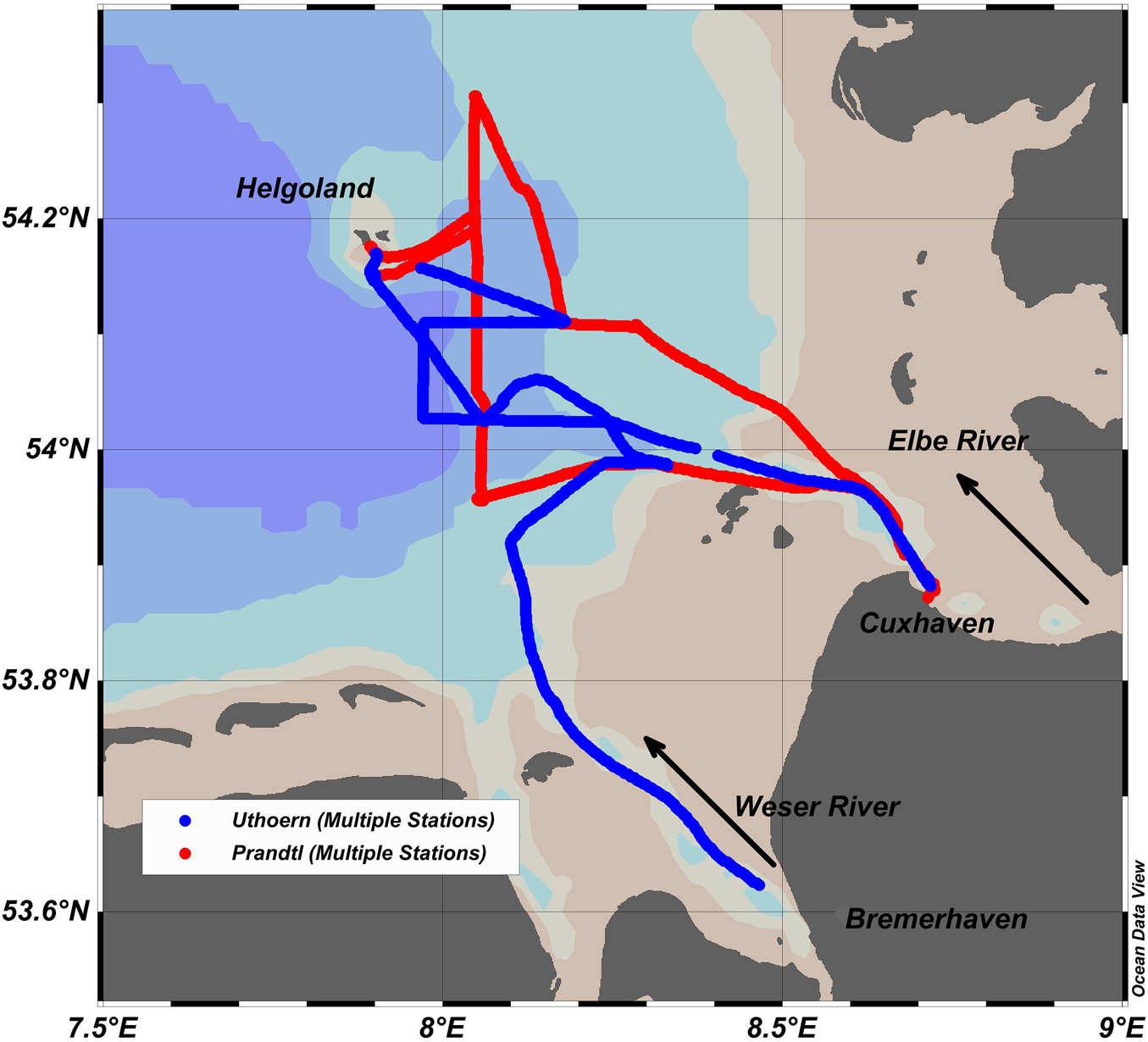
Figure 1. Cruise track of RVs Uthörn in blue and Ludwig Prandtl in red on 25 and 26 June 2019.

The water in the German Bight is not static. It moves with tidal currents (mostly back and forth in quasi-ellipsoids) and presents a prevalent overall pattern (residual circulation) with water usually moving counterclockwise entering the German Bight from the east and leaving toward the north (Nauw et al., 2015). These temporal and spatial dynamics of the water masses should be considered when backtracking the source of methane observed in different parts of the target area with partly small-scale elevated concentrations.

The Elbe is one of the largest rivers in northern Europe, with an approximate length of 1,100 km. It is the main source of freshwater to the inner German Bight, with a median discharge of 409 m³ s^––1 (2000–2019¹). The Weser River estuary is associated with a median discharge of 212 m³ s^––1 (2000–2019²). The outer estuary is characterized by a funnel-like morphology with extensive open tidal flats. The mean tidal range exceeds 3.5 m, but water levels are also influenced by strong winds. Because of the high current velocities in the estuary, the water is generally well mixed and highly turbid, with a weakly stratified salt wedge (Schuchardt et al., 1993).

Materials and Methods

Study Sites

The cruise Stern 2 was held on June 25 and 26, 2019, as part of the project Modular Observation Solutions for Earth Systems (MOSES), event chain Hydrological Extremes³. On June 25, two ships departed from Cuxhaven following the main shipping route (Figure 1). Research Vessel (RV) Uthörn (Figure 1, blue) followed a northwesterly course, whereas RV Ludwig Prandtl (Figure 1, red) followed a more westerly route, passing the island of Scharhörn. At approximately 8°E, RV Ludwig Prandtl turned straight north, crossed the Uthörn track, headed further north until the Helgoland latitude, and then turned toward the port of Helgoland. RV Uthörn sailed more toward the west and followed a zigzag line, finally heading toward Helgoland. The next day (June 26), RV Ludwig Prandtl headed to the northernmost station at 54.3°N. It then finished the west-east track at 8.3°E and returned to Cuxhaven. RV Uthörn returned to the meeting point of June 25, followed by a crisscrossing of the expected Weser water plume, and finally entered the Weser toward the Bremerhaven Port (Figure 1). More details can be found in the cruise report (Bussmann et al., 2020).

Additional data used in the present analysis were obtained from three cruises between Helgoland and Cuxhaven in the autumn and winter (October 10, November 7, and December 6) of 2018 (Winkler, 2019⁴).

Water Supply for Underway Systems

Methane and hydrographic parameters were continuously measured using a basin that was continuously flushed with surface water. On RV Uthörn, a water basin with a volume of 65 L was continuously refilled with sea water at a flow rate of approximately 60 L min^–1. The inlet of the water supply was located in the bow of the ship at a water depth of approximately 1 m. On RV Ludwig Prandtl, a similar water basin was used with a volume of 10 L and flow rate of approximately 2 L min^–1. Previous studies have shown that the analysis with the described system (GGA and ship’s water supply) or classical water samples taken from a rosette with Niskin bottles did not change the CH₄ concentrations (Winkler, 2019).

Hydrographic Parameters

In the RV Ludwig Prandtl, the built-in FerryBox (Petersen, 2014) recorded data using a Teledyne RDI thermosalinograph (temperature and salinity), Aanderaa oxygen optode 4330 (oxygen concentration and saturation), Meinsberg pH electrode (pH values), and SCUFA submersible chlorophyll fluorometer (turbidity and fluorescence). The data were stored on board and automatically sent via a mobile phone connection to the Hereon database. The water flow in the FerryBox was approximately 12 L min^–1. On the RV Uthörn, a portable pocket FerryBox (4H-Jena, Germany) was used to record the hydrographic parameters using the following sensors: Seabird SBE45 thermosalinograph, Aanderaa oxygen optode, Meinsberg pH electrode, Seapoint Chlorophyll Fluorometer (SCF), and Seapoint Turbidity Meter. The water flow was between 3 and 4 L min^–1. Data were saved once per minute.

Methane Analysis

Methane was measured both by discrete samples of surface water using Niskin bottles attached to a rosette and by a continuous underway sampling system for methane fed from the basins. The dissolved CH₄ concentrations in the continuous water supply were measured with a dissolved gas extraction unit and a laser-based analytical Greenhouse Gas Analyzer (GGA; both Los Gatos Research, United States) on both ships. On the RV Uthörn, the GGA was a micro portable GGA, whereas the RV Ludwig Prandtl used a bigger lab version. The degassing units withdrew water from the water basins at 1.2 L min^–1. CH₄ was extracted from the water via a hydrophobic membrane and hydrocarbon-free carrier gas on the other side of the membrane (synthetic air or nitrogen, at 0.5 L min^–1). The carrier gas and extracted CH₄ were then directed to the inlet of the gas analyzer. The time offset between the water intake and stable recording at the GGA was determined beforehand in the laboratory. The total offset (water supply + instrument offset) was 394 and 219 s for the setup on the RV Ludwig Prandtl and RV Uthörn, respectively.

To convert the relative concentrations (ppm) given by the GGA to absolute concentrations (nmol L^–1), discrete water samples were obtained at least every hour. The CH₄ concentration in these bottles was determined using the headspace method and gas chromatographic analysis (see supplement). Based on the obtained values, the conversion factors (ppm to nmol L^–1) of 19.33 and 39.51 were determined for the setup of RV Ludwig Prandtl and RV Uthörn, respectively.

Carbon Isotopic Signal of CH₄

The bottles used for the headspace analysis of CH₄ concentration were also used to determine the δ¹³C of CH₄ using a Delta XP plus Finnigan mass spectrometer. The gas (20 mL) was removed with a glass syringe, replaced by adding 20 mL of a saturated NaCl solution, and injected into the septum of a fixed gas sampling device. The extracted gas was purged and trapped with a PreCon equipment (Finnigan, Thermo Fisher Scientific, United States) to pre-concentrate the sample. The carbon isotopic ratios were relative to the Vienna Pee Dee Belemnite (VPDB) standard according to conventional annotation. The analytical error of the ¹³CH₄ values were ± 1.6‰. Ambient compressed air (set to −47.4‰) and an isotope gas standard (−54.5 ± 0.2‰, B-iso1, Isometric Instruments, Canada) were used for calibration. The median difference between duplicate water samples was ± 0.6‰.

Calculation of Diffusive CH₄ Flux

The overall gas exchange across an air–water interface can be described by Wanninkhof et al. (2009):

where F is the rate of gas flux per unit area (μmol m^–2 d^–1), c_m is the measured CH₄ concentration of the surface water, and c_equ is the atmospheric gas equilibrium concentration (Wiesenburg and Guinasso, 1979). Atmospheric CH₄ concentration data were obtained from the meteorological station in Mace Head, Ireland, via the National Oceanic and Atmospheric Administration, Earth System Research Laboratory, Global Monitoring Division⁵ as the monthly mean of June 2019 (1.928 ppm). The gas exchange coefficient (k) is a function of water surface agitation. The k value in oceans and estuaries is determined mostly by wind speed (U₁₀), whereas water velocity dominates in rivers (Alin et al., 2011). The determination of k is crucial to calculate the sea–air flux. We calculated k₆₀₀ according to the following equation for coastal seas (Nightingale et al., 2000):

The calculated k₆₀₀ (for CO₂ at 20°C) was converted to k_CH4 (Striegl et al., 2012), and the Schmidt number (Sc) was adjusted based on water temperature and salinity (Wanninkhof, 2014):

Wind direction and velocity were measured on board the RV Ludwig Prandtl using a Compact Weather Station (Manual Gill GMX600 sensor) every minute. These wind data were used for the datasets of both ships. When the RV Uthörn entered the Weser estuary, hourly wind data from Bremerhaven (8.158E, 53, 785N, German Meteorological Service⁶) were used.

We compared our recent data with previous datasets, including data obtained from stations sampled in the same month (June) from 2010 to 2014 (Bussmann et al., 2014, 2019). To calculate the diffusive flux from this dataset, average daily wind data were obtained from the German Meteorological Service for the stations of Helgoland and Cuxhaven.

Data Management and Handling

All data used in the manuscript are available in the AWI-sensor net data repository⁷. Metadata information were obtained from the expedition report (Bussmann et al., 2020). All data were referenced by time (UTC), allowing for an easy combination. The data were freely available for downloading.

To ensure comparability of the relevant parameters (temperature, salinity, and CH₄) measured with different sensors on the two ships, two intercalibration intervals were defined during the cruise. At the beginning of each day (June 25 and 26), the ships stayed near each other (60–500 m) for 30 min, with all underway systems running. At the end of this time, a vertical profile was measured on both ships, discrete water samples were collected, and a CTD profile (conductivity, temperature and density sensor) with temperature and salinity was determined.

To ensure inter-ship comparability of temperature measurements, we first compared the deep profiles (50 m) of the two in situ CTDs on both ships. The measurements were in good agreement (r² = 0.98, slope and intercept were not significantly different from 1 and 0, respectively). Therefore, we assumed they reflected well the real in situ temperature. To ensure comparability of temperature measurements within each ship, we compared temperatures obtained from surface water (0.5–2 m water depth) of the respective CTDs and those obtained by the ship underway systems (FerryBox), and we calculated the offset between them. The average offsets of the FerryBox temperature measurements to the CTD measurements for RV Ludwig Prandtl and RV Uthörn were −0.76 ± 0.10°C (n = 22) and −0.34 ± 0.14°C (n = 35), respectively, and data were corrected accordingly.

To ensure inter-ship comparability of salinity measurements, water samples were collected from both ships at several stations and depths. All water samples were analyzed for salinity using an Optimare Precision Salinometer System. As we focused on surface water, only the FerryBox data on salinity were used for comparison with the salinity of water samples. There was a wide range of salinity measurements compared to the relatively homogenous water temperature. Therefore, linear regression was applied to compare the salinity measurements of the underway system with the discrete samples. The linear regression revealed no significant differences in the slope to 1 and no significant difference in the intercept to 0 for both ships. Therefore, the salinity data from the underway systems were used without further modification.

For CH₄, the intercalibration data could not be used because the values were not stable over time, which was likely caused by the exceedingly short runtime after starting the devices. Therefore, we considered a time on June 25 when both ships were cruising in parallel heading north of Cuxhaven, with a median difference of 0.004° latitude and −0.006° longitude. Comparing these data, we calculated the median difference in CH₄ concentrations of 7.8 nmol/L. At four other locations, the ships crossed the same position. However, that occurred with a 6–90 min delay, for which a difference of 7.1 nmol/L was calculated. Considering all these factors, we added 7.7 nmol/L to all CH₄ concentrations measured on the RV Ludwig Prandtl as an intercalibration factor to the RV Uthörn for June 25. For June 26, during the intercalibration time off Helgoland, a median difference of −3.6 nmol/L (n = 12) was measured on the RV Ludwig Prandtl compared to the RV Uthörn, and this value was used to correct all RV Ludwig Prandtl CH₄ data measured on that day.

For calculating the relative importance of the three predictors salinity, temperature and oxygen saturation on the outcome variable (dissolved methane), a multiple linear regression with subsequent bootstrap based LMP metric calculation of the R² contribution was done according to Lindeman et al. (1980) and Chevan and Sutherland (1991). Calculations were done with RStudio, package “relaimpo”.

Additional data on water discharge in 2019 from Elbe and Weser were used in this study. They were obtained from the Wasserstraßen- und Schifffahrtsverwaltung des Bundes (WSV), provided by the Bundesanstalt für Gewässerkunde (BfG) for the Elbe and for the Weser by Flussgebietsgemeinschaft Weser⁸, by Ms I. Krippenstapel.

Backtracking of Water Masses

We applied backward trajectories to acquire insight into the background of the water bodies that were probed. This analysis was performed to help distinguish between temporal and spatial variability, that is, between local changes and advection. Data were retrieved from the Hereon drift app (⁹ last access 26 May 2021). The calculations in this application are based on simulations using the Lagrangian offline transport program PELETS-2D (Callies, 2021) and 2D marine currents extracted from the archived output of the 3D hydrodynamic Federal Maritime and Hydrographic Agency [Bundesamt für Seeschifffahrt und Hydrographie (BSH)] model, BSHcmod (¹⁰ last access 26 May 2021). The data input into the model was marine currents with 0.6% wind drag and travel time of 3 day in the top layer.

Results

Water Mass Characterization

In this study, the two rivers entering the German Bight, namely the Weser and Elbe rivers, were characterized by different water temperatures. At salinity <25, the Weser and Elbe water samples showed median temperatures of 20.9 and 19.3°C, with n = 22 and 275, respectively. At salinity of 25, the Weser and Elbe water samples presented densities of 17.3 and 16.9 kg m^–3, respectively. The water masses leaving the river mouths were mixed with marine water. Approximately at 53.9°N and 8.3°E, the mixed water presented temperature of 18.1°C, salinity of 31.8, and density of 22.8 kg m^–3. The area west of 8°E was the most saline (marine) water, with salinity of 33, temperature of 16.7°C, and density of 24 kg m^–3 (Supplementary Figure S1).

Overall Methane Distribution

As shown in the overview in Figure 2, CH₄ concentrations were higher in the river estuaries and lower in the marine area. For the marine endmember, we observed a robust median CH₄ concentration of 4.7 nmol/L (n = 97, ranging from 4.2 to 17.3 nmol/L) at salinity ≥33. In contrast, the riverine input was more variable. The Weser estuary was investigated only on June 26, whereas the Elbe Estuary was investigated on June 25 and 26. The dilution plots (CH₄ versus salinity) revealed that the dilution of river water into marine water started at a salinity of approximately 25. At salinity <25, the plot of CH₄ versus salinity was a horizontal line with a median slope of zero, and at salinity >25, the slope became negative. More details on the determination of the inflection point can be found in the Supplementary Material. This point of inflection for the Weser was observed for a salinity of 25.6, and for the Elbe, it was observed at a salinity of 24.8 on June 25, and of 25.5 on June 26 (Figures 3A,B; Supplementary Figure S2). For the Weser water, we calculated an average CH₄ concentration of 43.1 nmol/L (n = 17, 44.2 ± 2.3 nmol/L, at S = 17–25, Figure 3A), with maximum values of up to 49 nmol/L at salinity <22 (Figure 3A, upper left box).

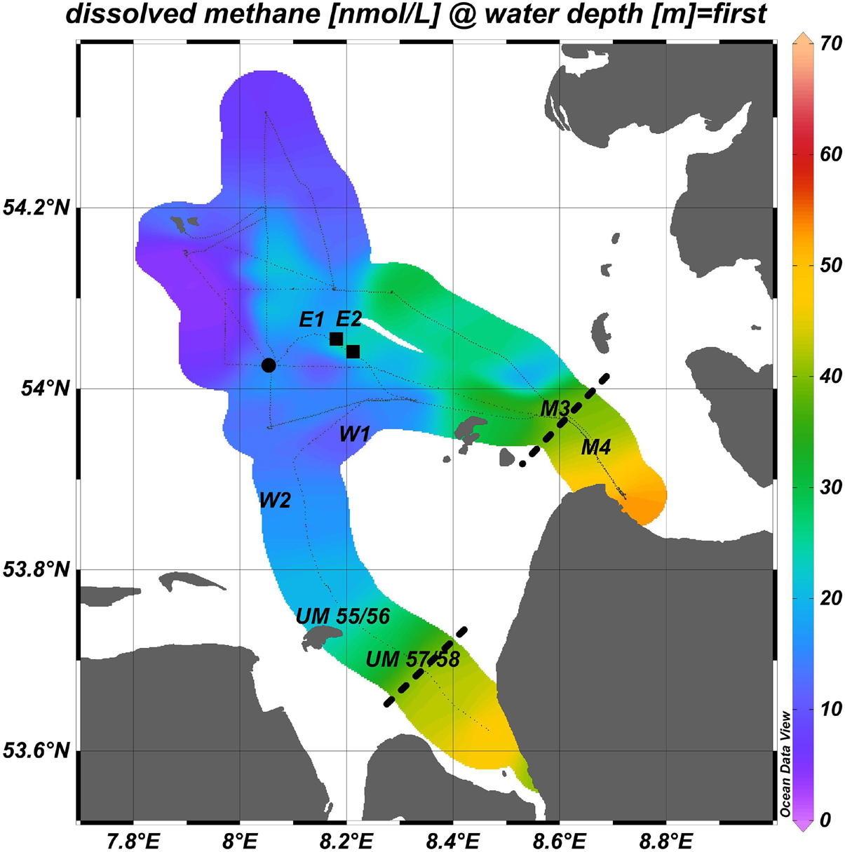
Figure 2. Methane concentrations in surface waters (all data, both days, both ships). The dotted lines indicate the 25-salinity limit. Shown are also the stations where samples for isotopic analyses had been taken (M3, M4, UM55/56, UM57/58). The symbols depict the area of local methane increases, due to increase of oxygen decrease (dot) and turbidity (squares). Indicated are also the stations E1, E2 and W1, W2.

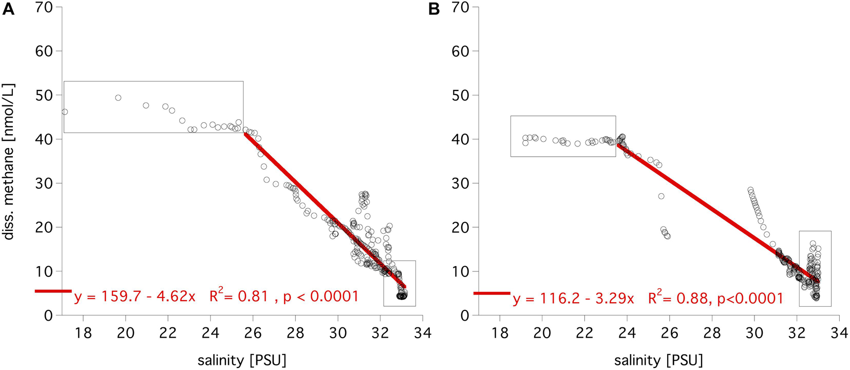
Figure 3. Dilution of river water with marine water on 26 June (A) with Weser water and (B) with Elbe water. The boxes indicate the riverine and marine part. The red line indicates the regression line and its equation.

In the Elbe River, on June 26, the median CH₄ concentration was 39.7 nmol/L (n = 25, 39.6 ± 0.4 nmol/L, at S = 19–23, upper left box in Figure 3B), which is slightly lower than the respective Weser value. The concentrations within the Elbe were relatively stable. However, parts of the marine section clearly did not follow the dilution line. In the Elbe River, on June 26, the median CH₄ concentration was 50.0 nmol/L (n = 194, 50.7 ± 5.4, at S = 19–23 (Supplementary Figure S2), about 10 nmol/L more than on the previous day. However, the CH₄ data in the estuary display a strong variability.

Isotopic Signal

On June 26, when RV Prandtl returned to the Elbe Estuary and RV Uthörn to the Weser Estuary, samples for stable isotope analysis of CH₄ were obtained. The vertical profiles revealed no differences between the surface and bottom samples within each river system, thus data were pooled. Regarding geographic location, M 3/4 samples were obtained in the Elbe outflow, whereas UM 55–58 samples were obtained in the Weser outflow (Figure 2). The isotopic signal for CH₄ in Weser water was slightly heavier (median −52.7‰, n = 3) than that in Elbe water (−56.4‰, n = 2). To determine the extent and location at which it was possible to discriminate the water masses of the rivers Elbe and Weser based on isotopic signatures, we used a Keeling plot to map the delta 13-C signal versus the inverse of the CH₄ concentration. The signal of marine water had a median composition of −48.2‰. The separate plots of the samples from Weser and Elbe revealed no significant differences between the source signals, as the y-axis was intercepted at −56.9‰ ± 0.9‰ and −57.1‰ ± 0.7‰, respectively. Moreover, the overall Keeling plot also revealed no differences (Supplementary Figure S3). Therefore, the signals of the two rivers could not be separated based on isotopic signals.

Influence of Water Mass Origin on the Methane Distribution in Surface Water

In principle, river water is increasingly diluted into seawater with increasing distance from the river mouth. A multiple linear regression analysis revealed that salinity, temperature and oxygen saturation significantly influenced the methane concentration (adjusted r² = 0.89, p < 0.0001). Salinity, temperature and oxygen contributed with 50, 29, and 21% to the overall r² (details see Supplementary Table S1). However, the above results (Figures 3A,B) indicate that the methane concentration pattern in the target area cannot be fully explained by an ideal dilution process. A detailed inspection revealed remarkable spatial patterns, independent from the dilution process. In the following section, we focus on medium- and smaller-scale CH₄ distribution in the target area and the parameters that potentially influence it.

The origin analysis of water masses was applied to target areas that present the same salinity but different CH₄ contents. On June 26, a location at 7.898°E and 54.153°N south of Helgoland (marked as “51” in Figure 4A) and another between Helgoland and Cuxhaven (8.062°E and 54.025°N, blue dot in Figure 4A) were analyzed. Both locations presented the same salinity of S = 32.1, but significantly different CH₄ concentrations of 5 and 10 nmol/L, respectively. By tracing the water masses using the model described earlier, we observed that water from the first station circled around Helgoland for the previous 3 days and, therefore, should have a CH₄ concentration close to the marine background level. In contrast, the water from the second station originated more toward the coast, thus being more affected by tidal flats and river input, which explained the higher CH₄ concentration.

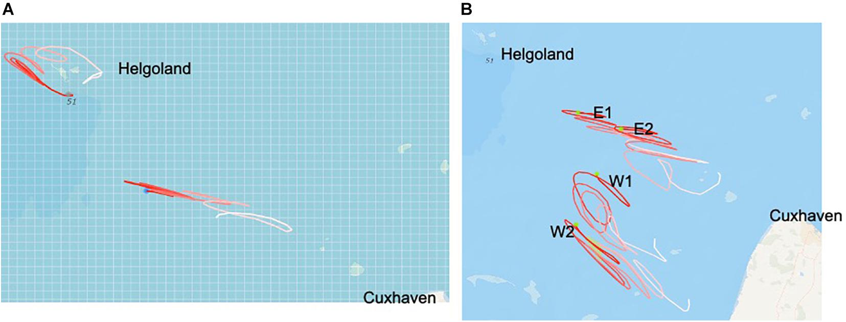
Figure 4. Three day back-trajectories of water mass for (A) two stations near Helgoland and (B) two stations north-west (E1, E2) and west (W1, W2) of Cuxhaven. Green dots indicate the starting position and starting time of the water mass. Red color depicts the starting time, white color depicts the position 3 days before. For a better orientation the island of Helgoland is indicated and the port of Cuxhaven.

Another example of the influence of the origin of water mass on the methane concentration is shown in Figure 4B and further analyzed in Supplementary Figure S4. Supplementary Figure S4 shows the dilution line for the Weser River water (r² = 0.75, p < 0.001) on June 26. At stations E1 and W1, salinity values were both 31.4, but methane concentrations were 20 and 10 nmol/L, respectively. Similar results were observed in stations E2 and W2, where the salinities were 30.1, but E2 presented nearly twice the methane concentration of W2 (27 and 16 nmol/L). The backtracking model revealed that the water mass sampled at stations E1 and E2 originated near the island of Scharhörn and Cuxhaven, and thus likely stemmed from the Elbe River. In contrast, for stations W1 and W2, the backtracking model shows a clear origin within the Weser River.

Influence of Oxygen on the Methane Distribution in Surface Water

Another small-scale patch of elevated CH₄ concentration in the surface water with a spatial extension of 5 km was observed on June 25. When steaming in a westerly direction, CH₄ concentrations decreased continuously, as expected. However, at 8.06°E, 54.02°N, CH₄ concentrations suddenly increased from 9 to 18 nmol/L, followed by a drop to 5 nmol/L (Figures 5A,B). Neither the origin of water masses nor other hydrographic parameters could explain these changes in CH₄ concentrations. However, a hydrographic difference was detected in the oxygen saturation, which showed a distinct decrease to 87% saturation at the exact location of the maximum CH₄ concentration. The correlation between oxygen saturation and CH₄ concentration was significant, with r² = 0.79, and p < 0.001 (Figure 5D). Nevertheless, this local patch of higher CH₄ concentrations was not stable over time. In the next day, elevated CH₄ concentrations were no longer observed.

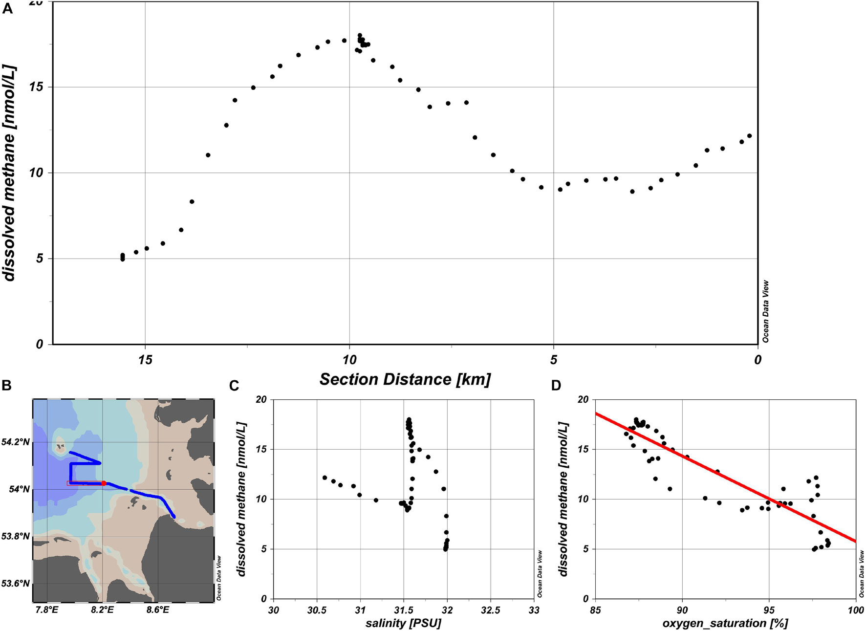
Figure 5. A small-scale increase of methane (A) with the corresponding oxygen saturation (D). The section is shown in (B), and the section distance is recorded from east to west, starting with the red dot. Shown is also the correlation to salinity (C).

Influence of Turbidity on the Methane Distribution in the Surface Water

As the turbidity dataset was not complete, a detailed analysis of the relationship between turbidity and methane concentration was not possible. Therefore, we used turbidity data from the autumn and winter 2018, for similar transects sampled between Helgoland and Cuxhaven (Winkler, 2019). During this time, identical assessments were performed using the exact same instrumental setup for methane and a CTD for hydrographic parameters. Elevated CH₄ concentrations of 60 and 20 nmol/L were observed in two cruises in November and December, respectively, at almost the same location (8.2°E, 54.05°N), and background CH₄ values of approximately 10 nmol/L were measured (Figure 6A). In contrast, no such elevated CH₄ concentrations were observed in October. Neither salinity nor water mass origin or bottom features could explain the elevated CH₄ concentrations. During these cruises, a significant correlation between turbidity and CH₄ concentration was observed (November: r² = 0.74, p < 0.001; December: r² = 0.62, p < 0.001; Figure 6D).

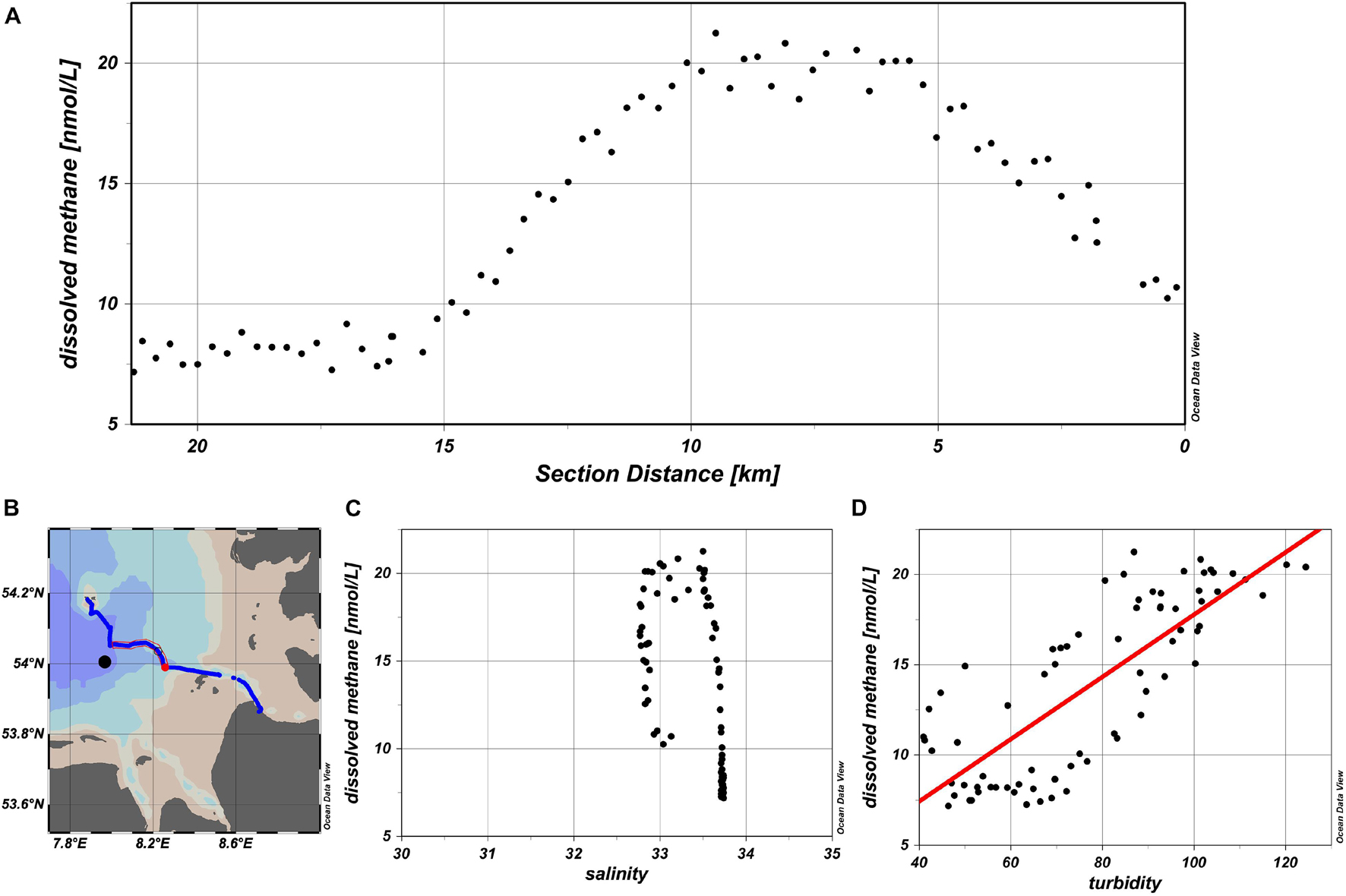
Figure 6. A small-scale increase of methane (A) with the corresponding turbidity (D) in December 2018. The section is shown in (B), and the section distance is recorded from east to west, starting with the red dot. Shown is also the correlation to salinity (C).

Diffusive Methane Flux

The diffusive flux of CH₄ from water into the atmosphere provides an estimate of the input of CH₄ from coastal waters to the atmosphere. On June 25, the weather was calm with a median wind speed of 5.5 m s^–1, ranging from 3.3 to 9.6 m s^–1, which resulted in a gas exchange coefficient (k) for CH₄ of 0.9–10.6 m d^–1, with a median value of 2.4 m d^–1. On June 26, wind conditions were rougher, with a median wind speed of 9.0 m s^–1, and values ranging from 6.4 to 13.4 m s^–1. On June 26, k ranged from 3.2 to 12.7 md^–1, with a median of 6.1 m d^–1.

To provide a realistic CH₄ flux estimate for the target area, we divided the area into five sub-areas based on their salinity (Supplementary Figure S5). In the northeastern part of the target area, the area with salinity >30 was defined as a fully marine area. The diffusive methane flux in the marine area was 40 ± 29 μmol m^–2 d^–1 (n = 591 Supplementary Table S2). Toward the coast, the two mixing areas (northern and southern) were characterized by salinity of 29.9 > S > 25.1, with methane fluxes of 86 ± 34 μmol m^–2 d^–1 (n = 118) and 122 ± 40 μmol m^–2 d^–1 (n = 53, Supplementary Table S2), respectively. The river estuaries were defined by salinities <25, with a methane flux of 124 ± 42 μmol m^–2 d^–1 (n = 297) for the Elbe Estuary and 214 ± 61 μmol m^–2 d^–1 (n = 25) for the Weser estuary (Supplementary Table S2).

Discussion

Comparison With Previous Data

Previous data on CH₄ concentrations between the Elbe mouth at Cuxhaven and the Helgoland area were available from 2010 to 2014, based on monthly cruises with fixed stations and discrete water samples (Osudar et al., 2015; Matousu et al., 2017; Hackbusch et al., 2019). In June of 2019 and 2010–2014, similar average CH₄ values in the Elbe (S < 24.9) were observed, at 49 and 51 nmol/L, respectively. Data on the CH₄ content of Weser were even more sparse. Grunwald et al. (2009) reported rather high concentrations of 300–1,600 nmol/L in 2003, but own measurements in November 2019 (Bussmann et al., 2021) and in this study revealed significantly lower concentrations in the Weser near Bremerhaven, at 56 nmol/L (Bussmann et al., 2021) and 43 nmol/L, respectively. In the coastal area (25 < S < 29.9), CH₄ presented a slight decrease from 2010 to 2014, with an average of value 39 nmol/L, in contrast to the 28 nmol/L identified in 2019. In the marine area around Helgoland, the CH₄ content in 2010–2014 was distinctively higher than that in 2019, with average values of 23 and 12 nmol/L, respectively. The higher CH₄ concentrations around Helgoland in the previous years may partly be explained by the overall lower salinities >30 in 2010–2014, compared to >33 in 2019.

In the central North Sea, methane concentrations lower than 50 nmol/L have been reported for surface waters (Mau et al., 2015). At the Belgian North Sea coast, significantly higher values have been reported, with an average of 48–61 nmol L^–1 in May 2016 and 2018 for all stations up to 50 km offshore (Borges et al., 2019). Compared to these data, our overall average of 22.9 ± 14.9 nmol L^–1 is significantly low.

The dilution of CH₄-rich water in CH₄-poor marine water started at salinities of approximately 25 in the Elbe and Weser estuaries. A similar pattern was observed from the Schelde River (Borges and Abril, 2012; Jacques et al., 2020). In several British estuaries, a decrease in the CH₄ content was observed for salinities above ∼20, similar to the results observed in our study (Upstill-Goddard and Barnes, 2016). Upstill-Goddard and Barnes (2016) showed that higher concentrations in the upper estuary may be the result of a lateral input of tidal marshes. This is probably the case for the Elbe and Weser estuaries, as higher concentrations and high variability at S < 25 were observed in the Weser (Figure 3A) and Elbe estuaries (Supplementary Figure S2), respectively, which suggests an input from other CH₄ sources, such as tidal flats or small rivers. Therefore, this should be considered when interpolating CH₄ concentrations of a river endmember based on data obtained at salinity >20.

Small-Scale Variability

The continuous CH₄ measurements at an average recording of one data point per minute allowed a spatial resolution of 230–280 m to be achieved (depending on the vessel speed). Small-scale patterns of CH₄ distribution variability were observed in lakes at 200 m (Schilder et al., 2013). In the Baltic Sea, lateral variations of surface CH₄ concentrations were reported at 0.5° (approximately 900 m) with a factor of 1.3–1.4 due to regional upwelling (Schneider et al., 2014). Decameter-scale variations in the dissolved CH₄ concentrations were observed by Jansson et al. (2019), and different overall CH₄ inventories were detected because of the heterogeneous distribution of dissolved CH₄. In the Columbia River estuary, CH₄ concentrations vary on a km-scale (Pfeiffer-Herbert et al., 2016). In an Arctic estuary, dissolved methane concentrations were measured with a similar set-up as in this study. Manning et al. (2020) reveal a high variability, on a daily scale and decameter-scale.

At a spatial resolution of 200–300 m, we observed distinct patterns (Figures 5, 6) that have never been observed in previous cruises as discrete water samples are commonly limited by temporal and spatial resolution. The small-scale patterns presented a spatial extension of a few kilometers and resulted in steep gradients (1.5–4 nmol/L km^–1) of CH₄ concentrations at sites with small-scale variability. The effects of these small-scale patterns on the diffusive methane flux are discussed in the following section.

Single Factors (Water Mass Origin, Oxygen, Turbidity)

Current studies often struggle to explain the observed patterns of CH₄ distribution (r² = 0.57, methane versus salinity Osudar et al., 2015). Our data show that measurements performed at a higher spatial resolution can help clarify the origin of small-scale patterns, as in our study a multiple linear regression analysis explained 89% of the variability of the dissolved methane concentration.

Two water masses with the same salinity were compared in the first example, shown in Figure 4A. One of them circled around Helgoland, which resulted in a low methane concentration, whereas the other originated more from the coast with an inherited higher methane concentration. It can be postulated that the first water mass presented a longer marine history, with almost no CH₄ input, so that it was exposed to the influence of methane consuming processes (diffusive flux and methane oxidation) for a longer time. Therefore, this water mass was prone to approach its equilibrium concentration. In contrast, in the second water mass originating from the coast, the methane reducing processes did not have enough time to significantly reduce methane concentrations. No detailed information on the water circulation around Helgoland is yet available.

In the second example (Figure 4B), the difference between the two water masses with the same salinities was attributed to the different riverine origins. The first water mass originated from the Elbe River, whereas the second one originated from the Weser River. For Elbe, we calculated a methane load of 1.321 mmol d^–1 by multiplying the input methane concentration (39.7 nmol/L) by 385 m³ s^–1, which was the discharge value at Neu-Darchau in the previous 4 weeks (Supplementary Figure S6). In contrast, the methane load in the Weser was significantly lower, at 0.761 mmol d^–1, with a methane input of 43.1 nmol/L and discharge of 204 m³ s^–1 at Intschede in the previous 3 weeks (ARGE Weser, 1982). This shows that although the Weser contained higher methane concentrations, its overall impact on the water masses in the estuaries was lower because of its lower water volume input.

In two of the three cruises, we observed a strong correlation between methane and turbidity (r² = 0.62 and 0.71, Figure 6). However, this correlation was valid only for a certain region and time. In a study by Osudar et al. (2015) for the same area, no correlation between methane and suspended particulate matter was observed. These differences corroborate the statement of Upstill-Goddard and Barnes (2016) that there is a complex correlation between methane and turbidity because of the different competing processes. In most studies, the estuarine maximum turbidity is associated with high methane concentrations (Trifunovic et al., 2020; Li et al., 2021). However, in our study, the respective sites were distant from the rivers at a water depth of 17 m and salinity of 33. Therefore, the observed increase in turbidity was probably not of riverine origin.

Our study area is located near some sediment structures that could have an impact on turbidity and methane content of the water column. First, the natural depression and sedimentation basin “Helgoland mud area” is nearby (Aromokeye et al., 2020), second, there are old sewage sludge dumping stations (Mordhorst, 1981) and third, dredged sediment material was relocated at buoy E3 in 2018 (Hamburg Port Authority, 2019). To what extent the first two structures have an influence on the uppermost water layers at a water depth of about 50 m is unclear. The plume of a dumping event is only detectable for a short time and in an area of about 6 km with an ADCP (Hamburg Port Authority, pers. comm.). However, our station at a distance of 15 km should not be affected by this. Here further detailed investigations would be necessary.

In this study, we reported a negative correlation between oxygen and methane concentrations (Figure 5). However, we did not have information on chlorophyll for these cruises. Therefore, we assumed that there was a patch of decaying algal blooms or organic matter, which resulted in the release and production of CH₄. In the marine area, coastal upwellings are often associated with oxygen minimum zones and related maxima of dissolved methane (Farías et al., 2021a, b). However, in this study the water column was always oxygenated, with percent saturations of >70%. To explain elevated methane concentration at reduced oxygen concentration various biotic explanations have been proposed: (1) anaerobic CH₄ production in micro-anoxic niches in sinking particles and in zooplankton (Schmale et al., 2018). The waters around the East Frisian islands (south from our study area) are known for a predominant anaerobic degradation of organic matter (Schwichtenberg et al., 2020), which could lead to a small water mass associated with low oxygen and high methane content. (2) The aerobic CH₄ production by marine phytoplankton (Lenhart et al., 2016; Klintzsch et al., 2020); however, it is unknown if this occurs in our study area. (3) The aerobic CH₄ production from microbial decomposition of certain organic phosphorus compounds (Karl et al., 2008; Repeta et al., 2016). Recent studies from the study area suggest, that the spring bloom is associated with a predominant degradation of polysaccharides (Teeling et al., 2016; Le Guitton et al., 2017) which could then lead to a methane production.

Diffusive Methane Flux

We calculated the diffusive methane flux at a high spatial resolution. However, for comparison with other studies, a median of 65 μmol m^–2 d^–1 was extracted from the dataset, ranging from 3 to 277 μmol m^–2d^–1. This median is similar to the value obtained by Yang et al. (2019) in the southwest coast of England (approximately 50 μmol m^–2 d^–1) in June. However, other studies have reported higher fluxes of 90–180 μmol m^–2 d^–1 in an Archipelago of the northern Baltic Sea (Myllykangas et al., 2020), and 126–163 μmol m^–2 d^–1 in the Belgian North Sea in May (Borges et al., 2019). In southern Spain, an average diffusive methane flux of 101 ± 116 μmol m^–2 d^–1 was obtained for the estuaries, and 8.0 ± 4.0 μmol m^–2 d^–1 for the marine area (Sierra et al., 2020).

To evaluate and compare our flux calculations based on high spatial resolution data with those based on typical water samples, we used data from June of previous years (2012–2014) for the same area (Bussmann et al., 2014, 2019; Supplementary Table S1). Focusing on the marine area (S > 30), the analysis revealed that the mean flux observed in this study (40 ± 29 μmol m^–2 d^–1) was higher than that observed in previous years (27 ± 5 μmol m^–2 d^–1), but not significantly different (Wilcoxon test, p = 0.36). Figure 7 shows several data points classified as outliers, which indicates such anomalies were missed in previous years. The strength of continuous sampling is that a much wider range is covered (3–160 μmol m^–2 d^–1 for continuous sampling versus 19–32 μmol m^–2 d^–1 for single samples). Depending on the area in which the individual samples are taken, completely different final results can be obtained. For example, picking 4 random samples in the area west of 8°E in Figure 8 results in a median flux of 11 μmol m^–2 d^–1, 4 random samples in the area north of 54.2°N results in a median flux of 42 μmol m^–2 d^–1 and 4 random samples within the red area results in a median flux of 125 μmol m^–2 d^–1.

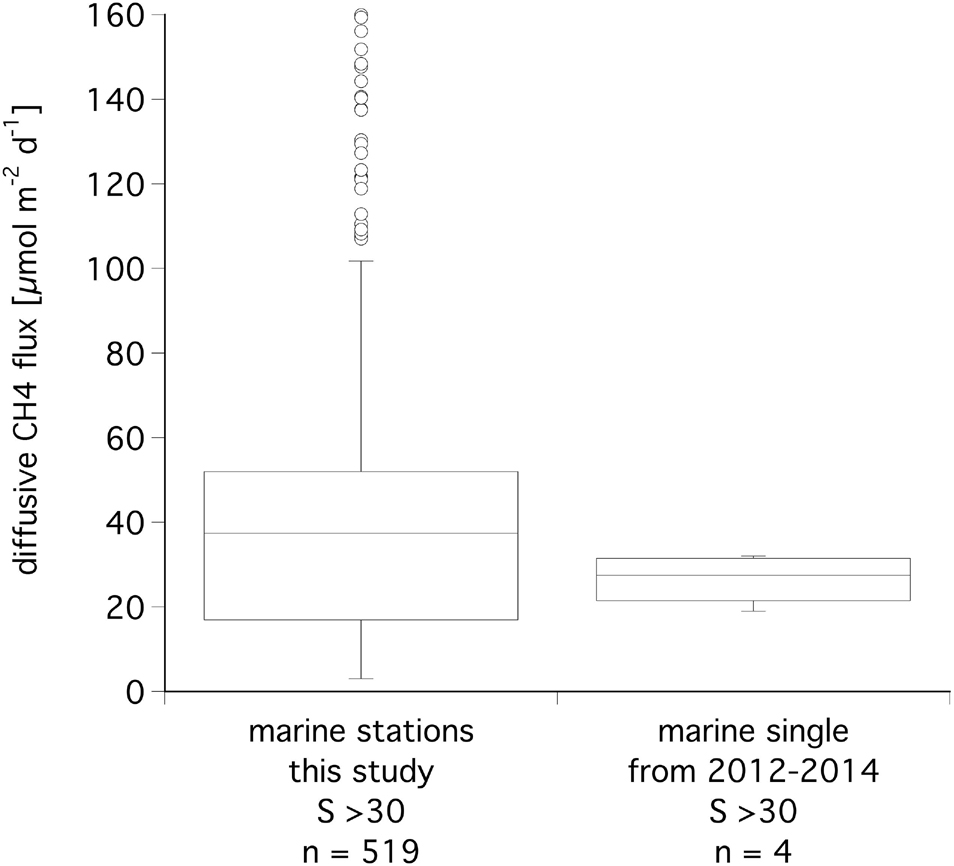
Figure 7. Range of data on diffusive methane flux at marine stations from this study and from previous years. The boxes enclose 50% of the data, the median is shown as a line. The upper and lower limit of the box (upper and lower quartile, UQ, LQ) indicate values which are halfway between the median and the largest/smallest data value. The difference between these limits is defined as IQD. Outliers are defined as values which are > UQ + (1.5 * IQD) or < LQ + (1.5 * IQD).

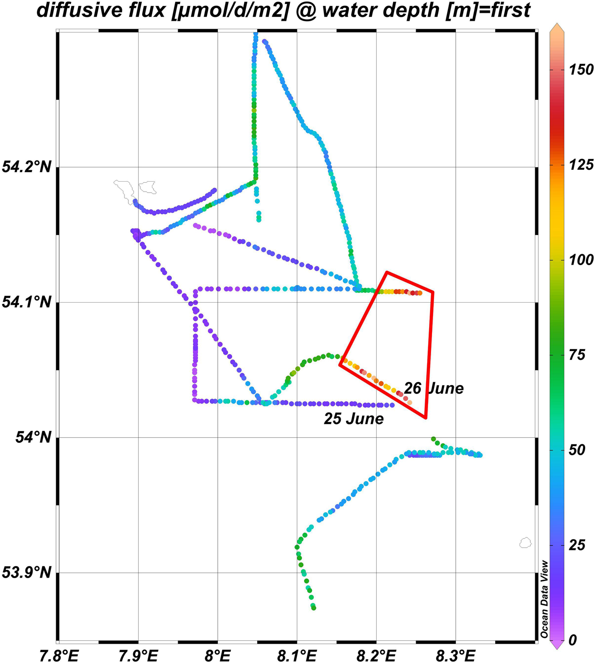
Figure 8. Close up for the diffusive methane flux only in the marine area (S > 30), red polygon indicated the area of increased flux.

In Figure 8, the diffusive methane flux in the marine area shows that these outliers were all located in one area (red rectangle). On June 25, 2019, the RV Uthörn passed at approximately 1 km south of this area, and only low methane fluxes were recorded. However, 23 h later and 1 km north of the previous cruise track, an area with significantly higher methane flux was observed. The original data revealed that the combination of elevated methane concentrations and increased wind speed in this area at that time were the reasons for the increased diffusive methane flux.

Conclusion

Previous studies have not always presented clear explanations for the observed patterns of dissolved methane or report low correlations with inconsistent patterns. This study used a higher spatial resolution to better clarify these aspects.

The overall pattern of methane distribution in the coastal North Sea is that of a dilution of riverine water with marine water. But the methane load of the rivers is also strongly influenced by their discharge. In this context the Elbe River had much stronger impact than the Weser River. However, anomalies from single water parameters also revealed strong correlations of turbidity, oxygen, and water mass origin with CH₄ concentrations. Nevertheless, these single parameters were not consistent over time. At certain times or locations, we observed highly significant correlations between methane and oxygen or turbidity. However, this was not valid for the entire cruise. Within 24 h, the observed relationships and explicable patterns disappeared at a certain location. A similar patchy and temporary dynamic distribution of methane in surface waters has also been described by Joung et al. (2020).

The question remains, how long an elevated methane concentration has to last or how wide has an area of elevated methane concentrations to be to be recognized as significant pattern? This depends on the spatial and temporal resolution of the sampling and the scientific focus (Fischer et al. submitted). Our study with a spatial resolution of 200–300 m and temporal resolution of 1 min indicates that there are additional significant small-scale patterns not yet understood.

The diffusive methane flux from surface water is the most important factor affecting the role of methane as a greenhouse gas. This study shows that high spatial resolution is necessary to better estimate the coastal methane flux. Even though the difference between average diffusive flux based on continuous measurements and single point measurements was not significant, we could detect anomalies with increased fluxes. These findings are crucial to determine diffusive methane flux budgets more accurately by relating surface water concentrations to atmospheric concentrations. The combination of increased methane concentrations and increased wind speed resulted in a substantial spatially and temporally restricted increase in the diffusive methane flux. Therefore, the improved temporal and spatial resolution of methane measurements provided a more accurate estimation of coastal methane fluxes.

Data Availability Statement

All unprocessed data are available in the O2A database. Processed data as outlined in the Materials and Methods section can be found in the Pangea data base; for 2018 at https://doi.pangaea.de/10.1594/PANGAEA.934404 and for 2019 at https://doi.pangaea.de/10.1594/PANGAEA.935354.

Author Contributions

IB processed the methane samples and data and wrote the manuscript. All authors participated in the planning and implementation of the cruises and contributed to the discussions, contributed to the manuscript, and approved the submitted version.

Funding

This study was part of the Helmholtz program Changing Earth, ST4.1: “Fluxes and transformation of energy and matter in and across compartments;” as well as the cross-topic activity MOSES (Modular Observation Solutions for Earth Systems).

Conflict of Interest

The authors declare that the research was conducted in the absence of any commercial or financial relationships that could be construed as a potential conflict of interest.

Publisher’s Note

All claims expressed in this article are solely those of the authors and do not necessarily represent those of their affiliated organizations, or those of the publisher, the editors and the reviewers. Any product that may be evaluated in this article, or claim that may be made by its manufacturer, is not guaranteed or endorsed by the publisher.

Acknowledgments

We thank the crew of the RV Ludwig Prandtl and RV Uthörn for their support, especially for allowing a flexible cruise planning. We would also like to thank Housam Dibeh from Hereon, who developed the web interface for the drift model we applied in our analysis. We are grateful to Iris Krippenstapel (River Basin Commission Weser) for the fruitful discussions on the Weser water flow.

Supplementary Material

The Supplementary Material for this article can be found online at: https://www.frontiersin.org/articles/10.3389/fmars.2021.728308/full#supplementary-material

Supplementary Figure S1 | Salinity of surface water (both days, both ships).

Supplementary Figure S2 | Dilution of Elbe water 25 June. The boxes indicate the riverine and marine part.

Supplementary Figure S3 | Delta 13-C of CH4 versus the inverse CH4 concentration (Keeling plot). Circles indicate data from RV Uthörn, squares data from RV Prandtl. Red triangles indicate riverine stations, their location is shown in Figure 3. The regression line is based on all data.

Supplementary Figure S4 | Location of stations above E1, E2) and on (W1, W2) the dilution line for Weser water with marine endmember on 26th June.

Supplementary Figure S5 | The diffusive methane flux in the marine area (solid line with S > 30), in the estuarine area (dashed line with 25.1 < S < 29.9) and riverine area (dotted line with S > 25).

Supplementary Figure S6 | Discharge of the rivers Elbe (at Neu Darchau, in black) and Weser (at Intschede, in blue) in 2019. Vertical line indicates the date of our cruise and the dotted line 3 weeks previously.

Footnotes

1. ^ https://www.elbe-datenportal.de
2. ^ https://datenbank.fgg-weser.de
3. ^ https://www.ufz.de/moses/
4. ^ https://doi.pangaea.de/10.1594/PANGAEA.934404
5. ^ http://www.esrl.noaa.gov/gmd/dv/iadv/
6. ^ https://www.dwd.de
7. ^ https://dashboard.awi.de/data-xxl/overview.jsp
8. ^ https://www.fgg-weser.de/
9. ^ https://hcdc.hereon.de/drift-now/
10. ^ https://www.bsh.de/EN/TOPICS/Operational_models/operational_models_node.html

References

Alin, S. R., de Fátima, F. L., Rasera, M., Salimon, C. I., Richey, J. E., Holtgrieve, G. W., et al. (2011). Physical controls on carbon dioxide transfer velocity and flux in low-gradient river systems and implications for regional carbon budgets. J. Geophys. Res. G 116:G01009. doi: 10.1029/2010jg001398
ARGE Weser. (1982). Weserlastplan. Arbeitsgemeinschaft der Länder zur Reinhaltung der Weser. Bremen: ARGE Weser.
Aromokeye, D. A., Kulkarni, A. C., Elvert, M., Wegener, G., Henkel, S., Coffinet, S., et al. (2020). Rates and microbial players of iron-driven anaerobic oxidation of methane in methanic marine sediments. Front. Microbiol. 10:3041. doi: 10.3389/fmicb.2019.03041
Becker, G. A., Giese, H., Isert, K., König, P., Langenberg, H., Pohlmann, T., et al. (1999). Mesoscale structures, fluxes and water mass variability in the German Bight as exemplified in the KUSTOS-experiments and numerical models. German J. Hydrogr. 51, 55–179. doi: 10.1007/BF02764173
Borges, A. V., and Abril, G. (2012). “Carbon dioxide and methane dynamics in estuaries,” in Treatise on Estuarine and Coastal Science, ed. E. Wolanski (Waltham: Academic Press), 119–161.
Borges, A. V., Royer, C., Martin, J. L., Champenois, W., and Gypens, N. (2019). Response of marine methane dissolved concentrations and emissions in the Southern North Sea to the European 2018 heatwave. Continental Shelf Res. 4:190. doi: 10.1016/j.csr.2019.104004
Borges, A. V., Speeckaert, G.l., Champenois, W., Scranton, M. I, and Gypens, N. (2017). Productivity and temperature as drivers of seasonal and spatial variations of dissolved methane in the southern bight of the North Sea. Ecosystems 21, 583–599. doi: 10.1007/s10021-017-0171-7
Bussmann, I., Brix, H., Flöser, G., Ködel, U., and Fischer, P. (2021). Dissolved methane, diffusive methane flux and underway oceanography of Stern 2 cruises in June 2019, in the southern German Bight with Elbe and Weser Estuary. PANGAEA. Available online at: https://doi.pangaea.de/10.1594/PANGAEA.935354
Bussmann, I., Brix, H., Mario Esposito, Friedrich, M., and Fischer, P. (2020). “The MOSES Sternfahrt Expeditions of the Research Vessels LITTORINA, LUDWIG PRANDTL, MYA II, UTHÖRN to the inner German Bight in 2019,” in Reports on Polar and Marine Research, ed. H. Bornemann (Bremerhaven: Alfred Wegener Institut).
Bussmann, I., Hackbusch, S., and Warnstedt, J. (2019). Methane Concentrations and Methane Oxidation Rates from Jan 2013 - Nov 2014 in the Elbe Estuary, From Hamburg to Helgoland. Germany: PANGAEA, doi: 10.1594/PANGAEA.897351
Bussmann, I., Osudar, R., and Matousu, A. (2014). Methane Concentrations and Methane Oxidation Rates From Oct 2010 - Jun 2012 on a Transect from Cuxhaven to Helgoland. Germany: PANGAEA.
Callies, U. (2021). Sensitive dependence of trajectories on tracer seeding positions – coherent structures in German Bight backward drift simulations. Ocean Sci. 17, 527–541. doi: 10.5194/os-17-527-2021
Farías, L., Tenorio, S., Sanzana, K., and Faundez, J. (2021a). Temporal methane variability in the water column of an area of seasonal coastal upwelling: A study based on a 12 year time series. Progr. Oceanogr. 195:102589. doi: 10.1016/j.pocean.2021.102589
Farías, L., Troncoso, M., Sanzana, K., Verdugo, J., and Masotti, I. (2021b). Spatial distribution of dissolved methane over extreme oceanographic gradients in the subtropical eastern south Pacific (17° to 37°S). J. Geophys. Res 126:e2020JC016925. doi: 10.1029/2020JC016925
Grunwald, M., Dellwig, O., Beck, M., Dippner, J. W., Freund, J. A., Kohlmeier, C., et al. (2009). Methane in the southern North Sea: sources, spatial distribution and budgets. Estuar. Coastal Shelf Sci. 81, 445–456. doi: 10.1016/j.ecss.2008.11.021
Hackbusch, S., Wichels, A., and Bussmann, I. (2019). Abundance, activity and diversity of methanotrophic bacteria in the Elbe Estuary and southern North Sea. Aquat. Microb. Ecol. 83, 35–48. doi: 10.3354/ame01899
IPCC, Ciais, P., Sabine, C., Bala, G., Bopp, L., Brovkin, V., et al. (2013). “Carbon and other biogeochemical cycles,” in Climate Change 2013: The Physical Science Basis. Contribution of Working Group I to the Fifth Assessment Report of the Intergovernmental Panel on Climate Change, eds T. F. Stocker, D. Qin, G.-K. Plattner, M. Tignor, S. K. Allen, J. Boschung, et al. (Cambridge: Cambridge University Press).
Jacques, C., Gkritzalis, T., Tison, J.-L., Hartley, T., van der Veen, C., Röckmann, T., et al. (2020). Carbon and hydrogen isotope signatures of dissolved methane in the Scheldt Estuary. Estuar. Coasts 44, 137–146. doi: 10.1007/s12237-020-00768-3
Jansson, P., Triest, J., Grilli, R., Ferré, B., Silyakova, A., Mienert, J., et al. (2019). High-resolution underwater laser spectrometer sensing provides new insights into methane distribution at an Arctic seepage site. Ocean Sci. 15, 1055–1069. doi: 10.5194/os-15-1055-2019
Joung, D., Leonte, M., Valentine, D. L., Sparrow, K. J., Weber, T., and Kessler, J. D. (2020). Radiocarbon in marine methane reveals patchy impact of seeps on surface waters. Geophys. Res. Lett. 47:e2020GL089516. doi: 10.1029/2020GL089516
Karl, D. M., Beversdorf, L., Bjoerkman, K. M., Church, M. J., Martinez, A., and DeLong, E. F. (2008). Aerobic production of methane in the sea. Nat. Geosci. 1, 473–478.
Klintzsch, T., Langer, G., Wieland, A., Geisinger, H., Lenhart, K., Nehrke, G., et al. (2020). Effects of temperature and light on methane production of widespread marine phytoplankton. J. Geophys. Res. 125:e2020JG005793. doi: 10.1029/2020JG005793
Krämer, K., Holler, P., Herbst, G., Bratek, A., Ahmerkamp, S., Neumann, A., et al. (2017). Abrupt emergence of a large pockmark field in the German Bight, southeastern North Sea. Scient. Rep. 7:5150. doi: 10.1038/s41598-017-05536-1
Le Guitton, M., Soetaert, K., Sinninghe Damsté, J. S., and Middelburg, J. J. (2017). A seasonal study of particulate organic matter composition and quality along an offshore transect in the southern North Sea. Estuar. Coast. Shelf Sci. 188, 1–11. doi: 10.1016/j.ecss.2017.02.002
Lenhart, K., Klintzsch, T., Langer, G., Nehrke, G., Bunge, M., Schnell, S., et al. (2016). Evidence for methane production by the marine algae Emiliania huxleyi. Biogeosciences 13, 3163–3174. doi: 10.5194/bg-13-3163-2016
Li, Y., Zhan, L., Chen, L., Zhang, J., Wu, M., and Liu, J. (2021). Spatial and temporal patterns of methane and its influencing factors in the Jiulong River estuary, southeastern China. Mar. Chem. 228:909. doi: 10.1016/j.marchem.2020.103909
Lindeman, R. H., Merenda, P. F., and Gold, R. Z. (1980). Introduction to Bivariate and Multivariate Analysis. Glenview IL: Scott.
Magen, C., Lapham, L. L., Pohlman, J. W., Marshall, K., Bosman, S., Casso, M., et al. (2014). A simple headspace equilibration method for measuring dissolved methane. Limnol. Oceanogr.: Methods 12, 637–650. doi: 10.4319/lom.2014.12.637
Manning, C. C., Preston, V. L., Jones, S. F., Michel, A. P. M., Nicholson, D. P., Duke, P. J., et al. (2020). River inflow dominates methane emissions in an Arctic coastal system. Geophys. Res. Lett. 47:e2020GL087669. doi: 10.1029/2020GL087669
Matousu, A., Osudar, R., Simek, K., and Bussmann, I. (2017). Methane distribution and methane oxidation in the water column of the Elbe estuary. Germany Aquatic Sci. 79, 443–458. doi: 10.1007/s00027-016-0509-9
Mau, S., Gentz, T., Körber, J. H., Torres, M. E., Römer, M., Sahling, H., et al. (2015). Seasonal methane accumulation and release from a gas emission site in the central North Sea. Biogeosciences 12, 5261–5276. doi: 10.5194/bg-12-5261-2015
Mordhorst, J. (1981). Müllkippe Nordsee?: Alles über Ölpest und Billigflaggen, über Industrieabfälle und Verklappung, über Umweltverschmutzung und die bedrohte Natur. Hamburg: Maritim.
Myllykangas, J.-P., Hietanen, S., and Jilbert, T. (2020). Legacy effects of eutrophication on modern methane dyanmics in a boreal estuary. Estuar. Coasts 43, 189–206. doi: 10.1007/s12237-019-00677-0
Nauw, J., de Haas, H., and Rehder, G. (2015). A review of oceanographic and meteorological controls on the North Sea circulation and hydrodynamics with a view to the fate of North Sea methane from well site 22/4b and other seabed sources. Mar. Petrol. Geol. 68, 861–882. doi: 10.1016/j.marpetgeo.2015.08.007
Nightingale, P. D., Malin, G., Law, C. S., Watson, A. J., Liss, P. S., Liddicoat, M. I., et al. (2000). In situ evaluation of air-sea gas exchange parameterizations using novel conservative and volatile tracers. Global Biogeochem. Cycles 14, 373–387. doi: 10.1029/1999GB900091
Osudar, R., Matoušů, A., Alawi, M., Wagner, D., and Bussmann, I. (2015). Environmental factors affecting methane distribution and bacterial methane oxidation in the German Bight (North Sea). Estuar. Coast. Shelf Sci. 160, 10–21. doi: 10.1016/j.ecss.2015.03.028
Petersen, W. (2014). FerryBox systems: State-of-the-art in Europe and future development. J. Mar. Syst. 140, 4–12. doi: 10.1016/j.jmarsys.2014.07.003
Pfeiffer-Herbert, A. S., Prahl, F. G., Hales, B., Lerczak, J. A., Pierce, S. D., and Levine, M. D. (2016). High resolution sampling of methane transport in the Columbia River near-field plume: Implications for sources and sinks in a river-dominated estuary. Limnol. Oceanogr. 61, S204–S220. doi: 10.1002/lno.10221
Repeta, D. J., Ferrón, S., Sosa, O. A., Johnson, C. G., Repeta, L. D., Acker, M., et al. (2016). Marine methane paradox explained by bacterial degradation of dissolved organic matter. Nat. Geosci. 9, 884–887. doi: 10.1038/ngeo2837
Römer, M., Wenau, S., Mau, S., Veloso, M., Greinert, J., Schlüter, M., et al. (2017). Assessing marine gas emission activity and contribution to the atmospheric methane inventory: A multidisciplinary approach from the Dutch Dogger Bank seep area (North Sea). Geochem. Geophys. Geosyst. 18, 2617–2633. doi: 10.1002/2017GC006995
Røy, H., Jae, S. L., Jansen, S., and De Beer, D. (2008). Tide-driven deep pore-water flow in intertidal sand flats. Limnol. Oceanogr. 53, 1521–1530.
Saunois, M., Bousquet, P., Poulter, B., Peregon, A., Ciais, P., Canadell, J. G., et al. (2016). The global methane budget 2000–2012. Earth Syst. Sci. Data 8, 697–751. doi: 10.5194/essd-8-697-2016
Saunois, M., Stavert, A. R., Poulter, B., Bousquet, P., Canadell, J. G., Jackson, R. B., et al. (2020). The Global Methane Budget 2000–2017. Earth Syst. Sci. Data 12, 1561–1623. doi: 10.5194/essd-12-1561-2020
Schilder, J., Bastviken, D., van Hardenbroek, M., Kankaala, P., Rinta, P., Stötter, T., et al. (2013). Spatial heterogeneity and lake morphology affect diffusive greenhouse gas emission estimates of lakes. Geophys. Res. Lett. 40, 5752–5756. doi: 10.1002/2013GL057669
Schmale, O., Wäge, J., Mohrholz, V., Wasmund, N., Gräwe, U., Rehder, G., et al. (2018). The contribution of zooplankton to methane supersaturation in the oxygenated upper waters of the central Baltic Sea. Limnol. Oceanogr. 63, 412–430. doi: 10.1002/lno.10640
Schneider, B., Gülzow, W., Sadkowiak, B., and Rehder, G. (2014). Detecting sinks and sources of CO2 and CH4 by ferrybox-based measurements in the Baltic Sea: Three case studies. J. Mar. Syst. 140, 13–25. doi: 10.1016/j.jmarsys.2014.03.014
Schuchardt, B., Haesloop, U., and Schirmer, M. (1993). The tidal freshwater reach of the Weser estuary: Riverine or estuarine? Netherl. J. Aquat. Ecol. 27, 215–226. doi: 10.1007/BF02334785
Schwichtenberg, F., Pätsch, J., Böttcher, M. E., Thomas, H., Winde, V., and Emeis, K. C. (2020). The impact of intertidal areas on the carbonate system of the southern North Sea. Biogeosciences 17, 4223–4245. doi: 10.5194/bg-17-4223-2020
Sierra, A., Jiménez-López, D., Ortega, T., Gómez-Parra, A., and Forja, J. (2020). Factors controlling the variability and emissions of greenhouse gases (CO2, CH4 and N2O) in three estuaries of the Southern Iberian Atlantic Basin during July 2017. Mar. Chem. 226:103867. doi: 10.1016/j.marchem.2020.103867
Striegl, R. G., Dornblaser, M. M., McDonald, C. P., Rover, J. R., and Stets, E. G. (2012). Carbon dioxide and methane emissions from the Yukon River system. Glob. Biogeochem. Cycles 26:GB0E05. doi: 10.1029/2012GB004306
Teeling, H., Fuchs, B. M., Bennke, C. M., Krüger, K., Chafee, M., Kappelmann, L., et al. (2016). Recurring patterns in bacterioplankton dynamics during coastal spring algae blooms. eLife 5:e1188. doi: 10.7554/eLife.11888
Trifunovic, B., Vázquez-Lule, A., Capooci, M., Seyfferth, A. L., Moffat, C., and Vargas, R. (2020). Carbon dioxide and methane emission from temperate salt marsh tidal creek. Biogeosciences 125:558. doi: 10.1029/2019JG005558
Upstill-Goddard, R. C., and Barnes, J. (2016). Methane emissions from UK estuaries: Re-evaluating the estuarine source of tropospheric methane from Europe. Mar. Chem. 180, 14–23. doi: 10.1016/j.marchem.2016.01.010
van Beusekom, J. E. E., Brockmann, U. H., Hesse, K.-J., Hickel, W., Poremba, K., and Tillmann, U. (1999). The importance of sediments in the transformation and turnover of nutrients and organic matter in the Wadden Sea and German Bight. German J. Hydrogr. 51, 245–266.
Vielstädte, L., Haeckel, M., Karstens, J., Linke, P., Schmidt, M., Steinle, L., et al. (2017). Shallow gas migration along hydrocabon wells - an unconsidered, anthropogenic source of biogenic methane in the North Sea. Environ. Sci. Technol. 51, 10262–10268. doi: 10.1021/acs.est.7b02732
Wanninkhof, R. (2014). Relationship between wind speed and gas exchange over the ocean revisited. Limnol. Oceanogr. 12, 351–362. doi: 10.4319/lom.2014.12.351
Wanninkhof, R., Asher, W. E., Ho, D. T., Sweeney, C. S., and McGillis, W. R. (2009). Advances in quantifying air-sea gas exchange and environmental forcing. Annu. Rev. Mar. Sci. 1, 213–244. doi: 10.1146/annurev.marine.010908.163742
Weber, T., Wiseman, N. A., and Kock, A. (2019). Global ocean methane emissions dominated by shallow coastal waters. Nat. Commun. 10:4584. doi: 10.1038/s41467-019-12541-7
Wells, N. S., Chen, J. J., Maher, D. T., Huang, P., Erler, D. V., Hipsey, M., et al. (2020). Changing sediment and surface water processes increase CH4 emissions from human-impacted estuaries. Geochim. Cosmochim. Acta 280, 130–147. doi: 10.1016/j.gca.2020.04.020
Wiesenburg, D. A., and Guinasso, N. L. (1979). Equilibrium solubilities of methane, carbon monoxide and hydrogen in water and sea water. J. Chem. Eng. Data 24, 356–360.
Winkler, H. (2019). High resolution methane measurements and impacts of environmental factors on the methane distribution in the Elbe Estuary, Austria, Master Thesis of the University of Vienna.
Wu, C. S., Røy, H., and de Beer, D. (2015). Methanogenesis in sediments of an intertidal sand flat in the Wadden Sea. Estuar. Coast. Shelf Sci. 164, 39–45. doi: 10.1016/j.ecss.2015.06.031
Yang, M., Bell, T. G., Brown, I. J., Fishwick, J. R., Kitidis, V., Nightingale, P. D., et al. (2019). Insights from year-long measurements of air–water CH4 and CO2 exchange in a coastal environment. Biogeosciences 16, 961–978. doi: 10.5194/bg-16-961-2019
Keywords: dissolved methane, North Sea, high temporal resolution, high spatial resolution, diffusive methane flux
Citation: Bussmann I, Brix H, Flöser G, Ködel U and Fischer P (2021) Detailed Patterns of Methane Distribution in the German Bight. Front. Mar. Sci. 8:728308. doi: 10.3389/fmars.2021.728308
Received: 22 June 2021; Accepted: 23 August 2021;
Published: 17 September 2021.
Edited by:
Christian Lønborg, Aarhus University, DenmarkReviewed by:
Tom Jilbert, University of Helsinki, FinlandKui Wang, Zhejiang University, China
Anna Pauline Miranda Michel, Woods Hole Oceanographic Institution, United States
Copyright © 2021 Bussmann, Brix, Flöser, Ködel and Fischer. This is an open-access article distributed under the terms of the Creative Commons Attribution License (CC BY). The use, distribution or reproduction in other forums is permitted, provided the original author(s) and the copyright owner(s) are credited and that the original publication in this journal is cited, in accordance with accepted academic practice. No use, distribution or reproduction is permitted which does not comply with these terms.
*Correspondence: Ingeborg Bussmann, Ingeborg.bussmann@awi.de