Roles of Iron Limitation in Phytoplankton Dynamics in the Western and Eastern Subarctic Pacific

Introduction

Marine phytoplankton have been found to be a key component in marine ecosystems and the global carbon cycle (Fasham, 2003). They contribute more than 45% of the global photosynthetic net primary production with only 1% of the photosynthetic biomass (Simon et al., 2009). Production is especially high at high latitudes; the phytoplankton dynamics in these kinds of regions make them the most productive, seasonally dynamic, and rapidly changing ecosystems across global oceans (Huston and Wolverton, 2009; Behrenfeld et al., 2017). In the majority of high-latitude seas, e.g., the subarctic Pacific Ocean, iron (Fe) is thought to be the primary limiting nutrient for biological production (Miller et al., 1991; Moore et al., 2004). Furthermore, variability in Fe bioavailability is also important for marine ecosystems because it affects the phytoplankton dynamics in these regions.

The subarctic Pacific Ocean has two major time-series stations that are associated with each of the gyres. Station Papa (Stn. Papa), which is associated with Biogeochemical-Argo (BGC-Argo) observations from 2008 to 2015 and more than 60 years of cruise observations, is located at 50°N and 145°W on the southeastern edge of the Alaska Gyre in the eastern subarctic Pacific (Freeland, 2007). On the other hand, observations at Station K2 (Stn. K2, 47°N, 160°E), which is at the center of the western subarctic gyre, have been carried out with a tethered mooring system and repetitive shipboard observations since 2001 (Honda and Watanabe, 2007). Previous observational studies have revealed the similarities between the seasonal cycles in the physical environments of these two stations, e.g., the mixed layer depth (MLD) is much shallower in the summer (<30 m) than in the winter (>100 m) (Harrison et al., 2004; Fujiki et al., 2014; Plant et al., 2016). Furthermore, the strong winter mixing at each station also entrains nitrate and silicate into the mixed layer, resulting in an increase in their concentrations in the winter. Both the western and the eastern subarctic Pacific are characterized as high-nitrate, low-chlorophyll (HNLC) regions. In these regions, the surface nitrate concentration always remains sufficient for phytoplankton growth, although its value decreases from winter to summer, as nitrate is consumed by these phytoplankton (Harrison et al., 1999). However, their chlorophyll concentrations show significant differences in seasonal variability. For example, phytoplankton bloom occurs two times per year at Stn. K2, with chlorophyll peaks (>1 mg m⁻³) in spring to early summer and early autumn; at Stn. Papa, the seasonal variability of chlorophyll is weak (0.2–0.6 mg m⁻³), but concentrations are slightly higher in late summer (Mochizuki et al., 2002; Pena and Varela, 2007; Matsumoto et al., 2014). The mechanisms underlying these marine ecosystems on the two sides of the subarctic Pacific have been actively investigated, and they have been found to be related to the differences in Fe bioavailability in explored in several studies (Banse and English, 1999; Harrison et al., 1999; Fujii et al., 2007; Nishioka et al., 2021).

Previous shipboard Fe-enrichment experiments in the western and eastern subarctic Pacific have shown that the addition of dissolved iron, which has a size < 0.2 or 0.45 μm (Gledhill and Buck, 2012), to in situ water significantly increased nutrient utilization and led to an enhancement in the concentration of chlorophyll (Martin and Fitzwater, 1988; Boyd et al., 1996; Tsuda et al., 2003; Marchetti et al., 2006a). This indicates that bioavailable Fe (BFe), which can be directly accessed by phytoplankton (Nishioka et al., 2021), limits phytoplankton growth, especially diatom growth, in these two regions, and that BFe limitation was also the cause of the HNLC conditions in the subarctic Pacific (Martin et al., 1991; Harrison et al., 2004; Marchetti et al., 2006b). In the eastern subarctic Pacific, the dissolved Fe concentration and the bioavailability of Fe are both lower than those in the western subarctic Pacific (Harrison et al., 2004; Nishioka et al., 2007; Kondo et al., 2021). The corresponding phytoplankton group in the eastern subarctic Pacific is also persistently dominated by small phytoplankton, as the growth of diatoms is limited by Fe (Boyd and Harrison, 1999; Yang et al., 2018). In contrast, the small phytoplankton at Stn. Papa, which is less affected by BFe limitation, have been considered to be top-down controlled by grazing by zooplankton, particularly by microzooplankton (Miller et al., 1991; Harrison, 2002). In the western subarctic Pacific, previous observations have consistently shown that diatoms are the dominant phytoplankton group during bloom periods in the spring and early summer (Obayashi et al., 2001; Imai et al., 2002). With the deficiency of BFe in the summer, the diatom biomass gradually decreased, but the small phytoplankton biomass increased and came to dominate the phytoplankton group during the bloom period in early autumn (Fujiki et al., 2009, 2014; Nishioka et al., 2011). Furthermore, a previous study has shown that the small phytoplankton bloom in autumn is also related to reductions in microzooplankton grazing pressure in small phytoplankton (Matsumoto et al., 2014). Therefore, the major difference between the western and eastern subarctic Pacific marine ecosystems, which is the occurrence of seasonal phytoplankton blooms, depends on the availability of Fe for different phytoplankton and is simultaneously influenced by zooplankton grazing. However, quantitatively evaluating the relative roles of BFe in the seasonal variability of phytoplankton growth in these two regions is challenging, as observational data on Fe are scarce and there are few time-series datasets available. Although some marine ecosystem models have been developed to investigate the role of Fe in these two subarctic Pacific ecosystems, the associated studies have usually focused on only one region (Denman and Pena, 1999; Pena, 2003; Shigemitsu et al., 2012) or have not incorporated the cycle of Fe into their models (Fujii et al., 2007).

Because of the importance of Fe in regulating phytoplankton growth in the subarctic Pacific, the various sources of dissolved Fe have been actively studied. The dissolved Fe in the upper ocean comes mainly from atmospheric dust (Jickells et al., 2005), vertical diffusion (Nishioka et al., 2020), horizontal transport via recirculation and eddies (Johnson et al., 2005), and the remineralization of sinking particulates (Lamborg et al., 2008). Although the magnitudes of the contributions of various Fe sources the upper ocean of the subarctic Pacific are still debated (Tagliabue et al., 2014; Ito and Shi, 2016; Nishioka and Obata, 2017; Nishioka et al., 2020), there have been a series of observations and numerical models confirming that Fe addition by atmospheric dust plays an important role in controlling phytoplankton biomass and primary production (PP), especially in HNLC regions (Boyd et al., 1998; Bishop et al., 2002; Jickells et al., 2005; Nishioka et al., 2021). Additionally, the dissolved Fe supply from atmospheric dust transported to the western subarctic Pacific is much higher than that transported to the eastern subarctic Pacific (Nishioka et al., 2003), because the Gobi Desert, a major dust source, is closer to the western subarctic Pacific and prevailing winds favor the transport of dust from this region into the ocean (Boyd et al., 1998; Luo et al., 2008). These conditions result in the contributions of atmospheric deposition to the BFe in the upper ocean differing between the two regions (Krishnamurthy et al., 2010). Furthermore, previous studies have shown that an increase in human activities can cause more dissolved Fe from atmospheric dust to enter the ocean; this is particularly true for Fe from combustion sources, which has higher bioavailability in the upper ocean (Krishnamurthy et al., 2009; Mahowald et al., 2009). Additionally, an increase in external dissolved Fe deposition from atmospheric dust would drive different responses in the phytoplankton in the western and eastern subarctic Pacific. However, the influence of changes in dust sources on the marine ecosystem in the upper ocean of the subarctic Pacific has rarely been investigated in previous studies.

In this study, a one-dimensional physical-biological model that included the Fe cycle was applied to compare the influence of bioavailable Fe on the phytoplankton dynamics of Stn. K2 and Stn. Papa in the western and eastern subarctic Pacific, respectively. To evaluate the performance of this model in reproducing the physical and biogeochemical processes at Stn. K2 and Stn. Papa, the simulated results were validated with observational data from BGC-Argo and cruise observations. This study can help in understanding the role of Fe in the phytoplankton dynamics of the western and eastern subarctic Pacific and the responses of phytoplankton in projected future scenarios.

Model and Data

One-Dimensional Coupled Model

Two one-dimensional physical–biogeochemical (Ma et al., 2019) coupled models incorporating the Fe cycle (Xiu and Chai, 2021) were applied to the locations of Stn. K2 in the western subarctic Pacific and Stn. Papa in the eastern subarctic Pacific. Both sites selected for modeling are located in the deep basin of the North Pacific, far from the continental shelf, with bottom depths of >5,000 m at Stn. K2 and >4,000 m at Stn. Papa. The physical model was based on the Regional Ocean Modeling System (ROMS) and ignored lateral processes. Furthermore, the turbulent vertical mixing in this study was based on the non-local K profile parameterization (KPP; Large et al., 1994). In these regions, vertical diffusion has a stronger effect on phytoplankton dynamics than other factors, and it was simulated in a previous 1D model without advection or horizontal diffusion processes (Denman and Pena, 1999; Fujii et al., 2007; Sasai et al., 2016). Thus, the model used in this study included 300 layers in the vertical direction that extended to 5,000 m in depth at Stn. K2 and to 4,000 m at Stn. Papa, with a finer resolution near the surface.

The biogeochemical model used in this study was based on a newly developed carbon silicate nitrate ecosystem-Fe (CoSiNE-Fe) model (Xiu and Chai, 2021). It included two phytoplankton groups [picoplankton (S₁, Chl₁, S_1Fe) and diatoms (S₂, Chl₂, S_2Fe)], two zooplankton groups [microzooplankton (ZZ₁, ZZ_1Fe) and mesozooplankton (ZZ₂, ZZ_2Fe)], two size classes of particulate organic nitrogen [small (S_PON, S_PFe) and large (L_PON, L_PFe)], two size classes of biogenic silica [small (S_bSi) and large (L_bSi)], four inorganic nutrients [nitrate (NO₃), ammonium (NH₄), phosphate (PO₄), and silicate (SiOH₄)], dissolved oxygen (DO), two carbonate variables [dissolved inorganic carbon (DIC) and total alkalinity (TALK)], three size classes of dust particles [dust particles (Part_Dust, Dust_Fe), large lithogenic particles (Lith_PartL, Lith_LFe), small lithogenic particles (Lith_PartS, Lith_SFe)], soluble Fe (Fe_Sol), colloidal Fe (Fe_Col), strong and weak Fe ligands (Fe_LgS, Fe_LgW), and strong and weak ligands (Lg_S, Lg_W).

The Fe in particles can be transformed into colloidal Fe and soluble Fe through redissolution and photoreduction, respectively. Specifically, colloidal Fe is formed from soluble Fe and is removed from the dissolved pool through colloidal aggregation. Thus, in this study, bioavailable Fe included both soluble and ligand Fe, whereas colloidal Fe was assumed to not be directly accessible by phytoplankton (Jiang et al., 2013). Furthermore, the growth of small phytoplankton and diatoms depends on light, temperature, and nutrient availability. The losses of phytoplankton through biological processes occur because of mortality, aggregation, and zooplankton grazing. Consequently, the mortality and aggregation of phytoplankton and zooplankton form detritus, which is remineralized into the inorganic matter during sinking (Ma et al., 2019). In particular, microzooplankton graze on small phytoplankton, while mesozooplankton graze on diatoms, microzooplankton, and both large and small particulate organic nitrogen. With this, the seasonal vertical migration of mesozooplankton results in high biomass in the epipelagic layer during summer and in the mesopelagic layer during winter (Mackas and Tsuda, 1999). As a result, no diatoms or microzooplankton are grazed in winter, as mesozooplankton are absent from the upper ocean, and grazing initiates after spring (Kobari and Ikeda, 1999). These patterns were incorporated into the model. Additionally, some mesozooplankton overwintering without grazing was also included in the model, e.g., thresholds for mesozooplankton mortality mesozooplankton grazing on microzooplankton and diatoms were also applied. A similar effect of the seasonal vertical migration of mesozooplankton has also been considered in previous modeling studies (Kishi et al., 2001; Fujii et al., 2007). In this model, however, a photoacclimation assumption was included to improve the accuracy of chlorophyll simulation. Specifically, the ratio between chlorophyll and phytoplankton biomass varied (Fennel and Boss, 2003), and this ratio was parameterized following Ma et al. (2019). To simulate the marine ecosystems in both regions, the values of some parameters in the two models were made slightly different in order to reproduce the seasonal ecosystem variability. In particular, the species compositions of diatoms and small phytoplankton in the western and eastern subarctic Pacific differ (Timothy et al., 2013; Fujiki et al., 2014). The differences in the compositions of phytoplankton between the two regions also lead to variations in their adaptability to their environments, e.g., light and nutrients. As a result, the different photosynthesis parameters of phytoplankton, e.g., maximum growth rate of small phytoplankton, initial slope of P-I curve of small phytoplankton and diatom (Supplementary Table 1), used in the model were within a reasonable range. A similar approach has been applied in previous modeling studies to simulate marine ecosystems and compare phytoplankton dynamics between different regions (Fujii et al., 2005, 2007; Sasai et al., 2016).

The National Centers for Environmental Prediction (NCEP) reanalysis I data from 2001 to 2014 at Stn. K2 and Stn. Papa were extracted to produce six hourly forcings (Kalnay et al., 1996). The parameterizations of the selected air-sea fluxes were adopted from Ma et al. (2019). In addition, the forcing data file included the atmospheric deposition data (soluble Fe deposition and lithogenic particle deposition) from Chien et al. (2016), with both dust and non-dust sources. Because of the lack of real-time data, climatological seasonal deposition fluxes, which do not include episodic dust events, were used in the model in this study. The model was then initialized with the fields of the World Ocean Atlas 2018 (WOA18) (Garcia et al., 2018). The initial conditions for Fe variables, obtained from an updated version of the global Fe dataset (Tagliabue et al., 2012), were interpolated from the observed dissolved Fe profiles around Stn. K2 and Stn. Papa. The MLD was calculated as the depth at which the density was equal to the density at 10 m plus 0.03 kg m⁻³ (de Boyer Montégut, 2004). The averaged regulating factors (nutrients, temperature, and light), limiting nutrients (nitrogenous nutrients, phosphate, and bioavailable Fe), and the growth rates of the small phytoplankton and diatoms were individually calculated by vertical integration and then weighted and normalized to the corresponding phytoplankton biomass. The equation used is as follows:

where $\overline{rate}$ is the rate averaged within the water column, rate is the rate of biological activity of phytoplankton, S is the phytoplankton biomass, i is the layer of the model, and n is the total number of layers of the model. The method of vertical integration followed Fujii et al. (2005, 2007).

To evaluate the effect of an increase in dissolved Fe in atmospheric deposition, three cases were simulated to compare with the control run at Stn. K2 and Stn. Papa, respectively. These cases were forced with two (DFe Dep *2), three (DFe Dep *3), and four times (DFe Dep *4) with as much dissolved Fe in atmospheric deposition as in the control run between 2009 and 2013.

Cruise and Float Data

Shipboard observations were conducted during each season to facilitate the estimation of the seasonal variability at Stn. K2 between 2005 and 2013 (Matsumoto et al., 2014). Water samples were collected with a conductivity-temperature-depth (CTD) profiler system, with the surface samples being collected with a plastic bucket. The nutrient and chlorophyll concentrations of the samples were then measured. Since the cruise observations were conducted in different months during 2005–2013, the data for each month were combined to obtain a full seasonal cycle. The modeled results, which were averaged from 2005 to 2013, were compared with the observational data from cruises. A similar procedure was then applied to verify the accuracy of the models in a previous modeling study that was performed at Stn. K2 (Sasai et al., 2016).

Six BGC-Argo profiling floats [Autonomous Profiling Explorer (APEX) BioGeoChem, Teledyne Marine/Webb Research, North Falmouth, MA, United States] (BGC-Argo) were assembled at the University of Washington and deployed at Stn. Papa between August 2008 and June 2013 (Plant et al., 2016). In addition to temperature and salinity sensors, all the floats were equipped with in situ ultraviolet spectrophotometer (ISUS) optical nitrate sensors. Two floats (6400 and 7601) were equipped with WetLabs (WET Labs, Corvallis, Oregon, United States) FLBB optical chlorophyll fluorescence sensors, which measured chlorophyll concentrations (Haskell et al., 2020). To evaluate the performance of the model, the modeled sea surface temperature (SST), MLD, and surface nitrate (SNO₃) were compared with the six BGC-Argo observations from 2008 to 2014, and the modeled chlorophyll concentrations were compared with the two BGC-Argo observations from 2010 to 2013. The BGC-Argo observations were then applied when the floats were located <300 km from Stn. Papa to ensure that they were in a nearly identical biogeochemical environment (Pena and Varela, 2007). The sampling resolution was subsequently increased as the floats ascended from the parking depth, i.e., 1,000 m, to the shallowest sampling depth, i.e., 7 m, to capture greater variability in the surface waters. Specifically, the parameters were measured at 50-m intervals below 400 m, at 10-m intervals between 400 and 100 m, and at 5-m intervals above 100 m (Plant et al., 2016).

The observed dissolved Fe data from Tagliabue et al. (2012), Schallenberg et al. (2015), and Nishioka et al. (2020) were collected to validate the model. The dissolved Fe data in Tagliabue et al. (2012) were the GEOTRACES historical trace elements and their isotopes (TEI) data, and the observed dissolved Fe data is operationally defined as the Fe fraction that passes through a 0.2-μm and 0.4-μm filter. The data in Schallenberg et al. (2015) were operationally defined as the Fe fraction that passes through a 0.2-μm filter. Similarly, either a 0.22-μm Millipak filter (Millipore, Burlington, MA, United States) or a 0.2-μm Acropak capsule filter (PALL Corporation, Port Washington, New York, United States); was connected to a Niskin-X spigot (General Oceanics, Miami, Florida, United States) to measure the dissolved Fe (Nishioka et al., 2020).

Results

Comparison of Simulated Results With Observations

The simulated results at Stn. K2 (western subarctic Pacific region) and Stn. Papa (eastern subarctic Pacific region) were compared with corresponding observations (Figure 1). Specifically, the daily averaged data were applied over 9 years (2005–2013) at Stn. K2, while a time series of over 7 years, i.e., 2008–2014, was used at Stn. Papa. As a result, the simulated time series of SST and MLD clearly reproduced the seasonal cycles observed at both stations. At Stn. K2, the modeled SST decreased by approximately 2°C as the MLD deepened to a maximum depth of approximately 135 m in the winter, while the summer SST peak reached 12°C in September. The summer MLD reached its minimum of 15 m from June to August. Similarly, at Stn. Papa, the SST peaked (~14°C) in September and the MLD reached its minimum (~10 m) from June to August in the summer. In the winter, the modeled MLD reached its maximum (~120 m), associated with the minimum SST, but the winter SST was 3°C higher than that at Stn. K2. After 2013, the modeled SST was lower than the observations in the winter because a large, anomalously warm water patch (the “Blob”) appeared in the eastern Pacific because of horizontal advection, which was not considered in the 1D model (Bond et al., 2015). Since the “Blob” was a temporary event in winter after 2013–2016 (Yang et al., 2018), it had little influence on the normal seasonal cycles of marine ecosystems; thus, the model results from 2009 to 2013 were used in this study.

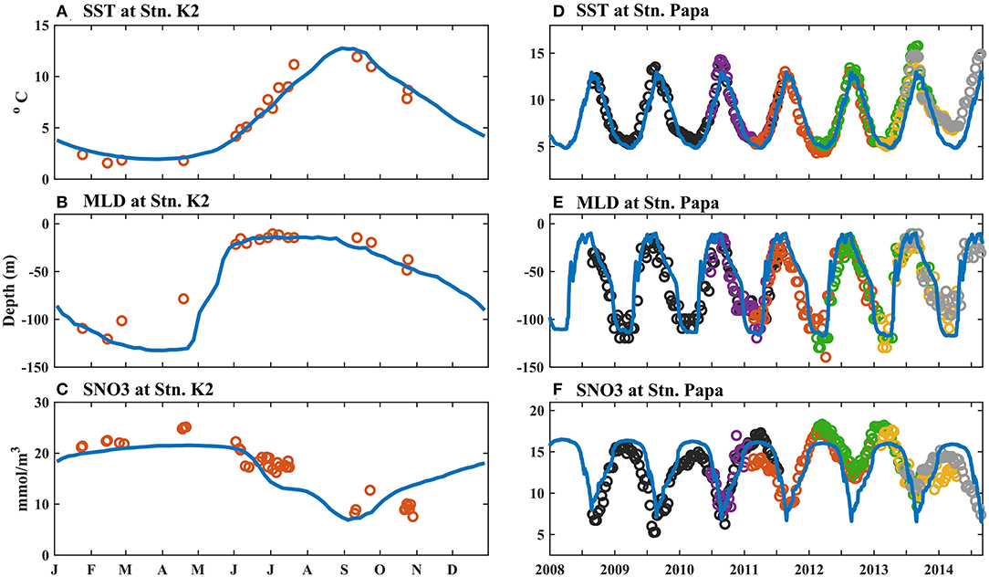
Figure 1. Comparison of sea surface temperature (SST; °C), mixed layer depth (MLD; m), and surface nitrate (SNO₃) between the model results (blue curve) and (A–C) cruise measurements during 2005–2013 (red hollow circle) at Station K2 (Stn. K2) and (D–F) Argo measurements during 2008–2014 (hollow circle) at Station Papa (Stn. Papa). The float numbers (and colors) (in D–F) are as follows: 5143 (black), 6400 (purple), 6972 (red), 7601 (green), 6881 (yellow), and 7641 (gray).

The biogeochemical components of the two ecosystems were also reproduced well by the model simulation (Figures 1C,F, 2, 3). Nutrient-rich water in the lower layer was supplied to the surface by enhanced mixing in the winter, leading to the highest simulated SNO₃ in winter and early spring at Stn. K2 and Stn. Papa; these simulated results agreed well with the observations. The maximum SNO₃ at Stn. K2 was 5 mmol/m³ higher than that at Stn. Papa. On the other hand, in the late summer and autumn, the SNO₃ in the two regions decreased up to <10 mmol/m³. Although the simulated summer SNO₃ in 2012 at Stn. Papa was higher than the observed value, it had little influence on the ability of the model to reproduce the seasonal variations in chlorophyll concentrations (Figure 2D), as the nitrate concentration never reached the limiting levels, e.g., the concentration was near zero, for phytoplankton growth (Westberry et al., 2016). The peak that simulated chlorophyll concentration was also similar to the observations, i.e., the model reproduced the two phytoplankton blooms in late spring to summer and in late summer to autumn at Stn. K2, and it reproduced the chlorophyll concentration peaks in late summer to autumn at Stn. Papa (Figure 2). The higher peak concentration of chlorophyll at Stn. K2 than at Stn. Papa was also in good agreement with the observations, although the observed surface chlorophyll concentrations in the two regions were both lower than the model results. Because few dissolved Fe data were available for Stn. K2 and Stn. Papa, the vertical distributions of dissolved Fe were compared at depths of 0–1,000 m in the summer (Figure 3). Furthermore, the modeled vertical distribution of dissolved Fe was within a reasonable range of the measurements in these two regions except that the concentrations in the upper 100 m were both higher than the observations. However, the discrepancies between the simulated dissolved Fe and chlorophyll concentrations and the observations in the upper ocean were probably due to the lack of a process in the model by which phytoplankton increased Fe absorption to improve their photosynthesis rates under low irradiance conditions (Sunda and Huntsman, 1997), with this omission possibly resulting in a slightly overestimated dissolved Fe concentration and a lower phytoplankton growth rate (Figure 2). In addition, the lateral advection and mesoscale eddies may have transported high concentrations of dissolved Fe from marginal seas to the study regions through intermediate water. These processes were not represented in the 1D model, which caused the relatively lower simulated subsurface dissolved Fe concentration than what was observed (Johnson et al., 2005; Nishioka et al., 2007). To reproduce the peak of the observed depth-integrated (0–150 m) PP in these two regions, the surface chlorophyll concentration was set to simulate relatively high values. For example, the simulated peak of PP was 990 mg C/m²/day (590 mg C/m²/day) in 2009 at Stn. K2 (Stn. Papa) (Figure 12), which agreed well with the observation of ~900 mg C/m²/day (400–850 mg C/m²/day) (Harrison, 2002; Matsumoto et al., 2014). In addition, the modeled C:Chl in winter (22 mg C/mg Chl) and summer (73 mg C/mg Chl) agreed well with the observations at Stn. Papa (~20 mg C/mg Chl in winter; ~80 mg C/mg Chl in summer) from Westberry et al. (2016). A detailed discussion of the accuracy of the model is also provided in the subsequent sections.

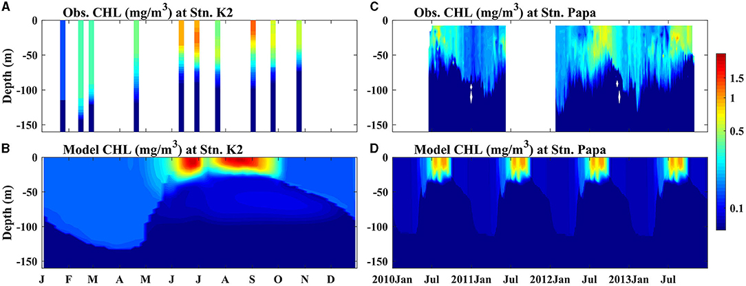
Figure 2. Seasonal cycle of chlorophyll concentrations (mg/m³) from (A,B) observation data and (C,D) the models for Stns. K2 and Papa. (A) Shows the observed values from every cruise observation from 2005 to 2013 at Stn. K2 and (B) shows the observed values from floats 6400 and 7601 during 2010–2013. The black dashed lines represent the MLD.

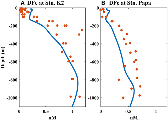
Figure 3. Comparison of the modeled distributions of the dissolved iron (DFe) concentration in the summer at (A) Stn. K2 and (B) Stn. Papa, with observations from Tagliabue et al. (2012), Schallenberg et al. (2015), and Nishioka et al. (2020). The blue solid line is the model result, and the solid circles are the observations.

Factors Affecting Phytoplankton Growth in the Western and Eastern Subarctic Pacific

The simulated seasonal cycle of bioavailable Fe, which was obtained by averaging the 5-year (2009–2013) model results, was compared with the small phytoplankton and diatom biomasses at Stn. K2 and Stn. Papa, respectively (Figure 4). The surface BFe at Stn. K2 and Stn. Papa both clearly increased with the deepening of the MLD before June, as the two phytoplankton biomasses remained almost stable at their minimum values. After mixed layer shoaling in May, the surface small phytoplankton and diatom biomasses began to increase in both regions, indicating the impacts of the MLD on the initialization of rapid growth in phytoplankton. Subsequently, at Stn. K2, the small phytoplankton reached their first peak (0.32 mmol N/m³) in mid-June, while the diatoms reached their maximum (1.46 mmol N/m³) later, at the end of June. When the surface BFe began to decrease in early July, the diatom biomass also decreased rapidly, but the small phytoplankton biomass gradually increased and reached its second peak (1.35 mmol N/m³) in mid-August. The high value of small phytoplankton biomass could last until the end of September, as the BFe decreased to a minimum of 0.19 nM. On the other hand, at Stn. Papa, where the surface BFe maximum was ~0.2 nM lower than at Stn. K2, the surface diatom biomass remained low (~0.1 mmol N/m³), although a slight increase occurred in summer. However, the peak of small phytoplankton biomass could reach up to 1.19 mmol N/m³ by the end of August; this value was close to the small phytoplankton biomass at Stn. K2. The magnitude of the modeled small phytoplankton biomass was consistent with that in a previous study, showing that the peak phytoplankton biomass in the eastern subarctic Pacific is similar to those in other subarctic regions, although the chlorophyll concentration does not reach the magnitude of seasonal phytoplankton blooms in other subarctic regions (Westberry et al., 2016). Therefore, the change in BFe plays a more important role in influencing diatom biomass than in influencing small phytoplankton biomass.

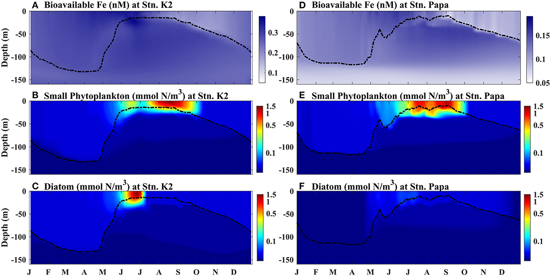
Figure 4. Modeled seasonal cycle of vertical profiles at (A–C) Stn. K2 and (D–F) Stn. Papa. (A,D) Bioavailable Fe (B,E), small phytoplankton biomass, and (C,F) diatom biomass. The black dashed lines represent the MLD.

Since the effect of bioavailable iron on phytoplankton dynamics was expressed in the model mainly as a limit on phytoplankton growth, the seasonal growth rates of small phytoplankton and diatoms in these two regions were provided (Figure 5). The growth rate of phytoplankton in this study was defined as the ratio of phytoplankton growth, which represents PP, to phytoplankton biomass. In winter, the surface growth rates of both types of phytoplankton reached their minimums, while the difference in the growth rates between the surface and the bottom of the mixed layer was much higher than that in summer. From winter to summer, the surface growth rates of phytoplankton began to increase, but the growth rates of diatoms were higher (lower) than those of small phytoplankton at Stn. K2 (Stn. Papa). This result suggests that the responses the phytoplankton growth in these two regions have to changes in the environment, e.g., light, differ between winter and summer. At the very least, this is because of the difference in the surface BFe between the western and eastern subarctic Pacific (Figures 4A,D).

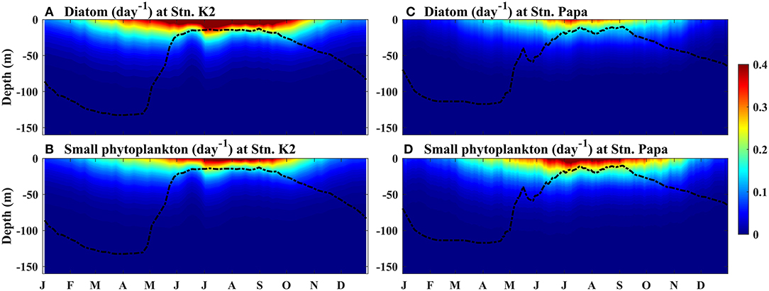
Figure 5. Modeled seasonal cycle of the growth rates of phytoplankton at (A,B) Stn. K2 and (C,D) Stn. Papa. (B,D) Small phytoplankton and, (A,C) diatoms. The black dashed lines represent the MLD.

To further investigate the factors controlling phytoplankton growth in these two regions, the vertically integrated growth rate, regulating factors, and limiting nutrient factors of phytoplankton were compared (Figures 6, 7). The growth rate of phytoplankton was determined by multiplying the maximum growth rate by the product of three regulating factors, i.e., nutrients, temperature, and light. Thus, for each regulated limiting factor, a higher value indicated a weaker limitation on phytoplankton growth. The regulation of limiting nutrients was identified on the basis of the minimum levels of the limiting nutrient factors, i.e., nitrate, phosphate, and BFe for small phytoplankton and nitrate, phosphate, BFe, and silicate for diatoms. Furthermore, the vertical integration method incorporated the influence of changes in the mixed layer on phytoplankton growth (a detailed description of the method is provided in section Model and Data).

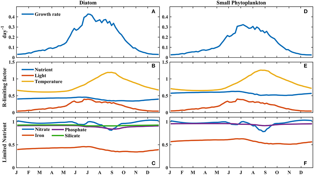
Figure 6. Modeled seasonal cycle of the vertically integrated (A,D) growth rate, (B,E) regulating factors, and (C,F) limiting nutrient factors for phytoplankton, weighted by the phytoplankton biomass at Stn. K2. (A–C) are for small phytoplankton; (D–F) are for diatoms.

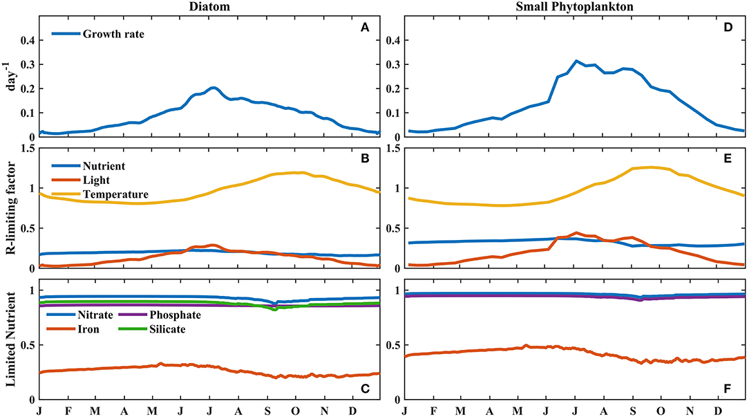
Figure 7. Modeled seasonal cycle of the vertically integrated (A,D) growth rate, (B,E) regulating factors, and (C,F) limiting nutrient factors for phytoplankton, weighted by the phytoplankton biomass at Stn. Papa. (A–C) are for small phytoplankton; (D–F) are for diatoms.

The time series of the growth rates of diatoms and small phytoplankton at Station K2 were characterized by a prominent seasonal cycle, with the highest values in July, i.e., ~0.42 and 0.31 day⁻¹, respectively (Figures 6A,D). In the winter, the growth rates of both phytoplankton were low, specifically at < 0.1 day⁻¹ between November and April. After May, the growth rates and regulating light factors both increased more rapidly, as the MLD became shallower. This result suggests that light limitation is the main factor controlling diatom and small phytoplankton growth in the winter, as deep mixing leads to low light availability within the mixed layer. In this study, since there was little difference between diatom biomass and small phytoplankton biomass in the winter (Figures 4B,C), the higher growth rates of the diatoms in the spring than that of small phytoplankton led to the diatom biomass being higher than the small phytoplankton biomass in the spring at Stn. K2. Transient decreases in growth rate and light were also observed for both phytoplankton types in early June. During this period, the high concentrations of diatoms at the surface prevented light from reaching the deep ocean, leading to a decrease in photosynthetically active radiation across the subsurface ocean. Correspondingly, the subsurface growth rates of small phytoplankton and diatoms at Stn. K2 both showed significant decreases (Figures 5A,B). Consequently, the decreases in the growth rates of small phytoplankton had a greater inhibitory effect on small plankton growth than microzooplankton grazing (Supplementary Figure 1) and resulted in a decrease in small phytoplankton biomass in mid-June. Diatoms, which have higher growth rates during this period, were less influenced by this transient decrease. As a result, diatom growth was still greater than diatom loss (Supplementary Figure 1), leading to an increase in diatom biomass until the end of June. With the intensified limitations on both light and nutrients in July, the diatom growth rate decreased rapidly and the diatom bloom terminated. Since the Fe limitation of the two phytoplankton types was persistently stronger than the limitations of the other limited nutrients (Figures 6C,F), the Fe limitation dominated the nutrient limitation on phytoplankton growth. However, the decrease in the growth rates of small phytoplankton was much smaller than that in the growth rates of diatoms in July, although the limitations of light and Fe on small phytoplankton also became stronger. Furthermore, the relatively small change in small phytoplankton growth from summer to autumn helped increase the low phytoplankton biomass until September, which was associated with a decline in microzooplankton grazing that was caused by the decrease in microzooplankton biomass (Supplementary Figures 1, 2). This result suggests that the differential changes in the growth rates of diatoms and small phytoplankton during summer play important roles in driving phytoplankton blooms in the western subarctic Pacific.

To further investigate the factors controlling the growth rates of diatoms and small phytoplankton in the western subarctic Pacific, the rates of decline in the two phytoplankton growth rates and the regulating limiting factors were investigated. During the summer, the phytoplankton bloom switched from diatom-dominated in early July to small phytoplankton-dominated in mid-August (Table 1). The decline in the growth rate of diatoms (14%) was more than two times that in the growth rate of small phytoplankton (5.7%). The strength of the Fe limitation of diatoms also decreased by 17%, which was more prominent than the decrease in its limitation of small phytoplankton (11%). In comparison, the other two regulating limiting factors on diatoms and small phytoplankton weakened to relatively similar degrees (<2% difference). This suggests that the decrease in BFe during the summer limits the growth of diatoms more strongly than it limits the growth of small phytoplankton.

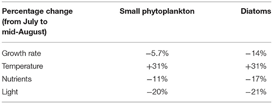
Table 1. Percent changes in the growth rates and the regulating factors of temperature, nutrients, and light from July to mid-August.

Similarly, at Stn. Papa, where the BFe in the upper ocean was lower than that at Stn. K2, the stronger Fe limitation caused the peak growth rate of diatoms to be just 0.2 day⁻¹, which was much lower than the peak growth rate of small phytoplankton (0.31 day⁻¹) (Figures 7A,D). When the Fe limitation gradually strengthened from summer to autumn, however, the relatively small change in small phytoplankton growth, which was associated with a decline in microzooplankton grazing caused by the decrease in microzooplankton biomass (Supplementary Figure 2), helped increase the small phytoplankton biomass until September, similar to the pattern observed at Stn. K2 (Figure 4E). To further illustrate the difference in the effect of BFe on phytoplankton growth between these two regions, the model was applied to evaluate the influences of different factors. In particular, the growth rate of phytoplankton was compared under the Fe limitation only and under the light and temperature limitation only at Stn. K2 and Stn. Papa (Figure 8). In each case, the value of light limitation and temperature was set to 1 or the value of nutrient limitation was set to 1. During the period from May to July, the difference in the average growth rate of the diatoms limited only by light and temperature between these two regions was 0.11 day⁻¹, which was much less than the difference in the average growth rate of the diatoms limited only by Fe (0.68 day⁻¹) (Figures 8A,B). This result suggests that the difference in Fe limitation contributes 86% of the higher diatom growth rate at Stn. K2 compared with Stn. Papa. However, the peak growth rate of small phytoplankton reached 0.94 day⁻¹ at Stn. K2 and 0.84 day⁻¹ at Stn. Papa; this was an ~11% decrease between Stn. K2 and Stn. Papa, while the peak growth rates of diatoms decreased by 45% between the two stations (Figures 8B,D). This result suggests that the influence of the difference in BFe between these two regions on small phytoplankton growth was much weaker than its influence on diatom growth.

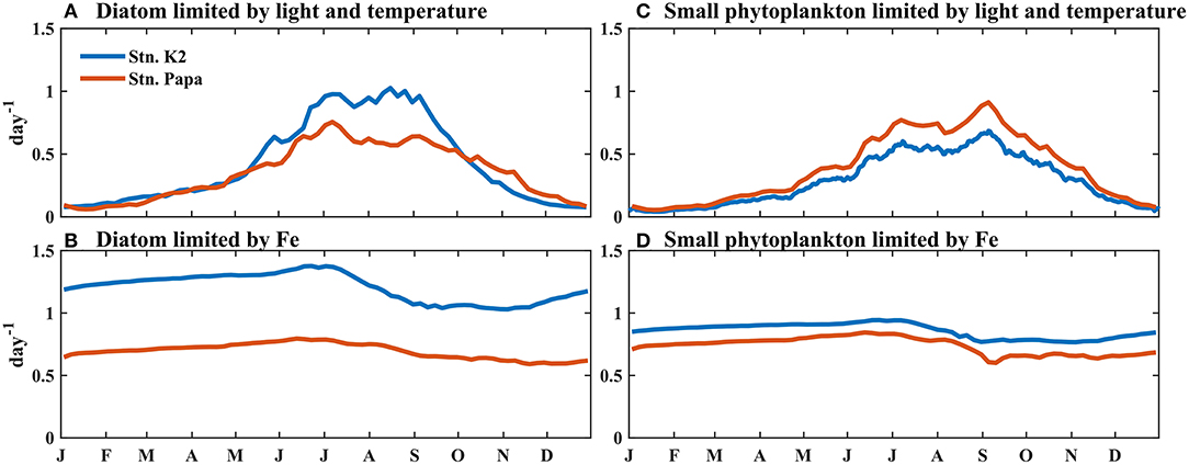
Figure 8. Modeled vertically integrated growth rate as limited by (A,C) light and temperature and (B,D) Fe for (A,B) diatoms and (C,D) small phytoplankton, weighted by the phytoplankton biomass. Note that the phytoplankton growth rate is limited only by (A,C) light and temperature, but Fe limitation is not considered; (B,D) are limited only by Fe, but temperature and light limitation are not considered.

Discussion

The Role of Fe in Phytoplankton Dynamics in the Western and Eastern Subarctic Pacific

The subarctic North Pacific is one of the three major high-nitrate, low-chlorophyll regions of the global ocean (Harrison et al., 2004). There is a major difference in marine systems between the western and eastern subarctic Pacific, i.e., the seasonality of phytoplankton blooms (Fujiki et al., 2009, 2014). In the western subarctic Pacific, two phytoplankton blooms have been observed from late spring to early summer and from late summer to autumn (Matsumoto et al., 2014). During the first bloom period, diatoms dominate the phytoplankton group, while small phytoplankton become the most abundant group during the second bloom period (Fujiki et al., 2014). In the eastern subarctic Pacific, there is only a single phytoplankton bloom from late summer to autumn, with small phytoplankton dominating the phytoplankton group; however, the chlorophyll concentration during this bloom does not reach the magnitude that the phytoplankton blooms in other high-latitude regions achieve (Westberry et al., 2016; Yang et al., 2018). Previous studies, by analyzing oceanographic data, have shown that the magnitude and durations of diatom blooms are controlled by Fe bioavailability (Fujiki et al., 2014; Shiozaki et al., 2014). The dissolved Fe concentration and the bioavailability of Fe are both higher in the western subarctic Pacific than in the eastern subarctic Pacific (Harrison et al., 2004; Nishioka et al., 2007; Kondo et al., 2021); these differences likely cause the observed differences in ecosystem dynamics, especially in diatom dynamics. Furthermore, to further investigate the role of Fe in the phytoplankton dynamics in these two regions, ecosystem models are required in order to realistically incorporate oceanic Fe cycling and Fe limitation on phytoplankton growth. Therefore, in this study, two 1D physical-biochemical coupled models with the Fe cycle, which included the conversion between different Fe species, were applied; one model was for Stn. K2, which is in the western subarctic Pacific, and the other was for Stn. Papa, which is in the eastern subarctic Pacific. The models successfully reproduced the physical and biogeochemical conditions observed by a cruise at Stn. K2 and by the BGC-Argo at Stn. Papa (Figures 1–3).

Since the vertical diffusivity in the upper ocean is sufficiently high to mix the water column well within the mixed layer, each individual phytoplankton cannot stay long enough at the surface where the light environment is suitable for growth (Kawamiya et al., 1995). As a result, when the MLD is deep enough, the growth of the mixed phytoplankton depends on the availability of light averaged within the mixed layer, which is much lower than that at the surface (Matsumoto et al., 2014). Thus, the seasonality of MLD reflects the variation in light availability to some extent. In the winter, the phytoplankton growth at the two stations was limited by low light availability caused by the deep MLD (Figures 6, 7); this finding was consistent with those of previous studies (Maldonado et al., 1999; Matsumoto et al., 2014). After mixed layer shoaling, the phytoplankton gradually acquired enough light, and Fe limitation began to control phytoplankton growth (Figures 6, 7). In contrast, a previous model without a Fe cycle used different parameter values to simulate the impact of Fe limitation on phytoplankton growth, and the model was applied to reproduce the ecological differences between the two mentioned regions (Fujii et al., 2007). The said study also indicated that the major ecological difference between the two was the weaker Fe limitation on phytoplankton growth in the western subarctic Pacific. The model in this study, which incorporated oceanic Fe cycling and Fe limitation withy phytoplankton growth, further validated the previous findings. Additionally, the results of this study showed that the growth rate of diatoms at Stn. K2 was nearly two times higher than that at Stn. Papa, with the differences in BFe between these two regions contributing ~86% of this difference (Figure 8). On the other hand, differences in BFe had less influence on the growth rate of small phytoplankton. As Fe was taken for phytoplankton growth, it gradually became deficient in the surface waters of the western Subarctic Pacific during the summer. Thus, by the end of summer, Fe became a major limiting factor for phytoplankton growth (Tsuda et al., 2003; Nishioka et al., 2011). The model results suggest that a decrease in BFe leads to stronger Fe limitation during the summer than earlier in the year, which subsequently induces a reduction in the growth rate of diatoms (Table 1). As a result, the diatom bloom terminates because of the decrease in BFe. On the other hand, the decrease in BFe during summer has little impact on small phytoplankton growth, and the corresponding high growth rate help maintain to increase of the small phytoplankton biomass until autumn. As a result, the lower BFe at Stn. Papa throughout the year limits diatom growth and prevents the occurrence of diatom blooms.

Since Fe limits phytoplankton growth in these two regions, particularly in the summer, a change in the Fe supply to the upper ocean, e.g., an increase in atmospheric dust, could affect biological production (Bishop et al., 2002; Hamme et al., 2010; Yoon et al., 2017). It is essential to understand Fe cycling processes and clarify the influences changes in Fe supply have on phytoplankton. Furthermore, the BFe in the mixed layer in the model is controlled by various processes (atmospheric dust deposition, BFe and inert Fe interconversion, phytoplankton uptake, and vertical diffusion). The seasonal variabilities of these processes within the mixed layer were compared in this study (Figure 9). In the winter, all the fluxes of the Fe processes were generally small in both regions. After MLD shoaling in the spring, atmospheric dust deposition and the conversion between BFe and inert Fe became the two largest sources of Fe in both regions. As a result, atmospheric dust deposition accounted for 60% of the total Fe at Stn. K2, but only contributed 23% at Stn. Papa. This result indicates that atmospheric dust deposition is more important in influencing the Fe cycle at Stn. K2 than at Stn. Papa. In line with this result, a previous study found that the flux of atmospherically deposited Fe in the western subarctic Pacific was much higher than that in the eastern subarctic Pacific (Mahowald et al., 2005). The conversion between BFe and inert Fe accounted for 33 and 69% of the total sources at Stn. K2 and at Stn. Papa, respectively. In the model, the conversion flux from inert Fe to BFe was related to photoreduction and the remineralization of plankton debris, which could increase BFe under higher phytoplankton-biomass conditions. As a result, the flux from inert Fe to BFe could increase under higher light and phytoplankton-biomass conditions (Lee and Fisher, 1993; Rijkenberg et al., 2005). The conversion flux from inert Fe to BFe is, therefore, highest during summer and replenishes the lost BFe that was absorbed by phytoplankton growth. After the MLD becomes deeper in late autumn, vertical diffusion becomes the largest source of Fe in the two regions, although all Fe fluxes decrease in size.

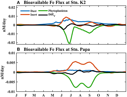
Figure 9. Modeled seasonal cycle of each source/sink term for bioavailable Fe averaged within the mixed layer due to phytoplankton uptake, vertical diffusion, dust, and the conversion between inert Fe and BFe at (A) Stn. K2 and (B) Stn. Papa.

Because the contributions of atmospheric deposition to BFe at Stn. K2 and Stn. Papa differ, a change in atmospheric Fe deposition would result in different phytoplankton responses in these two regions. In particular, a previous study showed that human activities would lead to more dissolved Fe and higher Fe bioavailability in the upper ocean (Krishnamurthy et al., 2009). However, the details of these dynamics remain largely unexplored. To further evaluate the influence of an increase in atmospheric Fe deposition on phytoplankton dynamics in the western and eastern subarctic Pacific, sensitivity experiments were carried out. Since the sources of dust for the western and eastern subarctic Pacific are considered to be the same (the Gobi Desert; Boyd et al., 1998), the increase in atmospheric Fe deposition due to human activities at Stn. K2 and Stn. Papa would presumably change with the same magnitude. The experiments were, therefore, forced with two (Exp 1), three (Exp 2), and four times (Exp 3) as much atmospherically deposited Fe as in the control runs at Stn. Papa and Stn. K2 after 2009. The vertical distributions of phytoplankton and zooplankton in the DFe Dep *2 experiment were examined from 2009 to 2011, which was when the atmospheric deposition of Fe increased (Figures 10, 11). In this study, the differences between the control run and the experimental case were analyzed by subtracting the daily output of the experimental case from that of the control run.

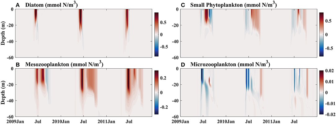
Figure 10. Modeled vertical distributions of differences in (A) diatoms (mmol N/m³), (B) small phytoplankton (mmol N/m³), (C) mesozooplankton (mmol N/m³), and (D) microzooplankton (mmol N/m³) between the control run and sensitivity experiment Exp 1, which was forced with two times the dissolved Fe dust deposition after 2009, at Stn. K2.

Figure 11. Modeled vertical distributions of differences in (A) diatoms (mmol N/m³), (B) small phytoplankton (mmol N/m³), (C) mesozooplankton (mmol N/m³), and (D) microzooplankton (mmol N/m³) between the control run and sensitivity experiment Exp 1, which was forced with two times the dissolved Fe dust deposition after 2009, at Stn. Papa.

In late spring and early summer, i.e., June to July, with the increase in atmospheric iron deposition, the diatom biomass in the upper ocean increased at both Stn. Papa and Stn. K2 (Figures 10A, 11A); however, the change was smaller at Stn. Papa than at Stn. K2. At Stn. Papa, the small increase in diatom biomass contributed little to the increase in mesozooplankton biomass, which consequently led to less grazing pressure on microzooplankton. In July, the low phytoplankton biomass also began to increase. Considering the increased food availability and lower grazing pressure due to the low abundance of mesozooplankton, microzooplankton populations rapidly increased (Figure 11D), which, in turn, limited the growth of small phytoplankton. In comparison, at Stn. K2, there were fewer microzooplankton starting in July, which was when the number of small phytoplankton increases (Figure 10D), thus inducing less grazing on small phytoplankton. As a result, the increase in small phytoplankton was smaller at Stn. Papa than at Stn. K2, although the atmospherically deposited Fe increased by the same amount in both regions. Indeed, the surface small phytoplankton biomass in 2009 increased by the maximum values of 0.85 mmol N m⁻³ at Stn. K2 and 0.42 mmol N m⁻³ at Stn. Papa, i.e., by ~63 and 35%, respectively (Figures 10C, 11C). However, the effects of the change in BFe on small phytoplankton growth in both regions were weak (Figures 6A, 7A). In late summer and autumn, i.e., August to September, the increasingly abundant small phytoplankton were grazed by microzooplankton at both Stn. Papa and Stn. K2; however, the additional microzooplankton were instantaneously consumed by mesozooplankton (Figures 10C,D, 11C,D). As a result, the biomasses of both mesozooplankton and small phytoplankton increased significantly, but the biomass of microzooplankton changed slightly. Consistent with previous in situ Fe fertilization experiments, the increase in atmospheric Fe deposition induced a more pronounced increase in mesozooplankton populations than in microzooplankton populations (Tsuda et al., 2009). A previous study has also indicated that the decrease in microzooplankton biomass reduces microzooplankton grazing on small phytoplankton during autumn in the subarctic Pacific (Matsumoto et al., 2014). Thus, as the small phytoplankton biomass continues to increase from August to September (Figure 10C), a small increase in the biomass of microzooplankton induces persistent low grazing pressure on small phytoplankton. The low grazing pressure then contributes to an increase in small phytoplankton at both Stn. K2 and Stn. Papa. Therefore, when atmospheric Fe deposition increases, the responses of top-down control on small phytoplankton by microzooplankton grazing and bottom-up control on diatoms are in good agreement with a previous study on phytoplankton dynamics in the subarctic Pacific (Harrison et al., 2004).

The roles of increased atmospherically deposited Fe in affecting PP in the different experiments were also evaluated at the two stations that were studied (Figure 12). During winter, the increase in PP in both was is small because the strong light limitation overwhelmed the influence of increasing atmospherically deposited Fe on phytoplankton growth. This result agreed well with the results of previous winter Fe-enrichment experiments, which showed no enhancement of phytoplankton growth (Boyd et al., 1995). In the first year with an increase in atmospherically deposited Fe (2009), the maximum PP at Stn. K2 increased from 990 mg C/m²/day in the control run to 1,238 mg C/m²/day in Exp 1, 1,352 mg C/m²/day in Exp 2, and 1,440 mg C/m²/day in Exp 3, which were ~25, 37, and 45% increases, respectively. During this period, the maximum PP increased from 590 to 731 mg C/m²/day in Exp 1, 871 mg C/m²/day in Exp 2, and 916 mg C/m²/day in Exp 3, which were ~24, 48, and 55% increases at Stn. Papa. The results suggest that the response of PP at Stn. Papa would be stronger than that at Stn. K2 in a scenario where there would be a gradual increase in atmospherically deposited Fe. In addition, because PP is thought to be able to constrain the number of fish and, in turn, an increase in PP could expand fisheries (Nielsen and Richardson, 1996; Chassot et al., 2010), similar absolute increases in PP (both ~400 mg C/m²/day) may cause the increase in dust Fe inputs to have an approximate influence on fisheries in the western and eastern subarctic Pacific. A previous modeling study showed that the current soluble Fe deposition amount could be two to five times higher than the preindustrial soluble Fe deposition amount in the North Pacific (Luo et al., 2008). Thus, the response of PP in the eastern subarctic Pacific could be stronger than that in the western subarctic Pacific in the future, considering the increase in atmospheric Fe deposition due to human activities. With the atmospheric deposition of Fe increasing from Exp 1 to Exp 3, the increase in PP became less prominent in both regions (Figures 12A,C). Macronutrients, such as nitrate, became deficient in the surface waters, and they replaced Fe to become the limiting factor for phytoplankton growth by the end of the summer (Figures 12B,D).

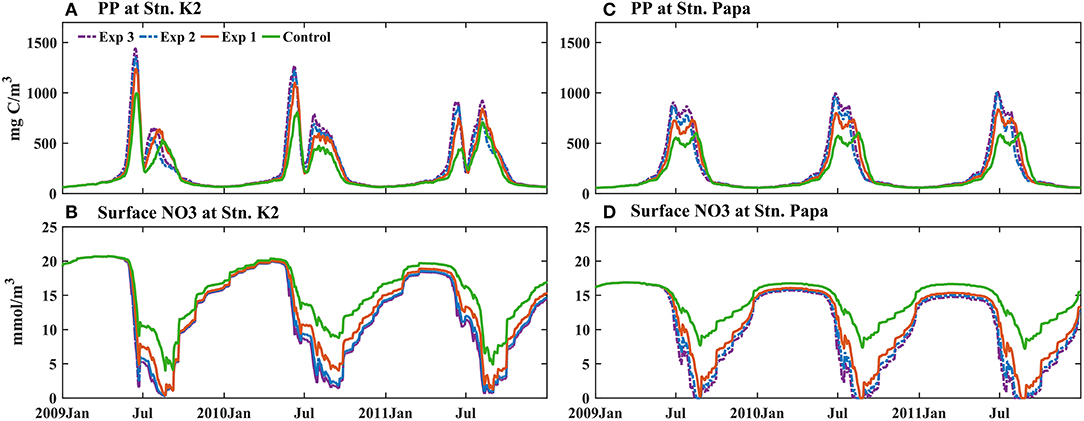
Figure 12. Modeled (A,C) primary production integrated over the upper 150 m (PP, mg C/m²/day) and (B,D) surface nitrate (SNO₃, mmol/m³) in different experiments forced by two (Exp 1), three (Exp 2), and four times (Exp 3) as much atmospherically deposited Fe as in the control run at (A,B) Stn. K2 and (C,D) Stn. Papa after 2009.

Assessing the Uncertainties in the Model

In this study, two one-dimensional physical-biological ocean models were used to simulate the marine ecosystems in the western and eastern subarctic Pacific. In these models, there were no horizontal advection or mesoscale processes, such as eddies, which are often important for transporting nutrients from the continental margin into the open ocean of the subarctic Pacific; e.g., previous studies have found that high concentrations of dissolved Fe in marginal seas, such as in the intermediate water of the Okhotsk Sea, would be transported long distances through the intermediate water layer to the open ocean of the western subarctic Pacific (Johnson et al., 2005; Lam et al., 2006; Nishioka et al., 2007, 2011; Yamashita et al., 2020; Misumi et al., 2021). However, Stn. K2 and Stn. Papa are both located far from the coast, where horizontal advection-induced coastal inputs, i.e., those from major rivers and coastal upwellings, have little influence on local biogeochemical processes. Therefore, a 1D model was appropriate for this study (Kawamiya et al., 1995; Denman and Pena, 1999; Sasai et al., 2016). Furthermore, mesoscale eddies in the subarctic Pacific are generally episodic and do not exhibit a prominent seasonal pattern, especially in the deep basin (Yasuda et al., 2000; Cummins and Lagerloef, 2004; Jackson et al., 2006). In addition, 1D models can better represent the mixed layer because they allow the vertical resolution to be increased; in contrast, 3D models are limited to coarse resolutions because of limitations on computational resources (Gan et al., 2006; Geng et al., 2019). However, without considering these 3D physical processes, the nutrient flux may be underestimated because of the effects of horizontal advection and mesoscale processes; e.g., the dissolved Fe concentration observed in the subsurface is higher than the modeled dissolved Fe concentration at the same depth (Figure 3). In this study, the seasonal variability in the vertical distribution of the chlorophyll concentration in the model was highly consistent with the observations, although the simulated chlorophyll concentration in the surface layer during winter and in the subsurface was slightly lower than the observation (Figure 2). This was, in part, because the phytoplankton increased the absorption of Fe to improve their photosynthetic capacity under low-irradiance conditions (Sunda and Huntsman, 1997). Because most of the Fe in the phytoplankton is involved in photosynthesis (Raven, 1988, 1990), a decrease in irradiance means an increase in the cellular Fe requirement of phytoplankton. This extracellular Fe allows synthesis of the photosynthetic units needed for low-light adaptation, which could also increase the growth rates of phytoplankton under low irradiance (Falkowski et al., 1981; Raven, 1990). However, this process was not incorporated into the model, resulting in slightly overestimated dissolved Fe concentrations and a lower chlorophyll concentration during winter in the subsurface (Figures 2, 3). In addition, few parameters were set to different values in the two models. Although the parameter differences between the two models would have led to a difference in the light limitations on phytoplankton between the two stations, the difference in Fe limitation dominated the difference in phytoplankton growth between the two stations (Figure 8). Therefore, using different parameters in the two models has little influence on the comparison of the roles of Fe in phytoplankton dynamics between the western and eastern subarctic Pacific.

Due to the influence of overwintering microzooplankton biomass on the small phytoplankton biomass in spring (Landry et al., 1993; Denman and Pena, 1999), sensitivity analyses of the grazing threshold for phytoplankton and microzooplankton were conducted (Supplementary Figure 3). These analyses found that the depth-integrated (0–150 m) chlorophyll concentration (IChl) with a higher grazing threshold for the small phytoplankton and diatoms was higher than that with a lower grazing threshold throughout the year, especially in the winter. In addition, the impact of the changes in the threshold for small phytoplankton on IChl exceeded that of the changes in the threshold for diatoms, which was consistent with the observation of the small phytoplankton dominating the community at Stn. Papa. Considering the model without the process where phytoplankton absorb more Fe to improve their photosynthetic capacity under low-irradiance conditions, the value of simulated IChl in winter, which is lower than the observed, would be within a reasonable range. When the grazing threshold value for microzooplankton becomes lower, however, the simulated IChl peak increases and the peak time of IChl is advanced. This result suggests that, when the overwintering microzooplankton biomass becomes higher, the grazing pressure of small phytoplankton becomes stronger, which further controls the small phytoplankton biomass in the spring.

Climatological seasonal deposition forcings that do not include episodic dust events were performed to drive the model, although the other forcings in the model were real-time data from the NCEP reanalysis I dataset from 2001 to 2014. Thus, the model could not reproduce the conditions in marine ecosystems during special atmospheric deposition events, e.g., the observed anomalous phytoplankton bloom due to volcanic ash fuels in 2008 (Hamme et al., 2010) and the anomalous increase in dissolved Fe in the depth range of 400–1,000 m due to the Siberian Forest fires at Stn. Papa (Schallenberg et al., 2017). In the latter case, the observations showed no enhancement of dissolved Fe concentrations or chlorophyll concentrations in response to the suspected deposition of aerosol (Schallenberg et al., 2017). Therefore, the model reproducing the seasonal patterns of chlorophyll concentration at Stn. Papa in 2012 is credible (Figure 2B). In the sensitivity experiments, the increased atmospheric deposition of Fe after 2009 was used to drive the model. When the additional Fe inputs in the model were increased, the dissolved Fe concentrations were projected to accumulate in the upper ocean. Therefore, the sensitivity experiments clearly showed that the dynamics of phytoplankton and zooplankton changed during the first year of increasing atmospheric Fe deposition, which was in 2009. Additionally, comparing the control run with the sensitivity experiments can help to evaluate the responses phytoplankton in both regions have to increases in atmospheric Fe deposition.

Conclusion

One major difference between the marine ecosystems of the western and eastern subarctic Pacific is the seasonal pattern of chlorophyll distribution. The underlying mechanism causing this difference is thought to be associated with Fe limitation. Thus, two 1D physical–biological models with Fe cycles were applied to evaluate the role of Fe in the phytoplankton dynamics of both regions and to investigate the phytoplankton responses to changes in atmospheric Fe deposition in the future. The model results showed that the lower level of BFe in the eastern subarctic Pacific resulted in a Fe limitation on diatom growth that was two times as strong as that in the western subarctic Pacific. The weaker Fe limitation in the western subarctic Pacific subsequently caused the diatom growth rate to be 86% higher than that in the eastern subarctic Pacific, with diatom blooms occurring in spring and early summer. However, the different concentrations of BFe had relatively weak effects on small phytoplankton, leading to similar growth rates for the small phytoplankton in both regions. Especially in the western subarctic Pacific, the Fe limitation became stronger during the summer, when BFe decreases, resulting in a decrease in the growth rate of diatoms. This leads to a rapid reduction in diatom biomass during summer and terminates the diatom bloom. In contrast, the observed decrease in BFe had little impact on small phytoplankton growth, which helped to maintain high levels of small phytoplankton biomass until autumn. Furthermore, the model sensitivity experiments suggested that the increase in atmospheric Fe deposition results in a significant increase in the biomasses of both diatoms and phytoplankton. In particular, the diatom population is bottom-up controlled, with additional BFe input leading to an increase in diatom growth. In contrast, the small phytoplankton population is mainly top-down controlled, with the decrease in microzooplankton grazing on small phytoplankton leading to an increase in small phytoplankton biomass. When the atmospheric deposition of Fe increases by the same rate in both regions, the increase in diatom biomass in the western subarctic Pacific, where the diatom biomass was higher than that in the eastern subarctic Pacific, leads to a more significant enhancement in the mesozooplankton biomass in spring and early summer. As a result, there is a higher grazing pressure on microzooplankton in the western subarctic Pacific during this period, leading to a smaller increase in microzooplankton biomass. Because of the lower grazing pressure on small phytoplankton from microzooplankton, the low phytoplankton biomass in the western subarctic Pacific increases more compared with that in the eastern subarctic Pacific in late summer. The increase in atmospheric Fe deposition also has a stronger influence on PP in the eastern subarctic Pacific than in the western subarctic Pacific; ~55 and 45% increases in PP occur, respectively, when the atmospheric Fe deposition increases by four times. However, the further elevation in the atmospheric deposition of Fe contributed less to the PP in both regions because the nutrient limitation on phytoplankton would change from a Fe limitation to a macronutrient limitation, such as a nitrate limitation. Therefore, this study contributes to a quantitative understanding of the role of Fe in the phytoplankton dynamics of the western and eastern subarctic Pacific and investigates the responses of marine ecosystems in the subarctic Pacific in future projected scenarios.

Data Availability Statement

The dataset used in this study includes the BGC-Argo float data (https://www.mbari.org/science/upper-ocean-systems/chemical-sensor-group/floatviz/), the cruise data in Western Subarctic North Pacific (http://www.godac.jamstec.go.jp/darwin/e.), the World Ocean Atlas (WOA18, https://www.ncei.noaa.gov/data/oceans/woa/WOA18/), the NCEP Reanalysis dataset (https://psl.noaa.gov/data/gridded/data.ncep.reanalysis.html), the global Fe dataset from GEOTRACES (https://www.bodc.ac.uk/geotraces/data/historical/) and Schallenberg et al. (2015) (http://dx.doi.org/10.1016/j.marchem.2015.04.004) and Nishioka et al. (2020) (https://eprints.lib.hokudai.ac.jp/dspace/handle/2115/77482.)

Author Contributions

H-RZ: investigation and writing. FC: conceptualization. PX: data curation. YQ and YW: review of the manuscript. All the authors have read and agreed to the published version of the manuscript.

Funding

This study was funded by the National Natural Science Foundation of China (41730536, 41890805).

Conflict of Interest

The authors declare that the research was conducted in the absence of any commercial or financial relationships that could be construed as a potential conflict of interest.

Publisher's Note

All claims expressed in this article are solely those of the authors and do not necessarily represent those of their affiliated organizations, or those of the publisher, the editors and the reviewers. Any product that may be evaluated in this article, or claim that may be made by its manufacturer, is not guaranteed or endorsed by the publisher.

Acknowledgments

We appreciate the dataset from the World Ocean Atlas (WOA18), the NCEP Reanalysis dataset, the float data, and the cruise data.

Supplementary Material

The Supplementary Material for this article can be found online at: https://www.frontiersin.org/articles/10.3389/fmars.2021.735826/full#supplementary-material

References

Banse, K., and English, D. C. (1999). Comparing phytoplankton seasonality in the eastern and western subarctic Pacific and the western Bering Sea. Prog. Oceanogr. 43, 235–288. doi: 10.1016/S0079-6611(99)00010-5
Behrenfeld, M. J., Hu, Y., O'Malley, R. T., Boss, E. S., Hostetler, C. A., Siegel, D. A., et al. (2017). Annual boom-bust cycles of polar phytoplankton biomass revealed by space-based lidar. Nat. Geosci. 10, 118–122. doi: 10.1038/ngeo2861
Bishop, J. K. B., Davis, R. E., and Sherman, J. T. (2002). Robotic observations of dust storm enhancement of carbon biomass in the North Pacific. Science 298, 817–821. doi: 10.1126/science.1074961
Bond, N. A., Cronin, M. F., Freeland, H., and Mantua, N. (2015). Causes and impacts of the 2014 warm anomaly in the NE Pacific. Geophys. Res. Lett. 42, 3414–3420. doi: 10.1002/2015GL063306
Boyd, P., and Harrison, P. J. (1999). Phytoplankton dynamics in the NE subarctic Pacific. Deep Sea Res. Part II Top. Stud. Oceanogr. 46, 2405–2432. doi: 10.1016/S0967-0645(99)00069-7
Boyd, P. W., Muggli, D. L., Varela, D. E., Goldblatt, R. H., Goldblatt, R., Orians, K. J., et al. (1996). In vitro iron enrichment experiments in the NE subarctic Pacific. Mar. Ecol. Prog. Ser. 136, 179–193. doi: 10.3354/meps136179
Boyd, P. W., Whitney, F. A., Harrison, P. J., and Wong, C. S. (1995). The NE subarctic Pacfic in winter: II. Biological rate processes. Mar. Ecol. Prog. Ser. 128, 25–34. doi: 10.3354/meps128025
Boyd, P. W., Wong, C. S., Merrill, J., Whitney, F., Snow, J., Harrison, P. J., et al. (1998). Atmospheric iron supply and enhanced vertical carbon flux in the NE subarctic Pacific: is there a connection? Global Biogeochem. Cycles 12, 429–441. doi: 10.1029/98GB00745
Chassot, E., Bonhommeau, S., Dulvy, N., Melin, F., Watson, R., Gascuel, D., et al. (2010). Global marine primary production constrains fisheries catches. Ecol. Lett. 13, 495–505. doi: 10.1111/j.1461-0248.2010.01443.x
Chien, C. T., Mackey, K. R. M., Dutkiewicz, S., Mahowald, N. M., Prospero, J. M., and Paytan, A. (2016). Effects of African dust deposition on phytoplankton in the western tropical Atlantic Ocean off Barbados. Global Biogeochem. Cycles 30, 716–734. doi: 10.1002/2015GB005334
Cummins, P. F., and Lagerloef, G. S. E. (2004). Wind-driven inter-annual variability over the northeast Pacific Ocean. Deep Sea Res. I Oceanogr. Res. Pap. 51, 2105–2121. doi: 10.1016/j.dsr.2004.08.004
de Boyer Montégut, C. (2004). Mixed layer depth over the global ocean: an examination of profile data 397 and a profile-based climatology. J. Geophys. Res. 109:C12003. doi: 10.1029/2004JC002378
Denman, K. L., and Pena, M. A. (1999). A coupled 1-D biological/physical model of the northeast subarctic Pacific Ocean with iron limitation. Deep Sea Res. Part II Top. Stud. Oceanogr. 46, 2877–2908. doi: 10.1016/S0967-0645(99)00087-9
Falkowski, P. G., Owens, T. G., Ley, A. C., and Mauzerall, D. C. (1981). Effects of growth irradiance levels on the ratio of reaction centers in two species of marine phytoplankton. Plant Physiol. 68, 969–973. doi: 10.1104/pp.68.4.969
Fasham, M. J. R. (2003). Ocean Biogeochemistry: The Role of the Ocean Carbon Cycle inGlobal Change, the IGBP Series. New York, NY: Springer.
Fennel, K., and Boss, E. (2003). Subsurface maxima of phytoplankton and chlorophyll: steady-state solutions from a simple model. Limnol. Oceanogr. 48, 1521–1534. doi: 10.4319/lo.2003.48.4.1521
Freeland, H. (2007). A short history of ocean station papa and line p. Prog. Oceanogr. 75, 120–125. doi: 10.1016/j.pocean.2007.08.005
Fujii, M., Yamanaka, Y., Nojiri, Y., Kishi, M. J., and Chai, F. (2007). Comparison of seasonal characteristics in biogeochemistry among the subarctic north Pacific stations described with a NEMURO-based marine ecosystem model. Ecol. Model. 202, 52–67. doi: 10.1016/j.ecolmodel.2006.02.046
Fujii, M., Yoshie, N., Yamanaka, Y., and Chai, F. (2005). Simulated biogeochemical responses to iron enrichments in three high nutrient, low chlorophyll (HNLC) regions. Prog. Oceanogr. 64, 307–324. doi: 10.1016/j.pocean.2005.02.017
Fujiki, T., Matsumoto, K., Honda, M. C., Kawakami, H., and Watanabe, S. (2009). Phytoplankton composition in the subarctic North Pacific during autumn 2005. J. Plankton Res. 31, 179–191. doi: 10.1093/plankt/fbn108
Fujiki, T., Matsumoto, K., Mino, Y., Sasaoka, K., Wakita, M., Kawakami, H., et al. (2014). The seasonal cycle of phytoplankton community structure and photo-physiological state in the western subarctic gyre of the North Pacific. Limnol. Oceanogr. 59, 887–900. doi: 10.4319/lo.2014.59.3.0887
Gan, J. P., Li, H., Curchitser, E. N., and Haidvogel, D. B. (2006). Modeling South China Sea circulation: response to seasonal forcing regimes. J. Geophys. Res. 111:C06034. doi: 10.1029/2005JC003298
Garcia, H. E., Weathers, K., Paver, C. R., Smolyar, I., Boyer, T. P., Locarnini, R. A., et al. (2018). “World Ocean Atlas 2018,” Vol. 4. Dissolved Inorganic Nutrients (phosphate, nitrate and nitrate+nitrite, silicate). A. Mishonov Technical Ed. NOAA Atlas NESDIS 84, 35p.
Geng, B., Xiu, P., Shu, C., Zhang, W. Z., Chai, F., Li, S., et al. (2019). Evaluating the roles of wind and buoyancy flux induced mixing on phytoplankton dynamics in the northern and central South China Sea. J. Geophys. Res. Ocean. 124, 680–702. doi: 10.1029/2018JC014170
Gledhill, M., and Buck, K. N. (2012). The organic complexation of iron in the marine environment: A review. Front. Microbiol. 3:69. doi: 10.3389/fmicb.2012.00069
Hamme, R. C., Webley, P. W., Crawford, W. R., Whitney, F. A., DeGrandpre, M. D., Emerson, S. R., et al. (2010). Volcanic ash fuels anomalous plankton bloom in subarctic northeast Pacific. Geophys. Res. Lett. 37:L19604. doi: 10.1029/2010GL044629
Harrison, P. J. (2002). Station Papa time series: insights into ecosystem dynamics. J. Oceanogr. 58, 259–264. doi: 10.1023/A:1015857624562
Harrison, P. J., Boyda, P. W., Varela, D. E., Takeda, S., Shiomoto, A., and Odate, T. (1999). Comparison of factors controlling phytoplankton productivity in the NE and NW subarctic Pacific gyres. Prog. Oceanogr. 43, 205–234. doi: 10.1016/S0079-6611(99)00015-4
Harrison, P. J., Whitney, F. A., Tsuda, A., Saixop, H., and Tadokoro, K. (2004). Nutrient and Plankton dynamics in the NE and NW gyres of the subarctic pacific ocean. J. Oceanogr. 60, 93–117. doi: 10.1023/B:JOCE.0000038321.57391.2a
Haskell, W. Z., Fassbender, A. J., Long, J. S., and Plant, J. N. (2020). Annual net community production of particulate and dissolved organic carbon from a decade of biogeochemical profiling float observations in the northeast pacific. Global Biogeochem. Cycles 34:e2020GB006599. doi: 10.1029/2020GB006599
Honda, M. C., and Watanabe, S. (2007). Utility of an automatic water sampler to observe seasonal variability in nutrients and DIC in the Northwestern North Pacific. J. Oceanogr. 63:349362. doi: 10.1007/s10872-007-0034-5
Huston, M. A., and Wolverton, S. (2009). The global distribution of net primary production: resolving the paradox. Ecol. Monogr. 79, 343–377. doi: 10.1890/08-0588.1
Imai, K., Nojiri, Y., Tsurushima, N., and Saino, T. (2002). Time series of seasonal variation of primary productivity at station KNOT (44° N, 155° E) in the sub-arctic western North Pacific. Deep Sea Res. Part II Top. Stud. Oceanogr. 49, 5395–5408. doi: 10.1016/S0967-0645(02)00198-4
Ito, A., and Shi, Z. (2016). Delivery of anthropogenic bioavailable iron from mineral dust and combustion aerosols to the ocean. Atmos. Chem. Phys. 16, 85–99. doi: 10.5194/acp-16-85-2016
Jackson, J. M., Myers, P. G., and Ianson, D. (2006). An examination of advection in the northeast Pacific Ocean, 2001-2005. Geophys. Res. Lett. 33:L15601. doi: 10.1029/2006GL026278
Jiang, M., Barbeau, K. A., Selph, K. E., Measures, C. I., Buck, K. N., Azam, F., et al. (2013). The role of organic ligands in iron cycling and primary productivity in the Antarctic Peninsula: a modeling study. Deep Sea Res. Part II Top. Stud. Oceanogr. 90, 112–133. doi: 10.1016/j.dsr2.2013.01.029
Jickells, T. D., An, Z. S., Andersen, K. K., Baker, A. R., Bergametti, G., Brooks, N., et al. (2005). Global iron connections between desert dust, ocean biogeochemistry, and climate. Science 308, 67–71. doi: 10.1126/science.1105959
Johnson, W. K., Miller, L. A., Sutherland, N. E., and Wong, C. S. (2005). Iron transport by mesoscale Haida eddies in the Gulf of Alaska. Deep Sea Res. Part II Top. Stud. Oceanogr. 52, 933–953. doi: 10.1016/j.dsr2.2004.08.017
Kalnay, E., Kanamitsu, M., Kistler, R., Collins, W., Deaven, D., Gandin, L., et al. (1996). The NCEP/NCAR 40-year reanalysis project. B. Am. Meteorol. Soc. 77, 437–472. doi: 10.1175/1520-0477(1996)077<0437:TNYRP>2.0.CO;2
Kawamiya, M., Kishi, M. J., Yamanaka, Y., and Suginohara, N. (1995). An ecological-physical coupled model applied to station papa. J. Oceanogr. 51, 635–664. doi: 10.1007/BF02235457
Kishi, M. J., Motono, H., Kashiwai, M., and Tsuda, A. (2001). An ecological-physical coupled model with ontogenetic vertical migration of zooplankton in the northwestern Pacific. J. Oceanogr. 57, 499–507. doi: 10.1023/A:1021517129545
Kobari, K., and Ikeda, T. (1999). Vertical distribution, population structure and life cycle of Neocalanuscristatus (Crustacea: Copepoda) in the Oyashio region, with notes on its regional variations. Mar. Biol. 134, 683–696. doi: 10.1007/s002270050584
Kondo, Y., Bamba, R., Obata, H., Nishioka, J., and Takeda, S. (2021). Distinct profiles of size-fractionated iron-binding ligands between the eastern and western subarctic Pacific. Sci. Rep. 11:2053. doi: 10.1038/s41598-021-81536-6
Krishnamurthy, A., Moore, J. K., Mahowald, N., Luo, C., Doney, S. C., Lindsay, K., et al. (2009). Impacts of increasing anthropogenic soluble iron and nitrogen deposition on ocean biogeochemistry. Global Biogeochem. Cycles 23:GB3016. doi: 10.1029/2008GB003440
Krishnamurthy, A., Moore, J. K., Mahowald, N., Luo, C., and Zender, C. S. (2010). Impacts of atmospheric nutrient inputs on marine biogeochemistry. J. Geophys. Res. 115:G01006. doi: 10.1029/2009JG001115
Lam, P. J., Bishop, J. K. B., Henning, C. C., Marcus, M. A., Waychunas, G. A., and Fung, I. Y. (2006). Wintertime phytoplankton bloom in the subarctic Pacific supported by continental margin iron. Global Biogeochem. Cycles 20:GB1006. doi: 10.1029/2005GB002557
Lamborg, C. H., Buesseler, K. O., and Lam, P. J. (2008). Sinking fluxes of minor and trace elements in the north Pacific Ocean measured during the vertigo program. Deep Sea Res. Part II Top. Stud. Oceanogr. 55, 1564–1577. doi: 10.1016/j.dsr2.2008.04.012
Landry, M. R., Monger, B. C., and Selph, K. E. (1993). Time-dependency of microzooplankton grazing and phytoplankton growth in the subarctic Pacific. Prog. Oceanogr. 32, 205–222. doi: 10.1016/0079-6611(93)90014-5
Large, W. G., McWilliams, J. C., and Doney, S. C. (1994). Oceanic vertical mixing: a review and a model with a nonlocal boundary layer parameterization. Rev. Geophys. 32:363. doi: 10.1029/94RG01872
Lee, B. G., and Fisher, N. S. (1993). Release rates of trace elements and protein from decomposing planktonic debris. 1. phytoplankton debris. J. Mar. Res. 51, 391–421. doi: 10.1357/0022240933223774
Luo, C., Mahowald, N., Bond, T., Chuang, P. Y., Artaxo, P., Siefert, et al. (2008). Combustion iron distribution and deposition. Global Biogeochem. Cycles 22:GB1012. doi: 10.1029/2007GB002964
Ma, W., Xiu, P., Chai, F., and Li, H. (2019). Seasonal variability of the carbon export in the central South China Sea. Ocean Dyn. 69, 955–966. doi: 10.1007/s10236-019-01286-y
Mackas, D. L., and Tsuda, A. (1999). Mesozooplankton in the eastern and western subarctic Pacific: community structure, seasonal life histories, and interannual variability. Prog. Oceanogr. 43, 335–363. doi: 10.1016/S0079-6611(99)00012-9
Mahowald, N. M., Baker, A. R., Bergametti, G., Brooks, N., Duce, A., Jickells, T. D., et al. (2005). Atmosphericglobal dust cycle and iron inputs to the ocean. Global Biogeochem. Cycles 19:GB4025. doi: 10.1029/2004GB002402
Mahowald, N. M., Engelstaedter, S., Luo, C., Sealy, A., Artaxo, P., Benitez-Nelson, C., et al. (2009). Atmospheric iron deposition: global distribution, variability, and human perturbations. Annu. Rev. Mar. Sci. 1, 245–278. doi: 10.1146/annurev.marine.010908.163727
Maldonado, M. T., Boyd, P. W., Harrison, P. J., and Price, N. M. (1999). Co-limitation of phytoplankton growth by light and Fe during winter in the NE subarctic Pacific Ocean. Deep Sea Res. Part II Top. Stud. Oceanogr. 46, 2475–2485. doi: 10.1016/S0967-0645(99)00072-7
Marchetti, A., Juneau, P., Whitney, F. A., Wong, C. S., and Harrison, P. J. (2006a). Phytoplankton processes during a mesoscale iron enrichment in the NE subarctic Pacific: Part II – Nutrient utilization. Deep Sea Res. Part II Top. Stud. Oceanogr. 53, 2114–2130. doi: 10.1016/j.dsr2.2006.05.031
Marchetti, A., Sherry, N. D., Kiyosawa, H., Tsuda, A., and Harrison, P. J. (2006b). Phytoplankton processes during a mesoscale iron enrichment in the NE subarctic Pacific: Part I—Biomass and assemblage. Deep Sea Res. Part II Top. Stud. Oceanogr. 53, 2095–2113. doi: 10.1016/j.dsr2.2006.05.038
Martin, J. H., and Fitzwater, S. E. (1988). Iron deficiency limits phytoplankton growth in the north-east Pacific subarctic. Nature 331, 341–343. doi: 10.1038/331341a0
Martin, J. H., Fitzwater, S. E., and Gordon, R. M. (1991). We still say iron deficiency limits phytoplankton growth in the subarctic Pacific. J. Geophys. Res. 96, 20699–20700. doi: 10.1029/91JC01935
Matsumoto, K., Honda, M. C., Sasaoka, K., Wakita, M., Kawakami, H., and Watanabe, S. (2014). Seasonal variability of primary production and phytoplankton biomass in the western Pacific subarctic gyre: control by light availability within the mixed layer. J. Geophys. Res. Oceans 119, 6523–6534. doi: 10.1002/2014JC009982
Miller, C. B., Frost, B. W., Wheeler, P. A., Landry, M. R., Welschmeyer, N., and Powell, T. M. (1991). Ecological dynamics in the sub-arctic Pacific, a possibly iron-limited ecosystem. Limnol. Oceanogr. 36, 1600–1615. doi: 10.4319/lo.1991.36.8.1600
Misumi, K., Nishioka, J., Obata, H., Tsumune, D., Tsubono, T., Long, M. C., et al. (2021). Slowly sinking particles underlie dissolved iron transport across the Pacific Ocean. Glob. Biogeochem. Cycle 35:e2020GB006823. doi: 10.1029/2020GB006823
Mochizuki, M., Shiga, N., Saito, M., Imai, K., and Nojiri, Y. (2002). Seasonal changes in nutrients, chlorophyll a and the phytoplankton assemblage of the western subarctic gyre in the Pacific Ocean. Deep Sea Res. Part II Top. Stud. Oceanogr. 49, 5421–5439. doi: 10.1016/S0967-0645(02)00209-6
Moore, J. K., Doney, S. C., and Lindsay, K. (2004). Upper ocean ecosystem dynamics and iron cycling in a global three-dimensional model. Global Biogeochem. Cycles 18:GB4028. doi: 10.1029/2004GB002220
Nielsen, E., and Richardson, K. (1996). Can changes in the fisheries yield in the Kattegat (1950–1992) be linked to changes in primary production? ICES J. Mar. Sc. 53, 988–994. doi: 10.1006/jmsc.1996.0123
Nishioka, J., and Obata, H. (2017). Dissolved iron distribution in the western and central subarctic Pacific: HNLC water formation and biogeochemical processes. Limnol. Oceanogr. 62, 2004–2022. doi: 10.1002/lno.10548
Nishioka, J., Obata, H., Hirawake, T., Kondo, Y., Yamashita, Y., Misumi, K., et al. (2021). A review: iron and nutrient supply in the subarctic Pacific and its impact on phytoplankton production. J. Oceanogr. 77, 561–587. doi: 10.1007/s10872-021-00606-5
Nishioka, J., Obata, H., Ogawa, H., Ono, K., Yamashita, Y., Lee, K., et al. (2020). Subpolar marginal seas fuel the North Pacific through the intermediate water at the termination of the global ocean circulation. Proc. Natl. Acad. Sci. U. S. A. 117, 12665–12673. doi: 10.1073/pnas.2000658117
Nishioka, J., Ono, T., Saito, H., Nakatsuka, T., Takeda, S., Yoshimura, T., et al. (2007). Iron supply to the western subarctic Pacific: importance of iron export from the Sea of Okhotsk. J. Geophys. Res. 112:C10012. doi: 10.1029/2006JC004055
Nishioka, J., Ono, T., Saito, H., Sakaoka, K., and Yoshimura, T. (2011). Oceanic iron supply mechanisms which support the spring diatom bloom in the Oyashio region, western subarctic Pacific. J. Geophys. Res. Oceans 116:C02021. doi: 10.1029/2010JC006321
Nishioka, J., Takeda, S., Kudo, I., Tsumune, D., Yoshimura, T., Kuma, K., et al. (2003). Size-fractionated iron distribution and iron-limiting processes in the subarctic NW Pacific. Geophys. Res. Lett. 30:1730. doi: 10.1029/2002GL016853
Obayashi, Y., Tanoue, E., Suzuki, K., Handa, N., Nojiri, Y., and Wong, C. S. (2001). Spatial and temporal variabilities of phytoplankton community structure in the northern North Pacific as determined by phytoplankton pigments. Deep Sea Res. Part I Oceanogr. Res. Pap. 48, 439–469. doi: 10.1016/S0967-0637(00)00036-4
Pena, M. A. (2003). Modelling the response of the planktonic food web to iron fertilization and warming in the NE subarctic Pacific. Prog. Oceanogr. 57, 453–479. doi: 10.1016/S0079-6611(03)00110-1
Pena, M. A., and Varela, D. E. (2007). Seasonal and interannual variability in phytoplankton and nutrient dynamics along line P in the NE subarctic Pacific. Prog. Oceanogr. 75, 200–222. doi: 10.1016/j.pocean.2007.08.009
Plant, J. N., Johnson, K. S., Sakamoto, C. M., Jannasch, H. W., Coletti, L. J., Riser, S. C., et al. (2016). Net community production at Ocean Station Papa observed with nitrate and oxygen sensors on profiling floats. Global Biogeochem. Cycles 30, 859–879. doi: 10.1002/2015GB005349
Raven, J. A. (1988). The iron and molybdenum use efficiencies of plant growth with different energy, carbon and nitrogen sources. New Phytol. 109, 279–287.
Raven, J. A. (1990). Predictions of Mn and Fe use efficiencies of phototrophic growth as a function of light availability for growth and C assimilation pathway. New Phytol. 116, 1–18. doi: 10.2307/2560409
Rijkenberg, M., Fischer, A. C., Kroon, J. J., Gerringa, L., Timmermans, K. R., Wolterbeek, H. T., et al. (2005). The influence of UV irradiation on the photoreduction of iron in the Southern Ocean. Mar. Chem. 93, 119–129. doi: 10.1016/j.marchem.2004.03.021
Sasai, Y., Yoshikawa, C., Smith, S. L., Hashioka, T., Matsumoto, K., Wakita, M., et al. (2016). Coupled 1-D physical-biological model study of phytoplankton production at two contrasting time-series stations in the western North Pacific. J. Oceanogr. 72, 509–526. doi: 10.1007/s10872-015-0341-1
Schallenberg, C., Davidson, A. B., Simpson, K. G., Miller, L. A., and Cullen, J. T. (2015). Iron(II) variability in the northeast subarctic Pacific Ocean. Mar. Chem. 177, 33–44. doi: 10.1016/j.marchem.2015.04.004
Schallenberg, C., Ross, A. R. S., Davidson, A. B., Stewart, G. M., and Cullen, J. T. (2017). Temporal variability of dissolved iron species in the mesopelagic zone at Ocean Station PAPA. J. Marine Sys. 172, 128–136. doi: 10.1016/j.jmarsys.2017.03.006
Shigemitsu, M., Okunishi, T., Nishioka, J., Sumata, H., Hashioka, T., Aita, M. N., et al. (2012). Development of a one-dimensional ecosystem model including the iron cycle applied to the Oyashio region, western subarctic Pacific. J. Geophys. Res. Oceans 117:C06021. doi: 10.1029/2011JC007689
Shiozaki, T., Ito, S., Takahashi, K., Saito, H., Nagata, T., and Furuya, K. (2014). Regional variability of factors controlling the onset timing and magnitude of spring algal blooms in the northwestern North Pacifc. J. Geophys. Res. Oceans 119, 1–13. doi: 10.1002/2013JC009187
Simon, N., Cras, A. L., Foulon, E., and Lemée, R. (2009). Diversity and evolution of marine phytoplankton. C. R. Biol. 332, 159–170. doi: 10.1016/j.crvi.2008.09.009
Sunda, W. G., and Huntsman, S. A. (1997). Interrelated influence of iron, light and cell size on marine phytoplankton growth. Nature 390, 389–392. doi: 10.1038/37093
Tagliabue, A., Mtshali, T., Aumont, O., Bowie, A. R., Klunder, M. B., Roychoudhury, A. N., et al. (2012). A global compilation of dissolved iron measurements: focus on distributions and processes in the Southern Ocean. Biogeosciences 9, 2333–2349. doi: 10.5194/bg-9-2333-2012
Tagliabue, T., Aumont, O., and Bopp, L. (2014). The impact of different external sources of iron in the global carbon cycle. Geophys. Res. Lett. 41, 920–926. doi: 10.1002/2013GL059059
Timothy, D. A., Wong, C. S., Barwell-Clarke, J. E., Page, J. S., White, L. A., and Macdonald, R. W. (2013). Climatology of sediment flux and composition in the subarctic northeast Pacific Ocean with biogeochemical implications. Prog. Oceanogr. 116, 95–129. doi: 10.1016/j.pocean.2013.06.017
Tsuda, A., Saito, H., Machida, R. J., and Shimode, S. (2009). Meso- and microzooplankton responses to an in-situ iron fertilization experiment (seeds ii) in the northwest subarctic Pacific. Deep Sea Res. Part II Top. Stud. Oceanogr. 56, 2767–2778. doi: 10.1016/j.dsr2.2009.06.004
Tsuda, A., Takeda, S., Saito, H., Nishioka, J., Nojiri, Y., Kudo, I., et al. (2003). A mesoscale iron enrichment in the western subarctic Pacific induces a large centric diatom bloom. Science 300, 958–961. doi: 10.1126/science.1082000
Westberry, T. K., Schultz, P., Behrenfeld, M. J., Dunne, J. P., Hiscock, M. R., Maritorena, S., et al. (2016). Annual cycles of phytoplankton biomass in the subarctic Atlantic and Pacific Ocean. Global Biogeochem. Cycles 30, 175–190. doi: 10.1002/2015GB005276
Xiu, P., and Chai, F. (2021). Impact of atmospheric deposition on carbon export to the deep ocean in the subtropical Northwest Pacific. Geophys. Res. Lett. 48:e2020GL089640. doi: 10.1029/2020GL089640
Yamashita, Y., Nishioka, J., Obata, H., and Ogawa, H. (2020). Shelf humic substances as carriers for basin-scale iron transport in the North pacific. Sci. Rep. 10:4505. doi: 10.1038/s41598-020-61375-7
Yang, B., Emerson, S. R., and Peña, M. A. (2018). The effect of the 2013–2016 high temperature anomaly in the subarctic Northeast Pacific (the “Blob”) on net community production. Biogeosciences 15, 6747–6759. doi: 10.5194/bg-15-6747-2018
Yasuda, I., Ito, S. I., Shimizu, Y., Ichikawa, K., and Koizumi, K. (2000). Cold-core anticyclonic eddies south of the bussol' strait in the northwestern subarctic Pacific. J. Phys. Oceanogr. 30, 1137–1157. doi: 10.1175/1520-0485(2000)030<1137:CCAESO>2.0.CO;2
Keywords: subarctic north Pacific, iron limitation, phytoplankton dynamics, seasonal variation, future change
Citation: Zhang H-R, Wang Y, Xiu P, Qi Y and Chai F (2021) Roles of Iron Limitation in Phytoplankton Dynamics in the Western and Eastern Subarctic Pacific. Front. Mar. Sci. 8:735826. doi: 10.3389/fmars.2021.735826
Received: 03 July 2021; Accepted: 16 August 2021;
Published: 17 September 2021.
Edited by:
Jian Ma, Xiamen University, ChinaReviewed by:
Tom Trull, Commonwealth Scientific and Industrial Research Organisation (CSIRO), AustraliaRuifeng Zhang, Shanghai Jiao Tong University, China
Copyright © 2021 Zhang, Wang, Xiu, Qi and Chai. This is an open-access article distributed under the terms of the Creative Commons Attribution License (CC BY). The use, distribution or reproduction in other forums is permitted, provided the original author(s) and the copyright owner(s) are credited and that the original publication in this journal is cited, in accordance with accepted academic practice. No use, distribution or reproduction is permitted which does not comply with these terms.
*Correspondence: Yuntao Wang, yuntao.wang@sio.org.cn