
Applications of TLS and ALS in Evaluating Forest Ecosystem Services: A Southern Carpathians Case Study

 , ,
, ,
Abstract
:1. Introduction
2. Materials and Methods
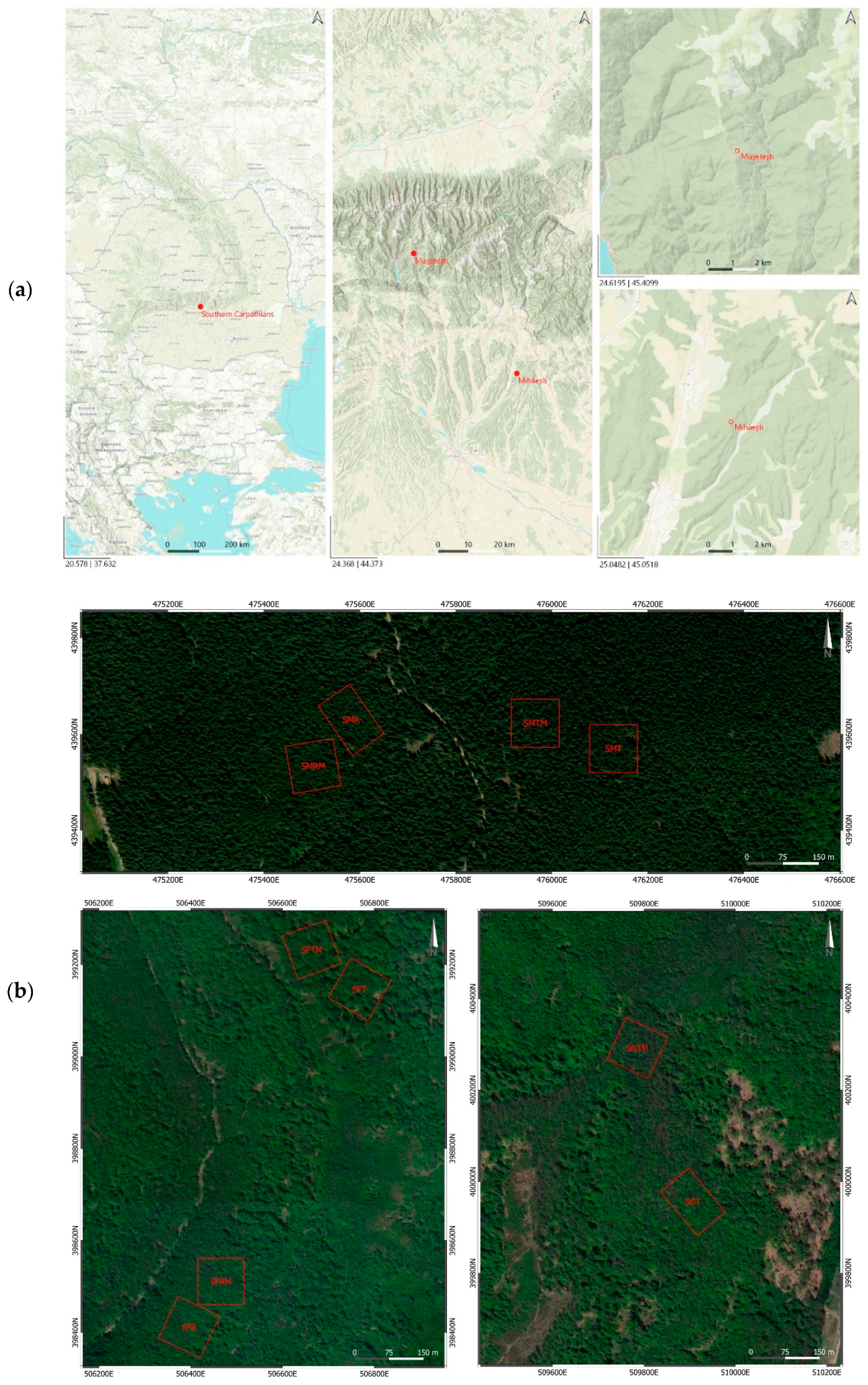
2.1. Study Site
2.2. Conventional Field Data Collection
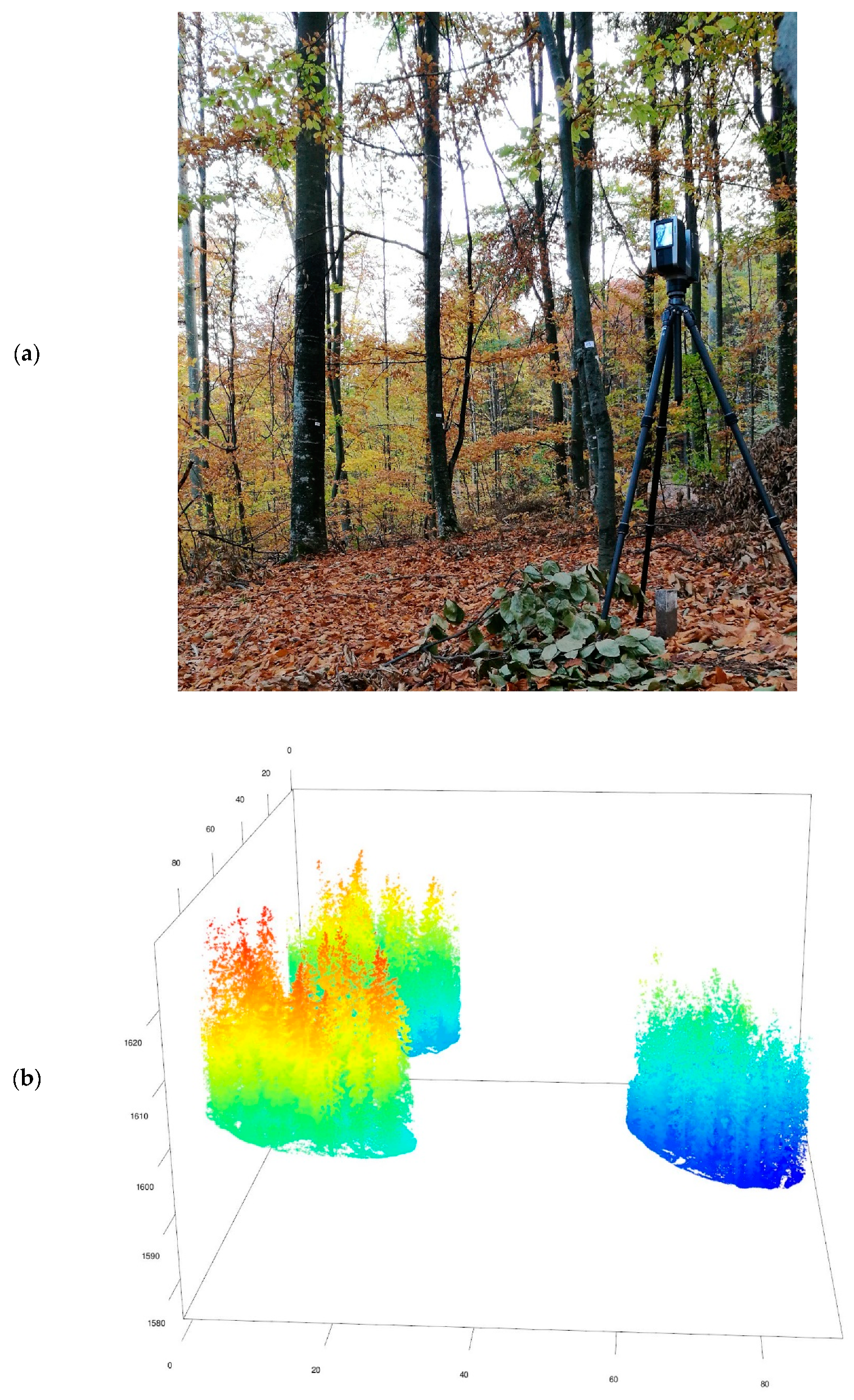
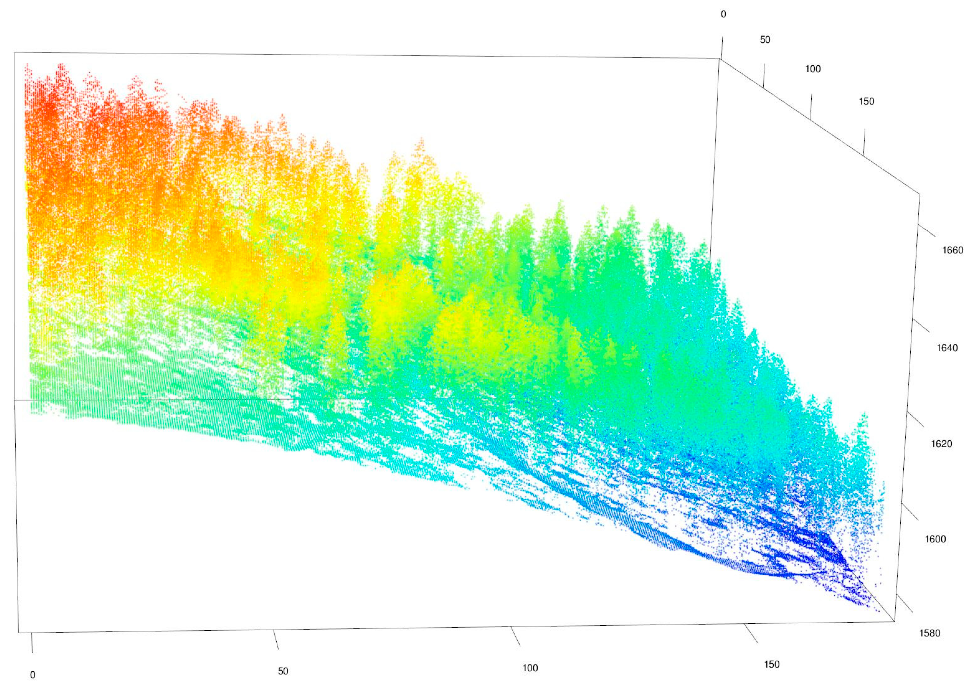
2.3. Terrestrial Laser Scanner Data
2.4. Airborne Laser Scanner Data
2.5. Ecosystem Services Identification and Evaluation
3. Results
3.1. Provisioning Services
3.2. Regulating Services
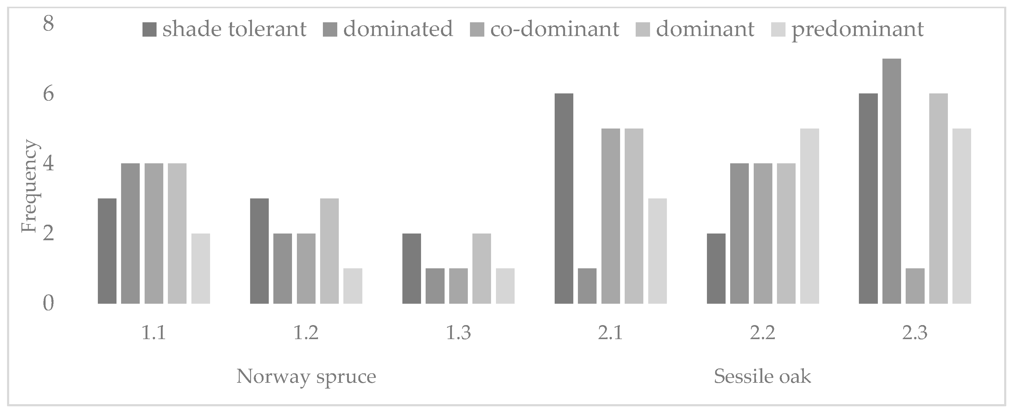
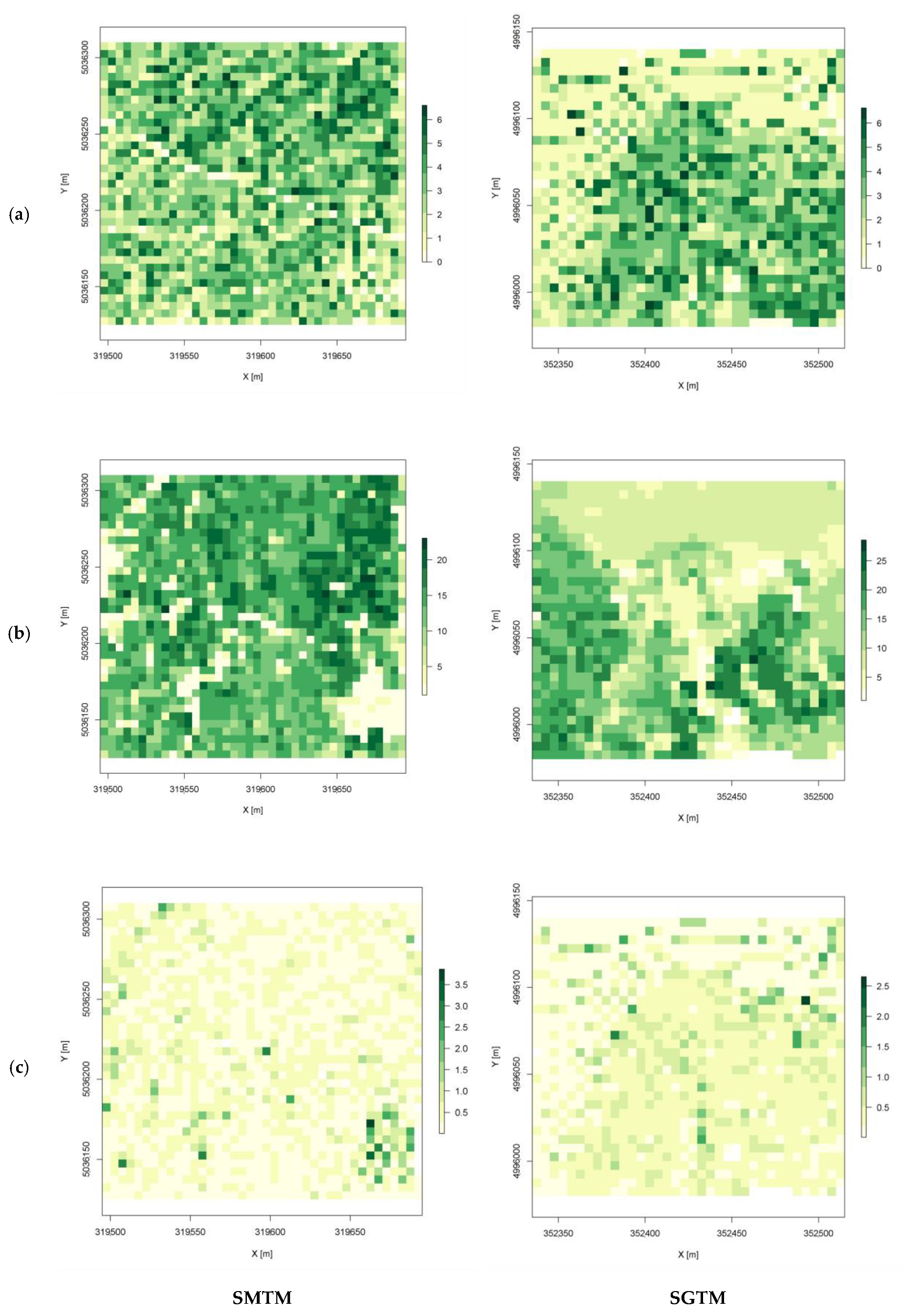
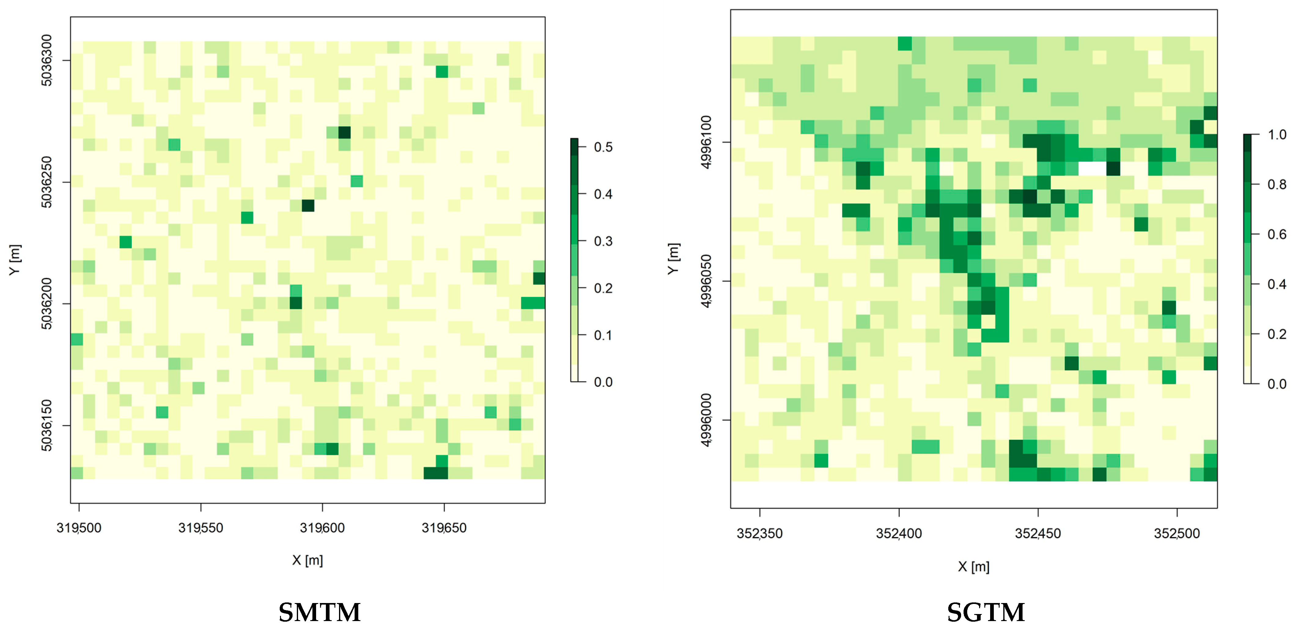
3.2.1. Structural Indices
3.2.2. Carbon Storage
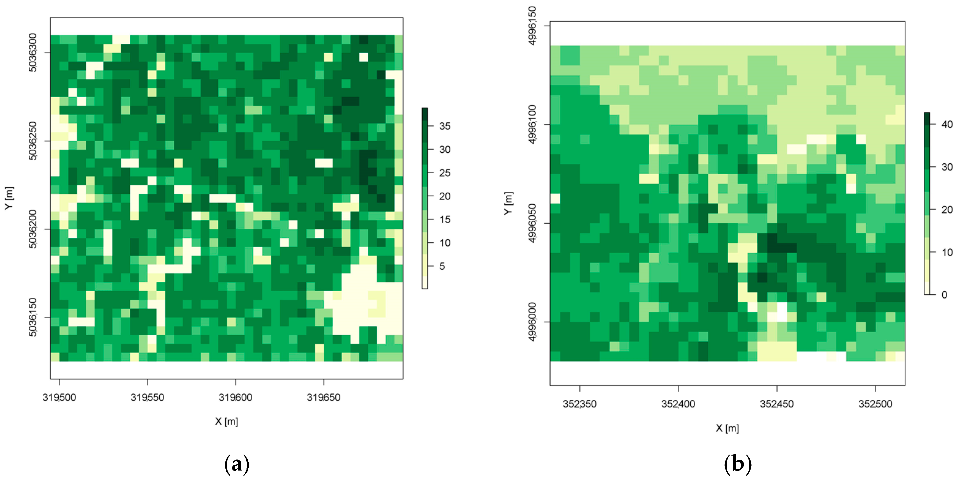
3.2.3. Foliage Indices
3.3. Supporting Services
3.4. Structure Analysis for Cultural Services Assessment
4. Discussion
5. Conclusions
Author Contributions
Funding
Conflicts of Interest
References
- Sasaki, N.; Asner, G.; Knorr, W.; Durst, P.; Priyadi, H.; Putz, F. Approaches to classifying and restoring degraded tropical forests for the anticipated REDD+ climate change mitigation mechanism. iForest Biogeosci. For. 2011, 4, 1–6. [Google Scholar] [CrossRef] [Green Version]
- Pan, Y.; Birdsey, R.A.; Fang, J.; Houghton, R.; Kauppi, P.E.; Kurz, W.A.; Phillips, O.L.; Shvidenko, A.; Lewis, S.L.; Canadell, J.G.; et al. A large and persistent carbon sink in the World’s forests. Science 2011, 333, 988–993. [Google Scholar] [CrossRef] [Green Version]
- Fu, X.; Zhang, Z.; Cao, L.; Coops, N.C.; Goodbody, T.R.; Liu, H.; Shen, X.; Wu, X. Assessment of approaches for monitoring forest structure dynamics using bi-temporal digital aerial photogrammetry point clouds. Remote Sens. Environ. 2021, 255, 112300. [Google Scholar] [CrossRef]
- Badea, O.; Neagu, S.; Bytnerowicz, A.; Silaghi, D.; Barbu, I.; Iacoban, C.; Popescu, F.; Andrei, M.; Preda, E.; Iacob, C.; et al. Long-term monitoring of air pollution effects on selected forest ecosystems in the Bucegi-Piatra Craiului and Retezat Mountains, southern Carpathians (Romania). iForest Biogeosci For. 2011, 4, 49–60. [Google Scholar] [CrossRef] [Green Version]
- Lausch, A.; Borg, E.; Bumberger, J.; Dietrich, P.; Heurich, M.; Huth, A.; Jung, A.; Klenke, R.; Knapp, S.; Mollenhauer, H.; et al. Understanding forest health with remote sensing, part III: Requirements for a scalable multi-source forest health monitoring network based on data science approaches. Remote Sens. 2018, 10, 1120. [Google Scholar] [CrossRef] [Green Version]
- Rasmussen, L.V.; Jepsen, M.R. Monitoring systems to improve forest conditions. Curr. Opin. Environ. Sustain. 2018, 32, 29–37. [Google Scholar] [CrossRef]
- Grafström, A.; Zhao, X.; Nylander, M.; Petersson, H. A new sampling strategy for forest inventories applied to the temporary clusters of the Swedish national forest inventory. Can. J. For. Res. 2017, 47, 1161–1167. [Google Scholar] [CrossRef]
- Ginzler, C.; Hobi, M.L. Countrywide stereo-image matching for updating digital surface models in the framework of the swiss national forest inventory. Remote Sens. 2015, 7, 4343–4370. [Google Scholar] [CrossRef] [Green Version]
- Masek, J.G.; Hayes, D.; Hughes, M.J.; Healey, S.P.; Turner, D.P. The role of remote sensing in process-scaling studies of managed forest ecosystems. For. Ecol. Manag. 2015, 355, 109–123. [Google Scholar] [CrossRef] [Green Version]
- Lechner, A.M.; Foody, G.M.; Boyd, D.S. Applications in remote sensing to forest ecology and management. One Earth 2020, 2, 405–412. [Google Scholar] [CrossRef]
- Boyd, D.; Foody, G. An overview of recent remote sensing and GIS based research in ecological informatics. Ecol. Inform. 2011, 6, 25–36. [Google Scholar] [CrossRef] [Green Version]
- Antonarakis, A.; Richards, K.; Brasington, J. Object-based land cover classification using airborne LiDAR. Remote Sens. Environ. 2008, 112, 2988–2998. [Google Scholar] [CrossRef]
- Yan, W.Y.; Shaker, A.; El-Ashmawy, N. Urban land cover classification using airborne LiDAR data: A review. Remote Sens. Environ. 2015, 158, 295–310. [Google Scholar] [CrossRef]
- García, M.; Riaño, D.; Chuvieco, E.; Danson, F. Estimating biomass carbon stocks for a Mediterranean forest in central Spain using LiDAR height and intensity data. Remote Sens. Environ. 2010, 114, 816–830. [Google Scholar] [CrossRef]
- Popescu, S.C. Estimating biomass of individual pine trees using airborne lidar. Biomass Bioenergy 2007, 31, 646–655. [Google Scholar] [CrossRef]
- Næsset, E. Estimating tree height and tree crown properties using airborne scanning laser in a boreal nature reserve. Remote Sens. Environ. 2002, 79, 105–115. [Google Scholar] [CrossRef]
- Lim, K.S.; Treitz, P.M. Estimation of above ground forest biomass from airborne discrete return laser scanner data using canopy-based quantile estimators. Scand. J. For. Res. 2004, 19, 558–570. [Google Scholar] [CrossRef] [Green Version]
- Chuvieco, E.; Congalton, R.G. Application of remote sensing and geographic information systems to forest fire hazard mapping. Remote Sens. Environ. 1989, 29, 147–159. [Google Scholar] [CrossRef]
- Chuvieco, E.; Kasischke, E.S. Remote sensing information for fire management and fire effects assessment. J. Geophys. Res. Space Phys. 2007, 112. [Google Scholar] [CrossRef] [Green Version]
- Jaboyedoff, M.; Oppikofer, T.; Abellan, A.; Derron, M.-H.; Loye, A.; Metzger, R.; Pedrazzini, A. Use of LIDAR in landslide investigations: A review. Nat. Hazards 2010, 61, 5–28. [Google Scholar] [CrossRef] [Green Version]
- Lim, K.; Treitz, P.; Wulder, M.; St-Onge, B.; Flood, M. LiDAR remote sensing of forest structure. Prog. Phys. Geogr. Earth Environ. 2003, 27, 88–106. [Google Scholar] [CrossRef] [Green Version]
- Jayathunga, S.; Owari, T.; Tsuyuki, S. Evaluating the performance of photogrammetric products using fixed-wing UAV imagery over a mixed conifer-broadleaf forest: Comparison with airborne laser scanning. Remote Sens. 2018, 10, 187. [Google Scholar] [CrossRef] [Green Version]
- Palace, M.W.; Sullivan, F.B.; Ducey, M.J.; Treuhaft, R.N.; Herrick, C.; Shimbo, J.Z.; Mota-E-Silva, J. Estimating forest structure in a tropical forest using field measurements, a synthetic model and discrete return lidar data. Remote Sens. Environ. 2015, 161, 1–11. [Google Scholar] [CrossRef] [Green Version]
- Pascu, I.-S.; Dobre, A.-C.; Badea, O.; Tănase, M.A. Estimating forest stand structure attributes from terrestrial laser scans. Sci. Total. Environ. 2019, 691, 205–215. [Google Scholar] [CrossRef] [PubMed]
- Wulder, M.; Hall, R.J.; Coops, N.; Franklin, S. High spatial resolution remotely sensed data for ecosystem characterization. BioScience 2004, 54, 511–521. [Google Scholar] [CrossRef] [Green Version]
- Lefsky, M.A.; Cohen, W.B.; Parker, G.G.; Harding, D.J. Lidar remote sensing for ecosystem studies. Bioscience 2002, 52, 19–30. [Google Scholar] [CrossRef]
- Holmgren, J.; Nilsson, M.; Olsson, H. Estimation of tree height and stem volume on plots using airborne laser scanning. For. Sci. 2003, 49, 419–428. [Google Scholar]
- McRoberts, R.E.; Tomppo, E.O. Remote sensing support for national forest inventories. Remote Sens. Environ. 2007, 110, 412–419. [Google Scholar] [CrossRef]
- Lefsky, M.; Cohen, W.; Acker, S.; Parker, G.; Spies, T.; Harding, D. Lidar remote sensing of the canopy structure and biophysical properties of Douglas-Fir Western Hemlock Forests. Remote Sens. Environ. 1999, 70, 339–361. [Google Scholar] [CrossRef]
- Pascu, I.-S.; Dobre, A.-C.; Badea, O.; Tanase, M.A. Retrieval of forest structural parameters from terrestrial laser scanning: A Romanian case study. Forests 2020, 11, 392. [Google Scholar] [CrossRef] [Green Version]
- Cabo, C.; Ordóñez, C.; López-Sánchez, C.A.; Armesto, J. Automatic dendrometry: Tree detection, tree height and diameter estimation using terrestrial laser scanning. Int. J. Appl. Earth Obs. Geoinf. 2018, 69, 164–174. [Google Scholar] [CrossRef]
- Othmani, A.; Voon, L.F.L.Y.; Stolz, C.; Piboule, A. Single tree species classification from Terrestrial Laser Scanning data for forest inventory. Pattern Recognit. Lett. 2013, 34, 2144–2150. [Google Scholar] [CrossRef]
- Wallace, L.; Lucieer, A.; Malenovský, Z.; Turner, D.; Vopěnka, P. Assessment of forest structure using two UAV techniques: A comparison of airborne laser scanning and structure from motion (SfM) point clouds. Forests 2016, 7, 62. [Google Scholar] [CrossRef] [Green Version]
- Jarron, L.R.; Coops, N.C.; MacKenzie, W.H.; Tompalski, P.; Dykstra, P. Detection of sub-canopy forest structure using airborne LiDAR. Remote Sens. Environ. 2020, 244, 111770. [Google Scholar] [CrossRef]
- Zheng, G.; Moskal, L.M. Retrieving Leaf Area Index (LAI) using remote sensing: Theories, methods and sensors. Sensors 2009, 9, 2719–2745. [Google Scholar] [CrossRef] [PubMed] [Green Version]
- Hosoi, F.; Omasa, K. Voxel-based 3-D modeling of individual trees for estimating leaf area density using high-resolution portable scanning lidar. IEEE Trans. Geosci. Remote Sens. 2006, 44, 3610–3618. [Google Scholar] [CrossRef]
- Zhang, G.; Hui, G.; Zhao, Z.; Hu, Y.; Wang, H.; Liu, W.; Zang, R. Composition of basal area in natural forests based on the uniform angle index. Ecol. Inform. 2018, 45, 1–8. [Google Scholar] [CrossRef]
- Zhao, Z.; Hui, G.; Hu, Y.; Wang, H.; Zhang, G.; Von Gadow, K. Testing the significance of different tree spatial distribution patterns based on the uniform angle index. Can. J. For. Res. 2014, 44, 1419–1425. [Google Scholar] [CrossRef]
- Lausch, A.; Erasmi, S.; King, D.J.; Magdon, P.; Heurich, M. Understanding forest health with remote sensing, Part I: A review of spectral traits, processes and remote-sensing characteristics. Remote Sens. 2016, 8, 1029. [Google Scholar] [CrossRef] [Green Version]
- Listopad, C.M.; Masters, R.E.; Drake, J.; Weishampel, J.; Branquinho, C. Structural diversity indices based on airborne LiDAR as ecological indicators for managing highly dynamic landscapes. Ecol. Indic. 2015, 57, 268–279. [Google Scholar] [CrossRef]
- Wang, K.; Franklin, S.E.; Guo, X.; Cattet, M. Remote sensing of ecology, biodiversity and conservation: A review from the perspective of remote sensing specialists. Sensors 2010, 10, 9647–9667. [Google Scholar] [CrossRef] [PubMed]
- Kerr, J.T.; Ostrovsky, M. From space to species: Ecological applications for remote sensing. Trends Ecol. Evol. 2003, 18, 299–305. [Google Scholar] [CrossRef]
- Duncanson, L.; Niemann, K.; Wulder, M. Estimating forest canopy height and terrain relief from GLAS waveform metrics. Remote Sens. Environ. 2010, 114, 138–154. [Google Scholar] [CrossRef]
- Lefsky, M.A.; Cohen, W.B.; Acker, S.A.; Spies, T.A.; Parker, G.G.; Harding, D. Lidar remote sensing of forest canopy structure and related biophysical parameters at H.J. Andrews experimental forest, Oregon, USA. In Proceedings of the International Geoscience and Remote Sensing Symposium (IGARSS), Seattle, WA, USA, 6–10 July 1998. [Google Scholar]
- Daily, G.C.; Matson, P.A. Ecosystem services: From theory to implementation. Proc. Natl. Acad. Sci. USA 2008, 105, 9455–9456. [Google Scholar] [CrossRef] [PubMed] [Green Version]
- Gómez-Baggethun, E.; de Groot, R. Natural capital and ecosystem services: The ecological foundation of human society. Ecosyst. Serv. 2010, 30, 105–121. [Google Scholar] [CrossRef]
- Wyatt, T.D.; de Groot, R.S. Valuing nature. Glob. Ecol. Biogeogr. Lett. 1993, 3, 90. [Google Scholar] [CrossRef]
- Costanza, R.; D’Arge, R.; De Groot, R.; Farber, S.; Grasso, M.; Hannon, B.; Limburg, K.; Naeem, S.; O’Neill, R.V.; Paruelo, J.; et al. The value of the world’s ecosystem services and natural capital. Nature 1997, 387, 253–260. [Google Scholar] [CrossRef]
- Balmford, A.; Bruner, A.; Cooper, P.; Costanza, R.; Farber, S.; Green, R.E.; Jenkins, M.; Jefferiss, P.; Jessamy, V.; Madden, J.; et al. Ecology: Economic reasons for conserving wild nature. Science 2002, 297, 950–953. [Google Scholar] [CrossRef] [Green Version]
- De Groot, R.; Brander, L.; van der Ploeg, S.; Costanza, R.; Bernard, F.; Braat, L.; Christie, M.; Crossman, N.; Ghermandi, A.; Hein, L.; et al. Global estimates of the value of ecosystems and their services in monetary units. Ecosyst. Serv. 2012, 1, 50–61. [Google Scholar] [CrossRef]
- Kumar, P. The Economics of Ecosystems and Biodiversity: Ecological and Economic Foundations; Earthscan Publications Ltd.: London, UK, 2013. [Google Scholar]
- Häyhä, T.; Franzese, P.P. Ecosystem services assessment: A review under an ecological-economic and systems perspective. Ecol. Model. 2014, 289, 124–132. [Google Scholar] [CrossRef]
- Bradbeer, J.; Pearce, D. Economic values and the natural world. Geogr. J. 1995, 161, 335. [Google Scholar] [CrossRef]
- Kornatowska, B.; Sienkiewicz, J. Forest ecosystem services-assessment methods. Folia For. Pol. A For. 2018, 60, 248–260. [Google Scholar] [CrossRef] [Green Version]
- Wittmer, H.; Gundimeda, H. The Economics of Ecosystems and Biodiversity for Local and Regional Policy Makers; Routledge: Abingdon-on-Thames, UK, 2011. [Google Scholar]
- Sukhdev, P. The Economics of Ecosystem and Biodiversity; Yale School of Forestry and Environmental Studies: New Heaven, CT, USA, 2011. [Google Scholar]
- IFER. Monitoring and Mapping Solutions. Ltd. FieldMap. 2016. Available online: https://www.youtube.com/watch?v=edBBWh0JyIU&ab_channel=YaleCampus (accessed on 1 March 2021).
- FARO Technologies Inc. Faro Scene; FARO: Lake Mary, FL, USA, 2018. [Google Scholar]
- Hackenberg, J.; Spiecker, H.; Calders, K.; Disney, M.; Raumonen, P. SimpleTree—An efficient open source tool to build tree models from TLS clouds. Forests 2015, 6, 4245–4294. [Google Scholar] [CrossRef]
- RIEGL. LMS-Q680i; RIEGL Laser Measurement Systems GmbH: Horn, Austria, 2012. [Google Scholar]
- Terrasolid Ltd. TerraScan; Terrasolid v021 Ltd.: Helsinki, Finland, 2021. [Google Scholar]
- Axelsson, P. DEM generation from laser scanner data using adaptive TIN models. Int. Arch. Photogramm. Remote Sens. 2000, 33, 110–117. [Google Scholar]
- Brandt, P.; Abson, D.J.; DellaSala, D.A.; Feller, R.; von Wehrden, H. Multifunctionality and biodiversity: Ecosystem services in temperate rainforests of the Pacific Northwest, USA. Biol. Conserv. 2014, 169, 362–371. [Google Scholar] [CrossRef]
- Basuki, T.; van Laake, P.; Skidmore, A.; Hussin, Y. Allometric equations for estimating the above-ground biomass in tropical lowland Dipterocarp forests. For. Ecol. Manag. 2009, 257, 1684–1694. [Google Scholar] [CrossRef]
- Patenaude, G.; Hill, R.; Milne, R.; Gaveau, D.; Briggs, B.; Dawson, T. Quantifying forest above ground carbon content using LiDAR remote sensing. Remote Sens. Environ. 2004, 93, 368–380. [Google Scholar] [CrossRef]
- De Tanago, J.G.; Lau, A.; Bartholomeus, H.; Herold, M.; Avitabile, V.; Raumonen, P.; Martius, C.; Goodman, R.C.; Disney, M.; Manuri, S.; et al. Estimation of above-ground biomass of large tropical trees with terrestrial LiDAR. Methods Ecol. Evol. 2017, 9, 223–234. [Google Scholar] [CrossRef] [Green Version]
- Calders, K.; Newnham, G.; Burt, A.; Murphy, S.; Raumonen, P.; Herold, M.; Culvenor, D.S.; Avitabile, V.; Disney, M.; Armston, J.D.; et al. Nondestructive estimates of above-ground biomass using terrestrial laser scanning. Methods Ecol. Evol. 2014, 6, 198–208. [Google Scholar] [CrossRef]
- He, Q.; Chen, E.; An, R.; Li, Y. Above-ground biomass and biomass components estimation using LiDAR data in a coniferous forest. Forests 2013, 4, 984–1002. [Google Scholar] [CrossRef] [Green Version]
- Brack, C.; Schaefer, M.; Jovanovic, T.; Crawford, D. Comparing terrestrial laser scanners’ ability to measure tree height and diameter in a managed forest environment. Aust. For. 2020, 83, 161–171. [Google Scholar] [CrossRef]
- Roussel, J.R.; Caspersen, J.; Béland, M.; Thomas, S.; Achim, A. Removing bias from LiDAR-based estimates of canopy height: Accounting for the effects of pulse density and footprint size. Remote Sens. Environ. 2017, 198, 1–16. [Google Scholar] [CrossRef]
- Dassot, M.; Colin, A.; Santenoise, P.; Fournier, M.; Constant, T. Terrestrial laser scanning for measuring the solid wood volume, including branches, of adult standing trees in the forest environment. Comput. Electron. Agric. 2012, 89, 86–93. [Google Scholar] [CrossRef]
- Astrup, R.; Ducey, M.J.; Granhus, A.; Ritter, T.; von Lüpke, N. Approaches for estimating stand-level volume using terrestrial laser scanning in a single-scan mode. Can. J. For. Res. 2014, 44, 666–676. [Google Scholar] [CrossRef]
- Ducey, M.J.; Astrup, R.; Seifert, S.; Pretzsch, H.; Larson, B.C.; Coates, K.D. Comparison of forest attributes derived from two terrestrial lidar systems. Photogramm. Eng. Remote Sens. 2013, 79, 245–257. [Google Scholar] [CrossRef]
- Giurgiu, V. Dendrometrie și Auxologie Forestieră; Ceres: Bucharest, Romania, 1979. [Google Scholar]
- McVittie, A.; Hussain, S. The Economics of Ecosystems and Biodiversity—Valuation Database Manual. Available online: http://doc.teebweb.org/wp-content/uploads/2014/03/TEEB-Database-and-Valuation-Manual_2013.pdf (accessed on 1 March 2021).
- Alamgir, M.; Turton, S.M.; Macgregor, C.J.; Pert, P.L. Assessing regulating and provisioning ecosystem services in a contrasting tropical forest landscape. Ecol. Indic. 2016, 64, 319–334. [Google Scholar] [CrossRef]
- Burkhard, B.; Kroll, F.; Nedkov, S.; Müller, F. Mapping ecosystem service supply, demand and budgets. Ecol. Indic. 2012, 21, 17–29. [Google Scholar] [CrossRef]
- De Groot, R.; Alkemade, R.; Braat, L.; Hein, L.; Willemen, L. Challenges in integrating the concept of ecosystem services and values in landscape planning, management and decision making. Ecol. Complex. 2010, 7, 260–272. [Google Scholar] [CrossRef]
- Clark, P.J.; Evans, F.C. Distance to nearest neighbor as a measure of spatial relationships in populations. Ecology 1954, 35, 445–453. [Google Scholar] [CrossRef]
- Vorčák, J.; Merganič, J.; Saniga, M. Structural diversity change and regeneration processes of the Norway spruce natural forest in Babia hora NNR in relation to altitude. J. For. Sci. 2012, 52, 399–409. [Google Scholar] [CrossRef] [Green Version]
- Ajrhough, S.; Maanan, M.; Mharzi Alaoui, H.; Rhinane, H.; El Arabi, E.H. Mapping Forest Ecosystem Services: A Review; International Archives of the Photogrammetry, Remote Sensing and Spatial Information Science—ISPRS Archives; ISPRS: Hannover, Germany, 2019. [Google Scholar]
- Houghton, R.A.; House, J.I.; Pongratz, J.; Van Der Werf, G.R.; Defries, R.S.; Hansen, M.C.; Le Quéré, C.; Ramankutty, N. Carbon emissions from land use and land-cover change. Biogeosciences 2012, 9, 5125–5142. [Google Scholar] [CrossRef] [Green Version]
- Giurgiu, V.; Decei, I.; Draghiciu, D. Metode si Tabele Dendrometrice; Ceres: Bucharest, Romania, 2004. [Google Scholar]
- Eggleston, S.; Buendia, L.; Miwa, K.; Ngara, T.; Tanabe, K. Guidelines for National Greenhouse Gas Inventories: Agriculture, Forestry and Other Land Use; IPCC: Hayama, Japan, 2006. [Google Scholar]
- Lamlom, S.; Savidge, R. A reassessment of carbon content in wood: Variation within and between 41 North American species. Biomass Bioenergy 2003, 25, 381–388. [Google Scholar] [CrossRef]
- Justine, M.F.; Yang, W.; Wu, F.; Tan, B.; Khan, M.N.; Zhao, Y. Biomass stock and carbon sequestration in a chronosequence of pinus massoniana plantations in the upper reaches of the Yangtze River. Forests 2015, 6, 3665–3682. [Google Scholar] [CrossRef] [Green Version]
- Calders, K.; Schenkels, T.; Bartholomeus, H.; Armston, J.D.; Verbesselt, J.; Herold, M. Monitoring spring phenology with high temporal resolution terrestrial LiDAR measurements. Agric. For. Meteorol. 2015, 203, 158–168. [Google Scholar] [CrossRef]
- Danson, F.; Hetherington, D.; Morsdorf, F.; Koetz, B.; Allgower, B. Forest canopy gap fraction from terrestrial laser scanning. IEEE Geosci. Remote Sens. Lett. 2007, 4, 157–160. [Google Scholar] [CrossRef] [Green Version]
- Danson, F.M.; Morsdorf, F.; Koetz, B. Airborne and terrestrial laser scanning for measuring vegetation canopy structure. Laser Scanning Environ. Sci. 2009, 201–219. [Google Scholar] [CrossRef]
- Pascu, I.S.; Dobre, A.-C.; Zamfira, V.; Apostol, E.; Leca, Ș.; Pitar, D.; Apostol, B.; Chivulescu, Ș.; Ciceu, A.; Duro, J.G.; et al. Phenological analysis through the use of multitemporal TLS observations. Rev. Silvic. Cineg. 2020, XXV, 38–45. [Google Scholar]
- Jenkins, R.B. Airborne laser scanning for vegetation structure quantification in a south east Australian scrubby forest-woodland. Austral. Ecol. 2011, 37, 44–55. [Google Scholar] [CrossRef]
- Savastru, D.M.; Zoran, M.A.; Savastru, R.S. Geospatial information for assessment of climate change impact on forest phenology. In Seventh International Conference on Remote Sensing and Geoinformation of the Environment (RSCy2019); International Society for Optics and Photonics: Bellingham, WA, USA, 2019; Volume 11174, p. 1117402. [Google Scholar] [CrossRef]
- Nezval, O.; Krejza, J.; Světlík, J.; Šigut, L.; Horáček, P. Comparison of traditional ground-based observations and digital remote sensing of phenological transitions in a floodplain forest. Agric. For. Meteorol. 2020, 291, 108079. [Google Scholar] [CrossRef]
- Alivernini, A.; Fares, S.; Ferrara, C.; Chianucci, F. An objective image analysis method for estimation of canopy attributes from digital cover photography. Trees 2018, 32, 713–723. [Google Scholar] [CrossRef]
- Stark, S.C.; Leitold, V.; Wu, J.; Hunter, M.; De Castilho, C.V.; Costa, F.R.C.; McMahon, S.M.; Parker, G.; Shimabukuro, M.T.; Lefsky, M.A.; et al. Amazon forest carbon dynamics predicted by profiles of canopy leaf area and light environment. Ecol. Lett. 2012, 15, 1406–1414. [Google Scholar] [CrossRef] [Green Version]
- MacArthur, R.H.; Horn, H.S. Foliage profile by vertical measurements. Ecology 1969, 50, 802–804. [Google Scholar] [CrossRef] [Green Version]
- Swinehart, D.F. The beer-lambert law. J. Chem. Educ. 1962, 39, 333. [Google Scholar] [CrossRef]
- Calloway, D. Beer-lambert law. J. Chem. Educ. 1997, 74, 744. [Google Scholar] [CrossRef] [Green Version]
- Sumida, A.; Nakai, T.; Yamada, M.; Ono, K.; Uemura, S.; Hara, T. Ground-based estimation of leaf area index and vertical distribution of leaf area density in a Betula ermanii forest. Silva Fenn. 2009, 43. [Google Scholar] [CrossRef] [Green Version]
- Stark, S.C.; Enquist, B.; Saleska, S.R.; Leitold, V.; Schietti, J.; Longo, M.; Alves, L.; de Camargo, P.B.; Oliveira, R.C. Linking canopy leaf area and light environments with tree size distributions to explain Amazon forest demography. Ecol. Lett. 2015, 18, 636–645. [Google Scholar] [CrossRef]
- Parker, G.G.; Harding, D.J.; Berger, M.L. A portable LIDAR system for rapid determination of forest canopy structure. J. Appl. Ecol. 2004, 41, 755–767. [Google Scholar] [CrossRef]
- Kamoske, A.G.; Dahlin, K.M.; Stark, S.C.; Serbin, S.P. Leaf area density from airborne LiDAR: Comparing sensors and resolutions in a temperate broadleaf forest ecosystem. For. Ecol. Manag. 2018, 433, 364–375. [Google Scholar] [CrossRef]
- Reid, W.V.; Mooney, H.A.; Cropper, A.; Capistrano, D.; Carpenter, S.R.; Chopra, K.; Zurek, M.B. Ecosystems and Human Well-being-Synthesis: A Report of the Millennium Ecosystem Assessment; Island Press: Washington, DC, USA, 2005. [Google Scholar]
- Haines-Young, R.; Potschin, M. CICES V5. 1. Guidance on the Application of the Revised Structure; Fabis Consulting: Nottingham, UK, 2018. [Google Scholar]
- Haines-Young, R.; Potschin, M. Common international classification of ecosystem services (CICES, Version 4.1). Eur. Environ. Agency 2012, 33, 107. [Google Scholar]
- Li, S.; Wang, T.; Hou, Z.; Gong, Y.; Feng, L.; Ge, J. Harnessing terrestrial laser scanning to predict understory biomass in temperate mixed forests. Ecol. Indic. 2020, 121, 107011. [Google Scholar] [CrossRef]
- Martire, S.; Castellani, V.; Sala, S. Carrying capacity assessment of forest resources: Enhancing environmental sustainability in energy production at local scale. Resour. Conserv. Recycl. 2015, 94, 11–20. [Google Scholar] [CrossRef]
- Street, G.M.; Rodgers, A.R.; Avgar, T.; Fryxell, J.M. Characterizing demographic parameters across environmental gradients: A case study with Ontario moose (Alces alces). Ecosphere 2015, 6, art138. [Google Scholar] [CrossRef] [Green Version]
- Pringle, R.M.; Fox-Dobbs, K. Coupling of canopy and understory food webs by ground-dwelling predators. Ecol. Lett. 2008, 11, 1328–1337. [Google Scholar] [CrossRef]
- Arnold, J.M.; Gerhardt, P.; Steyaert, S.M.; Hochbichler, E.; Hackländer, K. Diversionary feeding can reduce red deer habitat selection pressure on vulnerable forest stands, but is not a panacea for red deer damage. For. Ecol. Manag. 2018, 407, 166–173. [Google Scholar] [CrossRef]
- Ewald, M.; Dupke, C.; Heurich, M.; Muller, J.P.; Reineking, B. LiDAR remote sensing of forest structure and GPS telemetry data provide insights on winter habitat selection of european roe deer. Forests 2014, 5, 1374–1390. [Google Scholar] [CrossRef] [Green Version]
- Martinuzzi, S.; Vierling, L.A.; Gould, W.A.; Falkowski, M.J.; Evans, J.S.; Hudak, A.T.; Vierling, K.T. Mapping snags and understory shrubs for a LiDAR-based assessment of wildlife habitat suitability. Remote Sens. Environ. 2009, 113, 2533–2546. [Google Scholar] [CrossRef] [Green Version]
- Nilsson, M.-C.; Wardle, D.A. Understory vegetation as a forest ecosystem driver: Evidence from the northern Swedish boreal forest. Front. Ecol. Environ. 2005, 3, 421–428. [Google Scholar] [CrossRef]
- Gilliam, F. The ecological significance of the herbaceous layer in temperate forest ecosystems. BioScience 2007, 57, 845–858. [Google Scholar] [CrossRef]
- Hill, R.; Broughton, R. Mapping the understorey of deciduous woodland from leaf-on and leaf-off airborne LiDAR data: A case study in lowland Britain. ISPRS J. Photogramm. Remote Sens. 2009, 64, 223–233. [Google Scholar] [CrossRef]
- Gersom, Z. Mapping the Shrub Layer in a Forest Using LiDAR; Wageningen University and Research Centre: Wageningen, The Netherlands, 2018. [Google Scholar]
- Wing, B.M.; Ritchie, M.W.; Boston, K.; Cohen, W.B.; Olsen, M.J. Individual snag detection using neighborhood attribute filtered airborne lidar data. Remote Sens. Environ. 2015, 163, 165–179. [Google Scholar] [CrossRef]
- Tallis, H.; Ricketts, T.H.; Daily, G.C.; Polasky, S. Natural Capital: Theory and Practice of Mapping Ecosystem Services—Oxford Scholarship. Available online: https://www.amazon.com/Natural-Capital-Practice-Ecosystem-Services/dp/0199589003 (accessed on 1 March 2021).
- Maes, J.; Crossman, N.D.; Burkhard, B. Mapping ecosystem services. In Handbook of Ecosystem Services; Routledge: London, UK, 2018. [Google Scholar]
- Lautenbach, S.; Kugel, C.; Lausch, A.; Seppelt, R. Analysis of historic changes in regional ecosystem service provisioning using land use data. Ecol. Indic. 2011, 11, 676–687. [Google Scholar] [CrossRef]
- Martin, M.; Newman, S.; Aber, J.; Congalton, R. Determining forest species composition using high spectral resolution remote sensing data. Remote Sens. Environ. 1998, 65, 249–254. [Google Scholar] [CrossRef]
- Ørka, H.O.; Dalponte, M.; Gobakken, T.; Næsset, E.; Ene, L.T. Characterizing forest species composition using multiple remote sensing data sources and inventory approaches. Scand. J. For. Res. 2013, 28, 677–688. [Google Scholar] [CrossRef]
- Penman, J.; Gytarsky, M.; Hiraishi, T.; Irving, W.; Krug, T. Guidelines for National Greenhouse Gas Inventories; IPCC: Geneva, Switzerland, 2006. [Google Scholar]
- Pandey, R. Indices for measuring forest ecosystem goods and services contribution to the rural community: A tool for informed decisions. J. Environ. Prof. Sri Lanka 2013, 1, 58. [Google Scholar] [CrossRef] [Green Version]
- Czúcz, B.; Haines-Young, R.; Kiss, M.; Bereczki, K.; Kertész, M.; Vári, Á.; Potschin-Young, M.; Arany, I. Ecosystem service indicators along the cascade: How do assessment and mapping studies position their indicators? Ecol. Indic. 2020, 118, 106729. [Google Scholar] [CrossRef]
- Burkhard, B.; Santos-Martín, F.; Nedkov, S.; Maes, J. An operational framework for integrated Mapping and Assessment of Ecosystems and their Services (MAES). One Ecosyst. 2018, 3, e22831. [Google Scholar] [CrossRef] [Green Version]
- Song, Z.; Seitz, S.; Li, J.; Goebes, P.; Schmidt, K.; Kühn, P.; Shi, X.; Scholten, T. Tree diversity reduced soil erosion by affecting tree canopy and biological soil crust development in a subtropical forest experiment. For. Ecol. Manag. 2019, 444, 69–77. [Google Scholar] [CrossRef]
- Loustau, D.; Granier, A.; Bréda, N. A generic model of forest canopy conductance dependent on climate, soil water availability and leaf area index. Ann. For. Sci. 2000, 57, 755–765. [Google Scholar] [CrossRef]
- Manes, F.; Marando, F.; Capotorti, G.; Blasi, C.; Salvatori, E.; Fusaro, L.; Ciancarella, L.; Mircea, M.; Marchetti, M.; Chirici, G.; et al. Regulating ecosystem services of forests in ten Italian metropolitan cities: Air quality improvement by PM10 and O3 removal. Ecol. Indic. 2016, 67, 425–440. [Google Scholar] [CrossRef]
- Bobiec, A. Living stands and dead wood in the Białowieża forest: Suggestions for restoration management. For. Ecol. Manag. 2002, 165, 125–140. [Google Scholar] [CrossRef]


| Sample Plot | Species | Age [Years] | Silvicultural Interventions | Forest Districts |
|---|---|---|---|---|
| SGT | Sessile oak | 190 | Progressive | Mihăești |
| SGTM | Sessile oak | 190 | Without interventions | Mihăești |
| SFR | Beech | 40 | Thinning | Mihăești |
| SFRM | Beech | 40 | Without interventions | Mihăești |
| SFT | Beech | 120 | Progressive | Mihăești |
| SFTM | Beech | 120 | Without interventions | Mușetești |
| SMR | Norway spruce | 50 | Thinning | Mușetești |
| SMRM | Norway spruce | 50 | Without interventions | Mușetești |
| SMT | Norway spruce | 150 | Progressive | Mușetești |
| SMTM | Norway spruce | 150 | Without interventions | Mușetești |
| Plot | V [m3 ha−1] | dm [cm] | hm [m] | vm [m3] |
|---|---|---|---|---|
| SGT | 444.1 | 21.91 | 20.7 | 0.97 |
| SGTM | 646.4 | 24.15 | 22.36 | 0.90 |
| SFR | 434.6 | 17.81 | 21.9 | 0.37 |
| SFRM | 509.8 | 18.25 | 26.26 | 0.48 |
| SFT | 457.2 | 24.83 | 18.9 | 1.07 |
| SFTM | 622.3 | 25.45 | 19.4 | 1.05 |
| SMR | 345.7 | 17.3 | 17.8 | 0.28 |
| SMRM | 420.1 | 17.45 | 15.8 | 0.29 |
| SMT | 409.5 | 29.29 | 21.6 | 0.90 |
| SMTM | 558.3 | 33.01 | 26.6 | 0.93 |
| Plots | Subplot | Nref | CE | t-Value * | W |
|---|---|---|---|---|---|
| SMTM | 1 | 17 | 1.715 | 1.19 | 0.456 |
| 2 | 11 | 1.829 | 2.19 | 0.432 | |
| 3 | 7 | 1.689 | 2.59 | 0.393 | |
| SGTM | 1 | 20 | 1.558 | 3.12 | 0.563 |
| 2 | 19 | 1.558 | 3.14 | 0.526 | |
| 3 | 25 | 1.825 | 2.68 | 0.510 | |
| SFTM | 1 | 31 | 1.074 | 0.56 | 0.547 |
| 2 | 37 | 1.272 | 1.59 | 0.574 | |
| 3 | 20 | 0.405 | -8.75 | 0.55 | |
| SFRM | 1 | 64 | 1.423 | 1.09 | 0.553 |
| 2 | 55 | 1.283 | 0.91 | 0.515 | |
| 3 | 37 | 1.166 | 0.97 | 0.5 | |
| SMRM | 1 | 92 | 1.269 | 0.4 | 0.532 |
| 2 | 106 | 1.171 | 0.21 | 0.709 | |
| 3 | 87 | 1.025 | 0.04 | 0.548 | |
| SMT | 1 | 46 | 1.751 | 3.17 | 0.531 |
| 2 | 55 | 1.604 | 1.95 | 0.524 | |
| 3 | 38 | 1.429 | 2.41 | 0.561 | |
| SGT | 1 | 39 | 1.321 | 2.7 | 0.545 |
| 2 | 38 | 1.556 | 2.13 | 0.59 | |
| 3 | 35 | 1.575 | 3.65 | 0.558 | |
| SFT | 1 | 26 | 1.551 | 4.46 | 0.635 |
| 2 | 42 | 1.781 | 3.77 | 0.642 | |
| 3 | 36 | 1.549 | 3.34 | 0.643 | |
| SFR | 1 | 71 | 1.309 | 0.68 | 0.715 |
| 2 | 99 | 1.866 | 1.16 | 0.707 | |
| 3 | 76 | 1.628 | 0.95 | 0.725 | |
| SMR | 1 | 102 | 1.301 | 0.38 | 0.719 |
| 2 | 131 | 1.244 | 0.21 | 0.722 | |
| 3 | 147 | 1.252 | 0.37 | 0.723 |
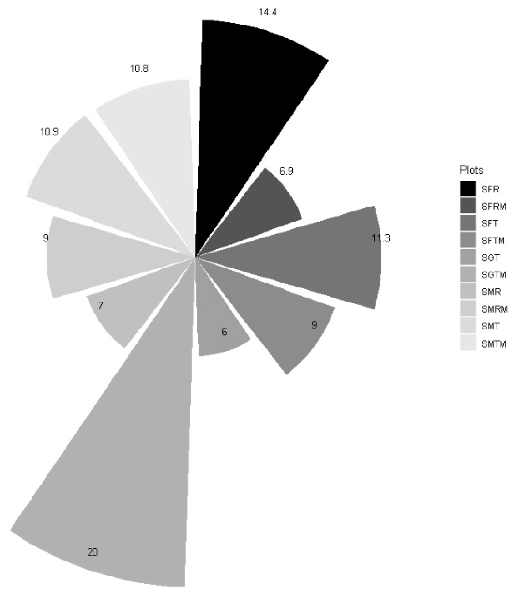
| Plot | V [m3 ha−1] | D 1 [kg m−3] | R 1 | BEF 2 | CF 3 | Carbon Stock [tC·ha−1] |
|---|---|---|---|---|---|---|
| SGT | 444.1 | 584 | 0.22 | 1.4 | 0.48 | 151.88 |
| SGTM | 646.4 | 584 | 0.22 | 1.4 | 0.48 | 221.06 |
| SFR | 434.6 | 545 | 0.19 | 1.4 | 0.46 | 129.66 |
| SFRM | 509.8 | 545 | 0.19 | 1.4 | 0.46 | 152.09 |
| SFT | 457.2 | 545 | 0.19 | 1.4 | 0.46 | 136.40 |
| SFTM | 622.3 | 545 | 0.19 | 1.4 | 0.46 | 185.65 |
| SMR | 345.7 | 353 | 0.2 | 1.3 | 0.51 | 74.68 |
| SMRM | 420.1 | 353 | 0.2 | 1.3 | 0.51 | 90.76 |
| SMT | 409.5 | 353 | 0.2 | 1.3 | 0.51 | 88.47 |
| SMTM | 558.3 | 353 | 0.2 | 1.3 | 0.51 | 120.61 |
Publisher’s Note: MDPI stays neutral with regard to jurisdictional claims in published maps and institutional affiliations. |
© 2021 by the authors. Licensee MDPI, Basel, Switzerland. This article is an open access article distributed under the terms and conditions of the Creative Commons Attribution (CC BY) license (https://creativecommons.org/licenses/by/4.0/).
Share and Cite
Dobre, A.C.; Pascu, I.-S.; Leca, Ș.; Garcia-Duro, J.; Dobrota, C.-E.; Tudoran, G.M.; Badea, O. Applications of TLS and ALS in Evaluating Forest Ecosystem Services: A Southern Carpathians Case Study. Forests 2021, 12, 1269. https://doi.org/10.3390/f12091269
Dobre AC, Pascu I-S, Leca Ș, Garcia-Duro J, Dobrota C-E, Tudoran GM, Badea O. Applications of TLS and ALS in Evaluating Forest Ecosystem Services: A Southern Carpathians Case Study. Forests. 2021; 12(9):1269. https://doi.org/10.3390/f12091269
Chicago/Turabian StyleDobre, Alexandru Claudiu, Ionuț-Silviu Pascu, Ștefan Leca, Juan Garcia-Duro, Carmen-Elena Dobrota, Gheorghe Marian Tudoran, and Ovidiu Badea. 2021. "Applications of TLS and ALS in Evaluating Forest Ecosystem Services: A Southern Carpathians Case Study" Forests 12, no. 9: 1269. https://doi.org/10.3390/f12091269