Soliton Waves in Lossy Nonlinear Transmission Lines at Microwave Frequencies: Analytical, Numerical and Experimental Studies

Abstract

In this paper, we performed analytical, numerical and experimental studies on the generation of soliton waves in discrete nonlinear transmission lines (NLTL) with varactors, as well as the analysis of the losses impact on the propagation of these waves. Using the reductive perturbation method, we derived a nonlinear Schrödinger (NLS) equation with a loss term and determined an analytical expression that completely describes the bright soliton profile. Our theoretical analysis predicts the carrier wave frequency threshold above which a formation of bright solitons can be observed. We also performed numerical simulations to confirm our analytical results and we analyzed the space–time evolution of the soliton waves. A good agreement between analytical and numerical findings was obtained. An experimental prototype of the lossy NLTL, built at the discrete level, was used to validate our proposed model. The experimental shape of the envelope solitons is well fitted by the theoretical waveforms, which take into account the amplitude damping due to the losses in commercially available varactors and inductors used in a prototype. Experimentally observed changes in soliton amplitude and half–maximum width during the propagation along lossy NLTL are in good accordance with the proposed model defined by NLS equation with loss term.

1. Introduction

For electrical engineers, nonlinearity and dispersion are generally undesirable, but a nonlinear transmission line (NLTL) can balance these two effects to generate soliton-like pulses. As stable and localized nonlinear waves, solitons can propagate along NLTL in the form of bell-shaped short-duration voltage pulses [1]. In the last few decades, solitons have become the subjects of numerous studies in various fields of physics and engineering since nature offers various examples of this phenomenon. It is stated in the literature that the first observed soliton was a mono-pulse water wave in a narrow canal where the shallow water possessed both dispersion and nonlinearity [2].

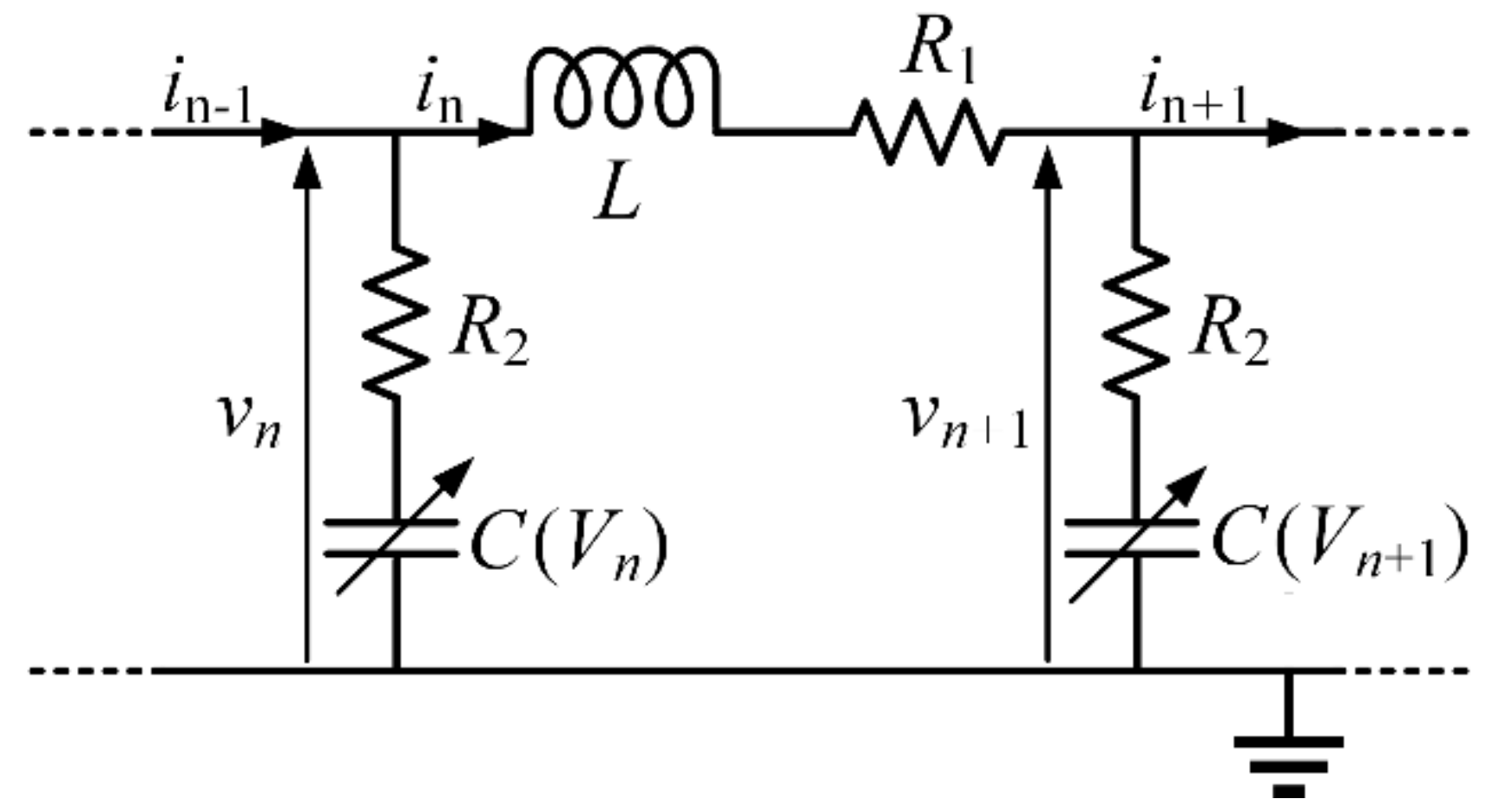
As a nonlinear electronic circuit, the NLTL must contain electrical components with nonlinear permittivity or permeability in order to achieve pulse sharpening [3]. There are generally two possible NLTL designs. The first one uses a ladder network of repeating lumped inductors and capacitors, where the inductors or capacitors are nonlinear in their response to current or voltage, respectively [1,2,3]. For experimental research, this implementation of the equivalent NLTL circuit is most common in which special diodes (varactors or Schottky diodes) are used as nonlinear capacitors placed in shunt form [4]. The second one, more difficult to implement, realizes the NLTL by using a periodically loaded traditional transmission line with lumped varactors [2]. In both NLTL topologies, the dispersion derives from the structural periodicity, while the nonlinearity originates from the varactors—the most commonly used nonlinear components whose capacitance changes with the applied voltage [5]. On the other hand, losses in NLTL are inevitably present due to the finite conductivity of the conductors (resistive losses) as well as the dielectric insulator imperfection (dielectric losses). These losses do not conserve energy and generally have a different effect than the dispersion, which rearranges energy but conserves it [6,7]. Namely, it is known that losses cause a decreases in the amplitude of localized voltage pulses, but the impact of losses has been insufficiently studied in the available literature, especially at microwave frequencies.

In electronics and especially in the microwave domain, NLTLs are of particular interest because of their wide range of possible applications. Since NLTL provides shaping and sharpening of signals, these lines can find important applications for data transmission in high-speed digital circuits [6]. Additionally, due to the possible shrinking in the pulse rise and fall times, NLTL can be applied in high-speed sampling oscilloscopes and other instrumentation for microwave systems [8]. All these studies have shown that NLTL, as a two-port network, requires a high frequency signal at the input to generate a sharp soliton at its output. However, a recent experimental study demonstrated the use of NLTL in an electrical soliton oscillator, as a one-port system, that self-generates the soliton pulses from ambient noise [9]. In addition to NLTL, an amplifier was used in the realization of this soliton oscillator to compensate for losses and to stabilize the oscillations.

The main goal of this paper is to present a new analytical model for the study of the voltage soliton waves in the lossy NLTL with a special focus on the impact of losses on the propagation. The justification of our approach is clearly confirmed by the results of numerical simulations and an experiment that was performed on an NLTL prototype fabricated at the discrete board level. In Section 2, we start with a description of the lossy NLTL model with varactors and we derive a voltage equation for the presented model. In this section, we also determine the parameters of the commercially available varactor used in our study. In Section 3, we provide a detailed theoretical analysis and demonstrate that the NLS equation with loss term can describe the soliton dynamics along the lossy NLTL. The results of the numerical simulations and their comparison with the theoretical predictions are given in Section 4. In Section 5, we describe the experiment and present the results related to the formation of voltage bright solitons, as well as the changes in their amplitude and half–maximum width due to losses. Finally, Section 6 summarizes the key results of this comparative study.

2. Lossy NLTL Model and Voltage Equation

In this study, the lossy NLTL is considered as a nonlinear network of N identical cells of which nth unit cell is shown in Figure 1. Each cell contains a linear inductance L in the series branch, and a nonlinear voltage-dependent capacitance C(V_n) in the shunt branch with V_n being the voltage across it. In addition, two linear resistances R₁ and R₂ are also present in unit cell of NLTL model in order to take into account the component losses. The varactor can serve as the nonlinear capacitor whose typical capacitance–voltage characteristic can be approximated by second-order polynomial function of the voltage across the varactor [10]

$$C\left(V_n\right)=\frac{d{q}_n}{d{V}_n}=C_0\left(1+2\alpha V_n+3\beta V_n^2\right),$$

(1)

where $C_0$ is the characteristic capacitance, parameters $\alpha$ and $\beta$ represent the nonlinear coefficients of the varactor, while $q_n$ is the stored charge in the nth nonlinear capacitor.

Figure 2 shows the variation of the capacitance with the applied reverse voltage for the commercially available varactor (SMV1234–079LF) [11] used in the numerical verification of our theoretical analysis, as well as in the experimental part of this study. The data taken from the varactor datasheet are fitted with Equation (1) and the results are also given in Figure 2. A close agreement between the data (asterisks) and the fit curve (line) was obtained for the following varactor parameters: $C_0=9.8 \mathrm{pF}$, $\alpha =-0.25 V^{-1}$ and $\beta =0.0196 V^{-2}$. These obtained values will be used in numerical simulations for the generation and propagation of solitons along lossy NLTL. Additionally, the varactor’s nonlinear capacitance model’s applicability with Equation (1) confirms its generality.

Voltage Equation

By applying Kirchhoff’s current law at the nth node of the equivalent NLTL circuit, given in Figure 1, we obtain

$$i_{n-1}-i_n=\frac{d{q}_n}{dt}.$$

(2)

On the other hand, applying Kirchhoff’s voltage law to the nth unit cell of the lossy NLTL model, we obtain

$$v_n-v_{n+1}=L\frac{d{i}_n}{dt}+R_1{i}_n.$$

(3)

Taking into account that the voltage across the nonlinear capacitor is $V_n$, the voltage of the nth node can be written as

$$v_n=R_2\left(i_{n-1}-i_n\right)+V_n.$$

(4)

From Equation (3) we have:

$$\begin{gathered} L\frac{d{i}_n}{dt}=v_n-v_{n+1}-R_1{i}_n, \\ L\frac{d{i}_{n-1}}{dt}=v_{n-1}-v_n-R_1{i}_{n-1}. \end{gathered}$$

(5)

Taking the derivative of both sides of Equation (2) and multiplying the whole equation by L, we obtain

$$L\frac{d^2{q}_n}{d{t}^2}=L\frac{d{i}_{n-1}}{dt}-L\frac{d{i}_n}{dt}.$$

(6)

Including Equation (5) in Equation (6), we obtain

$$L\frac{d^2{q}_n}{d{t}^2}=v_{n-1}-2v_n+v_{n+1}+R_1\left(i_n-i_{n-1}\right).$$

(7)

Replacing the expressions for the voltages $v_{n-1}$, $v_n$ and $v_{n+1}$ from Equation (4) to Equation (7) and using the varactor’s nonlinear capacitance model given with Equation (1), we obtain the following discrete nonlinear equation

$$\begin{array}{rr}\left(L{C}_0\frac{d^2}{d{t}^2}+R_1{C}_0\frac{d}{dt}\right)\left(V_n+\alpha V_n^2+\beta V_n^3\right)& =\left(1+R_2{C}_0\frac{d}{dt}\right)\left(V_{n-1}-2V_n+V_{n+1}\right)\\ & +\alpha R_2{C}_0\frac{d}{dt}\left(V_{n-1}^2-2V_n^2+V_{n+1}^2\right)\\ & +\beta R_2{C}_0\frac{d}{dt}\left(V_{n-1}^3-2V_n^3+V_{n+1}^3\right)\end{array}$$

(8)

which describes the envelope soliton propagating along the lossy NLTL considered in this study.

3. Analytical Results

In this paper, the well–known reductive perturbation method [12,13] is used for studying the behavior of short–wavelength envelope electrical solitons. Under the assumption of weak nonlinearity, this method is applied to the characteristic voltage Equation (8) of equivalent lossy NLTL circuit model. To begin this procedure, the envelope spatial and temporal variables are introduced as follows:

$$\xi =\epsilon \left(n-v_{g}t\right), \tau ={\epsilon }^{2}t,$$

(9)

respectively, where $\epsilon$ is the small perturbative parameter, $n$ denotes the NLTL cell number, and $v_g$ represents the group velocity of the wave’s envelope [12]. In the literature [14], it is emphasized that parameter $\epsilon$ measures the smallness of the modulation frequency and the amplitude of the input waves. Now, voltage $V_n$ of nth unit cell at time $t$ can be expanded to a power series of small quantity $\epsilon$ in the following way [15]

$$V_n\left(t\right)={\displaystyle \sum }_{l=1}^{\infty }\left({\displaystyle \sum }_{m=1}^{\infty }{\epsilon }^m{V}_l^{\left(m\right)}\left(\xi ,t\right)\right)e^{il\theta }+c.c.,$$

(10)

where $\theta =kn-\omega t$ represents the rapidly varying phase, $l$ refers to a higher-harmonic wave component and $c.c$. denotes complex conjugate. Additionally, parameters $k$ and $\omega$ are the wavenumber and the angular frequency, respectively.

After substituting the expression of $V_n\left(t\right)$ given with Equation (10) into the discrete nonlinear Equation (8) and using Equation (9), we can transform voltage Equation (8) into a system of equations in different powers of the small perturbative parameter $\epsilon$. Namely, the terms with the same power of $\epsilon$ are collected and set to zero. In that manner, we obtain first-, second- and third-order sets of equations. For the first harmonic ($l=1$), collecting terms at the first-order of the parameter $\epsilon$ leads to the following linear dispersion relation

$${\omega }^2={\omega }_c^2{\sin }^2\left(\frac{k}{2}\right), {\omega }_c=\frac{2}{\sqrt{L{C}_0}},$$

(11)

where ${\omega }_c$ represents the cutoff angular frequency. In Figure 3, the dispersion curve is given, defined by the Equation (11), for the lossy NLTL under study. This curve shows the evolution of frequency $f=\omega /2\pi$ as a function of the wavenumber $k$, which is taken in the Brillouin zone, $0\le k\le \pi$ [16]. For the characteristic capacitance of the varactor $C_0=9.8 \mathrm{pF}$ and linear inductance $L=2 \mathrm{nH}$, the cutoff frequency of $f_{max}\cong 2.28 \mathrm{GHz}$ was obtained. Furthermore, based on the linear dispersion relation given by Equation (11), the corresponding group velocity $v_g$ is determined by the following expression

$$v_g=\frac{\partial \omega }{\partial k}=\frac{1}{\sqrt{L{C}_0}}\cos \left(\frac{k}{2}\right).$$

(12)

On the other hand, for the first harmonic collecting terms at the third-order of the parameter $\epsilon$, we obtain the following equation going over to continuum approximation

$$i\frac{\partial V}{\partial \tau }-\frac{\omega }{8}\frac{{\partial }^{2}V}{\partial {\xi }^2}+{\alpha }^2\omega \left(\frac{3\beta }{2{\alpha }^2}+\frac{{\omega }_c^2}{{\omega }^2}-2\right){\left|V\right|}^{2}V=-i\left(\frac{R_1}{2L}+\frac{2R_2}{L}{\sin }^2\left(\frac{k}{2}\right)\right)V.$$

(13)

Thus, propagation the time–space voltage waves along the lossy NLTL can be modeled by a nonlinear Schrödinger (NLS) equation incorporating a linear loss term [17,18]

$$i\frac{\partial V}{\partial \tau }+P\left(\omega \right)\frac{{\partial }^{2}V}{\partial {\xi }^2}+Q\left(\omega \right){\left|V\right|}^{2}V=-i\mathsf{\Gamma }V,$$

(14)

where are, respectively the dispersion, nonlinearity and dissipation coefficients given by:

$$P\left(\omega \right)=-\frac{\omega }{8}, Q\left(\omega \right)={\alpha }^2\omega \left(\frac{3\beta }{2{\alpha }^2}+\frac{{\omega }_c^2}{{\omega }^2}-2\right), \mathsf{\Gamma }=\frac{R_1}{2L}+\frac{2R_2}{L}{\sin }^2\left(\frac{k}{2}\right).$$

(15)

It is clear from Equation (15) that the sign of the dispersion coefficient $P\left(\omega \right)$ is always negative. However, the sign of the nonlinearity coefficient $Q\left(\omega \right)$ depends on the nonlinear characteristics of the voltage-dependent capacitance, as well as the carrier wave angular frequency, $\omega$. Therefore, the focusing or the defocusing effect and the corresponding generation of bright or dark solitons [19] in lossy NLTL can be described and understood by means of the NLS Equation (14) with losses. Namely, the sign of the product $PQ$ can be positive or negative, which leads to formation of a bright soliton ($PQ>0$) or a dark soliton ($PQ<0$), respectively [12,13]. Figure 4 shows the wavenumber (frequency) dependence of the product $PQ$ for the lossy NLTL under study. Namely, two different regimes are observed: a dark soliton regime ($PQ<0$) at low frequencies (light green region), and bright soliton regime ($PQ>0$) at high frequencies (dark green region). According to determined parameters of commercially available varactor (SMV1234–079LF) [11], see Figure 2, and commercial linear inductor (MLG1005S2N0BTD25) [20] used in this study, our analytical results predict that the threshold value of the carrier wave frequency is $f_{min}\cong 1.64 \mathrm{GHz}$, above which a formation of bright solitons will occur. Below, we focus on the numerical and experimental study of bright soliton generation and its propagation at higher frequencies ($f_{min}<f<f_{max})$ in accordance with the results of our theoretical analysis.

In the absence of losses ($\mathsf{\Gamma }=0$), Equation (13) reduces to the standard NLS equation, which possesses numerous symmetries and respective conservation laws such as the total pulse intensity and total energy [18]. A well-known analytical bright soliton solution of the standard NLS equation for the envelope function $V$ is given with the following expression [17]

$$V\left(\xi ,\tau \right)=A_0\sec \mathrm{h}\left(A_0\sqrt{\frac{Q}{2P}}\xi \right)e^{i\frac{A_0^{2}Q}{2}\tau },$$

(16)

where $A_0$ denotes a real amplitude that depends on the initial conditions. Furthermore, from Equation (16), it is obtained that the spatial width of the soliton defined at half maximum can be determined as [16]

$$W_{FWHM}=2\sqrt{\frac{2P}{A_0^{2}Q}}{\sec \mathrm{h}}^{-1}\left(\frac{1}{2}\right).$$

(17)

It is obvious that the increase in nonlinearity causes greater localization of soliton waves and the area covered by the envelope function $V$, given by Equation (16), remains preserved. For example, if the carrier wave frequency $f=2 \mathrm{GHz}$, which is in the previous determined frequency range $f_{min}<f<f_{max}$ for bright soliton formation in lossy NLTL under study, one finds $P\cong -1.58·{10}^9 \mathrm{rad}/\mathrm{s}$ and $Q\cong -0.32·{10}^9 {\mathrm{V}}^{-2}\mathrm{rad}/\mathrm{s}$ with the use of known varactor and inductor parameters. Theoretically, it provides that the width at half maximum calculated by Equation (17) is $W_{FWHM}\cong 7 \mathrm{cells}$. This result indicates that the degree of localization ensures that the exploited continuum approximation can be fairly justified.

On the other hand, when losses are present in the NLTL ($\mathsf{\Gamma }>0$), it is necessary to include the impact of a dissipation on the soliton wave dynamics. According to soliton perturbation theory, the losses do not affect the velocity of the soliton but its amplitude, which becomes a decaying function of time [17]. Specifically, the amplitude of the bright soliton, defined by the lossy NLS Equation (14), will decrease exponentially as $e^{-2\mathsf{\Gamma }\tau }$ [18]

$$V\left(\xi ,\tau \right)=A_0{e}^{-2\mathsf{\Gamma }\tau }\sec \mathrm{h}\left(A_0\sqrt{\frac{Q}{2P}}{e}^{-2\mathsf{\Gamma }\tau }\xi \right)e^{i\frac{A_0^{2}Q}{8}\mathsf{\Gamma }\left(1-e^{-4\mathsf{\Gamma }\tau }\right)},$$

(18)

while its spatial width increases exponentially as $e^{2\mathsf{\Gamma }\tau }$.

Regarding a modulational instability, study [16] showed that a plane-wave solution of NLS Equation (14) is modulationally stable for $PQ<0$. On the other hand, for $PQ>0$, the system can be modulation unstable if the frequency of the perturbation $F$ satisfies the following condition

$$F<F_{cr}=\frac{v_g{K}_{cr}}{2\pi },$$

(19)

where $K_{cr}$ is the corresponding wavenumbers determined by

$$K_{cr}=A_0\sqrt{\frac{2Q}{P}}.$$

(20)

In this case, the modulation increases as time progresses and the continuous wave breaks into a periodic pulse or envelope soliton train. With the use of the lossy NLTL parameters, the theoretical frequency of the envelope modulation for $A_0=1$ V lies in the instability domain $0<F<0.73 \mathrm{GHz}$, predicted by Equation (19). Furthermore, in a mechanical analogue of NLS equation with viscous dissipation, it has been experimentally demonstrated that dissipation generally prevents modulational instability [21]. Namely, modulational instability might still occur, but losses can stop the growth of perturbations before nonlinear interactions become significant. In this case, if the perturbations are small enough initially, then they never grow large enough for nonlinear interactions to become important.

4. Results of Numerical Simulations

In order to verify our theoretical predictions, numerical simulations were performed on a lossy NLTL with 30 identical cells, see Figure 1. For this purpose, we considered that each NLTL cell consists of varactors (SMV1234–079LF) [11] with an average serial loss of $R_2=1 \mathsf{\Omega }$, and fixed linear SMD inductors $L=2 \mathrm{nH}$ (MLG1005S2N0BTD25) [20] with an average loss of $R_1=0.8 \mathsf{\Omega }$. Additionally, the varactor parameters used in our numerical analysis were determined by fitting the data taken from the varactor datasheet, see Figure 2. A circuit simulator is implemented in the MATLAB software package using a well–known finite-difference method in the time domain.

For an input pulse of amplitude 1 V and a carrier wave frequency $f=2 \mathrm{GHz}$ selected in the passband of the NLTL, see Figure 4, the numerically obtained envelope waveform is presented in Figure 5. It is obvious that a bright soliton is formed, preserving its shape, which is in good agreement with our theoretical predictions since the product of the dispersion and nonlinearity coefficients is positive for the parameters of the NLTL and accordingly the bright soliton should occur. The direct comparison of analytical and numerical results for envelope soliton at the 20th cell of the lossy NLTL is given in Figure 6. Evidently, a good match between the obtained waveforms confirms that the lossy NLS approximation, defined by Equation (14), is the suitable model for describing the generation and propagation of soliton waves along NLTL with losses.

Based on the obtained numerical results shown in Figure 5, the impact of losses present in NLTL on the soliton amplitude is obvious and in agreement with our theoretical predictions. According to soliton perturbation theory [16,17], the amplitude of the envelope soliton is an exponentially decreasing function of time, see Equation (18). To confirm these predictions, we have studied in detail how the amplitude of the envelope bright soliton with carrier wave frequency $f=2 \mathrm{GHz}$ decays along the NLTL. The obtained results are illustrated in Figure 7. These data were fitted with an exponential function and close values for the damping constant were calculated. Namely, according to our theoretical predictions and numerical results, the damping constants are $\gamma =0.0126 {\mathrm{cell}}^{-1}$ and $\gamma =0.0141 {\mathrm{cell}}^{-1}$, respectively. These values are in good agreement, as well as with the experimental results ($\gamma =0.0159 {\mathrm{cell}}^{-1}$) that will be discussed in the section below.

5. Experimental Results

In order to validate our analytical and numerical results, experiments were carried out on an NLTL prototype with 30 identical cells, which was fabricated at the discrete board level, as shown in the inset of Figure 8. In this prototype, commercially available SMD linear inductors (MLG1005S2N0BTD25) [20] and varactors (SMV1234–079LF) [11], which serve as nonlinear capacitances, were used. The parameter values of these components are the same as the parameters used in the analytical and numerical study. The fabricated NLTL prototype was fed by a signal generator (Agilent E4438C ESG), and soliton waveforms were analyzed using a high-performance $6 \mathrm{GHz}$ oscilloscope (Infiniium DSO90604A) with probes which have high impedance and small capacitance in order to avoid parasitic reflections. Generally, the main experimentally adjustable parameters are: the pulse frequency, amplitude and width. In this experimental study, a voltage pulse of amplitude $V_0=1 \mathrm{V}$ and frequency $f=2 \mathrm{GHz}$ was applied at the input of the NLTL.

Figure 8 displays the measured voltage response at three different NLTL nodes. Specifically, the upper, middle and bottom traces correspond to the response at nodes 10, 20 and 30, respectively. It is obvious that the bright soliton profile possesses a well-defined envelope and remains localized as it travels along NLTL even though it loses some of its energy due to dissipation. The measured values of the amplitude and half–maximum width at node 10 were $V_0=0.85 \mathrm{V}$ and $W_{FWHM}=98 \mathrm{ps}$, respectively, whereas the corresponding values at node 30 (the end of the NLTL) were $V_0=0.64 \mathrm{V}$ and $W_{FWHM}=124 \mathrm{ps}$, respectively. This obtained decrease in the amplitude of the envelope soliton is well-matched with theoretical analysis and results of numerical simulations, as can be seen in Figure 7. The small discrepancy is most likely caused by additional losses in conductors which are not included in the NLTL model, as well as the fact that the parameter values of components vary according to their tolerances. Additionally, the bright soliton with higher amplitude has smaller half-maximum width, which is in good agreement with our analytical result given by the Equations (17) and (18). This is a clear affirmation of our theoretical prediction that the proposed model defined by NLS Equation (14) with losses is able to excellently predict the soliton waveforms.

6. Conclusions

In this study, we have reported analytical, numerical, and experimental results of propagation characteristics of soliton waves in the lossy NLTL, loaded periodically with linear series inductors and shunt varactors used as nonlinear capacitors. Starting from Kirchhoff’s laws and then applying the reductive perturbation method, we have demonstrated that the NLS equation with loss term can describe the soliton dynamics along the lossy NLTL. Our analytical analysis allowed us to correctly identify the frequency range in which bright solitons were experimentally observed. Further, with the help of the determined analytical solution, which completely describes the bright soliton profile, it is possible to choose suitable parameters of NLTL to satisfy the required application. Using the parameter values of commercially available components which were utilized to realize the NLTL prototype, we have also performed numerical simulations in order to verify our theoretical predictions. The good agreement between the analytical and numerical waveforms clearly justifies the utility of our approach (NLS equation with loss term) for the study of voltage soliton waves in the lossy NLTL. Experiments were carried out on the NLTL prototype with 30 identical cells, built at the discrete level, and it was noticed that the experimentally obtained soliton profiles matched very well with the theoretically predicted waveforms. During the propagation of the bright solitons along lossy NLTL, experimental results showed that the soliton amplitude decreases and half-maximum width increases due to the losses in commercially available varactors and inductors used in this study. These results suggest that the losses must be reduced in order to improve the propagation of voltage solitons.