Unsupervised Neural Networks for Identification of Aging Conditions in Li-Ion Batteries

Abstract

This paper explores a new methodology based on data-driven approaches to identify and track degradation processes in Li-ion batteries. Our goal is to study if it is possible to differentiate the state of degradation of cells that present similar aging in terms of overall parameters (similar remaining capacity, state of health or internal resistance), but that have had different applications or conditions of use (different discharge currents, depth of discharges, temperatures, etc.). For this purpose, this study proposed to analyze voltage waveforms of cells obtained in cycling tests by using an unsupervised neural network, the Self-Organizing Map (SOM). In this work, a laboratory dataset of real Li-ion cells was used, and the SOM algorithm processed battery cell features, thus carrying out smart sensing of the battery. It was shown that our methodology differentiates the previous conditions of use (history) of a cell, complementing conventional metrics such as the state of health, which could be useful for the growing second-life market because it allows for determining more precisely the state of disease of a battery and assesses its suitability for a specific application.

1. Introduction

The use of lithium batteries for energy storage has had a large growth in the last decade, becoming standard for both electric vehicles (EV) and hybrid vehicles (HEV), as well as for stationary storage systems. For this reason, the demand for critical materials such as cobalt, graphite or lithium is increasing [1].

The growth in lithium demand for battery production already accounted for 46% of all global production in 2017 [2]. The global lithium production has grown at a 20% rate per year since 2000 [3], and it is expected that in 2025 the market for second-life batteries will exceed 95 GWh only from EV [4]. This growth rate makes it necessary to design a full lifecycle, from manufacturing to the reuse and recycling processes.

In the second-life market there are three levels of reuse: pack, module and cell [5]. Battery cells can be used in applications related to stationary energy storage systems (SESSs), where the battery reuse extends their lifespan by 40% [6]. In addition, they can be ideal for frequency containment and restoration reserves (FCR and FRR) in on-grid regulation [7], or in the residential sector to support solar energy production [8].

The value-chain of Li-ion batteries after being used in their main application can pose different use scenarios, such as direct reuse, second-use or recycling. However, the current second-life market only considers the reuse of the complete pack to be profitable due to economic criteria and the difficulty of determining the quality of the extracted cells [9]. Nowadays, the second-life batteries come from automotive applications, where battery packs are manufactured. The mechanical difficulty of disassembling these packs makes the material and labor costs rise significantly. Some authors are already studying the possibilities to find an alternative source of second-life cells, for example, Li-ion cells rescued from notebook batteries, whose capacities continue to exceed 70% nominal [10].

As a contribution to this matter, this article presents a new technique with the objective of differentiating the aging of the cells coming from different unknown applications. A large number of variables are used for determining battery aging. All cells have a calendar-life degradation [11] which is not related to their use and will have a long-term impact that is the same for all the batteries produced in the same batch. However, there are many other factors that depend on the application for which the batteries have been previously used: temperature, charging and discharging current profiles, and voltage range or power peaks, among others. These factors are further defined in [12,13].

Aging entails a variation of the internal composition of the cell, affecting the electrochemical reactions that take place, reducing its capacity and, from an electrical point of view, increasing its internal resistance. These effects make the modeling of a battery throughout its life cycle a highly nonlinear problem that is not yet well resolved.

The most common metric introduced to define the state of a battery is the State of Health (SoH), which returns a percentage (0–100%) based on a definable quotient for several characteristics of the model (capacities, impedances, etc.), calculable by using a wide variety of well-known techniques, grouped in [14,15]. Some authors recently studied physical correlations to define the actual SoH, such as [16,17]. Others have proposed the study of the incremental capacity curves from laboratory analysis [18,19].

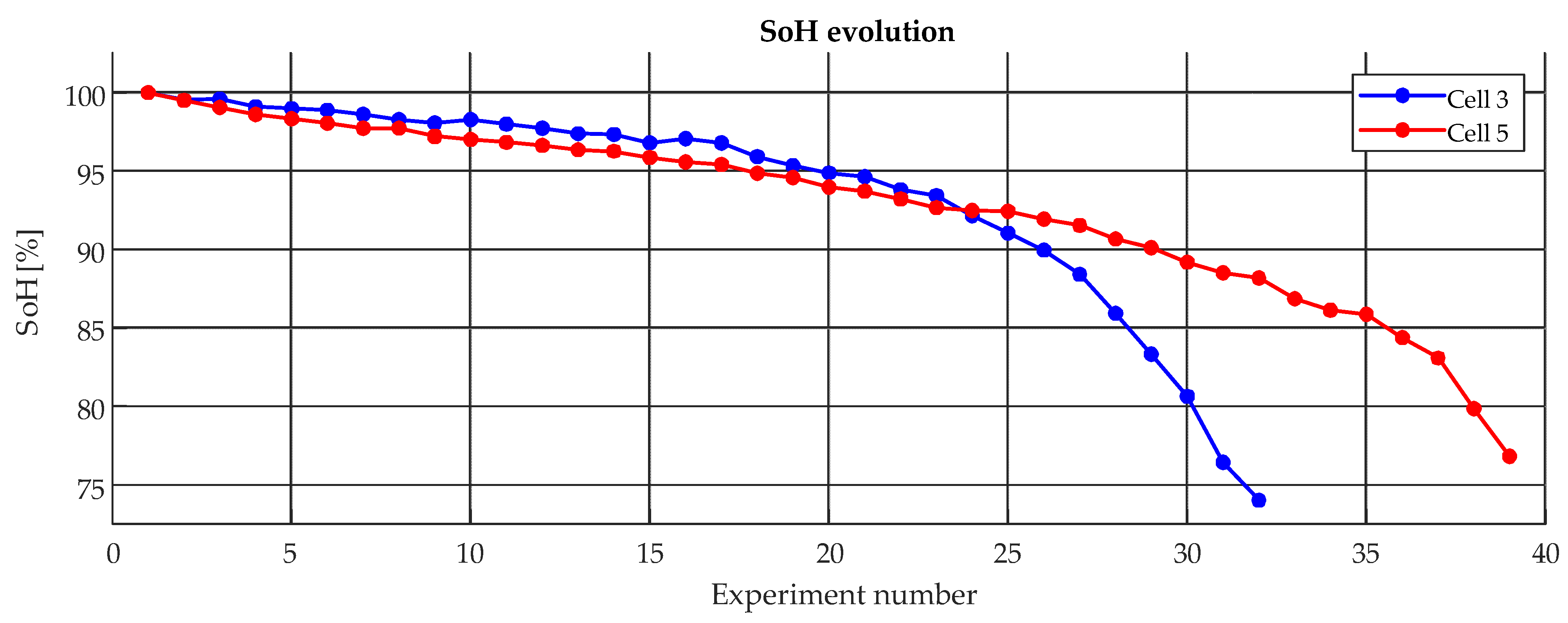
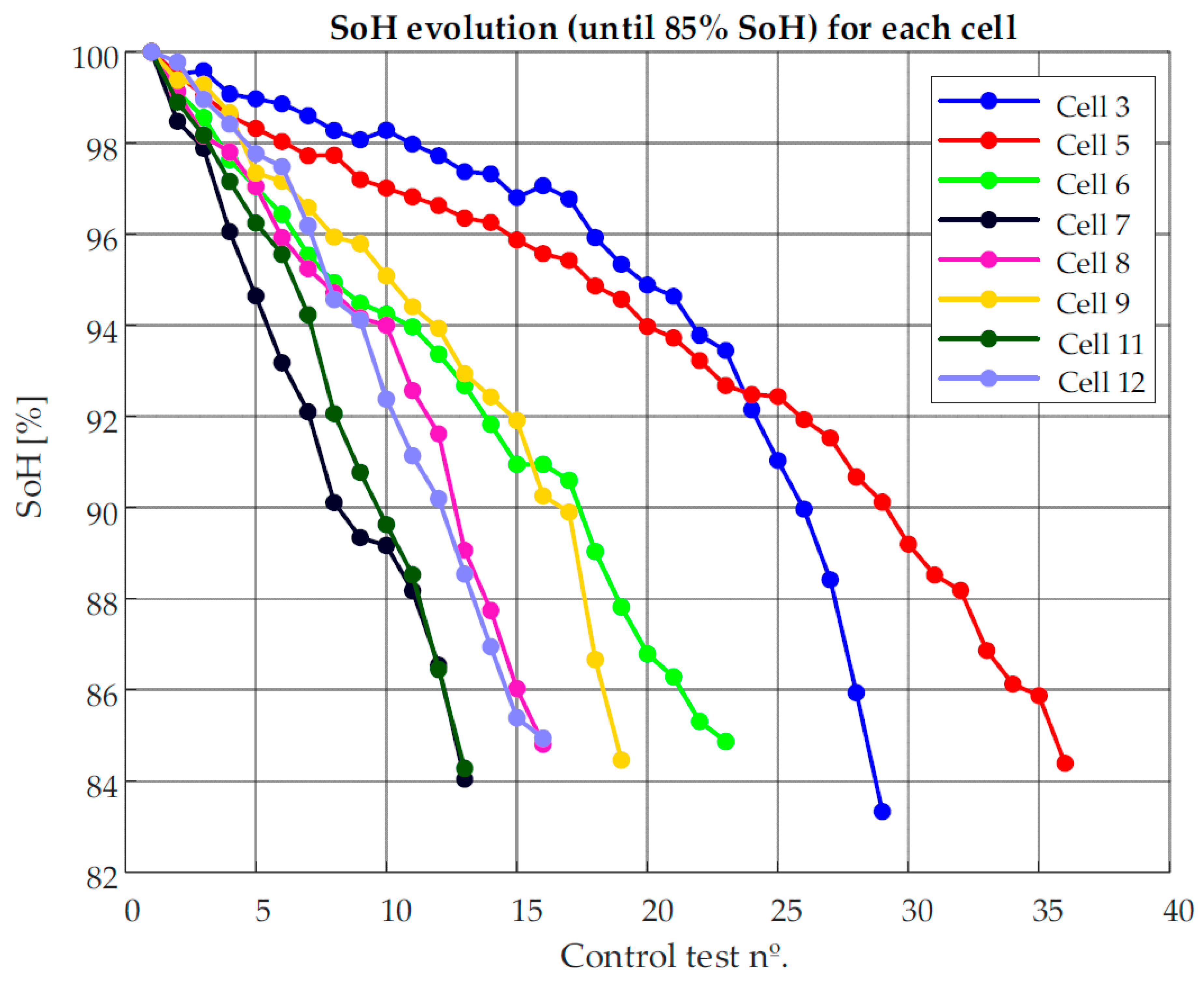
However, this classic view of aging does not take into account the non-linearity of the health status of cells nor the influence of SoH in other states of function, such as the expected capacity fade, the maximum obtainable power, self-heating and other known issues of a degraded cell. Thus, it has been experimentally observed that two cells can have the same SoH at a certain point in their life cycle, but they can have a totally different aging curve (Figure 1) due to different applications or uses that they have previously had (discharge currents, temperatures or depth of discharge).

More modern approaches use data-driven techniques to estimate aging, which are reviewed in [20,21]. There are similar techniques based on Support Vector Machines (SVM) trained with data from previous uses, such as [22].

Newer techniques such as LSTM neural networks and deep learning are used in online prediction by using inputs such as capacity and temperature [23,24].

Other authors have proposed capacity estimation methods based on complete charging curves using Gaussian Process Regression (GPR), such as [25,26].

Particle filtering is another widely applied method for degradation estimation, as proposed in [27]. Capacity analysis has also been studied, calculating degradation through the charge-discharge efficiency calculation [28]. Finally, [29] proposed the use of Principal Component Analysis (PCA), perhaps the proposal most similar to ours, but with the important limitation that PCA is a linear technique.

The aim of our study consists of developing a methodology for cell aging estimation complementary to the classical definition of SoH, where only battery capacity is considered. Thus, a new methodology based on data-driven techniques is presented for contributing to determine the state of degradation of cells with different conditions of use but similar degradation (i.e., with similar remaining capacity, SoH or internal resistance). This new methodology analyzes voltage waveforms obtained in cycling tests by using an unsupervised neural network, the Self-Organizing Map (SOM). It will be shown that this methodology allows the differentiation of previous conditions of use (history) of a cell in an unsupervised and visual way, complementing conventional metrics such as the SoH.

A first version of this methodology was previously explored in [30]. However, the results were not as successful as expected due to the limited dataset used and the lack of a feature extraction stage. In this new study, a different dataset is used, feature extraction is incorporated, and new quantitative metrics are proposed.

In summation, these are the original contributions of this article:

• A new methodology for cell aging analysis based on the SOM is proposed.
• A feature extraction methodology based on polynomials is studied.
• An original database crafted for aging studies, provided by an external OEM, is used.
• Three new metrics to evaluate trajectories onto the SOM are proposed.
• New D-matrix 3D-map representation, including trajectories with their quantization errors, is used.
• Some application examples for the proposed technique are given.

This paper is organized as follows. In Section 2, the methodology is presented. First, the self-organizing map neural model is introduced, then the dataset used in our work is described, the feature extraction process is explained, and new metrics are defined. In Section 3, the results achieved by our methodology are presented, including two types of visualizations for the SOM. In Section 4, two applications of our methodology are described. Finally, in Section 5 the conclusions of our work are provided.

2. Methodology

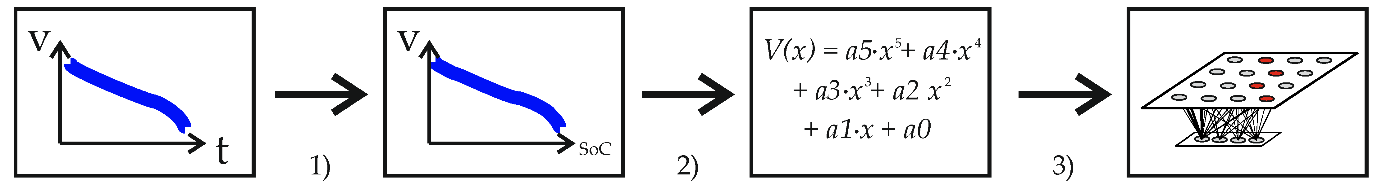
Our methodology consisted of three steps: (1) voltage-time curves were obtained and normalized, (2) some features were extracted, (3) features were processed by means of self-organizing maps, which were analyzed by visual inspection and by using the proposed metrics. A schematic for the technique is shown in Figure 2.

2.1. Self-Organizing Maps

A Self-Organizing Map (SOM) [31,32] is an unsupervised neural model used for pattern recognition, cluster search and database visualization. Unlike other unsupervised techniques (clustering, PCA, etc.), the SOM is nonlinear and allows for monitoring the evolution of a system.

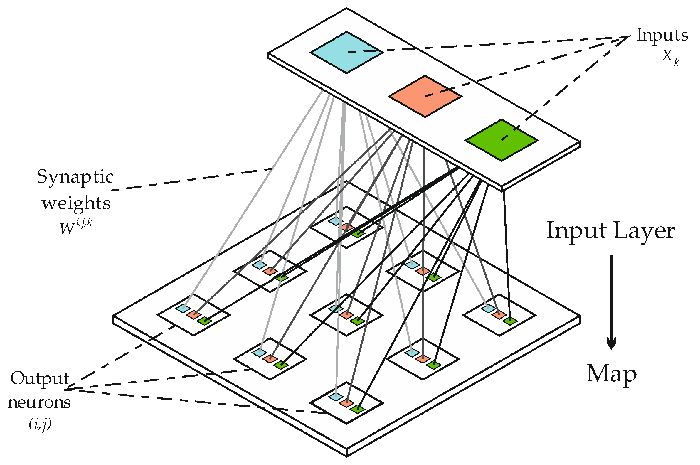
A SOM consists of an input layer and an output layer (map), which is a rectangular array of neurons (Figure 3). It has two modes of operation: training and inference. Given a map of nx × ny neurons and an input layer of n variables x_k (1 ≤ k ≤ n), each neuron (i, j) stores a weight vector w_ij of n components (Figure 3). In inference, each neuron (i, j) computes the similarity between the vector of inputs x_k and the vector of weights w_ijk; the Euclidean distance is normally used:

$$d^2(w_{ij},x)={\displaystyle \sum _{k=1}^n{(w_{ijk}-x_k)}^2}$$

(1)

The neuron that minimizes the distance to the input vector is considered to have recognized the input pattern, called the winning neuron or best-matching unit (BMU).

In the training phase, the synaptic weights are adjusted. The weights start with a random value, in each iteration t an input vector x(t) is presented and the process of looking for the winning neuron is carried out, as described in the inference phase. The weights of the winning neuron and those around it (neighborhood) are adjusted by:

$$\Delta w_{ijk}(t)=\epsilon (t)\cdot \left(x_k(t)-w_{ijk}(t)\right)$$

(2)

where ε(t) is the learning rate, which decreases over time:

$$\epsilon (t)={\epsilon }_0+({\epsilon }_f-{\epsilon }_0)\frac{t}{t_f}$$

(3)

where ε₀ represents the initial learning rate (ε₀ < 1.0), ε_f is the final rate (ε_f ≈ 0.01), t_f is the estimated number of iterations to reach ε_f.

The neuron weights can be updated online (example by example) or after processing a batch of examples; in our work, the batch algorithm was used. On the other hand, in many applications the input variables have very different variation ranges so they are usually normalized; in our work, the input variables were normalized to mean 0 and variance 1.

To quantify the quality of the trained map, two metrics are available, as can be seen in [33]. The quantization error (qe) measures the resolution of the trained map and is calculated as the mean of the Euclidean distances between every input vector, x_i, and the neuron vector for which this distance is minimized (BMU), $m_{x_i}$, for all input samples, N, as it is shown in Equation (4):

$$qe=\frac{1}{N}{\displaystyle \sum _{i=1}^N\Vert x_i-m_{x_i}\Vert }$$

(4)

On the other hand, the SOM generates a non-linear projection of the multidimensional input space onto the two-dimensional map, allowing the visualization of the structure of the dataset and possible clusters. The topographic error (te) quantifies the topology preservation by computing the proportion of all input vectors for which the first BMU and the second BMU (the second neuron that minimizes the distance between the input vector and its weights) are not adjacent:

$$te=\frac{1}{N}{\displaystyle \sum _{i=1}^{N}u(x_i)}$$

(5)

where u() acquires the value 1 when the two first BMUs for the input vector x_i are adjacent and 0 otherwise.

A visualization tool called a U-matrix [31,32] is frequently used for drawing borders between the different clusters that may be presented on the SOM. The U-matrix procedure generates a new map that visualizes the Euclidean distance between neighboring neurons in gray levels, but the dimensions of this new map are almost double those of the initial SOM since it is built from Euclidean distances computed for pairs of adjacent neurons: a nx × ny SOM yields a (2nx − 1) × (2ny − 1) U-matrix map. In this work, the so-called D-matrix is used as a visualization tool instead because the D-matrix averages the distances between neighboring nodes of the U-matrix to generate a map of mean distances that has the same dimensions as the original SOM (nx × ny).

Finally, once a SOM has been trained, it is used in inference mode. In our case (Section 3 and Section 4), by presenting data of a cell, the BMU given by Equation (1) indicates its current state (cell diagnosis). By providing a data series from a cell, the consecutive BMUs describe a trajectory on the map that shows the evolution of the state of that battery cell.

2.2. Database

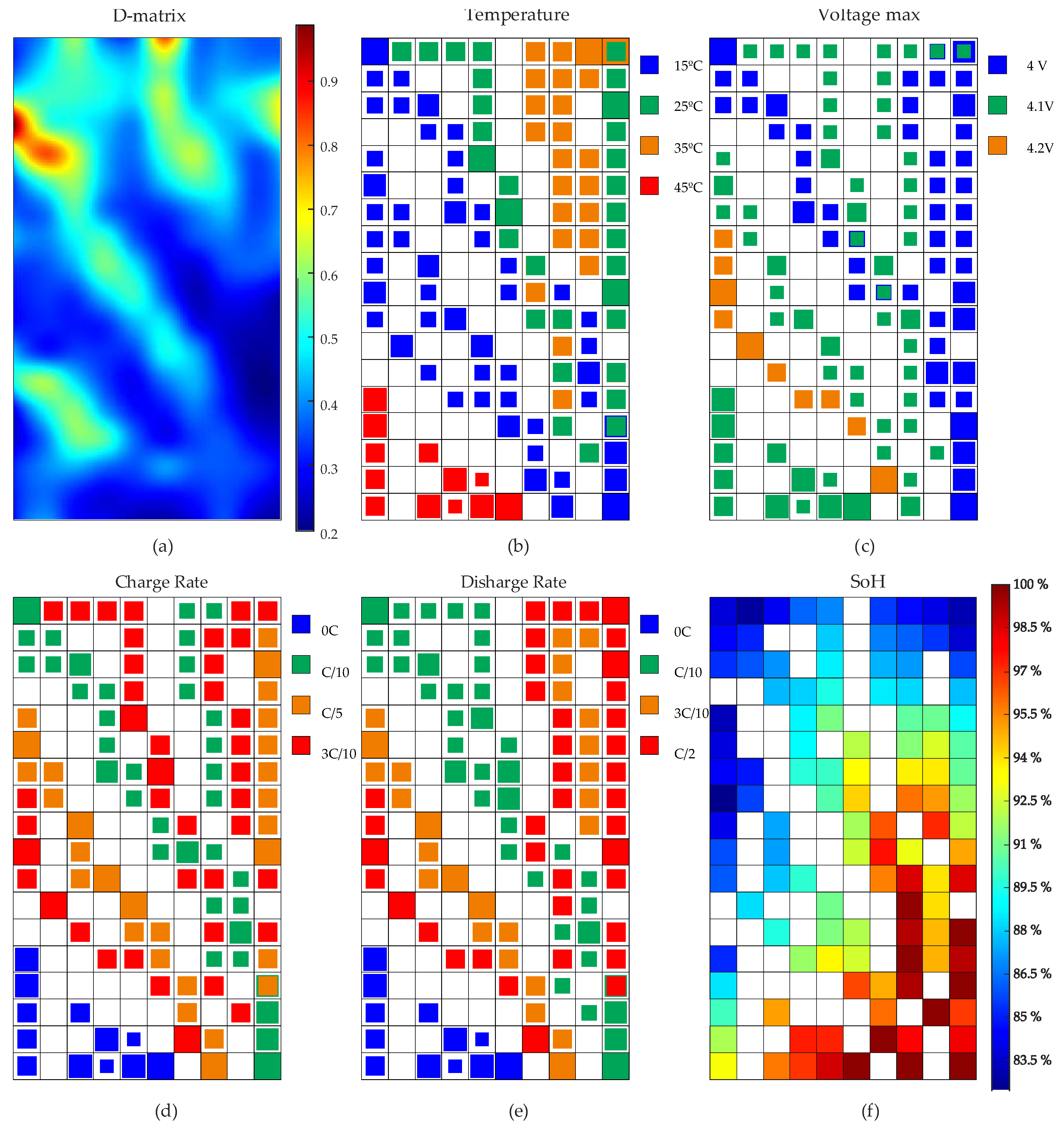
An automotive OEM has provided the database used in this work; neither cell references nor manufacturer can be revealed for confidentiality reasons. The dataset consists of thirteen NCA (LiNiCoAlO₂) 18,650 Li-ion cells with a nominal voltage and capacity of 3.6 V and 3.2 Ah, respectively.

Cells were continuously cycled in environmental chambers simulating real conditions of usage with a different profile for each cell (different Vmax, charge/discharge rates, temperatures, etc.), thus, each cell suffered different degradation processes depending on each specific application (described in

Table 1. Cycling conditions during normal operation for each cell of the study.

Name	Vmax [V]	Charge Rate [[–]	Discharge Rate [[–]	Room Temp [°C]	End of Life [%]	Number of Control Tests
1	4.1	-	-	25	93	42
2	4.1	-	-	35	90	41
3	4.1	-	-	45	74	35
4	4.1	-	-	60	90	20
5	4	$\raisebox{1ex}{$\mathrm{C}$}\!\left/ \!\raisebox{-1ex}{$10$}\right.$	$\raisebox{1ex}{$\mathrm{C}$}\!\left/ \!\raisebox{-1ex}{$10$}\right.$	15	76	42
6	4.1	$\raisebox{1ex}{$\mathrm{C}$}\!\left/ \!\raisebox{-1ex}{$5$}\right.$	$3\raisebox{1ex}{$\mathrm{C}$}\!\left/ \!\raisebox{-1ex}{$10$}\right.$	15	70	42
7	4.2	$3\raisebox{1ex}{$\mathrm{C}$}\!\left/ \!\raisebox{-1ex}{$10$}\right.$	$\raisebox{1ex}{$\mathrm{C}$}\!\left/ \!\raisebox{-1ex}{$2$}\right.$	15	80	19
8	4	$\raisebox{1ex}{$\mathrm{C}$}\!\left/ \!\raisebox{-1ex}{$5$}\right.$	$\raisebox{1ex}{$\mathrm{C}$}\!\left/ \!\raisebox{-1ex}{$2$}\right.$	25	66	37
9	4.1	$3\raisebox{1ex}{$\mathrm{C}$}\!\left/ \!\raisebox{-1ex}{$10$}\right.$	$\raisebox{1ex}{$\mathrm{C}$}\!\left/ \!\raisebox{-1ex}{$10$}\right.$	25	65	37
10	4.2	$\raisebox{1ex}{$\mathrm{C}$}\!\left/ \!\raisebox{-1ex}{$10$}\right.$	$3\raisebox{1ex}{$\mathrm{C}$}\!\left/ \!\raisebox{-1ex}{$10$}\right.$	25	92	19
11	4	$3\raisebox{1ex}{$\mathrm{C}$}\!\left/ \!\raisebox{-1ex}{$10$}\right.$	$3\raisebox{1ex}{$\mathrm{C}$}\!\left/ \!\raisebox{-1ex}{$10$}\right.$	35	80	19
12	4.1	$\raisebox{1ex}{$\mathrm{C}$}\!\left/ \!\raisebox{-1ex}{$10$}\right.$	$\raisebox{1ex}{$\mathrm{C}$}\!\left/ \!\raisebox{-1ex}{$2$}\right.$	35	85	19
13	4.2	$\raisebox{1ex}{$\mathrm{C}$}\!\left/ \!\raisebox{-1ex}{$5$}\right.$	$\raisebox{1ex}{$\mathrm{C}$}\!\left/ \!\raisebox{-1ex}{$10$}\right.$	35	85	19

* Vmin for all the applications was 2.9 V. Charge and discharge rates based on the C-rate (if nominal capacity was 1 Ah, 1 A current would be 1 C).

). Homogeneous control tests were carried out periodically for all the cells. This dataset was formed by control tests carried out for almost four years. The control tests have a sampling frequency of 1 Hz.

The database does not include information corresponding to the continuous real application–simulation cycles. There is only information from the homogeneous tests (charge and discharge) that were performed periodically to all cells to check their status.

This database is useful for degradation studies, since it includes data from homogeneous tests from cells being used in diverse conditions of use, different applications (in operation or stored), temperature conditions, and current rates as well as maximum charging voltage. Notice that several cells did not reach their End of Life (EoL) point. Since this database was provided by an external party, there was no information about the design of experiment (DoE) about this term.

Although it has similarities with other databases that are widely used for degradation studies, such as the one provided by NASA [34], these other databases do not include information on the cycles themselves, and no similar tests for all cells are included.

Cycling conditions during normal operation for each cell can be consulted in Table 1. The first four cells were simply stored (unused) between experiments at high voltage and constant temperatures; the rest of the cells were cycled with different conditions and a constant-current profile.

Control tests were performed on the 13 cells, however, within the course of the experiment, some cells reached their EoL. In total, 42 stops from the normal cycling conditions were made to carry out control tests. These tests were made approximately every 6 weeks during the 4 years that the experiment lasted. Some cells reached their End of Life early, and a lower number of tests could be performed (Table 1 shows the number of tests carried out for every cell). Thus, in total, 391 control tests were made.

The control tests consisted of a full constant-current, constant-voltage (CC/CV) charge/discharge profile with a current rate of C/3, from 4.1 V to 3 V, and a cut-off current of 65 mA at a constant ambient temperature of 25 °C.

The normalized control tests (dataset) analyzed in this article can be consulted in [35].

2.3. Preprocessing and Feature Extraction

The aim of our work consists of developing a methodology for cell aging estimation (Figure 2) complementary to the classical definition of SoH, where only battery capacity is considered. For this reason, in our work the discharge curve is converted to a normalized form. This removes all information on the cell capacity, which is related to the maximum charged or discharged capacity at each moment of its life cycle.

The State of Health (SoH) values were calculated with the capacity fade approach [14]:

$$SoH(t)=\frac{Q_{max}(t)}{Q_{nominal}}\cdot 100\begin{array}{cc}& [\%]\end{array}$$

(6)

where Q_max(t) represents the maximum capacity discharged on each of the control tests (calculated with Coulomb Counting), and Q_nominal represents the initial capacity of each cell when manufactured.

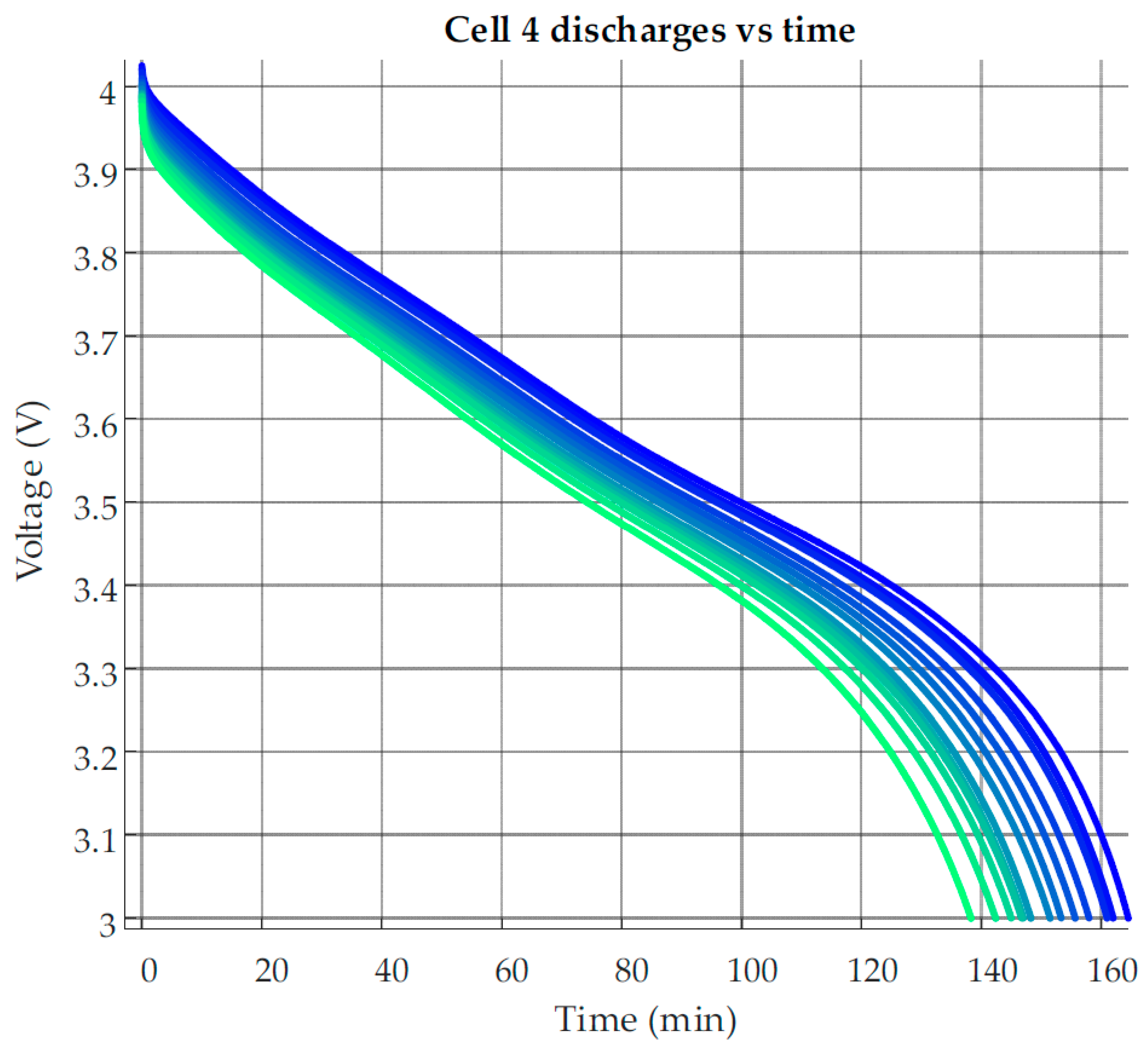
EoL points are very different from each discharge curve of the dataset (Figure 4). It was decided to study the available aging data up to the 85% SoH level (Figure 5). Our goal was to check if a SOM can differentiate causes of aging from discharge data recorded in similar degradation conditions. The duration of the discharge (Figure 6), i.e., the length of the curve on the x-axis, depends on the product of the capacity and the discharge current. The capacity information must be removed to validate the study hypothesis. Therefore, to ensure that the discharge curve of the voltage does not depend on the cell capacity, it has been normalized using the state of charge (SoC), as defined in Equation (7), as it is a relative magnitude.

$$SoC(t)=100\cdot \left(1-\frac{Q_{discharged}(t)}{Q_{max}(cycle)}\right)\begin{array}{cc}& [\%]\end{array}$$

(7)

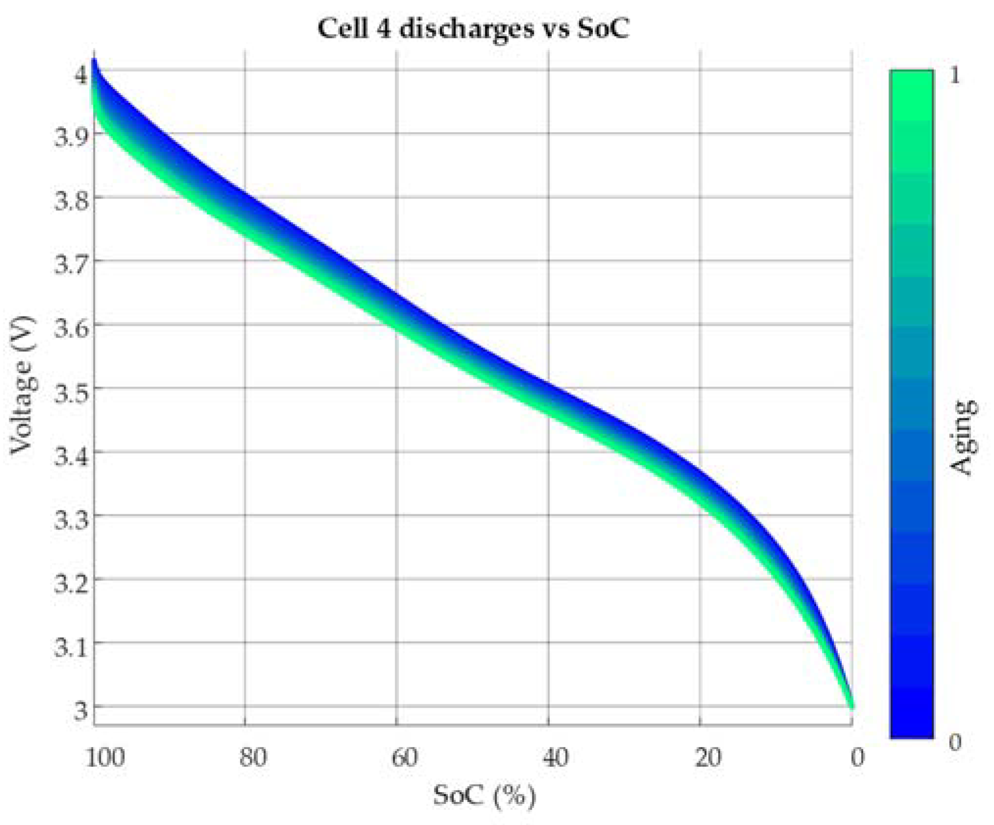
Voltage-SoC curves were obtained from the discharge part of the control tests, using Coulomb Counting. For each cycle, the maximum discharged capacity was considered 100% SoC, as can be observed in Figure 7.

Some studies, such as [36], propose differential features between several cycles, but these techniques require several laboratory cycles, reducing their useful life in real applications. Others study the degradation only with the capacity feature [37], but as explained in the introduction, two cells can have the same capacity at a certain point in their life cycle but can have a totally different aging curve. Other approaches extract statistical features, such as the kurtosis or the skewness of the curve [38].

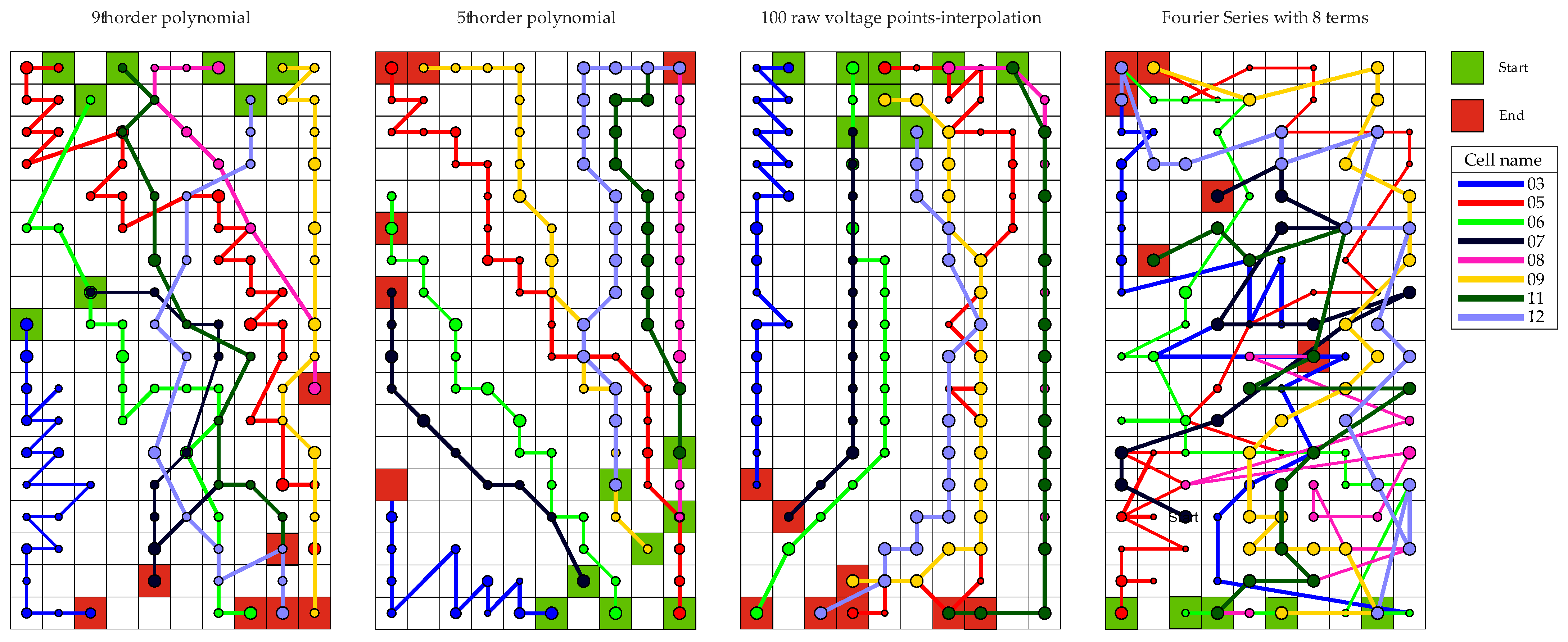
In our work, three ways of presenting the input data (input vectors) for training the SOM were tried. First, the waveforms from voltage-SoC curves were interpolated to achieve curves with 10 points, 20 points, 50 points and 100 points to be used as input vectors.

On the other hand, as is usual in machine learning, several feature extraction techniques were tried (Stage 2 in Figure 2). Thus, some statistics (mean, median, average absolute deviation, kurtosis and skewness of the curves) were used as input features.

In addition, various mathematical expressions have been proposed to fit the normalized discharge curves (mean 0, standard deviation 1), and their fitting parameters (coefficients) will be the SOM input features. The mathematical expressions tried were (

Table 2. Functions f(x) selected to fit the discharge voltage curve, with their representation errors and number of coefficients required.

Expression	Mean SSE [V2]	Mean RMSE [V]	Number of Coefficients
$f(x)=a_0+{\displaystyle \sum _{i=1}^5(a_i\cos (i\cdot x\cdot w)+b_i\sin (i\cdot x\cdot w))}$	3.98 × 10−4	2.1 × 10−3	12
$f(x)=a_0+{\displaystyle \sum _{i=1}^8(a_i\cos (i\cdot x\cdot w)+b_i\sin (i\cdot x\cdot w))}$	4.88 × 10−5	7.39 × 10−4	18
$f(x)={\displaystyle \sum _{i=1}^4{a}_i{e}^{-{\left(\frac{x-b_i}{c_i}\right)}^2}}$	9.38 × 10−4	3.10 × 10−3	12
$f(x)={\displaystyle \sum _{i=0}^5{a}_i{x}^i}$	1.70 × 10−3	4.10 × 10−3	6
$f(x)={\displaystyle \sum _{i=0}^9{a}_i{x}^i}$	4.70 × 10−4	2.20 × 10−3	10
$f(x)=\frac{a_{1}x}{{\displaystyle \sum _{i=0}^4{b}_i{x}^i}}$	4.10 × 10−3	6.30 × 10−3	6

* f(x) models the output voltage; x represents the input SoC point; a_i, b_i, c_i and w are the fitting parameters.

) Fourier series (5 and 8 terms), Gaussian model (4 terms), 5th- and 9th-degree polynomials and rational fraction. The goodness-of-fit was checked by using the average root-mean-square error (RMSE) and the sum of squared errors (SSE) as metrics.

The results achieved by using all these techniques will be shown in Section 3.

2.4. Metrics

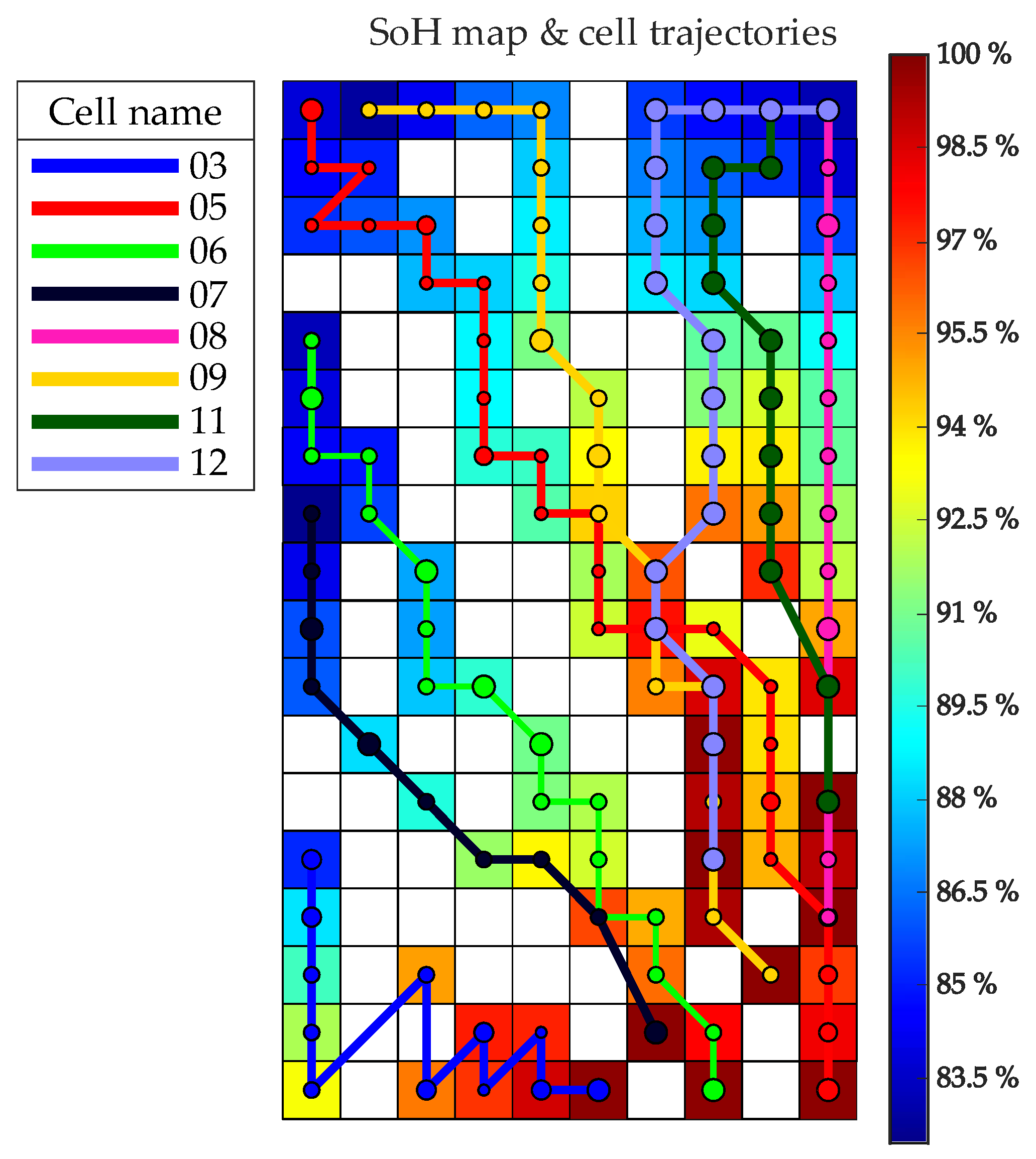
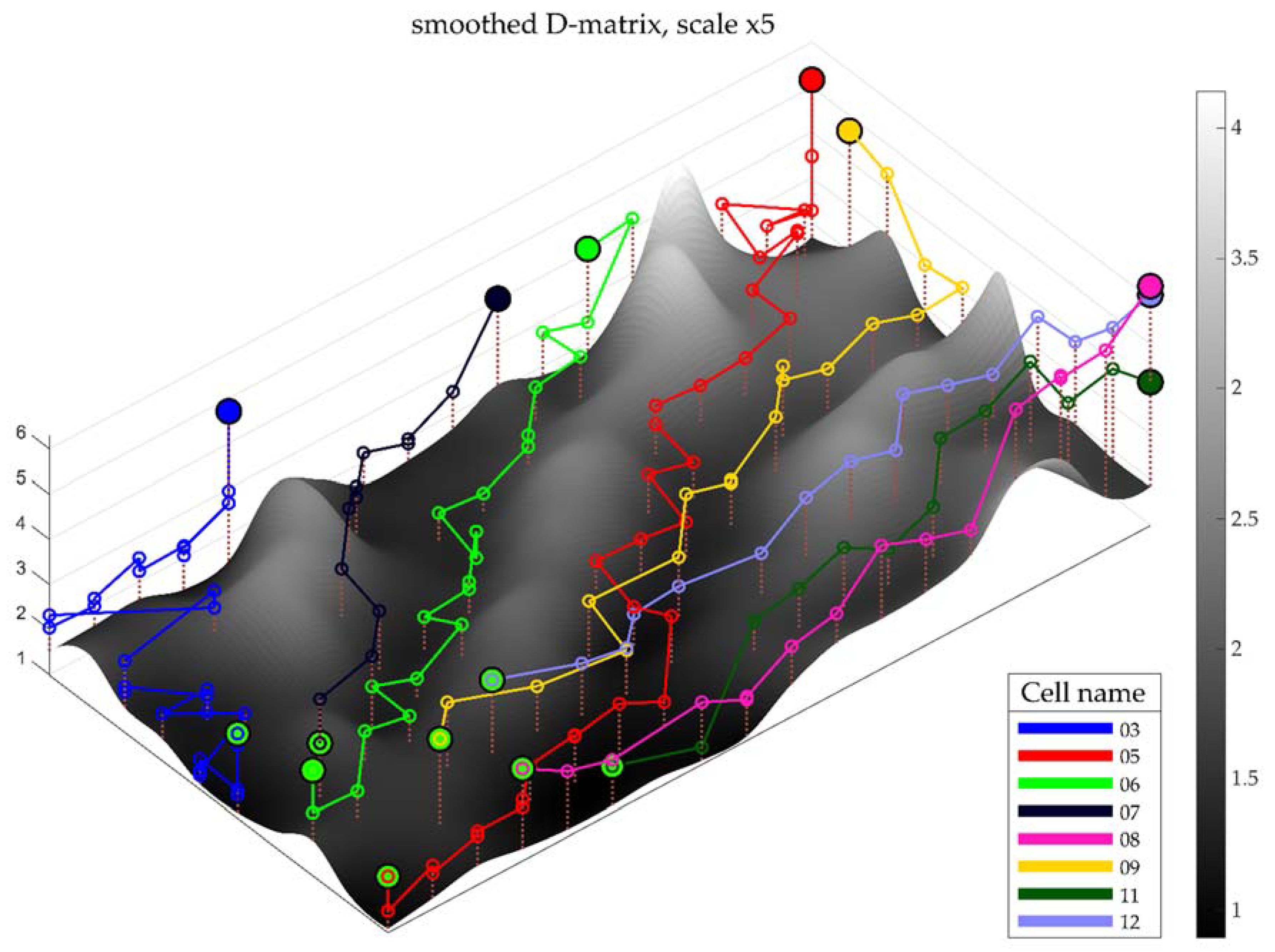
Usually the results provided by the SOM are visual and qualitative [31,32]; metrics such as quantization error and topological error (Section 2.1) only inform about the quality of the trained map. Once trained, the map is used for representing the evolution of the aging of a battery cell in the form of a trajectory or path of BMUs (Figure 8 and Figure 9). Here, two new metrics were introduced to evaluate and compare cell trajectories on the map because no SOM quality criteria applied to the evaluation of trajectories was found in the literature.

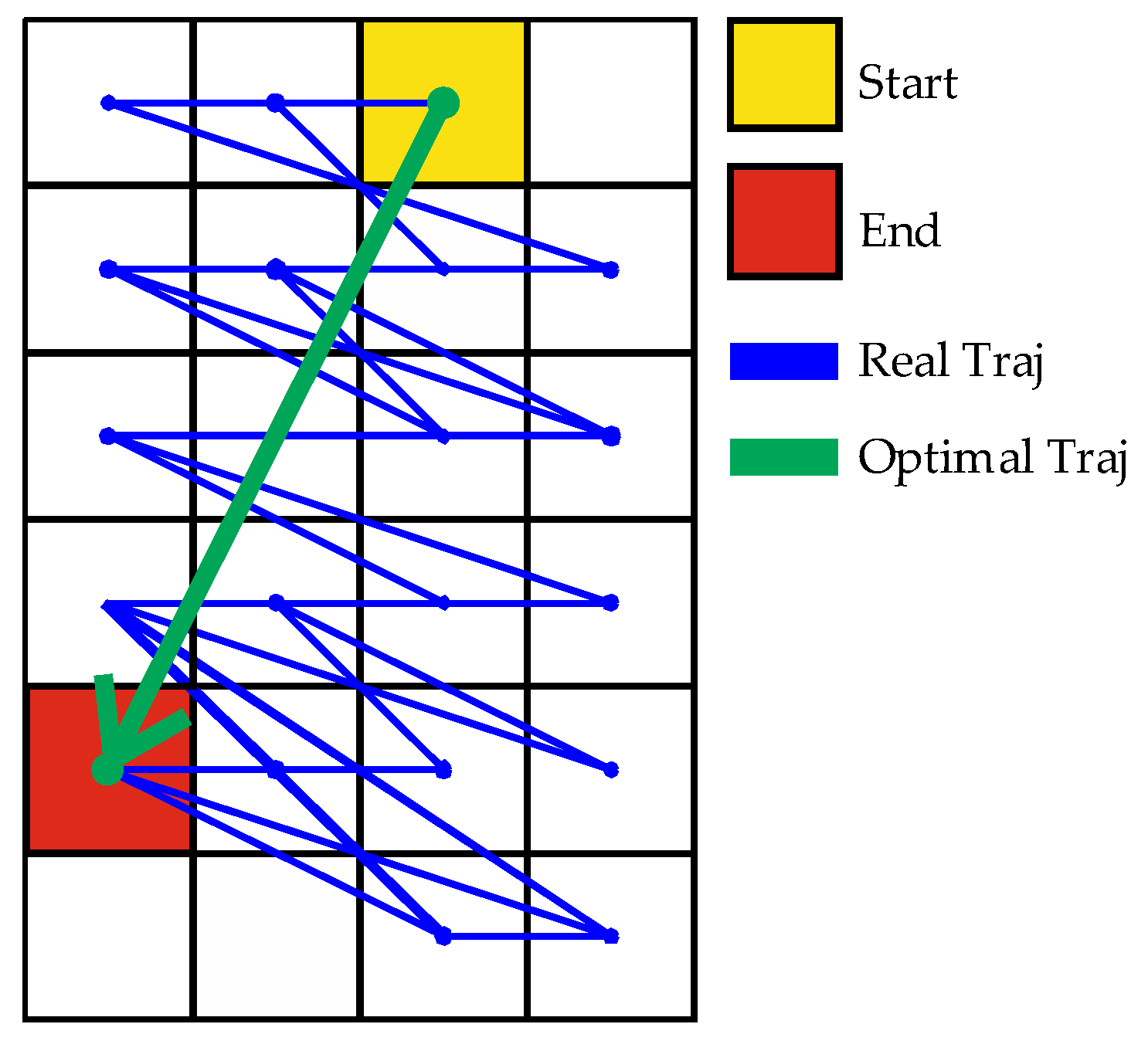
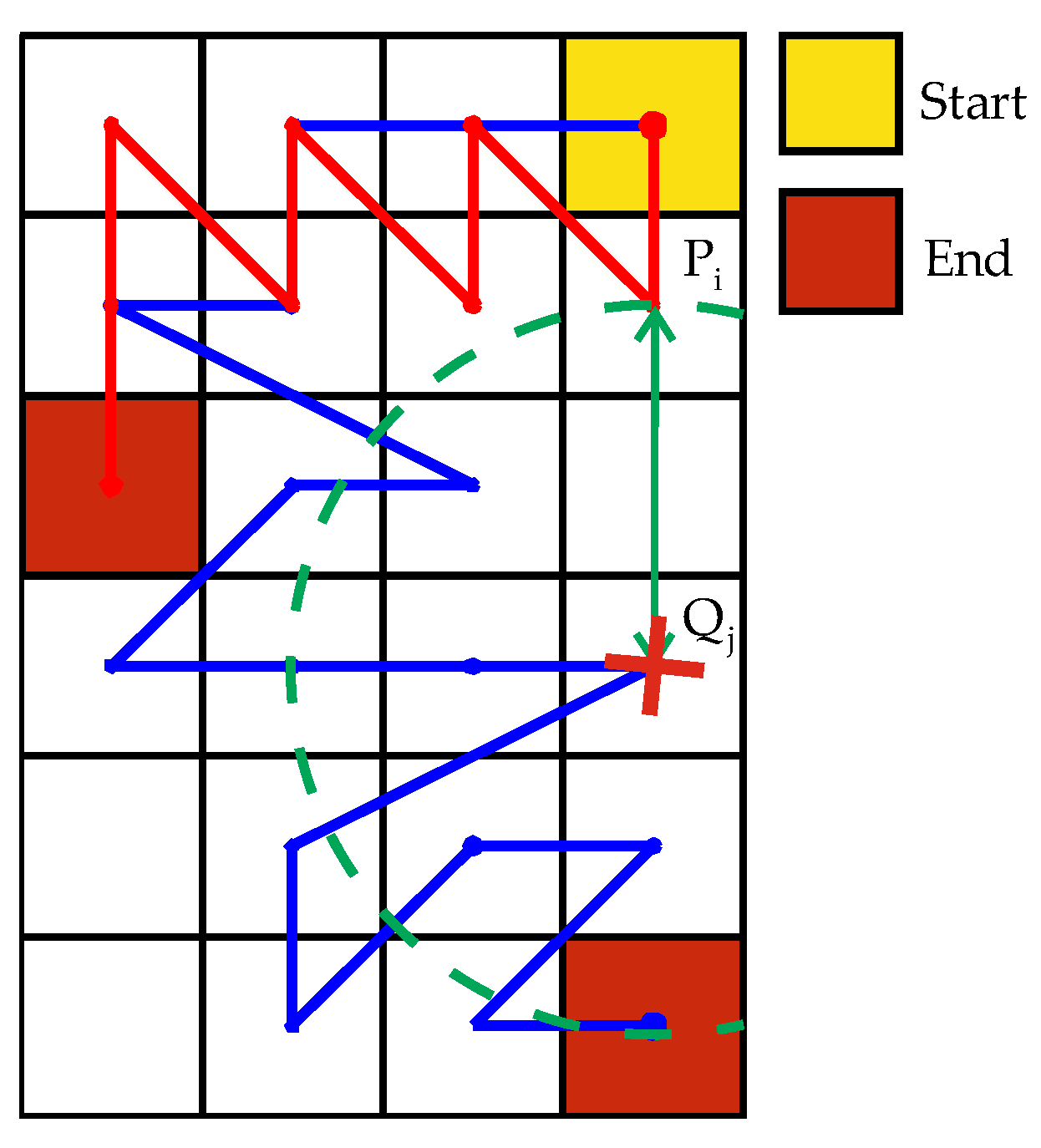
The first proposed metric, the relative deployment index (DI), assesses the quality of the trajectory deployment. It is desirable that a trajectory on the map has a length as close as possible to the minimum distance between the initial and the final point (Figure 8). Thus, first, the length of a specific trajectory is calculated and then divided by the minimum possible length: Given a trajectory of N points, its length is evaluated by adding the Manhattan distances [39] between all its consecutive points P_i and P_i−1, and then it is divided by the Euclidean distance (d_E) between the start (P₁) and end (P_N) points:

$$DI=\frac{{\displaystyle \sum _{i=2}^N\left|P_i-P_{i-1}\right|}}{d_E(P_N,P_1)}=\frac{{\displaystyle \sum _{i=2}^N\left(\left|P{x}_i-P{x}_{i-1}\right|+\left|P{y}_i-P{y}_{i-1}\right|\right)}}{\sqrt{{(P{x}_N-P{x}_1)}^2+{(P{y}_N-P{y}_1)}^2}}$$

(8)

where, given a point P, Px and Py represent its x and y coordinates on the map. Thus, a trajectory with DI close to the unit indicates a good trajectory (close to optimal, Figure 8).

The second proposed metric, separability index (SI), compares several trajectories (on the same map) against each other to assess their separability (similarity). SI measures the geometric distance between two trajectories on the map (related to their size); similar trajectories will have a low SI.

This metric computes the deployment distances between two trajectories. For each point in one trajectory Q_j (marked as X in red in Figure 9), the minimal distance to the other trajectory P_i (for all the points i) is calculated on a radial base, selecting the value of the (minimum) distance, represented with green dots in Figure 9.

As distances are calculated on a squared grid, the Manhattan distance was selected in order to consider all the adjacent neurons at the same distance

$$SI=\frac{{\displaystyle \sum _{i=1}^N\underset{j}{\min }\left|P_i-Q_j\right|}}{{\displaystyle \sum _{i=2}^N\left|P_i-P_{i-1}\right|}}$$

(9)

The numerator adds the minimum Manhattan distances calculated between all the points of the first trajectory, P_i, with each of the points of the other trajectory, Q_j. To normalize this measure, it is divided by the length of the trajectory, with the aim of relativizing this distance regardless of the dimension of the map or of the trajectories studied. Thus, cases with equally separated trajectories but different lengths will produce different SI. The calculations of this separability index for pairs of trajectories are presented in a matrix form (as in a confusion matrix), to quantify the relative unfolding between all possible combinations of trajectories on a map trained with several battery cells.

For measuring the deployment quality of the trajectories, the number of coincident BMUs (NoCB), based on the Hamming distance [40], was proposed.

This metric measures the minimum number of required changes between two series so one can become the other. Then, the NoCB represents the maximum number of BMUs from a trajectory map, which are coincident to another trajectory. A high NoCB means that the corresponding two cell cycles are interpreted by the SOM as equals.

3. Results

3.1. Discharge Maps

This section shows the results achieved by our three-step methodology (Figure 2) by incorporating the tools shown in Section 2. In the first step, the voltage-time curve is normalized to the voltage-SoC curve to remove the information on cell capacity (as explained in Section 2.3). The second step, feature extraction, depends on the specific feature extraction technique selected of those presented in Section 2.3. In the third step, the data are introduced as inputs to the SOM, the map is trained and, finally, metrics are calculated, and the results are analyzed.

The SOM allows for displaying information in different ways [31,32]; for this work, labeled maps, feature maps, trajectory maps and 3D visualizations are shown and discussed.

From the initial 391 control tests, 165 were made of cells with a SoH metric above 85% (eight cells in total, selected as explained in Section 2.3). SOMs were trained with 165 input vectors (examples) from those 165 control tests. An input vector consists of data of a battery cycle, including the features extracted from discharge curves or raw discharge data (Section 2.3).

The SOM Toolbox library [41] was used for developing the maps. This library automatically sets the hyperparameters, nevertheless, the SOM is usually very tolerant to the specific value of many of its hyperparameters. The main hyperparameter is the dimension of the map (nx × ny neurons, Section 2.1). In most SOM applications, the number of neurons on the map should be similar to the number of training examples (165 control tests in our case), in order to get the input data to be well separated onto the map when projected. In our case, we used 10 × 18 maps (Figure 10), i.e., 180 neurons, because it is a number close to the 165 training samples available. In its operation, the SOM distributed the 165 training samples among the 180 neurons and the training samples projected to the map were well separated (one sample per neuron, approximately).

Table 3. Metrics for 10 × 18 SOMs trained with input data obtained by using different feature extraction techniques.

Input Features	qe	te	Mean SI	Max SI	Mean DI	Max DI	Mean NoCB	Max NoCB
Statistics	0.31	0.11	2.05	13.20	1.28	1.72	0.31	11
Raw Voltage 10 points	0.45	0.11	0.48	2.76	2.83	4.08	0.75	7
Raw Voltage 20 points	0.56	0.10	0.75	3.75	2.05	3.30	0.70	7
Raw Voltage 50 points	0.77	0.15	0.96	4.87	1.62	2.63	0.63	8
Raw Voltage 100 points	0.02	0.15	1.24	6.63	1.34	1.84	0.48	11
Fourier Series, with 5 terms	0.02	0.22	0.25	1.17	10.56	18.23	6.70	65
Fourier Series with 8 terms	0.12	0.15	0.47	2.02	2.89	4.66	0.59	6
Gaussian Model with 4 terms	0.36	0.05	0.30	1.42	5.48	9.72	0.48	4
5th Degree Polynomial	0.22	0.15	2.23	12.46	1.36	2.29	0.20	3
9th Degree Polynomial	0.22	0.05	1.37	9.80	1.61	2.33	0.33	4
Rational fraction	0.10	0.27	0.22	1.08	9.87	16.09	1.03	17

shows the achieved results for 10 × 18 SOMs trained by using the different feature extraction techniques explained in Section 2.3. The first two metrics, quantization (q_e) and topographic error (t_e), measure the quality of the trained map, as explained in Section 2.1. The other shown values are the maximum and mean deployment index (DI) and separability index (SI), and the number of coincident BMUs (NoCB), as defined in Section 2.4. For q_e, t_e, DI and NoCB, the lower the value, the better. In the case of the SI, a higher value indicates a greater distance between trajectories (better separability).

It can be observed in Table 3 that satisfactory values for quantization and topographic errors are achieved in all cases. The best SI is obtained by using as inputs sample statistics and the coefficients of 5th degree polynomials. In the case of the deployment index, the best results are obtained with sample statistics, interpolated voltages (100 points) and the 5th degree polynomial. Finally, the lowest NoCB are found when using 5th degree polynomials, both in average and maximum values.

In Figure 10, some maps trained by using several feature extraction techniques were included to show the deployment quality of eight cell trajectories. Notice that, once trained, the SOM is used in inference: An input vector (cell cycle) is presented, every neuron computes Equation (1) and the winning neuron (BMU) is marked. Presenting a series of input vectors corresponding to the cycles of a specific cell, its evolution is displayed as an aging trajectory that links all the BMUs. Best results are given by raw voltages (100 points) and the 5th order polynomial.

Given the quantitative results (Table 3) and the visual analysis of the deployed trajectories (Figure 10), feature extraction based on modeling the voltage-SoC curve by using a 5th degree polynomial is a good choice:

$$V(x)=a_5\cdot x^5+a_4\cdot x^4+a_3\cdot x^3+a_2\cdot x^2+a_1\cdot x+a_0$$

(10)

where x represents the SoC. This is the feature extraction technique shown in Figure 2.

Thus, in our methodology, normalized discharge curves (mean 0, standard deviation 1) are fitted to this 5th degree polynomial, and their six fitting parameters (a_i) are the SOM input features. From now on, only maps trained by using this feature extraction technique will be considered.

3.2. Labeled Maps

Once the SOM has been trained, in our case, by using 165 input vectors including six features (the six coefficients of a 5th degree polynomial), some visualizations can be generated (Figure 11). In Figure 11a, the D-matrix of the trained SOM is shown, representing a map of mean distances between neighboring neurons (as explained in Section 2.1).

The bigger the distance (yellow and red colors), the bigger the difference between the information learned by the neighboring neurons, which allows delimiting natural borders on the map (possible clusters). Blue valleys (similar neurons) are separated by yellow and red boundaries (frontiers), separating input vectors with very different features. Thus, D-matrix in Figure 11a helps to interpret clusters shown in the following analysis involving labels, features and trajectories.

For the other map visualizations, all the input vectors used for training (corresponding to the cell cycles under analysis) are presented to the SOM. The BMU corresponding to every cell cycle is colored in relation to the following labels (Figure 11): temperature (15 °C, 25 °C, 35 °C, 45 °C), charging current (0, C/10, C/5, 3C/10), discharging current (0, C10, 3C/10, C/2), maximum operating voltage (4 V, 4.1 V, 4.2 V) and SoH status of each cycle (some values between 80% and 100%). For instance, in the temperature map of Figure 11b, 15 °C is represented in blue, 25 °C in green, 35 °C in orange and 45 °C in red. Lower temperatures can be found in the center of the map, whereas higher ones are on the map extremes (35 °C on the right part of the map and 45 °C on the lower part).

In the case of the maximum voltage (Figure 11c), lower voltages are found in the upper right zone of the map, whereas higher voltages are at the lower left of the map.

Figure 11d,e show the labels corresponding to the charge and discharge rate, respectively. In both maps there is a zone at the bottom corresponding to the cell that was stored without being charged. On the other hand, in Figure 11e a central cluster can be distinguished for cells discharged at a current rate of C/10, but there are no separate clusters for cells with current rates of C/2 and 3C/10.

Figure 11f shows the SoH corresponding to each of the cycles used for training. A clear progression can be observed, from the lower right area (red), where all the new cell cycles are found, towards the rest of the map, where aging is increasing. This disposition seems coherent since the impact of the different conditions of use in new cells is less determinant in their voltage responses. As they degrade, differences are observed, just as they would be seen in their equivalent electrical models.

Finally, as an illustration of the use of labeled maps, Figure 12 merges the second map of Figure 10 (trajectories of eight cells) and Figure 11f (neurons colored according to their SoH). Thus, in Figure 12 the history (aging) of eight battery cells can be appreciated: All the cell trajectories start at the lower right corner of the map (high SoH) and end at the upper areas (low SoH). Depending on the use conditions of every battery cell, their aging diseases are different, being represented on different zones of the map.

3.3. Trajectory Maps

As already seen, by presenting to a trained SOM a series of input vectors corresponding to several cycles of a specific battery cell, the SOM provides a BMU for every input vector (cell cycle), and the evolution of that cell can be seen as an aging trajectory that links all the BMUs. The BMU is the neuron whose value provided by Equation (1) is minimum, but, in addition, this equation provides the quantization error of the input data versus the winning neuron. This error gives an idea of the confidence of the position estimation of the input vector onto the map: A low error provides confidence, while a high error suggests that the current input vector does not actually have a good match.

The new visualization of Figure 13 (3-D visualization or ‘geographic metaphor’) was developed from the D-matrix and represents the change in the weights of neighboring neurons in grey levels on the z-axis. Areas of similar weights (valleys) have low values (black color), while the areas with the greatest change in weights (white) suggest cluster borders (mountains). The cell paths and their quantization errors (represented by the height of a point over the surface) were included in the ‘geographic metaphor’ for observing the cell evolutions.

It can be seen that all the cells have their starting point (green points) in the same area of the map, with high SoH (see Figure 12). From there, each one evolves through different zones, as already seen in the labeled maps. Cells 6 and 7, with a cycling temperature of 15 °C, are located in the same valley. Cells 5 and 9, with a charging current of C/10, are located in the central valley, and cells 8, 11 and 12, with cycling temperatures of 25 °C and 35 °C, are grouped in the right zone.

In addition to visual inspection, the correct deployment of the paths can be assessed by the relative deployment index (

Table 4. Values for the relative deployment index (DI), as defined in Equation (5), for the cells under study.

Cell	3	5	6	7	8	9	11	12
DI	2.29	1.24	1.33	1.09	1.04	1.23	1.11	1.29

) and the separability index (

Table 5. Separability index (SI) as defined in Equation (6). Better results shown in green.

Cell	3	5	6	7	8	9	11	12
3	0.00	8.38	4.92	3.46	10.79	7.71	11.61	7.63
5	10.83	0.00	3.69	6.46	7.12	2.47	6.24	4.85
6	4.86	2.60	0.00	1.84	7.04	3.15	6.59	3.94
7	2.73	3.81	1.45	0.00	7.71	4.25	7.22	4.44
8	12.47	4.43	8.13	9.90	0.00	4.57	1.46	3.12
9	8.28	1.53	3.21	5.05	4.31	0.00	3.26	1.61
11	10.84	3.55	6.44	8.03	1.31	2.95	0.00	1.44
12	9.15	2.72	4.63	6.31	2.67	1.55	1.63	0.00

). The worst separability values were obtained for cells 11 and 12, as well as 9 and 12, as they are in the same area of the map. In the case of the separability index, the worst score was for cell 3, as it travels a shorter distance on the map, with a more erratic deployment.

4. Application Examples

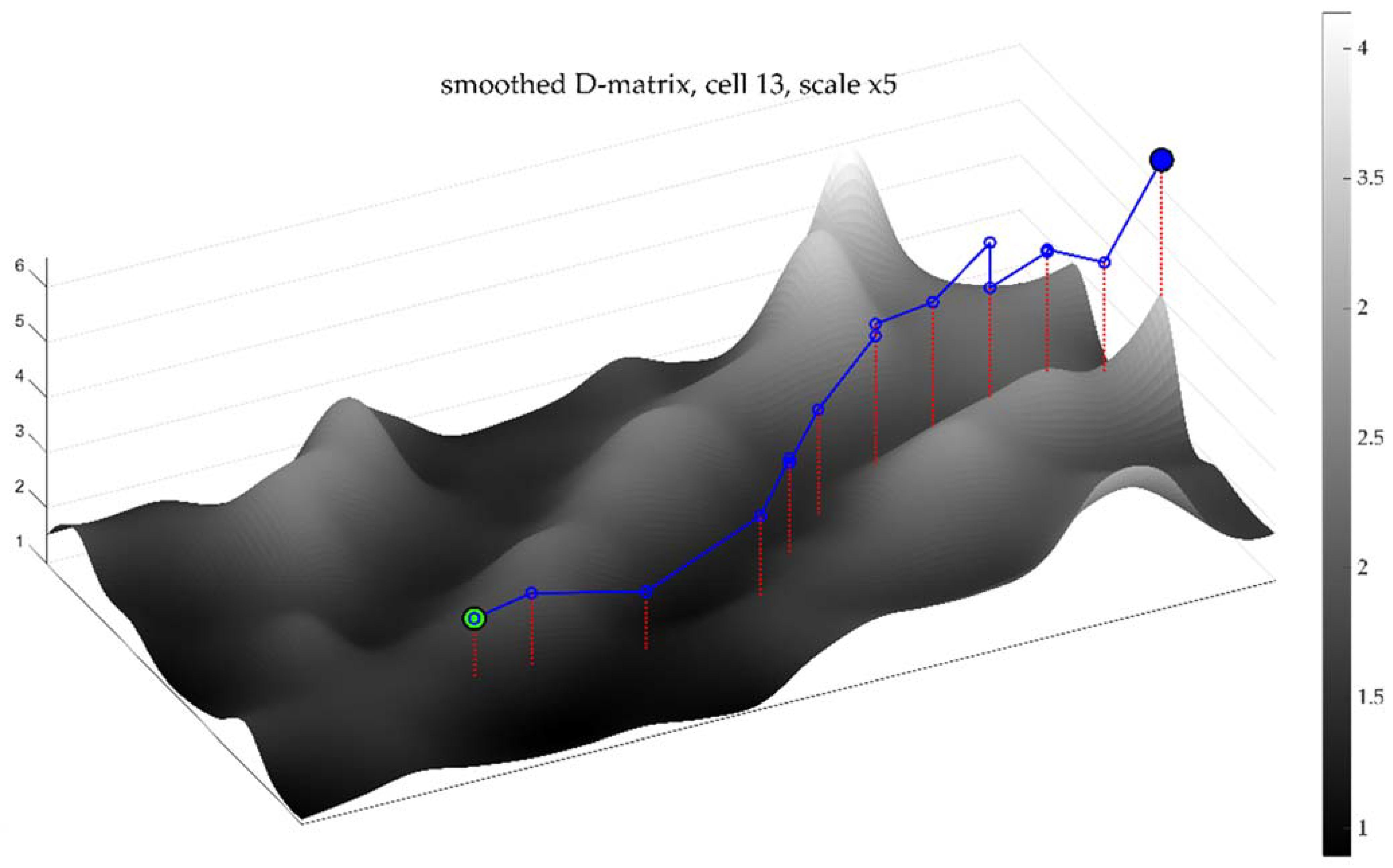
In this section, some applications of the proposed methodology are discussed. A neural network trained with a dataset can be used in inference mode, providing a response to a new input vector. For example, given a used battery destined for the second-life market, it can be analyzed (cycled) in the laboratory and the achieved data (six features in our case) can be presented to the SOM, and the BMU obtained can be used to predict is evolution.

The first application of our methodology considers a new cell, periodically extracted from its use conditions to cycle it on specific laboratory conditions and track its aging by following its evolution on the trained SOM. Cell 13, which was not included in the training dataset, was selected as an illustration. All its available input vectors (cycles) were preprocessed and applied to the trained SOM. As shown in Table 1, this cell was cycled with a room temperature of 35 °C, with a charge rate of $\raisebox{1ex}{$C$}\!\left/ \!\raisebox{-1ex}{$5$}\right.$ and discharge of $\raisebox{1ex}{$C$}\!\left/ \!\raisebox{-1ex}{$10$}\right.$.

Figure 14 shows its trajectory onto the SOM, which was deployed on the middle cluster. The distance to the map on the z-axis represents the quantization error, a measure of the certainty of the estimations that the SOM provides. A slightly bigger amount of quantization error (mean of 0.809, still a low value) in relation to the cells in Figure 13 (mean of 0.650) is due to the lack of similar data on the training dataset (the error grows with the cell aging).

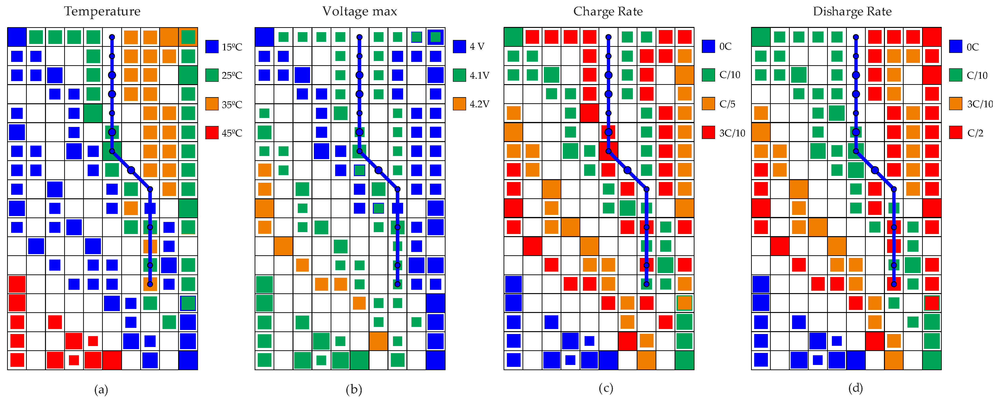
The evolution of cell 13 in relation to the label maps developed in Section 3.2 can be seen in Figure 15. The SOM processes every new input vector and provides new BMUs; notice that while some are colored BMUs, others are white BMUs (interpolating neurons).

As this cell was not included in the training dataset, some of its input vectors were more similar to interpolating neurons than to the data used for training. This means that the SOM has generalized from the training set and provides a reasonable response to new input data.

Its trajectory was on the 25 °C–35 °C valley, and it was possible to infer from Figure 15b that the cell had a similar response to the cells cycled with a maximum voltage of 4.1 V. Figure 15c,d locate the trajectory on the zone of cells cycled with a charge rate between C/10 and 3C/10 and discharge rate between C/10 and C/2.

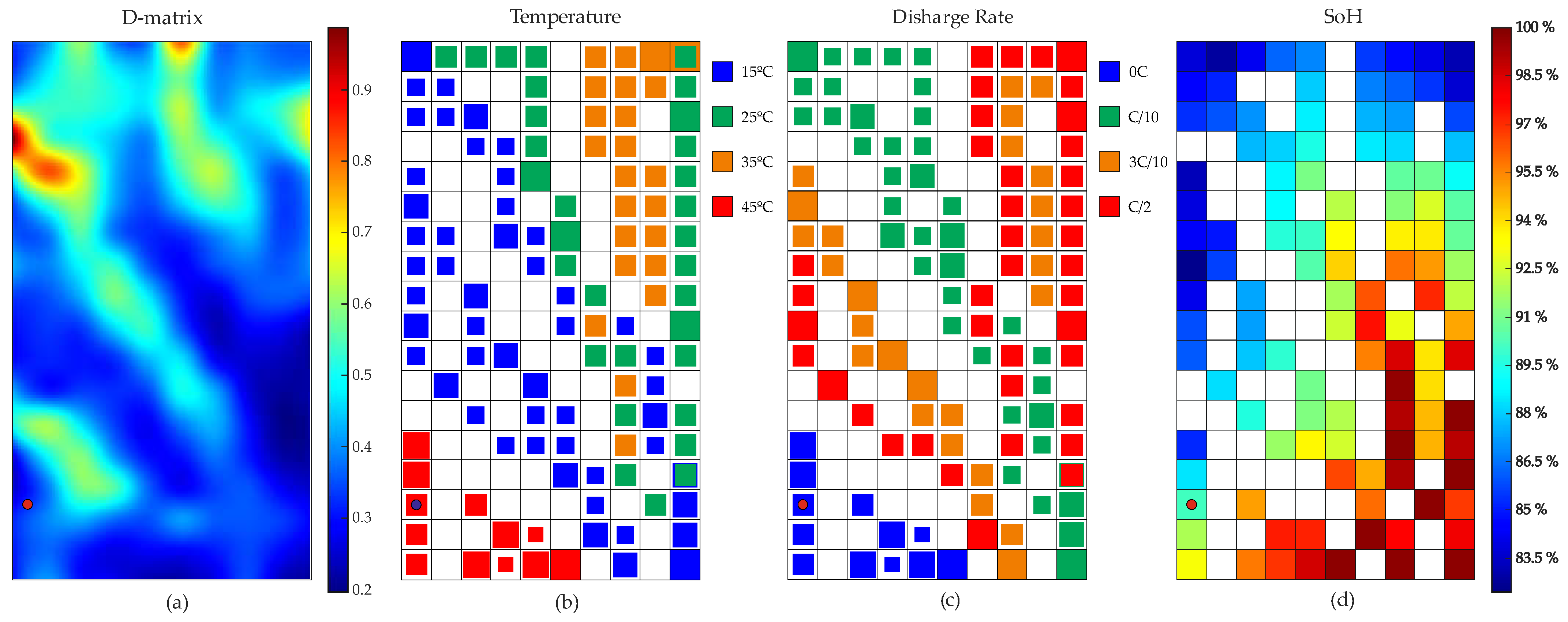
The second application shows how the proposed technique could predict the past conditions of use of a used battery. In order to evaluate a used cell, laboratory tests similar to the one carried out on the cells in the dataset must be performed. Then, these data must be preprocessed, and the resulting six features (polynomial parameters) are the SOM inputs; finally, the BMU is marked on the map.

To simulate this process, the last cycle of cell 2 (not included in the training test) was selected. This cell was stored at 35 °C and its End-of-Life was 90%. For the selected cycle, the results are shown in Figure 16 as a point on the output BMU, located on the lower left part corner of the map. As it can be seen in Figure 16b, the cycle was clustered on the 45 °C zone due to the lack of cells stored at 35 °C in the training set. Results match conditions for charge and discharge rates (as shown in Figure 16c), as the BMU is located on the zone of cells stored. The BMU represents a similar SoH condition for the presented cycle, as it is located between 90–91% of SoH. With this result, a life evolution similar to the cells located in this part of the map could be predicted.

5. Conclusions

This work proposes a new methodology that combines self-organizing maps with feature extraction based on polynomial coefficients to represent the aging of Lithium-ion cells with different usage conditions. This methodology for battery smart sensing, based on two-dimensional maps that process voltage curves, is intended to complement conventional unidimensional metrics, such as SoH, where only battery capacity is considered.

The SOM is a well-known tool for unsupervised data analysis, but in this work some new metrics were proposed to assess the unfolding of the cell trajectories, and 3D visualizations were introduced that allowed a clear view of the quantization error to determine the uncertainty of the map diagnosis.

On the one hand, all these new tools have showed that a 5th degree polynomial fitting is an appropriate feature extraction technique for this problem. On the other hand, all these new tools validate our methodology, since the trajectories of the cells on the map are separated and well defined, and the different aging phases can be located. The eight example cells used in the study are well-separated temperature-wise, being able to differentiate between high- and low-temperature applications.

In addition, as an illustration of the usefulness of our methodology, two cases of use of the trained SOMs were presented. The first one considered a new cell with periodical control tests in specific laboratory conditions, which allows tracking its aging by following its evolution on the trained SOM. The second one presented the application of this methodology to identify the state of a cell from previous unknown use in order to estimate its previous uses, actual state and predict its life expectancy depending on its state of disease, or aging. This was done by comparing with cell trajectories included in the training dataset.

Although the achieved results are promising, the dataset used in our study only includes 13 cells and in very specific situations. For a deep validation of the proposed methodology and for accurate results, a larger dataset with broader usage conditions would be required, but currently only limited databases are available.

Finally, by using maps trained with more complete databases, this technique could be used to visualize aging in batteries destined for the second-life market with unknown past uses. For instance, it would allow for assigning second-life applications that are a more adequate fit for used cells based on their capabilities.

References

1. Steward, D.; Mayyas, A.; Mann, M. Economics and challenges of Li-ion battery recycling from end-of-life vehicles. Procedia Manuf. 2019, 33, 272–279. [Google Scholar] [CrossRef]
2. Ambrose, H.; Kendall, A. Understanding the future of lithium: Part 1, resource model. J. Ind. Ecol. 2020, 24, 80–89. [Google Scholar] [CrossRef]
3. Martin, G.; Rentsch, L.; Höck, M.; Bertau, M. Lithium market research—global supply, future demand and price development. Energy Storage Mater. 2017, 6, 171–179. [Google Scholar] [CrossRef]
4. Curry, C. Lithium-Ion Battery Costs and Market Squeezed Margins Seek Technology Improvements & New Business Models. 2017. Available online: https://data.bloomberglp.com/bnef/sites/14/2017/07/BNEF-Lithium-ion-battery-costs-and-market.pdf (accessed on 11 September 2021).
5. Rallo, H.; Benveniste, G.; Gestoso, I.; Amante, B. Economic analysis of the disassembling activities to the reuse of electric vehicles Li-ion batteries. Resour. Conserv. Recycl. 2020, 159, 104785. [Google Scholar] [CrossRef]
6. Rallo, H.; Casals, L.C.; de la Torre, D.; Reinhardt, R.; Marchante, C.; Amante, B. Lithium-ion battery 2nd life used as a stationary energy storage system: Ageing and economic analysis in two real cases. J. Clean. Prod. 2020, 272, 122584. [Google Scholar] [CrossRef]
7. Casals, L.C.; Barbero, M.; Corchero, C. Reused second life batteries for aggregated demand response services. J. Clean. Prod. 2019, 212, 99–108. [Google Scholar] [CrossRef]
8. Assunção, A.; Moura, P.S.; de Almeida, A.T. Technical and economic assessment of the secondary use of repurposed electric vehicle batteries in the residential sector to support solar energy. Appl. Energy 2016, 181, 120–131. [Google Scholar] [CrossRef]
9. Bobba, S.; Mathieux, F.; Blengini, G.A. How will second-use of batteries affect stocks and flows in the EU? A model for traction Li-ion batteries. Resour. Conserv. Recycl. 2019, 145, 279–291. [Google Scholar] [CrossRef]
10. Salinas, F.; Krüger, L.; Neupert, S.; Kowal, J. A second life for li-ion cells rescued from notebook batteries. J. Energy Storage 2019, 24, 100747. [Google Scholar] [CrossRef]
11. Dubarry, M.; Qin, N.; Brooker, P. Calendar aging of commercial Li-ion cells of different chemistries—A review. Curr. Opin. Electrochem. 2018, 9, 106–113. [Google Scholar] [CrossRef]
12. Choi, S.S.; Lim, H.S. Factors that affect cycle-life and possible degradation mechanisms of a Li-ion cell based on LiCoO2. J. Power Sources 2002, 111, 130–136. [Google Scholar] [CrossRef]
13. Zhang, J.; Lee, J. A review on prognostics and health monitoring of Li-ion battery. J. Power Sources 2011, 196, 6007–6014. [Google Scholar] [CrossRef]
14. Berecibar, M.; Gandiaga, I.; Villarreal, I.; Omar, N.; van Mierlo, J.; van den Bossche, P. Critical review of state of health estimation methods of Li-ion batteries for real applications. Renew. Sustain. Energy Rev. 2016, 56, 572–587. [Google Scholar] [CrossRef]
15. Balagopal, B.; Chow, M.-Y.Y. The state of the art approaches to estimate the state of health (SOH) and state of function (SOF) of lithium Ion batteries. In Proceedings of the 2015 IEEE International Conference on Industrial Informatics, INDIN 2015, Cambridge, UK, 22–24 July 2015; pp. 1302–1307. [Google Scholar] [CrossRef]
16. Li, X.; Wang, Q.; Yang, Y.; Kang, J. Correlation between capacity loss and measurable parameters of lithium-ion batteries. Int. J. Electr. Power Energy Syst. 2019, 110, 819–826. [Google Scholar] [CrossRef]
17. Nazari, A.; Kavian, S.; Nazari, A. Lithium-Ion Batteries’ Energy Efficiency Prediction Using Physics-Based and State-of-the-Art Artificial Neural Network-Based Models. J. Energy Resour. Technol. 2020, 142, 102001. [Google Scholar] [CrossRef]
18. Tang, X.; Zou, C.; Yao, K.; Chen, G.; Liu, B.; He, Z.; Gao, F. A fast estimation algorithm for lithium-ion battery state of health. J. Power Sources 2018, 396, 453–458. [Google Scholar] [CrossRef]
19. Stroe, D.I.; Schaltz, E. Lithium-Ion Battery State-of-Health Estimation Using the Incremental Capacity Analysis Technique. IEEE Trans. Ind. Appl. 2020, 56, 678–685. [Google Scholar] [CrossRef]
20. Lipu, M.S.H.; Hannan, M.; Hussain, A.; Hoque, M.; Ker, P.J.; Saad, M.; Ayob, A. A review of state of health and remaining useful life estimation methods for lithium-ion battery in electric vehicles: Challenges and recommendations. J. Clean. Prod. 2018, 205, 115–133. [Google Scholar] [CrossRef]
21. Pastor-Fernández, C.; Yu, T.F.; Widanage, W.D.; Marco, J. Critical review of non-invasive diagnosis techniques for quantification of degradation modes in lithium-ion batteries. Renew. Sustain. Energy Rev. 2019, 109, 138–159. [Google Scholar] [CrossRef]
22. Deng, Y.; Ying, H.; E, J.; Zhu, H.; Wei, K.; Chen, J.; Zhang, F.; Liao, G. Feature parameter extraction and intelligent estimation of the State-of-Health of lithium-ion batteries. Energy 2019, 176, 91–102. [Google Scholar] [CrossRef]
23. Sanz-Gorrachategui, I.; Pastor-Flores, P.; Pajovic, M.; Wang, Y.; Orlik, P.V.; Bernal-Ruiz, C.; Bono-Nuez, A.; Artal-Sevil, J.S. Remaining Useful Life Estimation for LFP Cells in Second-Life Applications. IEEE Trans. Instrum. Meas. 2021, 70, 1–10. [Google Scholar] [CrossRef]
24. Long, B.; Li, X.; Gao, X.; Liu, Z. Prognostics Comparison of Lithium-Ion Battery Based on the Shallow and Deep Neural Networks Model. Energies 2019, 12, 3271. [Google Scholar] [CrossRef] [Green Version]
25. Zheng, Y.; Wang, J.; Qin, C.; Lu, L.; Han, X.; Ouyang, M. A novel capacity estimation method based on charging curve sections for lithium-ion batteries in electric vehicles. Energy 2019, 185, 361–371. [Google Scholar] [CrossRef]
26. Jia, J.; Liang, J.; Shi, Y.; Wen, J.; Pang, X.; Zeng, J. SOH and RUL Prediction of Lithium-Ion Batteries Based on Gaussian Process Regression with Indirect Health Indicators. Energies 2020, 13, 375. [Google Scholar] [CrossRef] [Green Version]
27. Dong, G.; Chen, Z.; Wei, J.; Ling, Q. Battery health prognosis using brownian motion modeling and particle filtering. IEEE Trans. Ind. Electron. 2018, 65, 8646–8655. [Google Scholar] [CrossRef]
28. Farhad, S.; Nazari, A. Introducing the energy efficiency map of lithium-ion batteries. Int. J. Energy Res. 2019, 43, 931–944. [Google Scholar] [CrossRef]
29. Banguero, E.; Correcher, A.; Pérez-Navarro, Á.; García, E.; Aristizabal, A. Diagnosis of a battery energy storage system based on principal component analysis. Renew. Energy 2020, 146, 2438–2449. [Google Scholar] [CrossRef]
30. Pastor-Flores, P.; Bernal-Ruiz, C.; Sanz-Gorrachategui, I.; Bono-Nuez, A.; Martin-Del-Brio, B.; Sevil, J.S.A.; Cebolla, F.J.P. Analysis of Li-ion battery degradation using self- organizing maps. In Proceedings of the IECON 2019—45th Annual Conference of the IEEE Industrial Electronics Society, Lisbon, Portugal, 14–17 October 2019; pp. 4385–4390. [Google Scholar]
31. Kohonen, T.; Oja, E.; Simula, O.; Visa, A.; Kangas, J. Engineering applications of the self-organizing map. Proc. IEEE 1996, 84, 1358–1384. [Google Scholar] [CrossRef]
32. Kohonen, T. Self-Organizing Maps, 3rd ed.; Springer: Berlin/Heidelberg, Germany, 2001. [Google Scholar]
33. Uriarte, E.A.; Mart, F.D. Topology preservation in SOM. Int. J. Appl. Math. Comput. Sci. 2005, 1, 19–22. [Google Scholar]
34. Saha, B.; Goebel, K.; Christophersen, J. Comparison of prognostic algorithms for estimating remaining useful life of batteries. Trans. Inst. Meas. Control 2009, 31, 293–308. [Google Scholar] [CrossRef]
35. Control_Tests_Aging. 2021. Available online: https://github.com/Batt-Repository/data_control_tests_aging (accessed on 30 August 2021).
36. Severson, K.A.; Attia, P.M.; Jin, N.; Perkins, N.; Jiang, B.; Yang, Z.; Chen, M.H.; Aykol, M.; Herring, P.K.; Fraggedakis, D.; et al. Data-driven prediction of battery cycle life before capacity degradation. Nat. Energy 2019, 4, 383–391. [Google Scholar] [CrossRef] [Green Version]
37. Yang, N.; Feng, J.; Sun, Q.; Liu, T.; Zhong, D. Online estimation of state-of-health for lithium ion batteries based on charge curves. In Proceedings of the 2016 11th International Conference on Reliability, Maintainability and Safety: Integrating Big Data, Improving Reliability and Serving Personalization, ICRMS 2016, Hangzhou, China, 26–28 October 2017; pp. 1–8. [Google Scholar] [CrossRef]
38. He, Z.; Chen, J.; Gao, M. Feature time series clustering for lithium battery based on SOM neural network. In Proceedings of the 13th IEEE Conference on Industrial Electronics and Applications, ICIEA 2018, Wuhan, China, 31 May–2 June 2018; pp. 358–363. [Google Scholar] [CrossRef]
39. Craw, S. Manhattan Distance. In Encyclopedia of Machine Learning; Sammut, C., Webb, G.I., Eds.; Springer: Boston, MA, USA, 2011. [Google Scholar]
40. Hamming Distance—An Overview|ScienceDirect Topics. Available online: https://www.sciencedirect.com/topics/engineering/hamming-distance (accessed on 27 June 2021).
41. Helsinki University of Technology. SOM Toolbox Software Library 2.0 for MATLAB. Available online: http://www.cis.hut.fi/projects/somtoolbox/ (accessed on 5 March 2019).
Figure 1. Comparison of SoH in battery cycling under different operating conditions. Represented values have been obtained from the database used in the study.
Electronics 10 02294 g001
Figure 2. Methodology for cell aging analysis: (1) curve normalization, (2) feature extraction, (3) SOM training.
Electronics 10 02294 g002
Figure 3. Generic architecture of the SOM. A 3 × 3 output neuron map is shown as an example.
Electronics 10 02294 g003
Figure 4. SoH evolution for each cell.
Electronics 10 02294 g004
Figure 5. SoH evolution for each cell up to 85% of SoH.
Electronics 10 02294 g005
Figure 6. Voltage vs. time curves evolution with aging for cell 4.
Electronics 10 02294 g006
Figure 7. Voltage vs. SoC curves evolution with aging for cell 4.
Electronics 10 02294 g007
Figure 8. Two cell trajectories on the SOM for illustrating the relative deployment index DI; DI ≈ 1.0 for the green trajectory (optimal, good deployment), DI >> 1 for the blue one (bad deployment).
Electronics 10 02294 g008
Figure 9. Representation of distance calculation in the Separability Index (SI).
Electronics 10 02294 g009
Figure 10. Four 10 × 18 maps trained by using four feature extraction techniques (9th order polynomial, 5th order polynomial, 100 voltage points, Fourier series with 8 terms); eight battery cell trajectories are displayed.
Electronics 10 02294 g010
Figure 11. White neurons are those that never have been BMU (interpolating neurons), small colored squares indicate that a neuron has been BMU once or a few times, large colored squares indicate that a neuron has been BMU many times. (a) D-matrix (smoothed), (b) Temperature map distribution, (c) Maximum charge voltage map, (d) Charge rate distribution, (e) Discharge rate distribution, (f) SoH distribution.
Electronics 10 02294 g011
Figure 12. Eight cell trajectories on the SoH map (trained by using 5th order polynomial feature extraction).
Electronics 10 02294 g012
Figure 13. D visualization (geographic metaphor) of the D-matrix and trajectories for eight cells. The first BMU of each cell is marked with a green dot, the more aged one is marked with a dot of its own color.
Electronics 10 02294 g013
Figure 14. D visualization of the D-matrix and trajectory for cell 13 (cell first cycle is displayed in green).
Electronics 10 02294 g014
Figure 15. Cell 13 trajectory with different labels to analyze its path on the map. (a) Temperature distribution map; (b) Maximum charge voltage map; (c) Charge current rate distribution; (d) Discharge current rate distribution.
Electronics 10 02294 g015
Figure 16. Representation of BMU for the last cycle of cell 2 on D-matrix and several label maps. (a) D-Matrix (smoothed); (b) Temperature distribution map; (c) Discharge current rate map; (d) SoH distribution map.
Electronics 10 02294 g016