
Improving Ensemble Volcanic Ash Forecasts by Direct Insertion of Satellite Data and Ensemble Filtering


Bureau of Meteorology, Melbourne 3001, Australia
*
Author to whom correspondence should be addressed.
Atmosphere 2021, 12(9), 1215; https://doi.org/10.3390/atmos12091215
Submission received: 15 July 2021
/
Revised: 3 September 2021
/
Accepted: 13 September 2021
/
Published: 17 September 2021
(This article belongs to the Special Issue Data-Driven Methods in Atmospheric Dispersion Modelling)
Abstract
:Improved quantitative forecasts of volcanic ash are in great demand by the aviation industry to enable better risk management during disruptive volcanic eruption events. However, poor knowledge of volcanic source parameters and other dispersion and transport modelling uncertainties, such as those due to errors in numerical weather prediction fields, make this problem very challenging. Nonetheless, satellite-based algorithms that retrieve ash properties, such as mass load, effective radius, and cloud top height, combined with inverse modelling techniques, such as ensemble filtering, can significantly ameliorate these problems. The satellite-retrieved data can be used to better constrain the volcanic source parameters, but they can also be used to avoid the description of the volcanic source altogether by direct insertion into the forecasting model. In this study we investigate the utility of the direct insertion approach when employed within an ensemble filtering framework. Ensemble members are formed by initializing dispersion models with data from different timesteps, different values of cloud top height, thickness, and NWP ensemble members. This large ensemble is then filtered with respect to observations to produce a refined forecast. We apply this approach to 14 different eruption case studies in the tropical atmosphere. We demonstrate that the direct insertion of data improves model forecast skill, particularly when it is used in a hybrid ensemble in which some ensemble members are initialized from the volcanic source. Moreover, good forecast skill can be obtained even when detailed satellite retrievals are not available, which is frequently the case for volcanic eruptions in the tropics.
1. Introduction
Because of the risks posed by airborne volcanic ash to flying aircraft, dispersion model forecasts of ash concentrations in distal plumes generated by volcanic eruptions are in great demand by the aviation industry. Such information enables airline operators to better manage the risk of flying during volcanic eruption events [1]. Forecasting airborne ash concentrations is, however, not an easy task because the amounts of ash released during volcanic eruptions are generally not accurately known, and errors in estimating mass eruption rates can therefore be substantial [2]. In addition, appropriate model source parameters describing the spatial, temporal, and particle-size distributions of airborne ash are also not accurately known [3].
In recent years, however, the advent of improved satellite sensors, such as Himawari-8 [4] and advanced remote sensing algorithms [5,6,7,8,9], have enabled better characterization of the source by employing inverse modelling algorithms [3,10,11,12,13,14,15,16,17,18,19,20,21,22,23,24,25]. These algorithms provide improved estimates of source parameters by making use of satellite-based retrievals of quantities such as ash mass load, effective particle radius, and cloud top height. In the tropics, satellite retrievals are frequently not possible because of the presence of obscuring ice and water clouds [26], but training datasets comprised of retrievals from past eruptions [27] can still be used to predict possible ranges of source parameters even when retrievals are not available in real time [3].
In this study, we aim to further improve the performance of the ‘inversion’ algorithm described by Zidikheri and Lucas [24]. Because it is a type of ensemble filter (as described further below), it is ideally suited for use within an ensemble ash forecasting system, such as that currently employed operationally by the Australian Bureau of Meteorology’s Darwin Volcanic Ash Advisory Centre (VAAC Darwin). The ensemble members in this algorithm are created by sampling the uncertainty in the source parameters and the Numerical Weather Prediction (NWP) fields used by the ash forecasting dispersion model (the uncertainty in the NWP fields is represented by an ensemble NWP model). The filter then accepts or rejects ensemble members based on their degree of agreement with available satellite observations, which can be detailed retrievals of ash properties or even simple forecaster-generated ash polygons when retrievals are not available. The accepted members are then used to generate a refined forecast.
Despite these advantages, the formulation of Zidikheri and Lucas [24] does have some shortcomings. Because of the simple formulation of the source term, it cannot accurately reproduce patterns of variability arising from complex spatial and temporal variations of the source. Errors in NWP fields not captured by the NWP ensemble and inaccurate representation of processes, such as wet removal, can also limit the degree of agreement between the model and satellite retrievals. These problems become especially acute in long-lived eruptions; in such events, the time difference between the start of the eruption and the forecasting period might be long to the extent of making the algorithm impractical for use in routine operations. For such events, a more practical solution is to initialize the model directly from recent satellite observations rather than from the volcanic source, which both minimizes the effect of propagated model errors in the forecast and the simulation run time. This approach was pursued by Wilkins et al. [28,29,30]; they call this approach ‘data insertion’, which is a terminology we adopt in this study.
The data insertion approach is not without problems, however. Retrievals inevitably contain errors, and because observations are directly inserted in the dispersion model, the errors will be directly ingested and propagated forward in time. In contrast, in a volcanic source-based inverse modelling framework such as used by Zidikheri and Lucas [24], the effect of errors at specific points in the retrievals, although influencing the results, will tend to be damped because the simulated and observed fields are only matched in a statistical sense (for example, by minimizing the least-squares deviation or maximizing the pattern correlation), and the simulated fields are strongly constrained by the source term and NWP fields. To ameliorate this problem and following Wilkins et al. [29], we initialize the dispersion model using retrievals at different timesteps. In this study, however, we take the further step of using ensemble filtering to remove members initialized from a given timestep that are not in good agreement with observations at later timesteps. This has the effect of damping model errors due to observation errors because members initialized with observations containing significant errors will be less likely to be retained by the filter (i.e., only observations that are consistent with each other will be retained). Another difficulty with the data insertion approach is that the thickness of the ash cloud is generally not known; satellite retrievals only yield the cloud top height. To initialize the dispersion model with such information, the thickness must be specified in an ad hoc fashion; for example, Wilkins et al. [29] assume values in the range 0.5–2.0 km. In this study, however, provided that more than one observation time is available, we again take advantage of ensemble filtering to estimate the thickness; ensemble members with variable cloud thickness are constructed and members with cloud thickness inconsistent with the subsequent observations are rejected.
Satellite retrievals are frequently not available in the tropics for various reasons [26]. In many such situations, however, detections in the form of forecaster-generated coordinate polygons are available. In these cases, it is possible to use the empirically estimated volcanic source parameters computed by Zidikheri and Lucas [3] to estimate the total retained mass in the distal cloud, and how it is distributed among different particle sizes, provided that the eruption height and elapsed time from the start of the eruption are known. Another factor to consider when directly inserting satellite observations is that the observations might completely miss a portion of the ash cloud because of the presence of obscuring ice and water clouds for example. In such cases, the volcanic source-based approach has some advantage because ash particles get propagated directly from the source and the ash cloud coverage is not completely dependent on the observations. We hypothesize, therefore, that it might be advantageous to combine both initialization approaches by creating a hybrid ensemble employing both types of initialization methods and then using ensemble filtering to reject ensemble members that perform poorly within the observation time window.
We consider these different approaches to model initialization in this study (i.e., volcanic source, direct data insertion, and the hybrid scheme, using both detections and retrievals) and evaluate the results based on 14 case studies from the tropical VAAC Darwin domain of responsibility [27]. We show that directly including data insertion can positively impact model forecast skill in these case studies, particularly when ensemble members employing volcanic source-based initialization are also included in the initial ensemble to form a hybrid ensemble initialization scheme. The rest of this paper is structured as follows. Section 2 describes the methodology in more detail. Section 3 describes the eruption case studies and experimental setup. Section 4 describes the results, which is mainly focused on the mass load fields. We have also included a supplementary section that evaluates the results obtained for the effective radius and cloud top height fields, which were not included in the main manuscript in the interests of conciseness. Section 5 contains a comprehensive summary and discussion, while Section 6 contains the conclusions.
2. Methodology
2.1. Introduction
In this paper, two fundamentally different volcanic ash model initialization schemes for ensemble members are considered, namely volcanic (cylindrical) (the runs abbreviated as SRC in Table 1) and distal, the latter based on direct insertion of satellite data. For distal initialisation, two kinds of satellite-based data are considered, namely detections and retrievals, the latter comprising mass load, effective radius, and cloud top height fields. When retrievals are employed, the mass load and effective radius fields are directly used to construct the initial ash distribution as shown in Section 2.3.2. In this case, the cloud top height may either be set to the retrieved values (the runs abbreviated as DIST (retrieval) in Table 1), or it may be based on a rescaled version of the retrievals in which the maximum height is varied (the runs abbreviated as DIST(VARH) (retrieval) in Table 1). On the other hand, when retrievals are not available, which is frequently the case in the tropics (the main region of focus of this study), then detections are used for distal initialization. In that case, the detailed distribution of ash in the distal cloud is not known, but as shown in Section 2.3.2, the average mass and particle size distribution can be crudely estimated from the eruption height, the elapsed time relative to the start of the eruption, and the optimal source parameter values. As shown by Zidikheri & Lucas [3], the source parameter values can be estimated from a training dataset of past eruptions and are dependent on the eruption height. Without retrievals, the initial cloud top height is assumed to be spatially uniform, and its value treated as a variable (the runs employing this method are indicated as DIST(VARH) (detection) in Table 1). Finally, as alluded to in the introduction, a hybrid scheme in which some ensemble members are initialized with a volcanic source and others by a distal source is also considered (the runs abbreviated as SRC-DIST in Table 1). Note that in the hybrid scheme, the distal source cloud top heights are varied (they are of type DIST(VARH) rather than DIST).
In each initialization scheme (SRC, DIST, DIST(VARH), and SRC-DIST), ensemble members are formed by perturbing relevant source parameters and making use of an ensemble of NWP fields. Each run has an analysis phase and a forecast phase. During the analysis phase, ensemble members are either accepted or rejected based on their degree of agreement with observations; accepted members are then run forward for the duration of the forecast. When retrievals are available, the ensemble members are filtered with respect to the three retrieved fields and the detection field (i.e., four fields in total); when retrievals are not available, the filtering is with respect to the detection field only. These considerations lead to seven possible variants accounting for different initialization schemes and two possible kinds of filtering observations: (1) cylindrical volcanic distal source filtered with retrievals (SRC (retrieval)); (2) cylindrical volcanic distal source filtered with detections (SRC (detection)); (3) distal source based on retrievals, including cloud top height, and filtered by retrievals (DIST (retrieval)); (4) distal source based on retrievals in which the retrieved cloud top height is varied and then filtered with retrievals (DIST(VARH) (retrieval)); (5) distal source based on detections (height also varied) and filtered with detections (DIST(VARH) (detection)); (6) volcanic and retrieval-based distal source combined into a hybrid scheme and filtered by retrievals (SRC-DIST (retrieval)); and (7) volcanic and detection-based hybrid scheme filtered by detections (SRC-DIST (detection)). Two additional runs are also performed, the first of which is based on the cylindrical source formulation filtered by detections. This run (abbreviated as SRC(10×)), however, contains ten times the number of ensemble members of the corresponding SRC runs. The aim of this run is to understand the possible impact of ensemble size on the presented results. Finally, we employ a reference run to evaluate the skill of the different experimental runs (1–8). For this control run, we use a simple line source with uniform mass in the vertical and no ensemble filtering, as employed in many operational centres.
2.2. Observations
A key ingredient in this study is the use of observations to initialize, filter, and finally verify the model results. We use satellite retrievals of mass load, effective radius, and cloud top height obtained from the National Oceanic and Atmospheric Administration (NOAA)’s VOLcanic Cloud Analysis Toolkit (VOLCAT) remote sensing software for this purpose [7,8,9]. We use the data in two ways in this study. In the first approach, for the purposes of initializing and optimizing the model, we treat the data semi-qualitatively and construct binary fields with values of 1 where there are valid retrievals (values greater than zero) and 0 elsewhere (we treat these as ‘clear sky’). These data are referred to as ‘detections’ in this study in contrast to ‘retrievals’, which refer to the detailed mass load, effective radius, and cloud top height fields. The objective of this procedure is to replicate frequent situations in practice where there are no real-time retrievals available for a variety of reasons such as ash clouds that are too optically thin or thick or the presence of convective clouds, which is especially common in the tropics. In many such situations, forecasters can manually identify the spatial extent of ash clouds in satellite imagery despite the failure of the retrieval algorithms. We therefore take the VOLCAT detections to be proxies of forecaster-identified ash boundaries in a real-time eruption scenario. We also initialize and filter the ensemble using detailed retrievals and compare the results obtained with the results obtained using only detections. It should be noted that when the data are used for verification, it is always the detailed retrieved data that are used, regardless of whether detections or retrievals are used for initialization and filtering.
2.3. Dispersion Model Details
The Hybrid Single Particle Lagrangian Integrated Trajectory (HYSPLIT) model is used as the forward model in this study. HYSPLIT is a Lagrangian model that transports and disperses model particles introduced at the source by gridded wind fields and turbulence [31]. The gridded wind fields are provided by the Australian Bureau of Meteorology’s ACCESS-GE ensemble NWP model, which in the version used in this study comprises 24 members that represent uncertainty in the NWP fields [32,33]. As alluded to in the introduction and in Section 2.1, two different approaches to representing the ash source term are considered in this study, as described in Section 2.3.1 and Section 2.3.2 below. Having been introduced into the model at the source, ash is removed by dry deposition at the surface. Airborne particle sedimentation is modeled by the Ganser formulation, with particles falling at rates determined by their shape and size [34]. The shape factors are set to a uniform value of 0.8 [34] while the particle size distribution is described in Section 2.3.1 and Section 2.3.2. In this study, we focus on case studies with good satellite retrievals over most of the ash cloud, which is generally associated with clear viewing conditions. Wet deposition is, therefore, not explicitly modeled as it is unlikely to play a significant role under such conditions. A maximum of 10,000 particles are employed for most experiments in this study, except for the reference runs (see Table 1 and Section 3), which employ a maximum 100,000 particles to enable better correspondence with the operational version of the model. The computational grid sizes were set to 0.1 degrees in the horizontal and 1 km in in the vertical.
2.3.1. Volcanic Source
Firstly, a cylindrical source with diameter is used, in which ash is released at time , where is the eruption start time and is the start-time lag accounting for umbrella cloud effects, to a top height, , base height, , where is the volcano summit height, for a duration corresponding to the eruption duration. The ash mass emission rate is given by , where is the fine-ash fraction and is the mass eruption rate computed from the Mastin relationship [2]. The ash mass distribution is assumed to follow an offset Gaussian distribution in the vertical whose shape is described by the umbrella cloud height , depth , and umbrella-to-column mass ratio ; the particle size mass distribution is taken to be log-normal with variability described by the mean particle radius [3]. The eruption top height, , uncertainty range is generally determined by satellite brightness temperature analysis. When only ash detection observations are available, only the uncertainties in and are used in constructing the initial ensemble; optimal (deterministic) values as computed empirically by Zidikheri and Lucas [3] are employed for the other parameters. When retrievals are available, the uncertainties in the parameters , , , , and are also used. The reason for the different treatment depending on observation type is explained in detail by Zidikheri and Lucas [3]; essentially the latter set of parameters do not affect the simulated detections very much and, therefore, sampling error becomes a significant problem when the uncertainties in these parameters are used to form ensemble members.
2.3.2. Distal Source
In addition to the cylindrical volcanic source described in Section 2.3.1, a distal ash initialization method, based on direct insertion of satellite data, is also considered in this study. In this approach, ash is released in the model at model grid locations, labelled by the vector x, chosen to represent as best as possible the region in which there is detected ash in the observations. Ash is released over an area corresponding to the grid size from each point for a short duration , chosen to be less than the model time step, which essentially means that the release is instantaneous as far as the model time evolution is concerned. Note that the satellite observations cannot completely determine the vertical extent of the ash cloud. The cloud top height can be estimated from satellite retrievals of cloud top height (interpolated onto the model grid), , when available, by where is the maximum retrieved height. The parameter is the cloud top height at the location where is maximal and is treated as an uncertain parameter to be optimized in the DIST(VARH) formulation (see Table 1). When we fix , then , so the model cloud top height is just the retrieved height, this is called the DIST formulation. When retrievals are not available, we assume that is constant throughout the ash cloud (i.e., and estimate the uncertainty in from satellite brightness temperatures (which are assumed to be always available) by simply finding the NWP model height that best matches this brightness temperature. This is a commonly used technique operationally and works reasonably well when the ash cloud is very optically thick, which is usually the case during the very early stages of an eruption. Note that the goal of this procedure is to find a crude estimate of the possible cloud top height; the uncertainty in this initial estimate can frequently be reduced by ensemble filtering with respect to observations. It might be possible to crudely estimate the spatial variations from the satellite brightness temperatures in the absence of retrievals in some situations, but this is not pursued in this study. For both types of observations, the base height is estimated as , where is the cloud depth, assumed to be constant throughout the cloud. In this study the uncertainties in were given large values (0 < ), but, in practice, better initial estimates could be made by considering, for example, how optically thick the cloud appears in satellite imagery.
As alluded to in the introduction, we treat the distal cloud initialization time as a variable parameter sampled from the discrete values …, where is the first analysis time, is the second analysis time, is the third analysis time, and is the last analysis time. Note that the condition (where i labels the different analysis times) needs to be imposed for each ensemble member. This means that the first analysis time cannot be used to filter any ensemble members. The second analysis time can only be used to filter ensemble members initialized at . The third analysis time can only be used to filter ensemble members initialized before and so on.
When retrievals are available, the initial mean particle radius field is simply obtained from the retrieved effective radius using the relationship , where is the standard deviation of the log-normal distribution, which is specified to have the value 2.1 as in Pavolonis et al. (2013) [7]. The mean radius is then used to compute the particle size mass distribution using the log-normal distribution formula [3]. The mass emission rate is computed from the retrieved mass load using the relationship , where is a scaling factor and is the pixel area. This scaling factor is adjusted so that the spatially averaged simulated mass load for each ensemble member is equal to the retrieved mass load during the analysis phase.
When only detections are used, it is not possible to estimate the distributions of the initial mean particle radius and mass loads fields in detail; instead, we estimate the spatially averaged mean particle radius and mass remaining in the distal cloud. These estimates of spatially averaged quantities are then used at every point in the cloud instead of the (unknown) spatially variable fields; that is, we use and to initialize the models. The spatially averaged fields are estimated from the cylindrical source model as follows, assuming the eruption has ceased, the eruption duration, , is known, and an estimate of the eruption height is available. The total mass of ash with particle size remaining in the cloud after a time has elapsed is computed from the following formula:
Here is the source term that describes the mass emission rate as a function of column height and particle radius. The functional form of the source term is described in detail by Zidikheri and Lucas [3,24]; it is dependent on the variable parameters , , , and , which can in turn be estimated from the eruption height. The particle fall speed can be estimated from the Stokes fall speed formula as , assuming the particle density to be , the viscosity of air to be , and a shape factor of 0.8. Although the Stokes formula tends to be less accurate for larger particles sizes, it has the advantage of having a simple expression for the fall speed, making it easier to compute compared to more accurate formulations such as the Ganser formula [35] in which iterative methods are required to find the fall speed [34]. The difference between the two formulations is about 30% for particles with diameters of 100 microns, the largest particles used in this study. These differences are modest compared to expected errors due to uncertainties in source parameters, so employing the Stokes formula seems to be reasonable as a first step. As well as employing the Ganser formula, other refinements are possible such as accounting for vertical winds and removal by wet deposition; these are, however, more complicated schemes and outside the scope of this study. The average mass in the distal cloud is then simply given by and the particle size mass distribution is given by for every grid cell in the cloud The mass emission rate specified in the model at every release grid cell is given by .
2.4. Ensemble Filtering
We use ensemble filtering to optimize model forecasts in this study. Ensemble filtering is a data assimilation technique, and the form used in this study is described in detail by Zidikheri and Lucas [24]. As discussed in the introduction, the initial uncertainty estimates of model parameters (and all the available NWP model ensemble members) are used to construct an ensemble of dispersion model simulations that are then filtered with respect to observations by removing poorly performing ensemble members; ensemble members that are accepted by the filter are then propagated forward in time for the duration of the forecast. As can be deduced from Table 1 of Zidikheri and Lucas [24], on average about 15% of members are retained by the filter when detections are used as observations and about 26% are retained when retrievals are used as observations in this method.
In the cylindrical volcanic source model employed by Zidikheri and Lucas [24] (and described in Section 2.3.1), the primary variable is the eruption height; its uncertainty is in some sense subjectively determined by the end user based on various factors such as satellite brightness temperature analysis and other available information such as pilot reports. Other parameters related to the cylindrical source mass distribution (see Section 2.3.1) are treated as secondary variables that are dependent on the eruption height. Both the functional dependence and corresponding uncertainty in these parameters are inferred by inverse modelling from a dataset of past eruptions as described in detail by Zidikheri and Lucas [3]. In the direct data insertion approach, the distal ash source uncertainties (see Section 2.3.2), instead of the cylindrical source uncertainties, are used to form the ensemble of trial simulations.
In both cylindrical and distal source cases, the ensemble of trial simulations is filtered with respect to observations to yield the refined ensemble that is used for forecasting. As discussed in Section 2.1, we consider four types of observation fields, namely, mass load, effective radius, cloud top height, and detection, the latter simply being a binary-valued field indicating presence or absence of ash. The corresponding fields are also computed for the simulations (the mass load is the vertical integral of the output concentration field while the computations of the effective radius and cloud top height are described in Sections S2 and S3 of the Supplementary Materials). The agreement between each ensemble member and the observations is determined by computing the pattern correlation between the simulated fields and observed fields for all times in the observational time window. The pattern correlation values obtained for all four fields and times are then averaged to obtain an overall correlation score for an ensemble member. Ensemble members yielding correlations greater than a cut-off value are selected by the filter while the rest are rejected. The optimal cut-off value, , is determined by computing the Brier score,
which measures the degree of agreement between the modelled ensemble probability of exceedance field and the observed field. In Equation (2)., is the probability of exceedance field, which is the fraction of (accepted) ensemble members at a grid point labelled by l with the field labelled by the index f exceeding a threshold level labelled by ; is the number of grid-point locations; is the number of discrete thresholds, which is dependent on the field f; and is the number of fields, which equals four as discussed above. The variable is binary valued. It equals one when at a location labelled by the field labelled by f exceeds the threshold labelled by ; otherwise, it equals 0. The ash mass load threshold levels are specified to be 1, 10, 100, and 1000 g m−2 (); the effective radius threshold levels are specified to be 0, 5, 10, 15, and 20 m (); the cloud top height thresholds are specified to be 0, 5, 10, 15, 20, and 25 km (); and the detection threshold is specified to be 0.1 g m−2 (). The rationale behind the chosen values for the retrieved fields is to ensure that the simulated fields are tuned over a wide range of values as possible. For example, choosing a single threshold of 1 g m−2 for the mass load does not ensure that the parameters are optimally tuned to forecast probabilities of exceeding 10 g m−2 as pointed out by Zidikheri et al. [23]. A similar reasoning applies to the thresholds chosen for the other fields, except for the detection field threshold of 0.1 g m−2, which is based on the assumed satellite instrument detection threshold [36]. Note that the probability of exceedance field, (), is dependent on the cut-off value, , because , which ranges from 0 to 1, determines how many ensemble members are retained by the filter and, therefore, the fraction of ensemble members that exceed a given threshold; the higher the value of , the fewer the number of retained members. The optimal value is obtained by computing the Brier score with 11 different values of uniformly distributed in the range [0, 1] and taking the value that yields the smallest Brier score (iterative algorithms may also be used to find the optimal value of ).
3. Eruption Case Studies and Experimental Setup
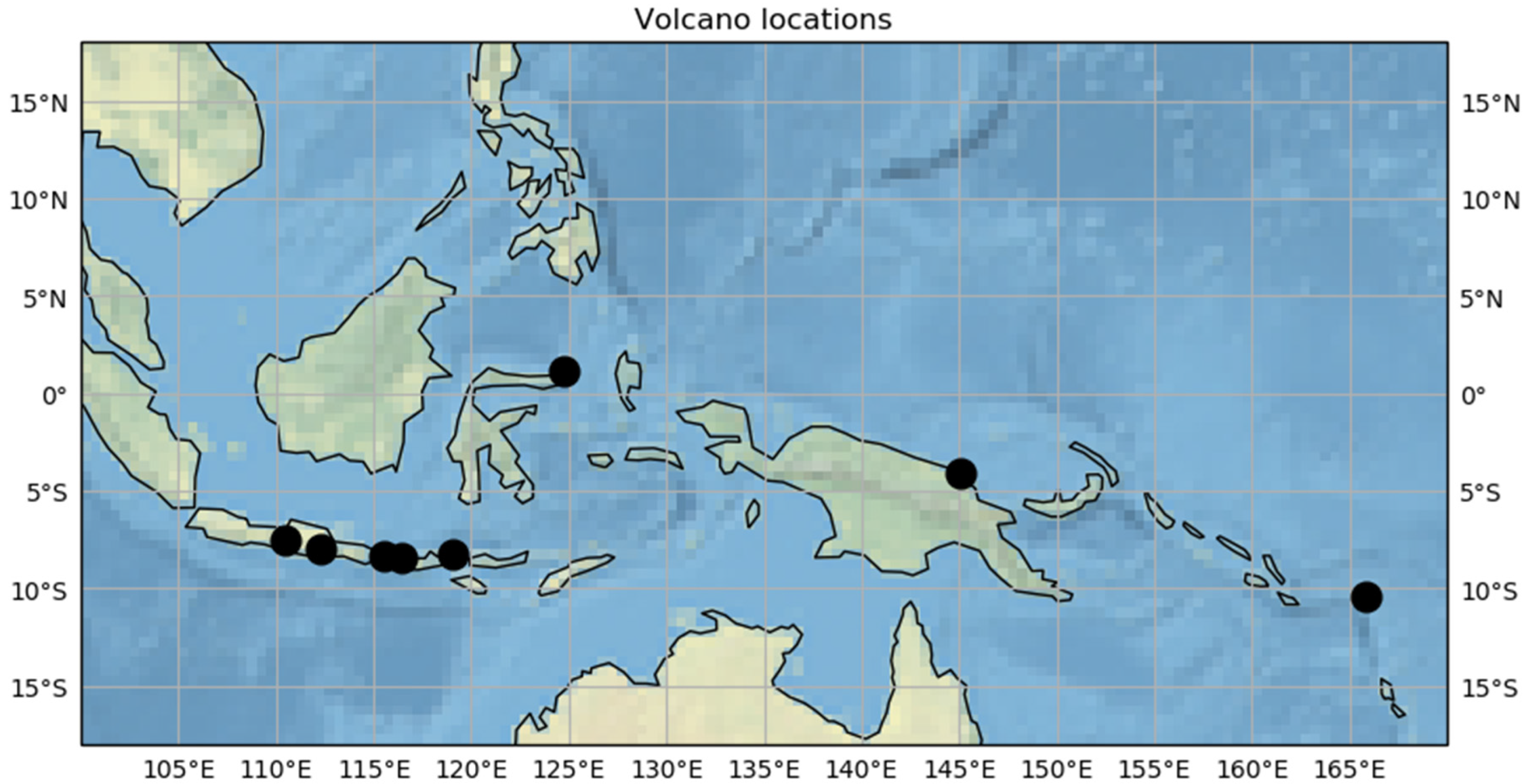
In this study, we investigated the utility of the different initialization schemes using a database of VOLCAT satellite retrieval data (Supplementary Materials) from 14 eruption case studies [27]. The eruption case studies are shown on a map in Figure 1 and also briefly described in Table 2.
In all model initialization methods described thus far, the model was perturbed by employing an ensemble of NWP fields to drive the dispersion model. In addition, the source term was also perturbed; this was done differently depending on the type of initialization model and observations being employed, as summarized in Table 1. In the cylindrical source model (SRC), the primary variable was randomly sampled over its uncertainty range, thus creating 10 samples for each NWP member. In the distal ash models (DIST, DIST(VARH)), the primary variables were the distal cloud initialization time , the maximum cloud top height , and the cloud depth , which were also randomly sampled. The number of samples depends on the number of available observations times; in general, it is ten times the number of available observations for each NWP field. We also considered a hybrid scheme (SRC-DIST) in which both cylindrical and distal initialization methods were employed. In this case the number of samples for each NWP member was twenty times the number of available observations. As a rough guide, with 24 NWP members and four observation times, this amounts to about 2000 ensemble members. These ensemble members were filtered relative to either the VOLCAT detections or the retrieved mass load, effective radius, and cloud top height fields in the analysis phase of the algorithm. In the forecast phase, the accepted members were propagated forward in time for the duration of the forecast. It should be noted that irrespective of whether detections or retrievals were used to filter the ensemble during the analysis phase, the results were always compared against the detailed retrieved data (and not just the detections) for verification purposes.
For the purposes of verification, we also performed reference runs relative to which the runs described above were evaluated. The reference runs replicated how the source is currently set up in many operational centers, such as VAAC Darwin. As described by Zidikheri and Lucas [3], it is a simple line source with uniform mass distribution in the vertical with the mass emission rate computed from the Mastin relationship [2] using a fine-ash fraction value of 0.05. The particle size distribution is a commonly used one in volcanic ash forecasting, originally based on the study of Hobbs [37,38]. The eruption height in the reference runs was a simple estimate obtained from satellite brightness temperatures, NWP model, and sounding temperature profiles, as is the common practice operationally. There was no representation of source-term uncertainty in the reference runs, but there was representation of NWP field uncertainty using the 24 ACCESS-GE ensemble members. Furthermore, ensemble filtering with respect to observations was not performed.
4. Results
4.1. General Verification Results
In what follows, we quantitatively compare the results obtained with the different model variant experiments listed in Table 1 (using either detections or retrievals) against the results obtained with reference runs. Both the experimental and reference runs were verified against VOLCAT retrieval data (mass load, effective radius, and cloud top height) for the 14 eruption case studies, listed in Section 3, using the Brier score (Equation (2)), which is a commonly used metric for verifying probabilistic forecasts. We then constructed a Brier skill score from the experimental Brier score (s) and reference Brier scores (). Given Brier scores range from 0 (best) to 1 (worst), positive skill score values imply model improvement relative to reference runs, while negative values imply model degradation relative to reference runs; small values close to 0 imply similar performance to reference runs [23].
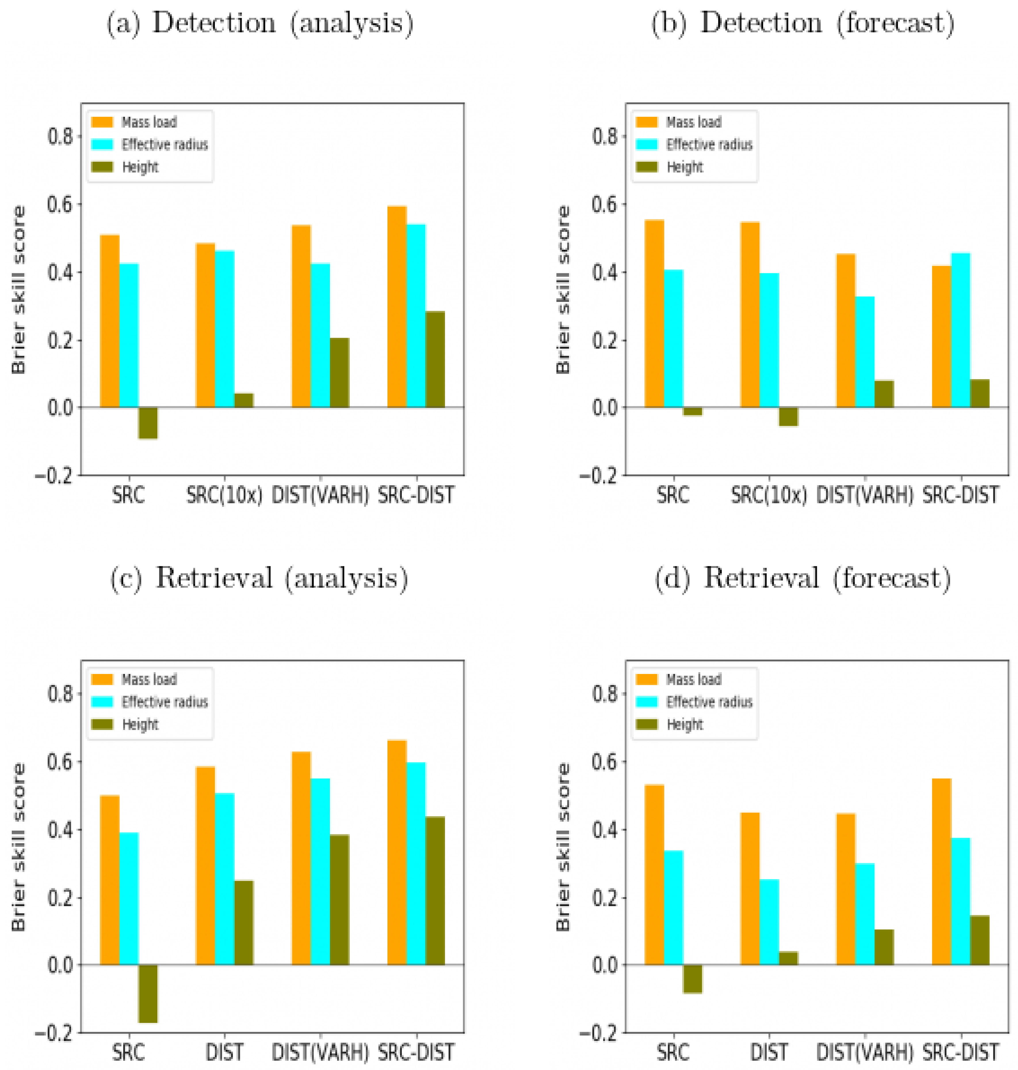
Figure 2 shows the median of the mass load, effective radius, and cloud-top height Brier skill scores obtained for all 14 eruption cases studies for different model variants. We can see that all ensemble filtered runs, irrespective of model variant, perform better than reference runs as far as mass load and effective radius are concerned. However, the cloud top height is slightly inferior to the reference when only the cylindrical source is used (although there is a slight improvement in the analysis phase when the number of ensemble members is increased in the detection optimized run (SRC(10×))). It is not completely clear why the cloud top height does not perform as well as the other fields; this issue is further discussed in Section 5. Whatever the cause, it is, however, clear from these results that with the use of the distal ash source there is improvement in the representation of the height field in the model. Further improvements can be achieved by adjusting the maximum cloud top height (i.e., the runs named as DIST(VARH)). Furthermore, it seems that the best improvement comes from using the hybrid scheme (SRC-DIST), in which both cylindrical and distal sources are employed in the initial ensemble prior to filtering. It is also clear from these results that the mass load field benefits the most from ensemble filtering. The only exception to this rule is for the hybrid source results (SRC-DIST) when no retrievals are available. In that case, the effective radius displays the most improvement.
Even though the benefits of employing the distal source are clear during the analysis phase, during the forecast phase it is not as clear that there is benefit in employing the distal source. Figure 2 shows that when only detections are used, it is only the cloud top height that is improved relative to the cylindrical source runs; the mass load field performs better with the cylindrical source and the effective radius results are mixed (poorer results with just the distal source and slight improvement with the hybrid scheme). In some sense, this is not surprising given that the mass and particle size distribution within the distal cloud can only be crudely represented in the absence of retrievals. When retrievals are used, there is improvement in all forecasted fields upon using the distal source within the hybrid scheme. On the face of it, these results imply that the distal source is only of benefit to quantitative estimates of ash cloud properties when retrievals are available, and when retrievals are not available only the cylindrical source should be employed. However, it should be remembered that the distal source formulation does improve the representation of ash location, as further discussed in Section 4.2, and this could be of benefit operationally even if the mass load estimates are not optimal. As noted in Table 1, the number of ensemble members used in the distal schemes (including the hybrid schemes) in general exceed the number of ensemble members used in the purely cylindrical source schemes by factors ranging from two to 11. To better understand the possible impact of ensemble size on the results, we employed the cylindrical source run with ten times the number of ensemble members in the standard run (i.e., an inflation factor of 10 in ensemble size), as noted in Table 1. We can see in Figure 2 that, although some of the skill scores differ slightly with larger ensemble size, there is no systematic trend in the skill scores with the larger ensemble size. The same conclusions may, therefore, be drawn about the relative performance of the distal source runs relative to the cylindrical source runs as for the runs with smaller ensemble size.
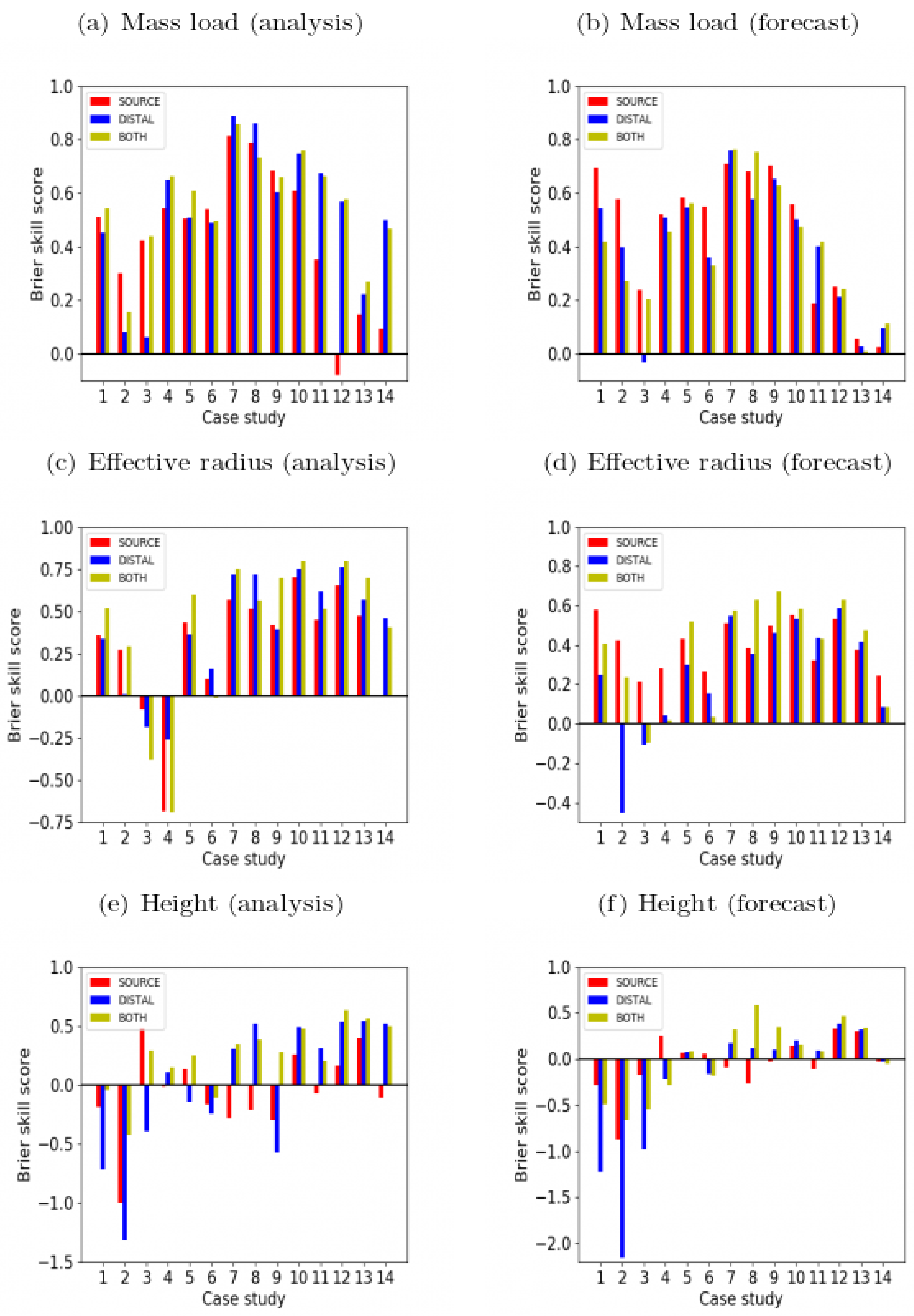
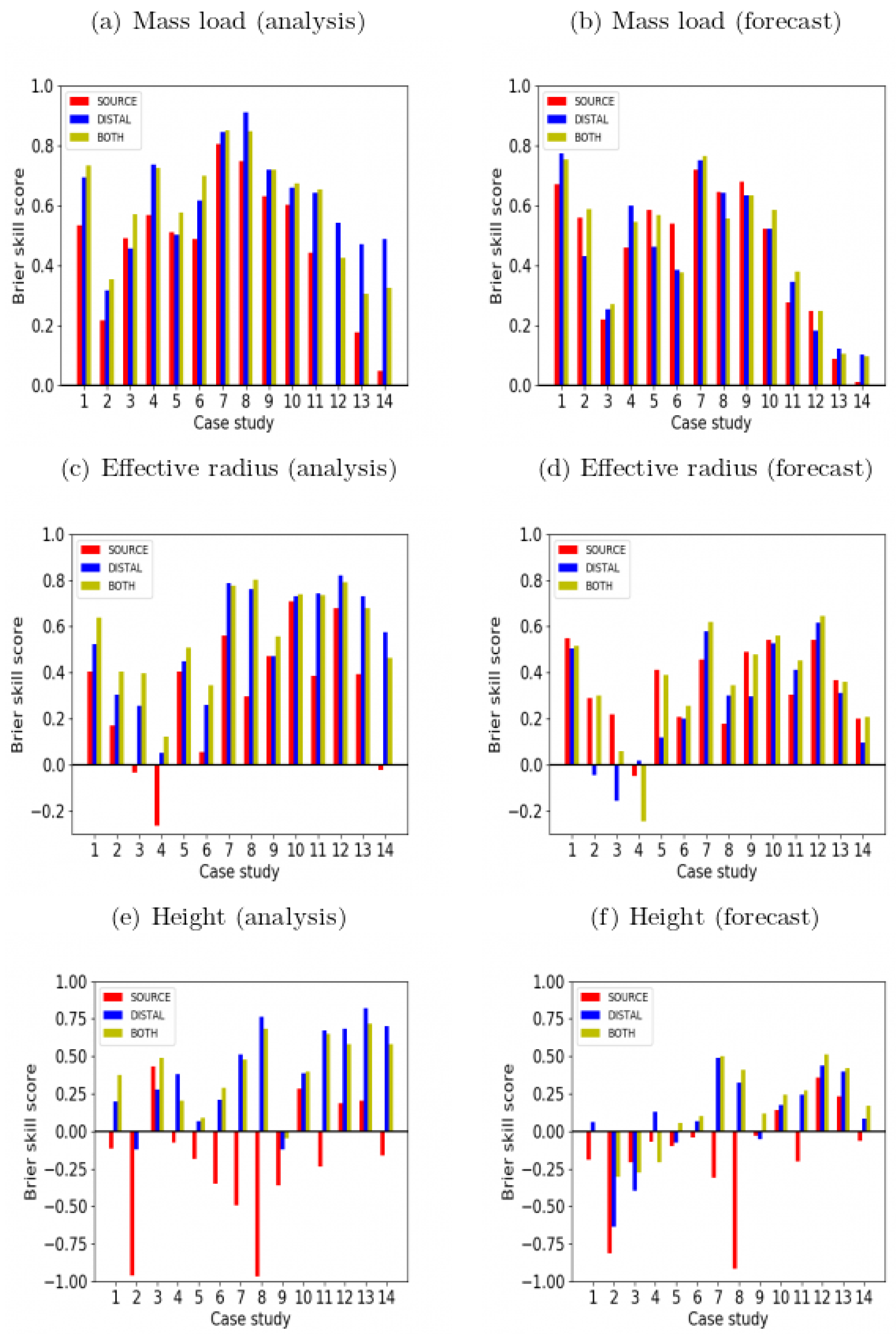
To better evaluate the utility of the distal source formulation, we examine the Brier skill scores for the individual case studies. Figure 3 shows the skill scores for all case studies when only detections are employed, while Figure 4 shows the skill scores when retrievals are employed. As alluded to by the median score results, generally the mass load field shows improvement in all cases. In the detection-based simulations, there are some exceptions, notably the Agung case when employing the SRC formulation during the analysis phase and the Manam I case when employing the DIST(VARH) formulation during the forecast phase. All case studies show improvement to the mass load field when retrievals are employed. Generally, employing the distal source, whether as purely distal (DIST(VARH)) or in a hybrid scheme (SRC-DIST), leads to significantly better results for the mass load field than for the cylindrical source during the analysis phase. During the forecast phase, the results are more mixed when employing detections, while lower-level eruptions utilizing distal sources perform better when initialized with retrievals.
Improvements to the effective radius field are not as consistent as for the mass field. We can see that, when employing the detection-based formulation, the effective radius in the Manam I, Tinakula, and Sangeang Api cases studies is outperformed by the reference runs. The effective radius in these case studies is somewhat improved when employing the retrievals, but it is still not consistently good. Apart from these case studies, there is improvement in the effective radius fields, particularly when retrievals are employed, which is reflected in the median skill scores shown in Figure 2. As discussed in the context of Figure 2, the cloud top height results are outperformed by the reference runs in some cases. This is particularly the case for the high-level eruptions (Kelut, Sangeang Api I, Manam I, and Tinakula). The results for some case studies are improved, particularly for the lower-level eruptions (Agung and Rinjani). The worst agreement generally occurs when employing the cylindrical source. Generally, there is some improvement to the cloud top height when employing the distal source, particularly during the analysis phase.
4.2. Comparison of Spatial Patterns for Selected Case Studies
In this section we compare the spatial patterns of mass load (effective radius and cloud top height patterns are discussed in Supplementary Materials) for two selected cases studies, namely the 13 February 2014 Kelut eruption, representing short-lived high-level eruptions, and the 4 November 2015 Rinjani eruption, representing low-level continuous eruptions. We compare patterns obtained from VOLCAT retrievals, reference runs, runs employing the cylindrical source formulation (SRC), runs employing the distal source formulation (SRC(VARH)), and runs employing the hybrid scheme (SRC-DIST).
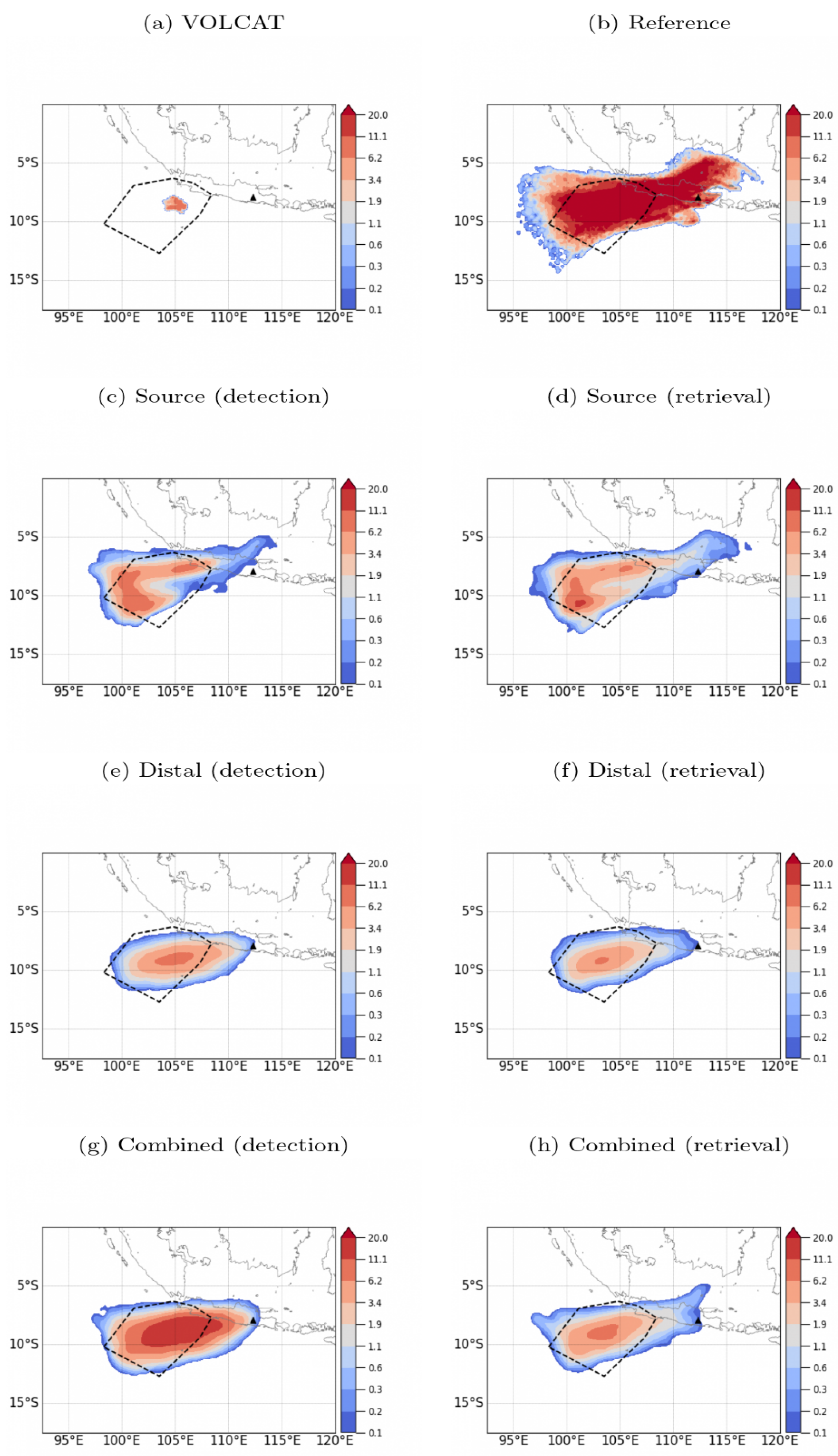
Figure 5 shows the mass load results for the Kelut case study at 14/0130 UTC; this timestep forms part of the analysis phase, which spans the period 13/2330–14/0230 UTC. The VOLCAT mass load retrieval at this timestep indicates a region of very high mass load close to the leading edge of the cloud to the west of the volcano. The mass loads in the near-source region are relatively small in comparison. The reference run (Figure 5b), on the other hand, indicates very high mass loads throughout the ash cloud, especially in the near-source region (exceeding 1000 g/m2 in some places). This pattern of disagreement, and its possible cause, has been discussed elsewhere in more detail [22]. The cylindrical source runs (SRC) (Figure 5c,d) model the distribution of mass quite well in agreement with the VOLCAT retrievals in both the detection and retrieval optimized version of the model.
There is a region in the retrievals (indicated by the dashed lines) that is not captured by the simulation in either the reference or SRC runs. Using the distal formulation (DIST(VARH)) leads to this missing region being quite well captured in both the detection and retrieval versions (Figure 5e,f). The hybrid model versions (SRC-DIST) also capture the missing region quite well. Surprisingly, the DIST(VARH) formulation (using only detections) can also capture the asymmetric distribution of mass to the west of the volcano (with more mass in the downstream region) even though there is no explicit assimilation of retrieved mass load data in this case. The corresponding run directly employing the retrievals also captures this asymmetric mass distribution well, but this is less surprising given the explicit insertion of retrieval data.
Figure 6 shows the results obtained at 14/0830 UTC, which occurs during the forecast phase (spanning 14/0330–14/0930 UTC). In this stage, there is no optimization with respect to observational data; the ensemble members retained by the filter during the analysis phase are simply propagated forward in time from the analysis. The VOLCAT retrieval at this timestep (and all timesteps after 14/0230 UTC) only indicates ash in a small region. This is almost certainly not the only region that contained significant amounts of ash. It is almost certain that the leading edge of the cloud at this time also contained significant amounts of ash, and this is supported by VAAC Darwin advisories during that period, as shown in Figure 6. The reference run predicts very high mass loads through the ash cloud (exceeding 20 g/m2); these are likely to be overestimates especially in the near-source region, as mass loads at those levels would almost certainly be picked up in satellite imagery, but the Darwin VAAC advisories only indicated ash further to the west of the volcano during the event [24]. The cylindrical source runs (SRC) predict high mass loads near the leading edge of the south-westward moving cloud and in the vicinity of the small region identified as containing ash by the retrievals, although this region appears to be somewhat to the north of the corresponding region in the retrievals. The distal source runs (DIST(VARH)) predict the location of ash identified by VOLCAT quite well in terms of magnitude and location. Surprisingly, the detection-based run predicts this region somewhat better than the retrieval-based run. The hybrid scheme (SRC-DIST) in this case produces patterns of mass distribution broadly like the purely distal (DIST(VARH)) runs. Again, the detection-base run appears to be broadly more consistent with the VOLCAT retrievals. The high mass load regions in the retrieval-based runs (and also the detection-based cylindrical source run) correspond quite well with the VAAC-drawn polygon.
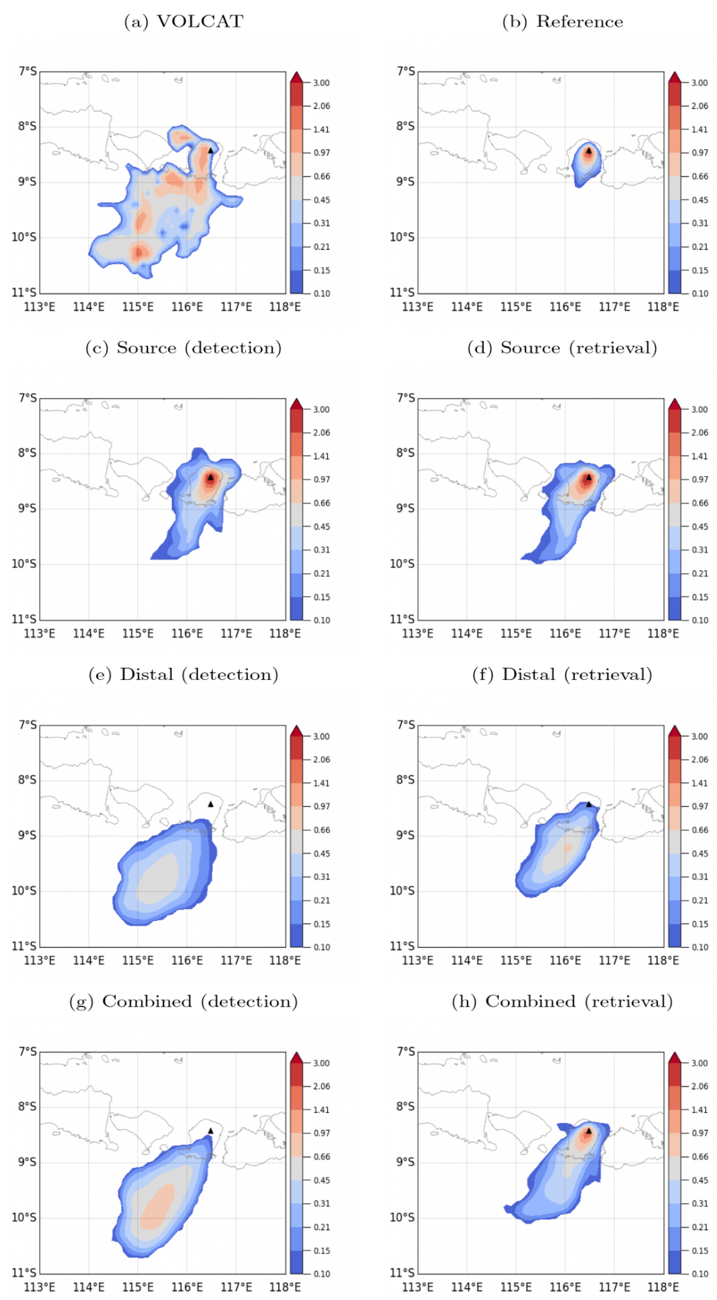
Figure 7 shows the results obtained for the 4 November 2015 Rinjani I case study at 5/0730 UTC (on 5 November, 19.5 h after the nominal start time of the eruption). This timestep forms part of the analysis phase of the simulations, which was set to be within the interval 5/0630 UTC–5/0930 UTC. The VOLCAT retrieval at this time shows more mass near the source compared to the downstream region, and the ash is transported in a south-west direction before turning more to the west. In the reference run, on the other hand, the ash is transported in a strict southward direction. Moreover, the ratio of mass in the near-source region to the mass retained in the downstream region is far greater than that in the VOLCAT retrieval. As a result, the cloud does not appear to extend south of 9° S; in fact, ash is present in the reference simulation south of 9° S, but it is at very low mass load levels (less than 0.1 g/m2). This is possibly related to the presence of a bigger proportion of large particles in the reference run, which would tend to lose mass due to surface deposition faster (see Section S2 of supplementary section). The ash transport in the cylindrical source runs (SRC) is significantly improved compared to the reference runs. Ash is transported in a south-west direction consistent with the satellite observations. However, there is still too little mass in the downstream region when compared to the observations. The transport of ash is further improved in the distal source formulation (DIST(VARH)). In the detection-based version, however, there is not enough mass in the near-source region and the spread of ash is somewhat greater than in the observations. The retrieval-based run does, on the other hand, agree quite well with the VOLCAT retrieval. The hybrid scheme (SRC-DIST) performs similarly to the purely distal source scheme in this case with some minor differences (ash cloud not as much spread out in the detection-based run and somewhat less mass downstream in the retrieval-based run).
Figure 8 shows the results from the Rinjani I case study at 5/1430 UTC. This occurs during the forecast phase, and it is five hours after the last analysis step; in this phase there is no optimization with respect to observations. The VOLCAT retrieval shows that ash has spread out more and has been transported further to the south-west. The mass is still dominated by ash in the near-source region, most likely due to the ongoing eruption, but there is considerable mass in the downstream region as well. The reference run does not perform very well; ash is still transported southward, instead of to the south-west, and there is very little mass south of 9° S. The cylindrical source runs (SRC) transport ash to the south-west consistent with observations, but there is still too little mass in the downstream region, especially south of 10° S. The ash coverage is significantly improved in the detection-based run in the distal source formulation (DIST(VARH)), but the near-source region contains too little mass. The retrieval-based run of the distal source formulation has a better representation of the near-source mass but is not as good at capturing the downstream region, which contains too little mass compared to the retrieval. The hybrid scheme (SRC-DIST) runs contain more mass in the near-source region, while also maintaining more mass in the downstream region.
5. Discussion
The focus of this study was to evaluate the utility of employing a direct satellite data insertion approach to improve the performance of a volcanic ash ensemble forecasting system. This system, which is described by Zidikheri and Lucas [24], employs an ensemble filtering scheme to optimize forecasts. It has two distinct phases, namely the analysis and forecast phases. During the analysis phase, ensemble members that represent the uncertainty in the source term and meteorological fields are created and either accepted or rejected by the filter based on their degree of agreement with remotely sensed satellite observations available at the time of the forecast. The accepted members are then used in the forecast phase to predict the future evolution of the ash cloud.
In the original system described by Zidikheri and Lucas [24], the source term comprises a cylinder of particles with diameters ranging from 0–100 m bounded at the base by the volcano summit and at the top by the eruption height. The distribution of mass in the vertical is assumed to be Gaussian and the distribution among different particle sizes to be log normal. The source term uncertainties are determined by the uncertainty in the eruption height. Although other source parameters (describing vertical and particle size mass distributions) are also important, they are determined from empirical parameterizations that are dependent on the eruption height [3]. That makes the eruption height the sole independent parameter that determines source term variability. The method was shown to work quite well even when satellite retrievals were not available in real-time to filter the ensemble members. In that case, it was shown that manually determined ash location polygons could be used instead. Even though the cylindrical source representation works quite well in many cases, it is a very simple representation of very complex near-source processes and is, therefore, limited in that regard. In addition, it is problematic to apply in long-lived eruptions where the time difference between the start of the eruption and the period of interest to be forecasted is very long. In those situations, we expect significant errors due to both the extreme simplicity of the cylindrical source formulation and meteorological field errors.
In this study, we expanded our observational field to include not only the mass loads, as was done in previous studies, but to also include the effective radius and cloud top height fields. The results confirmed that, when employing the cylindrical source formulation, both the mass load and effective radius forecast fields agree better with the retrievals than the corresponding fields obtained from reference runs. The reference runs employ a vertically uniform line source with mass emission rate determined from the Mastin relationship [2] and a default particle size distribution based on the study of Hobbs [37]. However, it was found that the cloud top heights obtained were in fact, on average, inferior to the cloud top heights in the reference runs. We also developed another representation of the source term that is based on directly inserting the satellite observations. The advantage of this approach is that recent satellite observations can be directly ingested into the model and propagated forward in time over the period of interest instead of relying on the model to carry the particles from the source. In this distal source formulation, the horizontal boundaries of the ash cloud are determined by the satellite observations, which can be detailed retrievals or simple detections. When retrievals are available, the mass load and effective radius fields are used to compute the total mass and size distribution of ash within the cloud, assuming uniformity over the depth of the cloud. When only detections are available, then empirical parametrizations used for the cylindrical source are used to infer the total mass and size distribution within the cloud.
In the distal ash formulation, the cloud top is assumed to be uniform over the whole cloud when detections are used and treated as a variable parameter to be optimized by ensemble filtering; this is like how the eruption height is treated in the cylindrical source formulation. When retrievals are used, the cloud top is a scaled version of the satellite retrieved cloud top; the maximum cloud top height is treated as the variable parameter in this case. The cloud thickness in both cases is also treated as a poorly known parameter that is optimized by the application of the ensemble filter. Finally, the initialization time is also treated as an uncertain parameter to be optimized by ensemble filtering. This effectively means that the appropriate satellite observation used to initialize the model is not chosen a priori, but it is randomly chosen from a sample of available observations. The ensemble then contains a range of possible observations that are used as distal sources. The motivation for this approach is to ameliorate the effect of observational random errors on the forecast. This approach requires a minimum of two observations to work—one for initialization and one for optimization—but will clearly work better with more observations. Because of all these uncertainties, the distal source formulation is more computationally demanding even though the simulation run time for each ensemble member is shortened. This is because it requires sampling over at least three dimensions (top height, thickness, and start time) compared to the cylindrical source formulation that requires only sampling of the eruption height.
We found that, on average, the distal source formulation unambiguously improved the results during the analysis phase of the algorithm. Most fields performed better relative to observations (in both detection and retrieval-based initialization approaches) compared to the corresponding fields in the reference runs. This was also true for the cloud top height, which was shown to be superior on average to the reference run in contrast to the results obtained with the cylindrical source. During the forecast phase, however, only the cloud top heights were better on average than the cloud top heights obtained from the cylindrical source runs, although all fields outperformed the reference run fields. On the face of it, these results suggest that the distal source formulation is ultimately of limited utility (given that it is also computationally more intensive) except possibly for the representation of the cloud top height. However, a closer inspection of individual case studies revealed that the distal source can provide additional forecast skill, particularly for longer-lived, low-level, eruptions such as the November 2015 Rinjani eruptions. In those situations, it is difficult to model the transport of ash from the eruption start time to the period of interest for the forecasts using the simple cylindrical source. It appears that the transport of ash is better represented in the forecasts when the models are initialized by a distal ash closer in time to the forecasted period in those cases.
Although the distal source formulation can ameliorate errors arising from NWP and source errors, particularly when the start of the forecasting period occurs much later than the eruption start time, in some situations the use of satellite information alone might be deleterious to the forecast performance. This could occur if the satellite retrieved field has systematic errors or if the satellite imagery does not represent the complete ash cloud coverage due to detection errors and meteorological cloud cover. For this reason, we have also considered in this study a hybrid scheme in which some ensemble members are generated by cylindrical sources, while others are generated by distal sources. This attempts to find a middle ground to minimize the chance of the system performing poorly in operational contexts because the optimal source formulation was not used for a particular situation.
The verification results indicate that the hybrid scheme outperforms the reference, cylindrical source, and distal source runs for all field types during the analysis phase irrespective of whether detections or retrievals are used. During the forecast phase, the hybrid scheme outperforms the reference runs, but it is outperformed by the cylindrical source and purely distal source schemes as far as mass load is concerned when employing only detections. The hybrid scheme still outperforms the other schemes as far as effective radius and cloud top height is concerned. When retrievals are used, the hybrid scheme outperforms all other schemes for all field types. These results suggest that the hybrid scheme is likely to be of most utility when retrievals are available. When only detections are available, it may still provide useful improvements to the forecasts of ash transport in long-lived, low-level eruptions, although the mass loads may not necessarily be very accurate. It should be remembered, however, that both the hybrid and distal source schemes are more computationally expensive to run, and they, therefore, are more likely to be of use for the purposes of refining an initial forecast rather than to be used routinely.
The experiments reported in this paper were run on the Australian National Computing Infrastructure (NCI) cluster. However, the code running on NCI was not optimized to run efficiently. Since these experiments were performed, we have significantly improved the code and optimized it to run pre-operationally on the Bureau of Meteorology’s Cray XC40 development supercomputer (named Terra). In its current stage of development, the system runs 100 ensemble members in parallel on Terra, which leads to substantial improvement in run times. For example, using the Kelut case study (one of the case studies in this paper), the SRC run (using 216 ensemble members in the pre-operational version) typically runs in under 15 min on Terra. The more computationally intensive SRC-DIST run (using 1296 analysis ensemble members in the pre-operational version) typically runs in just under 30 min. With more hardware upgrades planned in the coming years, we expect further improvement in run times.
6. Conclusions
Direct insertion of satellite data was found to have a positive impact on skill scores of an ensemble volcanic ash forecasting model when applied to a dataset of 14 eruption case studies in the tropics. The most consistent improvement of skill scores was demonstrated in a hybrid scheme in which some ensemble members were initialized by a cylindrical source, while other ensemble members were initialized by a distal source based on direct insertion of data. Furthermore, the best skill scores were obtained when satellite retrievals of ash mass load, effective radius, and cloud top height were used. However, skill scores obtained from simulations employing only satellite ash detections were still superior to skill scores obtained from reference runs employing model configurations like those used in current operational volcanic ash forecasting models.
Supplementary Materials
VOLCAT satellite retrieval data used in this study are available at http://doi.org/10.5281/zenodo.3579613.
Author Contributions
Conceptualization, M.J.Z.; methodology, M.J.Z.; software, M.J.Z.; validation, M.J.Z.; formal analysis, M.J.Z.; investigation, M.J.Z.; resources, M.J.Z. and C.L.; data curation, M.J.Z. and C.L.; writing—original draft preparation, M.J.Z.; writing—review and editing, M.J.Z.; visualization, M.J.Z.; project administration, C.L. All authors have read and agreed to the published version of the manuscript.
Funding
This research received no external funding.
Institutional Review Board Statement
Not applicable.
Informed Consent Statement
Not applicable.
Data Availability Statement
ACCESS-GE model data used in this study (in HYSPLIT ARL format) can be downloaded from https://dx.doi.org/10.25914/6142ad42d977e (accessed on 12 September 2021) and VOLCAT satellite retrieval data can be downloaded from http://doi.org/10.5281/zenodo.3579613 (accessed on 12 September 2021).
Acknowledgments
We would like to thank Richard Dare and Rodney Potts, both from the Bureau of Meteorology, for reviewing the first draft of this paper and providing useful comments. Richard Dare also provided fall speed data based on the Ganser formula that we used to evaluate possible errors in the Stokes formula, which was used to estimate the mass remaining in a distal cloud as discussed in Section 2.3.2 of this paper. We also acknowledge valuable comments from three reviewers, which were integrated into the revised version of this paper.
Conflicts of Interest
The authors declare no conflict of interest.
References
- Casadevall, T.J. Volcanic Ash and Aviation Safety: Proceedings of the First International Symposium on Volcanic Ash and Aviation Safety; US Government Printing Office: Washington, DC, USA, 1994.
- Mastin, L.; Guffanti, M.; Servranckx, R.; Webley, P.; Barsotti, S.; Dean, K.; Durant, A.; Ewert, J.; Neri, A.; Rose, W.; et al. A multidisciplinary effort to assign realistic source parameters to models of volcanic ash-cloud transport and dispersion during eruptions. J. Volcanol. Geotherm. Res. 2009, 186, 10–21. [Google Scholar] [CrossRef]
- Zidikheri, M.J.; Lucas, C. Using Satellite Data to Determine Empirical Relationships between Volcanic Ash Source Parameters. Atmosphere 2020, 11, 342. [Google Scholar] [CrossRef] [Green Version]
- Bessho, K.; Date, K.; Hayashi, M.; Ikeda, A.; Imai, T.; Inoue, H.; Kumagai, Y.; Miyakawa, T.; Murata, H.; Ohno, T.; et al. An introduction to Himawari-8/9—Japan’s new-generation geostationary meteorological satellites. J. Meteorol. Soc. Japan. Ser. II 2016, 94, 151–183. [Google Scholar] [CrossRef] [Green Version]
- Corradini, S.; Merucci, L.; Prata, F.; Piscini, A. Volcanic ash and SO2in the 2008 Kasatochi eruption: Retrievals comparison from different IR satellite sensors. J. Geophys. Res. Space Phys. 2010, 115, D2. [Google Scholar] [CrossRef]
- Francis, P.N.; Cooke, M.C.; Saunders, R.W. Retrieval of physical properties of volcanic ash using Meteosat: A case study from the 2010 Eyjafjallajökull eruption. J. Geophys. Res. Space Phys. 2012, 117, D20. [Google Scholar] [CrossRef]
- Pavolonis, M.J.; Heidinger, A.; Sieglaff, J.M. Automated retrievals of volcanic ash and dust cloud properties from upwelling infrared measurements. J. Geophys. Res. Atmos. 2013, 118, 1436–1458. [Google Scholar] [CrossRef]
- Pavolonis, M.J.; Sieglaff, J.M.; Cintineo, J. Spectrally Enhanced Cloud Objects—A generalized framework for automated detection of volcanic ash and dust clouds using passive satellite measurements: 1. Multispectral analysis. J. Geophys. Res. Atmos. 2015, 120, 7813–7841. [Google Scholar] [CrossRef]
- Pavolonis, M.J.; Sieglaff, J.M.; Cintineo, J. Spectrally Enhanced Cloud Objects—A generalized framework for automated detection of volcanic ash and dust clouds using passive satellite measurements: 2. Cloud object analysis and global application. J. Geophys. Res. Atmos. 2015, 120, 7842–7870. [Google Scholar] [CrossRef]
- Eckhardt, S.; Prata, A.J.; Seibert, P.; Stebel, K.; Stohl, A. Estimation of the vertical profile of sulfur dioxide injection into the atmosphere by a volcanic eruption using satellite column measurements and inverse transport modeling. Atmos. Chem. Phys. Discuss. 2008, 8, 3881–3897. [Google Scholar] [CrossRef] [Green Version]
- Kristiansen, N.I.; Stohl, A.; Prata, F.; Richter, A.; Eckhardt, S.; Seibert, P.; Hoffmann, A.; Ritter, C.; Bitar, L.; Duck, T.J.; et al. Remote sensing and inverse transport modeling of the Kasatochi eruption sulfur dioxide cloud. J. Geophys. Res. Space Phys. 2010, 115, D2. [Google Scholar] [CrossRef]
- Stohl, A.; Prata, A.J.; Eckhardt, S.; Clarisse, L.; Durant, A.; Henne, S.; Kristiansen, N.I.; Minikin, A.; Schumann, U.; Seibert, P.; et al. Determination of time- and height-resolved volcanic ash emissions and their use for quantitative ash dispersion modeling: The 2010 Eyjafjallajökull eruption. Atmos. Chem. Phys. Discuss. 2011, 11, 4333–4351. [Google Scholar] [CrossRef] [Green Version]
- Seibert, P.; Kristiansen, N.I.; Richter, A.; Eckhardt, S.; Prata, A.J.; Stohl, A. Uncertainties in the inverse modelling of sulphur dioxide eruption profiles. Geomat. Nat. Hazards Risk 2011, 2, 201–216. [Google Scholar] [CrossRef]
- Boichu, M.; Menut, L.; Khvorostyanov, D.; Clarisse, L.; Clerbaux, C.; Turquety, S.; Coheur, P.-F. Inverting for volcanic SO2 flux at high temporal resolution using spaceborne plume imagery and chemistry-transport modelling: The 2010 Eyjafjallajökull eruption case study. Atmos. Chem. Phys. Discuss. 2013, 13, 8569–8584. [Google Scholar] [CrossRef] [Green Version]
- Boichu, M.; Clarisse, L.; Khvorostyanov, D.; Clerbaux, C. Improving volcanic sulfur dioxide cloud dispersal forecasts by progressive assimilation of satellite observations. Geophys. Res. Lett. 2014, 41, 2637–2643. [Google Scholar] [CrossRef] [Green Version]
- Zidikheri, M.J.; Potts, R.; Lucas, C. A probabilistic inverse method for volcanic ash dispersion modelling. ANZIAM J. 2016, 55, 194–209. [Google Scholar] [CrossRef] [Green Version]
- Moxnes, E.D.; Kristiansen, N.I.; Stohl, A.; Clarisse, L.; Durant, A.; Weber, K.; Vogel, A. Separation of ash and sulfur dioxide during the 2011 Grímsvötn eruption. J. Geophys. Res. Atmos. 2014, 119, 7477–7501. [Google Scholar] [CrossRef] [Green Version]
- Kristiansen, N.I.; Prata, A.J.; Stohl, A.; Carn, S.A. Stratospheric volcanic ash emissions from the 13 February 2014 Kelut eruption. Geophys. Res. Lett. 2015, 42, 588–596. [Google Scholar] [CrossRef] [Green Version]
- Zidikheri, M.J.; Potts, R.J. A simple inversion method for determining optimal dispersion model parameters from satellite detections of volcanic sulfur dioxide. J. Geophys. Res. Atmos. 2015, 120, 9702–9717. [Google Scholar] [CrossRef]
- Chai, T.; Crawford, A.; Stunder, B.; Pavolonis, M.J.; Draxler, R.; Stein, A. Improving volcanic ash predictions with the HYSPLIT dispersion model by assimilating MODIS satellite retrievals. Atmos. Chem. Phys. Discuss. 2017, 17, 2865–2879. [Google Scholar] [CrossRef] [Green Version]
- Zidikheri, M.J.; Lucas, C.; Potts, R.J. Estimation of optimal dispersion model source parameters using satellite detections of volcanic ash. J. Geophys. Res. Atmos. 2017, 122, 8207–8232. [Google Scholar] [CrossRef]
- Zidikheri, M.J.; Lucas, C.; Potts, R.J. Toward quantitative forecasts of volcanic ash dispersal: Using satellite retrievals for optimal estimation of source terms. J. Geophys. Res. Atmos. 2017, 122, 8187–8206. [Google Scholar] [CrossRef]
- Zidikheri, M.J.; Lucas, C.; Potts, R.J. Quantitative Verification and Calibration of Volcanic Ash Ensemble Forecasts Using Satellite Data. J. Geophys. Res. Atmos. 2018, 123, 4135–4156. [Google Scholar] [CrossRef]
- Zidikheri, M.J.; Lucas, C. A Computationally Efficient Ensemble Filtering Scheme for Quantitative Volcanic Ash Forecasts. J. Geophys. Res. Atmos. 2021, 126, e2020JD033094. [Google Scholar] [CrossRef]
- Harvey, N.; Dacre, H.; Webster, H.; Taylor, I.; Khanal, S.; Grainger, R.; Cooke, M. The Impact of Ensemble Meteorology on Inverse Modeling Estimates of Volcano Emissions and Ash Dispersion Forecasts: Grímsvötn 2011. Atmosphere 2020, 11, 1022. [Google Scholar] [CrossRef]
- Lucas, C.; Majewski, L. Evaluation of GEOCAT Volcanic Ash Algorithm for Use in BoM—A Report of the Improved Volcanic Ash Detection and Prediction Project; Bureau Research Report 004; Bureau of Meteorology: Melbourne, Australia, 2015. [Google Scholar]
- Lucas, C.; Zidikheri, M.J. Volcat Satellite Retrievals for Selected Case Studies. 2019. Available online: http://doi.org/10.5281/zenodo.3579613 (accessed on 15 September 2021).
- Wilkins, K.L.; Mackie, S.; Watson, M.; Webster, H.N.; Thomson, D.J.; Dacre, H.F. Data insertion in volcanic ash cloud forecasting. Ann. Geophys. 2015, 57, 24. [Google Scholar] [CrossRef]
- Wilkins, K.L.; Watson, I.M.; Kristiansen, N.I.; Webster, H.N.; Thomson, D.J.; Dacre, H.F.; Prata, A.J. Using data insertion with the NAME model to simulate the 8 May 2010 Eyjafjallajökull volcanic ash cloud. J. Geophys. Res. Atmos. 2015, 121, 306–323. [Google Scholar] [CrossRef] [Green Version]
- Wilkins, K.; Western, L.; Watson, I. Simulating atmospheric transport of the 2011 Grímsvötn ash cloud using a data insertion update scheme. Atmos. Environ. 2016, 141, 48–59. [Google Scholar] [CrossRef] [Green Version]
- Draxler, R.R.; Hess, G.D. An overview of the HYSPLIT_4 modelling system for trajectories. Aust. Meteorol. Mag. 1998, 47, 295–308. [Google Scholar]
- O’Kane, T.J.; Naughton, M.J.; Xiao, Y. The Australian community climate and earth system simulator global and regional ensemble prediction scheme. ANZIAM J. 2008, 50, 385–398. [Google Scholar] [CrossRef] [Green Version]
- Dare, R.A.; Smith, D.H.; Naughton, M.J. Ensemble Prediction of the Dispersion of Volcanic Ash from the 13 February 2014 Eruption of Kelut, Indonesia. J. Appl. Meteorol. Clim. 2016, 55, 61–78. [Google Scholar] [CrossRef]
- Dare, R.A. Sedimentation of Volcanic Ash in the HYSPLIT Dispersion Model; Centre for Australian Weather and Climate Research: Melbourne, Australia, 2015. [Google Scholar]
- Ganser, G.H. A rational approach to drag prediction of spherical and nonspherical particles. Powder Technol. 1993, 77, 143–152. [Google Scholar] [CrossRef]
- Prata, A.J.; Prata, A.T. Eyjafjallajökull volcanic ash concentrations determined using Spin Enhanced Visible and Infrared Imager measurements. J. Geophys. Res. Space Phys. 2012, 117, 23. [Google Scholar] [CrossRef] [Green Version]
- Hobbs, P.V.; Radke, L.F.; Lyons, J.H.; Ferek, R.J.; Coffman, D.J.; Casadevall, T.J. Airborne measurements of particle and gas emissions from the 1990 volcanic eruptions of Mount Redoubt. J. Geophys. Res. Space Phys. 1991, 96, 18735–18752. [Google Scholar] [CrossRef] [Green Version]
- Webster, H.N.; Thomson, D.J.; Johnson, B.T.; Heard, I.P.C.; Turnbull, K.; Marenco, F.; Kristiansen, N.I.; Dorsey, J.; Minikin, A.; Weinzierl, B.; et al. Operational prediction of ash concentrations in the distal volcanic cloud from the 2010 Eyjafjallajökull eruption. J. Geophys. Res. Space Phys. 2012, 117, D20. [Google Scholar] [CrossRef] [Green Version]
Figure 1.
Map showing the locations of volcanoes used as case studies in this paper (black dots).

Figure 2.
Brier skill scores of ash mass load, effective radius, and cloud top height averaged over 14 eruption case studies for (a) detection-based analyses, (b) detection-based forecasts, (c) retrieval-based analyses, and (d) retrieval-based forecasts. Different initialization methods (SRC, SRC(10×), DIST, DIST(VARH), and SRC-DIST) are considered for each of these runs, as further described in Table 1.

Figure 3.
Brier skill scores obtained for 14 different eruption case studies using detection-based initialization and optimization: (a) Mass load analyses, (b) mass load forecasts, (c) effective radius analyses, (d) effective radius forecasts, (e) cloud top height analyses, and (f) cloud top height forecasts. Note that, even though only the detections are used for initialization and optimization, the full VOLCAT retrievals are used to compute the Brier skill scores here. The case studies numbered 1 to 14 are described in more detail in Section 3 and in Zidikheri and Lucas (2020). They are (1) Kelut, (2) Sangeang Api I, (3) Manam I, (4) Tinakula, (5) Sangeang Api II, (6) Manam II, (7) Soputan I, (8) Soputan II, (9) Sangeang Api III, (10) Merapi, (11) Rinjani III, (12) Agung, (13) Rinjani I, and (14) Rinjani II; the roman numerals indicate the time sequence for eruptions from the same volcano. Results for three different initialization methods are shown, namely cylindrical source, distal (with top height varied), and ‘both’, which uses a mixed approach in which some ensemble members are initialized by the cylindrical source, while others are initialized from the distal source.

Figure 4.
Brier skill scores obtained for 14 different eruption case studies using retrieval-based initialization and optimization. Other details are the same as in Figure 2.
Figure 4.
Brier skill scores obtained for 14 different eruption case studies using retrieval-based initialization and optimization. Other details are the same as in Figure 2.

Figure 5.
Mass load fields (in g/m2) in the 13 February 2014 Kelut eruption case study at 14/0130 UTC for (a) VOLCAT retrieval, (b) reference run, (c) cylindrical source run with detection-based optimization, (d) cylindrical source run with retrieval-based optimizations, (e) distal source run with detection-based initialization and optimization, (f) distal source run with retrieval-based initialization and optimization, (g) hybrid source run using detections, and (g) hybrid source run using retrievals. The fields in (b–h) are ensemble means. The dashed lines indicate a region of interest discussed in the text.

Figure 6.
Mass load fields (in g/m2) obtained for the 13 February 2014 Kelut eruption case study at 14/0830 UTC. The explanation for the different panels is the same as in Figure 5. The dashed lines represent the Darwin VAAC polygon at 14/0830 UTC.
Figure 6.
Mass load fields (in g/m2) obtained for the 13 February 2014 Kelut eruption case study at 14/0830 UTC. The explanation for the different panels is the same as in Figure 5. The dashed lines represent the Darwin VAAC polygon at 14/0830 UTC.

Figure 7.
Mass load fields (in g/m2) in the 4 November 2015 Rinjani eruption case study at 5/0730 UTC for (a) VOLCAT retrieval, (b) reference run, (c) cylindrical source run with detection-based optimization, (d) cylindrical source run with retrieval-based optimizations, (e) distal source run with detection-based initialization and optimization, (f) distal source run with retrieval-based initialization and optimization, (g) hybrid source run using detections, and (g) hybrid source run using retrievals. The mass loads in (b–h) are ensemble means.

Figure 8.
Mass load fields (in g/m2) in the 4 November 2015 Rinjani eruption case study at 5/1430 UTC. The other details are the same as in Figure 7.
Figure 8.
Mass load fields (in g/m2) in the 4 November 2015 Rinjani eruption case study at 5/1430 UTC. The other details are the same as in Figure 7.


Table 1.
A summary of the different model initialization methods (each associated with either satellite-based retrievals or detections), type of filtering observations, variable independent parameters, and the number of ensemble members used during the analysis phase in this study. The second number in brackets for the cylinder source in the last column indicates that more ensemble members were used in a few case studies. In these case studies, in which ash was released continuously over a period of several days, not only was the eruption height varied but so was the start time. This was done because the eruption start time was several days in the past relative to available observations and, therefore, it was not viable to start the simulation at the eruption start time. This approach is described in detail by Zidikheri et al. [23].
| Variant Name | Initialization Type | Filtering Observations | Sampled (Variable) Parameters | Number of Analysis Ensemble Members | |
|---|---|---|---|---|---|
| 1 | SRC (retrieval) | Cylinder source | Retrievals and detections | Cloud top height ( | 240 (720) |
| 2 | SRC (detection) | Cylinder source | Detections | Same as 1 | Same as 1 |
| 3 | DIST (retrieval) | Distal (retrieval; top height fixed) | Retrievals and detections | Initial time ( Cloud thickness () | 480–1200 |
| 4 | DIST(VARH) (retrieval) | Distal (retrieval; top height varied) | Retrievals and detections | Initial time ( Cloud top height ( Cloud thickness () | Same as 3 |
| 5 | DIST(VARH) (detection) | Distal (top height varied) | Detections | Same as 4 | Same as 3 |
| 6 | SRC-DIST (retrieval) | Cylinder source and distal (retrieval; top height varied) | Retrievals and detections | Same as 4 | 1200–2640 |
| 7 | SRC-DIST (detection) | Cylinder source and distal (detection; top height varied) | Detections | Same as 4 | 1200–2640 |
| 8 | SRC(10×) | Cylinder source | Detections | Same as 1, 2 | 2400 (7200) |
| 9 | Reference | Simple line source | - | - | 24 |
Table 2.
A brief description of the eruption case studies used in this paper. The eruption duration values are the ones used in the model. These are rough estimates based on inspection of satellite imagery. For cases studies prior to 2016, the frequency of satellite data was 1 h, so duration estimates shorter than this were not possible. For the Rinjani I and II case studies, the eruption was ongoing and, therefore, the eruption duration was set equal to the simulation duration.
| Index | Volcano | Location | Eruption Time and Date | Approx. Duration (h) | Estimated Height (km a.s.l.) |
|---|---|---|---|---|---|
| 1 | Kelut | 112.31° E, 7.93° S | 1600Z/13/02/2014 | 3.0 | 26 |
| 2 | Sangeang Api I | 119.07° E, 8.20° S | 0800Z/30/05/2014 | 1.0 | 15–20 |
| 3 | Manam | 145.04° E, 4.08° S | 0130Z/31/07/2015 | 1.0 | 20 |
| 4 | Tinakula | 165.80° E, 10.38° S | 2330Z/20/10/2017 | 1.0 | 17 |
| 5 | Sangeang Api II | Same as 2 | 1700Z/30/05/2014 | 1.0 | 15–16 |
| 6 | Manam | Same as 3 | 0300Z/08/12/2018 | 3.0 | 13–14 |
| 7 | Soputan I | 124.73° E, 1.11° N | 2240Z/04/01/2016 | 1.0 | 12–13 |
| 8 | Soputan II | Same as 7 | 0600Z/05/01/2016 | 1.0 | 12–13 |
| 9 | Sangeang Api III | Same as 2, 5 | 2000Z/30/05/2014 | 1.0 | 14–15 |
| 10 | Merapi | 110.44° E, 7.54° S | 0030Z/11/05/2018 | 2.5 | 8 |
| 11 | Rinjani III | 116.47° E, 8.42° S | 0300Z/01/08/2016 | 1.0 | 6–10 |
| 12 | Agung | 115.51° E, 8.34° S | 1130Z/24/05/2019 | 0.5 | 6–7 |
| 13 | Rinjani I | Same as 11 | 1200Z/04/11/2015 | 48.0 | 6 |
| 14 | Rinjani II | Same as 11, 13 | 0000Z/05/11/2015 | 48.0 | 6 |
Publisher’s Note: MDPI stays neutral with regard to jurisdictional claims in published maps and institutional affiliations. |
© 2021 by the authors. Licensee MDPI, Basel, Switzerland. This article is an open access article distributed under the terms and conditions of the Creative Commons Attribution (CC BY) license (https://creativecommons.org/licenses/by/4.0/).
Share and Cite
MDPI and ACS Style
Zidikheri, M.J.; Lucas, C. Improving Ensemble Volcanic Ash Forecasts by Direct Insertion of Satellite Data and Ensemble Filtering. Atmosphere 2021, 12, 1215. https://doi.org/10.3390/atmos12091215
AMA Style
Zidikheri MJ, Lucas C. Improving Ensemble Volcanic Ash Forecasts by Direct Insertion of Satellite Data and Ensemble Filtering. Atmosphere. 2021; 12(9):1215. https://doi.org/10.3390/atmos12091215
Chicago/Turabian StyleZidikheri, Meelis J., and Chris Lucas. 2021. "Improving Ensemble Volcanic Ash Forecasts by Direct Insertion of Satellite Data and Ensemble Filtering" Atmosphere 12, no. 9: 1215. https://doi.org/10.3390/atmos12091215
Note that from the first issue of 2016, this journal uses article numbers instead of page numbers. See further details here.