
Recognizing human activities in Industry 4.0 scenarios through an analysis-modeling- recognition algorithm and context labels
Abstract
Activity recognition technologies only present a good performance in controlled conditions, where a limited number of actions are allowed. On the contrary, industrial applications are scenarios with real and uncontrolled conditions where thousands of different activities (such as transporting or manufacturing craft products), with an incredible variability, may be developed. In this context, new and enhanced human activity recognition technologies are needed. Therefore, in this paper, a new activity recognition technology, focused on Industry 4.0 scenarios, is proposed. The proposed mechanism consists of different steps, including a first analysis phase where physical signals are processed using moving averages, filters and signal processing techniques, and an atomic recognition step where Dynamic Time Warping technologies and k-nearest neighbors solutions are integrated; a second phase where activities are modeled using generalized Markov models and context labels are recognized using a multi-layer perceptron; and a third step where activities are recognized using the previously created Markov models and context information, formatted as labels. The proposed solution achieves the best recognition rate of 87% which demonstrates the efficacy of the described method. Compared to the state-of-the-art solutions, an improvement up to 10% is reported.

1.Introduction
Industry 4.0 [1] refers a new age in industry, where pervasive sensing and ubiquitous computing platforms are employed to support highly efficient processes. Industry 4.0 is also characterized by the integration of Cyber-Physical Systems (CPS) [2], the implementation of the Anything as a Service paradigm [4] and the use of totally automatized and intelligent production systems [6]. Among all industrial intelligent solutions, human monitoring mechanisms are the most important component to be adapted to Industry 4.0. Actually, to integrate people into Industry 4.0, it is essential these technologies are able to capture and understand information about people and the tasks they perform [12].
Currently, human activity recognition is largely reliant on computer vision, with very good results, through 2D and 3D camera sensors [51]. In these use cases [8], wide open spaces are available and activities to be recognized (steel bending, walking, transporting, etc.), depends only on the general body position, the movement and the elements workers manipulate [49]. On the contrary, the craft industry and hand-made products include activities where the specific position and movement of fingers and feet, the interaction with other workers or the pressure a worker is applying are relevant [10]. For example, in the handmade pottery industry, tasks such as molding and casting a clay sculpture are distinguished by the position of fingers. In order to recognize human activities in these scenarios using computer vision, cameras with a very high resolution would be required, or several cameras focusing on different areas of the scenario [48]. However, in the craft industry, spaces tend to be smaller and chaotic, and human activity recognition techniques based on computer vision have shown some limitation on those scenarios [7].
Thus, for these craft industrial scenarios, heterogenous pervasive sensing platforms are investigated as a possible valid alternative [9, 11]. In these platforms, although cameras may be included, we typically find low-cost sensors such as accelerometers and RFID tags and readers integrated into wearables, Bluetooth beacon devices for indoor positioning, or passive infrared sensors to control the workers movement [12, 13]. In those scenarios, besides, the number of sensing nodes is huge [14]. Moreover, activities of craftsmen tend to be non-controllable, with an incredible variability [15]. Thus, existing activity recognition technologies usually present a poor performance in real industrial scenarios.
Therefore, the objective of this paper is to define and evaluate a new hybrid activity recognition technology, focused on (craft) Industry 4.0 scenarios. The proposed mechanism consists of various steps. Those steps are designed to make independent the pervasive hardware platform and the software algorithms without needing any additional controller. Thus, complex human activities are recognized through a sequence of ensembled technologies. The referred steps include a first analysis phase where physical signals are processed with DTW technologies; a second phase where activities are modeled using Markov chains; and a third step where activities are recognized using the previously created Markov models.
The rest of the paper is organized as follows. Section 2 presents the state of the art on activity recognition technologies. Section 3 presents the proposed solution, including all the considered steps. Section 4 describes the experimental evaluation; and Section 5 concludes the paper.
2.State of the art
In general, human activity recognition systems can be classified in two different categories, according to the type of device employed to capture information: video-based and sensor-based.
• Video-based solutions use cameras to capture images about the scenario, which are later processed. In the most traditional approach, images are captured by multiple cameras in a predefined environment where optical markers are placed [47]. However, these markers are restrictive to workers and it is a pending challenge how to implement these mechanisms in industrial scenarios [46]. Markerless techniques have been also reported and have been successfully applied to Industry 4.0 scenarios [49]. The main advantage of these markerless approaches is the unobtrusive and precise monitoring. However, several objects and workers in the images reduces the precision of these methods [7]; and focusing on small areas may be difficult because of the cameras’ resolution and the environment. Furthermore, in general, video-based systems are very sensitive to extreme temperature variations, lighting, noise of vibrations, that are common in industrial applications [45].
• Sensor-based solutions (or non-optical systems) might be supported by three basic sensor technologies: environmental sensors, wearable sensors, or smart phones [45]. This approach is common in industrial applications, as devices are low-cost and pervasive platforms, with a huge number of devices, may be deployed [43]. The main advantage is the information granularity and redundancy [44]. However, environmental sensors are sensitive to the industrial environmental conditions and smartphones and wearables may affect the workers performance [44]. In this paper we address this pending challenge by employing a hybrid approach where we balance the advantages of environmental sensors (unobtrusive monitoring) and wearables (precision).
Table 1
State of the art in activity recognition techniques for industrial scenarios
| Reference | Detection mode | Model | Context | Conditions | Sensor type |
|---|---|---|---|---|---|
| [49] | Real-time | Neural network | Industry | Non-ideal | Camera |
| [48] | Real-time | EP | Industry | Ideal | Camera |
| [36] | Real-time | Gaussian | Laboratory | Ideal | Hybrid |
| [22] | Real-time | EP | Laboratory | Ideal | Wearable |
| [32] | Offline | HMM | Laboratory | Ideal | Phone |
| [43] | Offline | Other AI | Laboratory | Ideal | Wearable |
| [44] | Offline | HMM and other AI | Laboratory | Ideal | Hybrid |
| [47] | Real-time | EP | Street | Ideal | Camera |
From the mathematical point of view, recognition mechanisms for industrial scenarios may be classified into five basic categories: (i) Bayesian classifiers; (ii) Hidden Markov Models; (iii) the Conditional Random Field; (iv) the Skip Chain Conditional Random Field; (v) Emerging Patterns and (vi) other artificial intelligence models.
• Bayesian classifiers is the most basic and elemental technology. Because of this simplicity, in scenarios of craft industry, with non-ideal conditions (or even in living labs and other real-like applications), where actions are highly variable, the performance of Bayesian classifiers is lower than other solutions [17], so its application in real scenarios is still an open challenge.
• Hidden Markov Model (HMM) [21] is the most commonly employed mechanism to model human activities [22]. These models can be combined with cameras or sensor, although sensor-based systems are much common [31]. Besides, HMM have been successfully employed in domestic environments [29]. However, as main disadvantage, these models are not useful to model concurrent activities [24] which are very common in Industry 4.0 applications.
• In Conditional Random Fields (CRF) any probability distribution is allowed (although actions composing activities are still connected as chains). As main advantage, CRF have been successfully employed in controlled scenarios such as living labs [28], as well as in in-home solutions [30]. Moreover, these models can be integrated with both camera-based [34] and sensor-based solutions [32].
• Skip Chain Conditional Random Fields (SCCRF) is a pattern recognition technique that enables modeling activities that are not sequence of actions in nature. This technique has been employed in scenarios such as complex biomedical applications [35] or surgery activities recognition [38]. This approach is the most adequate for craft Industry 4.0 scenarios [39].
• Emerging patterns (EP). For most authors, EP is a technique describing activities as vectors of parameters and their corresponding values (location, object, etc.) [41]. Its main advantage is the efficiency in computational terms (so real-time operation is enabled), but standalone implementations have showed a reduced precision compared to other classifier and hybrid approaches [40].
• Finally, other artificial intelligence models have been developed, especially for camera-based systems and computer vision. Gaussian models [36], semantic technologies [18], intelligent encoders [5], optimization functions [19] or estimation techniques [20] have been reported very recently. All these approaches have the advantage of showing a very good performance and precision, but they are not flexible
Table 1 presents and analyzes works on these scenarios.
In this paper we aim to balance and combine the flexibility of Markov CRF models, and the precision of intelligent application-specific classifiers. To do that, a hybrid approach is proposed, where different phases or steps are considered.
3. Analysis-modeling-recognition algorithm
In this Section, the proposed activity recognition mechanism for Industry 4.0 is described. Figure 1 shows the block and flow diagram of the proposed solution.
Figure 1.
Proposed activity recognition methodology.
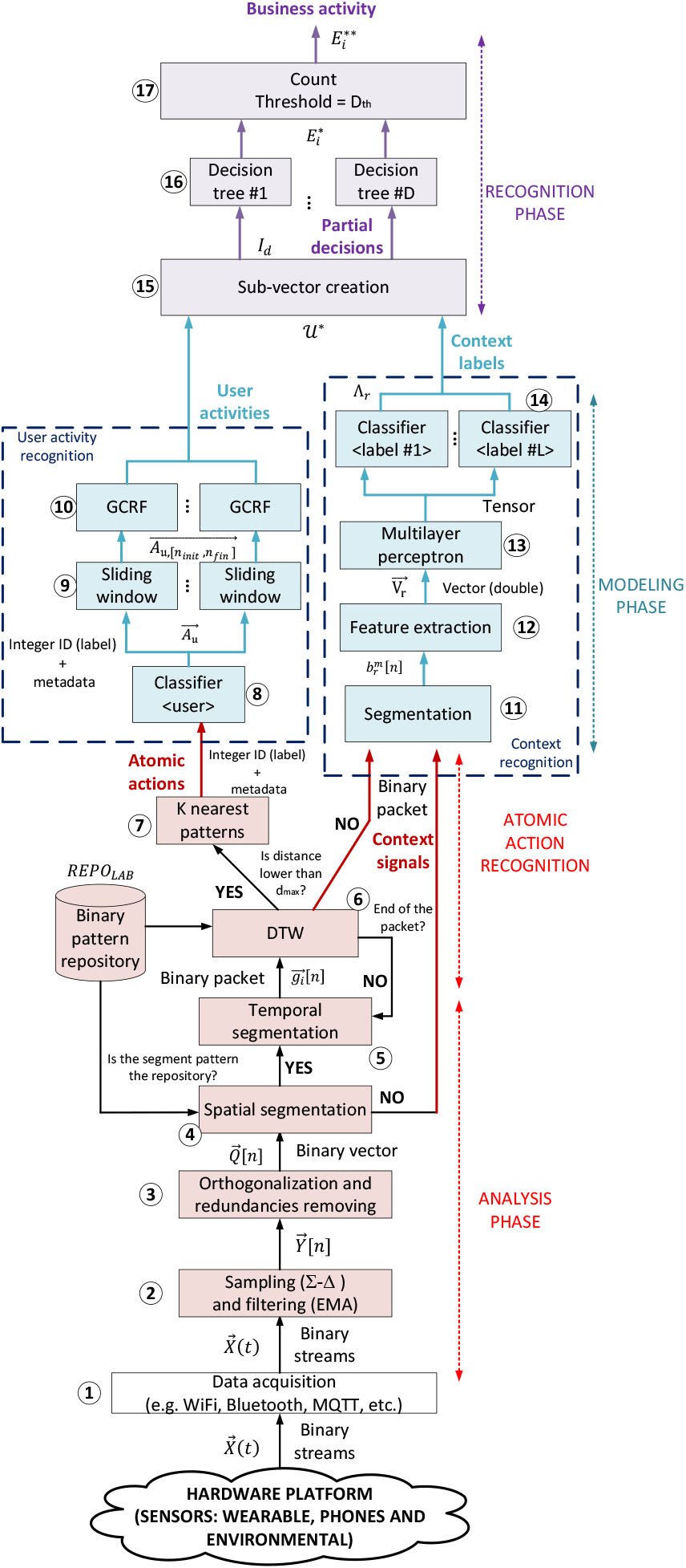
In this paper we propose a hybrid approach in three steps. The first step (analysis phase) analyzes heterogenous signals from different sensor types, and recognizes atomic actions limited in time and space through the location of emerging patterns. The second step considers the recognized atomic actions to model industrial activities using general CRF (GCRF). This model, however, is focused on actions performed by one person (user activities). In the third step, in order to recognize business activities (performed by several people, for example), all user activities are introduced in a high-precision classifier (random forest), where information (labels) about the physical context (extracted from sensor signals) is also employed.
Before any further explanations, some formal definitions must be considered:
• Atomic action: Elemental movement, including some instruments or not, with an objective in the context of the production process (e.g., press a button).
• User action: Independent activity performed by only one worker, which meets a production objective (e.g., controlling a machine).
• Context label: Any representation of the environmental situation in an industrial scenario (e.g., temperature, noise level, etc.).
• Business action: Production activity, which meets an objective at business level (e.g., manufacturing a product).
The proposed solution is supported by pervasive sensing and computing platforms, composed of heterogenous devices with very different behavior and characteristics. Signals are, then acquired through a set of different technologies such as WiFi or publication/subscription brokers [baseline=(char.base)] Â Â Â Â Â Â Â Â Â Â Â [shape=circle,draw,inner sep=0.002pt] (char) 1;. These signals are unsynchronized and multimodal, so an analysis phase is carried out. The analysis phase starts with a noise reduction filter and a digitalization step [baseline=(char.base)] Â Â Â Â Â Â Â Â Â Â Â [shape=circle,draw,inner sep=0.002pt] (char) 2;, based on an exponential mobile average (EMA) and the
These digital signals are then grouped considering spatial restrictions and signal segments are created [baseline=(char.base)] Â Â Â Â Â Â Â Â Â Â Â [shape=circle,draw,inner sep=0.002pt] (char) 4;. If the segment matches the format of any of the patterns in the atomic task repository, the activity recognition process starts. On the contrary, segments are considered context information and sent to the next phase. The atomic recognition process starts with a temporal segmentation [baseline=(char.base)] Â Â Â Â Â Â Â Â Â Â Â [shape=circle,draw,inner sep=0.002pt] (char) 5;, considering the typical duration of activities in the pattern repository. Temporal segments are dynamically calculated through sliding windows. For each possible temporal segment, a Dynamic Time Warping (DTW) algorithm is employed to measure the distance between the segment and patterns in the repository [baseline=(char.base)] Â Â Â Â Â Â Â Â Â Â Â [shape=circle,draw,inner sep=0.002pt] (char) 6;. If that distance is lower than a minimum, the segment is close enough to run the recognition algorithm. On the contrary, the temporal segmentation process in updated and a new DTW distance is calculated. If the binary packet (spatial segment) finishes and the recognition algorithm could not be triggered, the segment is considered context information. Finally, atomic actions are recognized [baseline=(char.base)] Â Â Â Â Â Â Â Â Â Â Â [shape=circle,draw,inner sep=0.002pt] (char) 7;. This algorithm is based on the k-nearest neighbors (K-NN) solution but adapted to future Industry 4.0 scenarios. Recognized atomic actions are represented as labels (integer numbers) with some additional metadata such as the timestamp.
In a craft pottery industry, atomic actions could be, for example, press the pedal of the potter’s wheel or turning it on (if electrical).
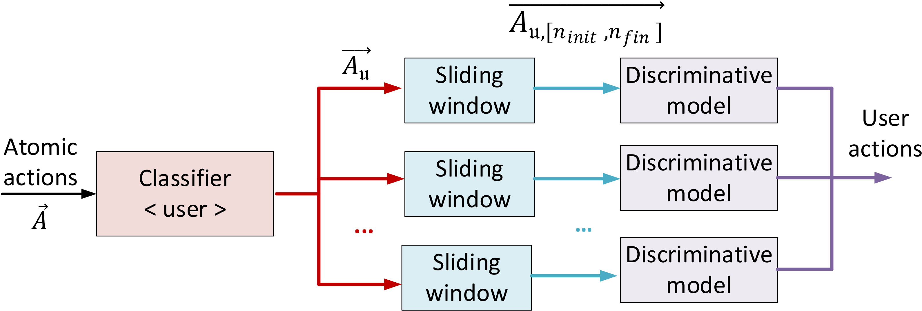
In the modeling phase, two modules are working in parallel: the user activity recognition and the context recognition modules. On the one hand, atomic actions are first classified according to the user performing those actions [baseline=(char.base)] Â Â Â Â Â Â Â Â Â Â Â [shape=circle,draw,inner sep=0.002pt] (char) 8; (using the metadata). Actually, in this modeling phase, we are focusing on activities performed by only one user. Then, each sequence of atomic actions performed by each user is processed using a sliding window [baseline=(char.base)] Â Â Â Â Â Â Â Â Â Â Â [shape=circle,draw,inner sep=0.002pt] (char) 9; to deal with unsynchronicities among users. Different start points are then considered, and all the potential sequences of atomic actions are introduced in a GCRF model. In this module [baseline=(char.base)] Â Â Â Â Â Â Â Â Â Â Â [shape=circle,draw,inner sep=0.002pt] (char) 10;, finally, probabilistic numerical models are employed to determine if some known user actions are recognized. User actions are represented as ASCII labels, typically composed of four or five printable characters (for example, WLK for “walking”). In the same craft pottery industry, an example of user action could be modeling one piece in the potter’s wheel (which includes atomic actions such as press the pedal periodically, move the hands, etc.).
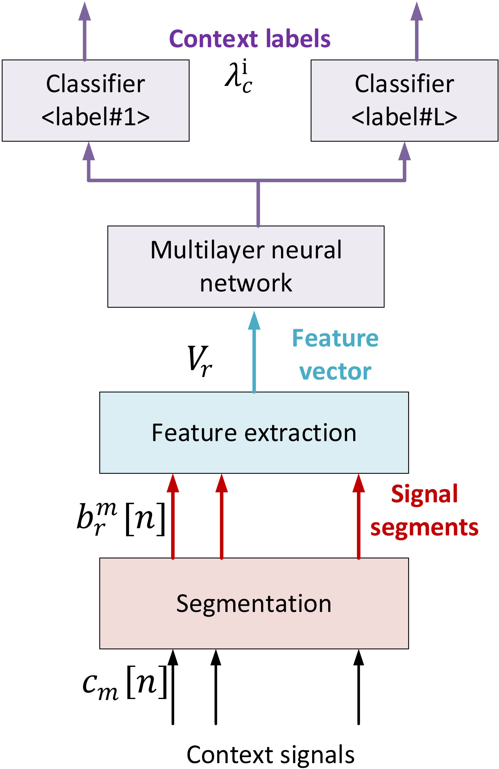
On the other hand, context signals are also processed using a temporal segmentation algorithm [baseline=(char.base)] Â Â Â Â Â Â Â Â Â Â Â [shape=circle,draw,inner sep=0.002pt] (char) 11;, but in this case it is based on a fixed square window. From each segment, then, a set of statistical features [baseline=(char.base)] Â Â Â Â Â Â Â Â Â Â Â [shape=circle,draw,inner sep=0.002pt] (char) 12; (mean, deviation, etc.) are extracted in the next step. These features (as a numerical vector of double precision variables) are then introduced in a multilayer perceptron [baseline=(char.base)] Â Â Â Â Â Â Â Â Â Â Â [shape=circle,draw,inner sep=0.002pt] (char) 13;. Specifically, this context recognition module is based on a supervised learning algorithm, built as a neural network. This perceptron generates a tensor (matrix with double values) which feed a set of classifiers [baseline=(char.base)] Â Â Â Â Â Â Â Â Â Â Â [shape=circle,draw,inner sep=0.002pt] (char) 14;. Context labels are attributes (key-value pairs) indicating the temperature, geographical position, etc.
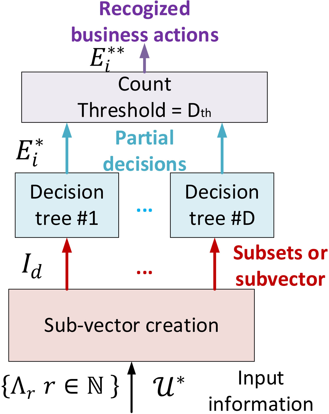
Finally, all user actions and context labels are finally combined to recognize the high-level business actions. A random forest approach is employed. First [baseline=(char.base)] Â Â Â Â Â Â Â Â Â Â Â [shape=circle,draw,inner sep=0.002pt] (char) 15; both inputs are combined to create vectors containing a list of user actions and the corresponding context label as well. With this vector a new set of classifiers, in this case, decision trees, are fed so each tree evaluates [baseline=(char.base)] Â Â Â Â Â Â Â Â Â Â Â [shape=circle,draw,inner sep=0.002pt] (char) 16; which business action is being performed independently. A counter selects [baseline=(char.base)] Â Â Â Â Â Â Â Â Â Â Â [shape=circle,draw,inner sep=0.002pt] (char) 17; the most recognized activity by the decision trees as the final recognized business action. In general, business actions may be represented employing any data format, required by the visualization dashboard or management platform. For example, YAWL or simple ASCII labels. Many different examples of business actions could be imagined. For example, product production in a craft pottery industry (that includes, design, modeling, decorating, etc.)
In general, as previously proposed in other very precise hybrid approaches [40], recognition and analysis technologies in the lower levels (DTW, KNN) are noise-tolerant although less precise than other alternatives. And, in the higher layers, very precise solutions are proposed taking profit of the noise removing and data curation in the lower layers.
Next subsections are describing all details about each one of these three phases.
3.1Analysis phase
In an Industry 4.0 scenario we are considering a pervasive hardware platform composed of
Thus, after acquiring and aggregating all information sources, we obtain a time-variant vector
(1)
First, in the general case,
(2)
The sampling period
(3)
This frequency may be modified according to the scenario and the considered hardware devices (for example, if cameras are also employed), but is adequate for environmental sensors, wearables and smartphones.
Considering this very reduced bandwidth, and the extremely high resolution required to maximize the precision of the following recognition algorithms, the sampling and retention scheme we are employing is a sigma-delta encoder. Figure 2 describes the block diagram of a standard
Figure 2.
Basic block diagram for a
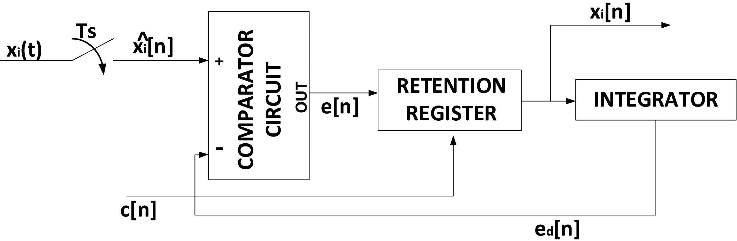
Now, this initial digital vector, in general, is affected by physical random phenomena such as electronic noise, interferences, etc. These high frequency components may affect the following steps, so they must be removed. To do that, an exponential smoothing filter or exponential moving average (EMA) has been proved to be the most effective technique with time series. However, people tend to evolve with the workday, what creates trends in signals which may be removed by EMA. Besides, these trends are seasonal, as they are repeated every day. Because of these characteristics, we are not employing a simple EMA but a triple exponential smoothing (or Holt-Winters method), consisting of three EMA applied in a recursive manner. The first EMA applies an overall smoothing Eq. (3.1). The second EMA preserves the trends in signals Eq. (3.1). And the third and final EMA must preserve the seasonal information Eq. (6). The smoothed time series
(4)
(5)
(6)
Now, in the smoothed vector of time series
• Physical constraints: They are due to physical laws. For example, two close ambient sensors should generate the same output.
• Design constraints: They are due to the selected technological architecture. For example, two digital sensors are programmed to generate reversed bits.
• Business constraints: These constraints are caused by mandatory business workflows and routines in the industrial scenario.
These constraints, in industrial scenarios, are typically scleronomic (i.e. they are independent from time); and besides they are holonomic (i.e. they are independent from differential operations on the coordinates). In those conditions, constraints may be expressed as simple functions Eq. (7). These functions may be employed to remove redundant components in the smoothed vector
(7)
(8)
In general, this new vector will have
3.2 Atomic action recognition
In this context, it is possible to evaluate the similarity of two generalized vectors (or patterns) using simple distance functions, what enables doing a large number of comparisons in a short time (Euclidian distances are extremely computationally low-cost). In that way, the distance between two patterns or generalized vectors
(9)
However, in Industry 4.0 scenarios, atomic actions take a time period to be executed,
(10)
Theoretically, DTW distance could be directly applied to patterns
As said, in this initial analysis phase, atomic actions are recognized. To do that, the
This atomic action recognition process, basically, calculates the distance between elements
The pattern repository
The pattern
(11)
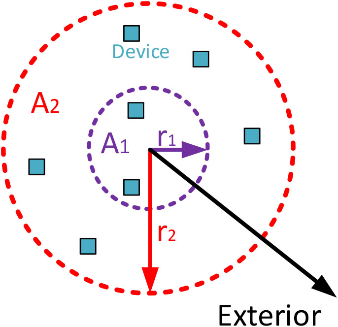
To separate atomic actions, we are grouping components
•
•
Limits for these areas (
Figure 3.
Spatial distribution of information sources.
All possible sets
(12)
Segmenting time series
To perform this action, we are proposing a sliding window scheme. This window
Figure 4.
Sliding window mechanism in the analysis phase.
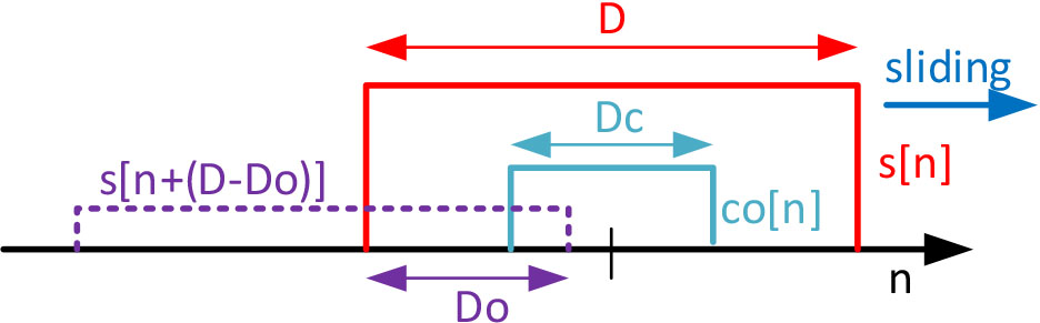
The proposed solution operates in the following manner (see Algorithm 1). The windowed time series (segment) is compared to the patterns (using the proposed DTW technique) considering as initial sample every sample from the initial one to the
| Algorithm 1: Time segmentation of time series |
|---|
| Input Pattern |
| Output Detection of |
| Integer |
| while |
| Calculate |
| Create the final distance between pattern |
| Create the warping path |
| for each value of |
| for each value of |
| Calculate a square window |
| values in samples between |
| Calculate |
| |
| if |
| |
| |
| end if |
| end for |
| end for |
| if |
| return event pattern |
| |
| end if |
| Increment |
| end while |
This sliding window and segmentation process is meant to, mainly, reduce the false negative elements, increasing the system recall. In noiseless scenarios, DTW technologies are tolerant to add or remove several samples from the signals. However, in noisy scenarios as distance thresholds must be more restrictive to avoid false positive elements, the segmentation process is essential to ensure all samples and contributions are considered.
In the most basic approach, the detected atomic actions
(13)
This weighting parameter
(14)
(15)
After recognizing the atomic actions being performed, all components
3.3Modeling phase: User activities recognition
At this point, we have obtained two data structures. On the one hand, a set
In the general case, we are considering
(16)
On the other hand, a set of context signals
(17)
In the modeling phase, these two data structures are employed to evaluate user action and context models. Each one with a different approach (Conditional Random Fields and Neural Networks). As a result, user actions and context labels are recognized.
First, we are discussing how user actions are recognized.
A repository
(18)
As referred for the atomic action repository, in this case the cost of supervising users and creating the repository of user actions is not negligible. Specifically, this cost grows up exponentially with the number of workers and activities under consideration.
Now we are evaluating the conditional probability of a user
(19)
(20)
However, set
Figure 5.
Aggregation process of atomic actions in the modeling phase.
Then,
(21)
Now, atomic actions in each subset
Figure 6.
Sliding window mechanism in the modeling phase.
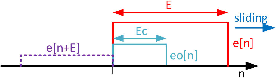
Recognized atomic actions are ordered as a time series, according to their timestamp. Then, a window
(22)
Besides, we are defining a core
The windowed (aggregated) atomic actions
| Algorithm 2: User action recognition process |
|---|
| Input Recognized atomic actions |
| Output Recognized user actions |
| Create variable |
| while |
| Read label |
| Store |
| for each value of |
| if |
| for each value of |
| Select the first k atomic actions in |
| and store them in a set |
| for each user action |
| Estimate the probability |
| if |
| |
| |
| |
| end if |
| end for |
| end if |
| Remove all atomic actions in |
| Return |
| end for |
| end while |
At this point, we only must discuss how the conditional probability
Each one of the random variables considered in the conditional probability (
(23)
In real Industry 4.0 scenarios, despite the variable and flexible character of activities, actions tend to be performed following a minimum common structure (according to the production process, for example). Thus, once a certain atomic action
In those conditions, it is possible to develop the conditional probability as a product or partial probabilities (one for each atomic action
(24)
At this point, in order to improve the precision of the model, we can add (artificially) information about previously recognized user actions, contained in the set
(25)
Each elemental probability
(26)
Now, as humans might freely perform any action at any time, function
(27)
(28)
On the other hand, as function
(29)
Each, factor, as said before Eq. (3.3) may be expressed as an exponential function considering an energy function. Thus, it is induced a new factorization Eq. (30).
(30)
Now, we can rewrite the expression for the conditional probability considering the GFR Eqs (3.3) and (3.3).
(31)
Functions
(32)
(33)
Functions
(34)
(35)
Parameters
(36)
In our approach, we are not using a generic model, but a model that is adapted to the industrial scenarios since the beginning and the initial mathematical definition. That is a novelty compared to existing solutions, which causes a relevant increase in the system precision and justifies the higher processing delay.
3.4 Modeling phase: Context label recognition
Now, we are paying attention to the context signals Eq. (3.3), which must be transformed into high-level context labels in this phase (to enable the business action recognition process in the final phase).
In this case, context series do not represent a behavior as complex as human behavior (like atomic actions), but the evolution of the environment (which is, in general, much slower, and predictable). Thus, a more standard approach may be employed to create context labels from these context signals.
Figure 7.
Implementation of the context recognition module.
First, we are defining a set
(37)
Table 2
Features extracted from context signal segments
| Feature | Mathematical expression |
|---|---|
| Maximum value |
|
| Minimum value |
|
| First maximum |
|
| First minimum |
|
|
| |
|
| |
|
| |
| Median |
|
|
| |
| Entropy |
|
| Mean of gradient signal |
|
| Mean of Laplacian signal |
|
In the proposed context recognition module, we are first segmenting context signals
(38)
(39)
(40)
Then, for each position of the sliding windows we are obtaining a large vector
(41)
Figure 8.
Proposed architecture for the multilayer perceptron.
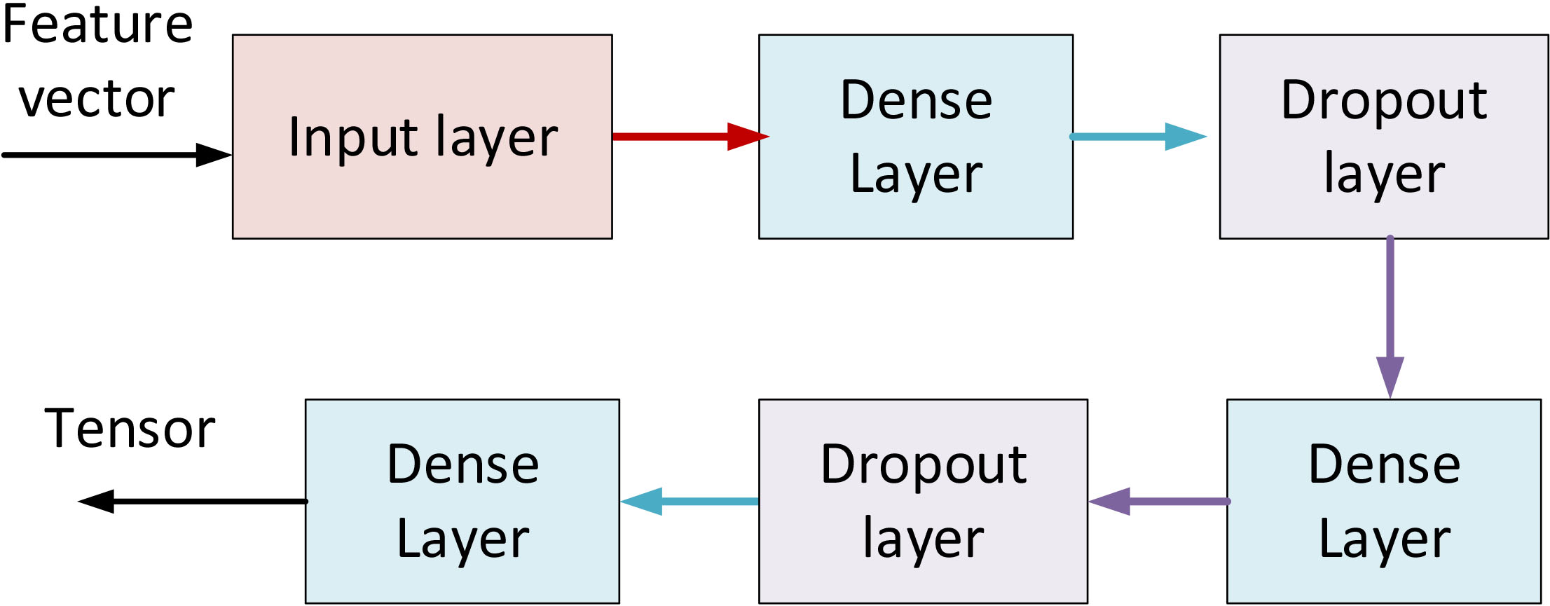
This vector becomes the input of a neural network. For this neural network, we propose a multilayer network, specifically a Multilayer Perceptron (MLP) formed by a stack of five hidden layers (see Fig. 8). There are two dense layers followed by Dropout layers with a rate of
For the training process, we use a stochastic gradient descent algorithm and Adam optimization (considered to be the fastest to converge) with a small learning rate of
We chose this architecture for its simplicity, computational efficiency and flexibility, which allow us to reach the real-time requirements of Industry 4.0 scenarios. As in the user activity recognition module, this neural network must be trained to capture information about the application scenario. To perform this process, we are also employing standard instruments.
Finally, after the classification process, we obtain for each time instant (position of the sliding window) a set
3.5 Recognition phase
For this final phase, we need a new classification technique being able to chop input information and analyze the parts independently, although partial results must be later composed to obtain a global result. This description perfectly fits with a classifier based on Random Forests [37].
Random Forest technique consists of a set of
(42)
Each tree, then, evaluates the input subset (or sub-vector) and decides about which business action
(43)
Figure 9.
Proposed architecture for the random forest classifier.
This repository, as the other ones described in this paper, is created by supervising users and workers in the scenario under study for a period. All repositories may be created at the same time through a unique configuration phase. Atomic, user and business actions and activities should be defined by managers or industry experts according to the production processes, manufactured products, and business objectives. Any modeling language could be employed for this purpose.
Besides, we are modifying classic Random Forest; and all business actions
4.Evaluation and discussion
In order to evaluate the performance of the proposed solution, in this section we carry out a set of relevant experiments and provide and analyze the obtained results.
4.1Experimental validation: Materials and methods
To evaluate the performance of the proposed technology, two experiments are planned and performed. The first experiment was focused on evaluating the quality of the described technique through a set of standard indicators in the field of activity recognition solutions. The second experiment was planned to evaluate the performance of the new technology in terms of execution time and scalability. To perform these studies, the new activity recognition mechanism was implemented and executed using MATLAB 2017 software suite. In order to guarantee the obtained results for the new technology during the planned experiments are comparable to results previously reported in the state of the art, we are basing both experiments in standard datasets commonly employed to evaluate activity recognition technologies. Specifically, we have selected two different datasets: ExtraSensory [23] dataset and UJAmI dataset [16].
ExtraSensory dataset contains, mainly, information provided by personal mobile sensors integrated into mobile phones. Sensors such as accelerometers, gyroscopes and magnetometers are included in this dataset. On the other hand, UJAmI dataset contains information from a pervasive hardware platform including sensors such as NFC tags or temperature and CO2 sensors. Besides, to guarantee the statistical significance and validity of the results, the performance of the new activity recognition technology is analyzed through a
Datasets employed in these experiments were selected according to different criteria:
• Datasets must contain information about unconstrained activities. Contrary to other applications in real scenarios where people act freely.
• Different users must be present in the dataset. To represent a real Industry 4.0 scenario, more than one worker must be performing activities. This condition also allows us to guarantee the proposed solution generalizes all human-dependent factors in business activities.
• Samples in datasets must be collected according to communication and sampling schemes described in the proposed architecture.
• Information about activities being executed in parallel, with interruptions, and about activities executed by different users in a collaborative manner must be also present in the selected datasets.
• More than one sensor must be present. Preferably, an heterogenous set of information sources must be represented in the dataset.
• Time, context and geographical information must be present in the dataset, to be adequate for the proposed new technology.
With these criteria, two datasets were selected. ExtraSensory dataset describes sixty (60) users performing up to one hundred and sixteen (116) different activities in a multi-tasking scheme. More than 300.000 minutes of monitoring are present in the dataset. Personal mobile sensors are employed. Raw signals are available. On the other hand, UJAmI dataset represents workers performing activities in a pervasive sensing scenario, as it is envisioned to happen in Industry 4.0 applications. Only twenty-four different actions are monitored. Ten days of monitoring are available. UJAmI dataset was initially published in 1996. However, different actualizations and versions have been released and, for this work, we are considering the last 2018 version, so we can guarantee the dataset reflects current Industry 4.0 scenarios.
Table 3
Configuration parameters for the experimental phase
| Parameter | Value | Comments |
|---|---|---|
| Analysis phase | ||
|
| Six hundred and sixty data sources in the ExtraSEnsory dataset (one mobile device per user and eleven sensors per device) | |
| Thirty-nine consolidated data sources in the UJAmI dataset | ||
| B | 12 | Standard number of bits for current analog-to-digital converters |
|
| 80 Hz | Maximum frequency in data signals is 40 Hz |
|
| 0.441 | Traditional values for a standard smoothing effect |
|
| 0.030 | |
|
| 0.002 | |
|
| 6912000 | Season is considered as a workday (24 h) |
|
| Redundant sensors are considered equal | |
| Modeling phase | ||
|
| 80% of available instances in each experiment (depends on the experiment, but around forty thousands) | |
|
| 164 | ExtraSensory dataset provides 116 different activities and UJAmI dataset provides 48 different activities |
| Number of users | 60 | As indicated in the considered datasets |
| Recognition phase | ||
|
| 75 | ExtraSensory dataset provides 51 different activities and UJAmI dataset provides 24 different activities |
|
| 48000 | The maximum variation period for context signals is fixed to ten minutes |
|
| 100 | Default value for a good quality classifier, as reported in the literature |
In order to guarantee that obtained results are not user-conditioned, when creating the five folds in the validation process independent groups of users were considered. Specifically, 80% of users considered in each experiment were employed to train the model and additional 20% of participants were employed to test the performance. Although this approach may cause overfitting under certain circumstances, in our experiment we saw a very high and constant performance in every k-fold. No subset where this performance is significantly lower has been detected. As a result, we can conclude the generalization capacity of our model is very high.
As said, two different experiments were conducted. For both experiments, the proposed new activity recognition technique was configured with a particular set of parameters, which are shown in Table 3.
Most of these parameters must be selected according to the activities to be recognized, although parameters related to the smoothing effect have optimum values that have been analyzed and reported in the state of the art [26]. In order to tune activity-dependent parameters, a “silence” detection analysis based on elemental signal processing may be done, so the length and duration of the different activities may be easily identified and calculated. The spectrogram tool is employed for this purpose in this work.
The first experiment was focused on analyzing the recognition and classification capabilities of the proposed technology. To do that, a standard collection of relevant performance indicators was considered (see Table 4). The entire datasets were employed to train and evaluate the proposed technique during this experiment. Three different situations were defined. In the first one, we are only using the ExtraSensory dataset. In the second one, we are only using the UJAmI dataset. And in the third one we are creating a new dataset, obtained by merging ExtraSensory and UJAmI datasets.
Table 4
Performance indicators considered in the first experiment
| Indicator | Expression |
|---|---|
| Precision |
|
| Recall |
|
| F1-Score |
|
| Specificity |
|
| Balance accuracy |
|
| Root mean square error |
|
| Kappa |
|
In Table 4,
In order to highlight the novelty of the proposed solution, and provide a relevant data comparison, the obtained results are statistically compared to the state-of-the-art hybrid mechanisms [40]. For this purpose, we have selected as reference the hybrid technology showing the highest accuracy [40] among all reported solutions in the last five years. Other more recent proposals [22, 50] could be found, but they show a worse performance. Although different tests could be employed, in this experiment we are using the Mann-Whitney U test, as it has been proved to be effective to compare activity recognition solutions. The
On the other hand, the second experiment was focused on the performance and scalability analysis of the proposed technology. Considering the dataset generated by merging ExtraSensory and UJAmI datasets, the required time for the training process and the recognition delay are measured. From this dataset, different folds were extracted containing different numbers of users. For each fold, the training and recognition delay was measured. From this experiment, the required processing time, the scheme scalability and the algorithm temporal order was calculated and discussed.
4.2Results
Table 5 provides the obtained results for the first experiment. Globally, these results are coherent both, internally (among the different indicators) and externally [37]. No dissonant value or result may be seen, so they may be considered valid and statistically representative of the technology’s behavior. This conclusion is also supported by the high values in the Cohen’s kappa score. From Table 5 it can be deducted the proposed mechanism present a very good behavior as activity recognition technique in Industry 4.0 scenarios: F1-Score is near 0.9 for all experiments (even significantly above this value for the UJAmI dataset).
Table 5
Results from first experiment
| Indicator | ExtraSensory | UJAmI | ExtraSensory |
|---|---|---|---|
| Precision | 0.869 | 0.957 | 0.859 |
| Recall | 0.875 | 0.960 | 0.870 |
| F1-Score | 0.872 | 0.959 | 0.864 |
| Specificity | 0.879 | 0.965 | 0.880 |
| Balance accuracy | 0.877 | 0.963 | 0.875 |
| Root mean square error | 0.105 | 0.089 | 0.109 |
| Kappa | 0.904 | 0.923 | 0.903 |
In crowdsensing scenarios (represented by ExtraSensory dataset), precision is almost 87%. This value considers all business activities represented in the ExtraSensory dataset together (such as driving, cooking, or working in the lab). Activities are heterogenous enough to represent a large catalogue of potential Industry 4.0 scenarios. The same catalogue of activities has been previously recognized using other approaches, some of them even similar to the proposed solution, and obtained results with our proposal (globally) improve up to 10% the performance of these state-of-the-art techniques [37] applied to the same dataset. In general, activities that are performed in a continuous and homogeneous manner (such driving or walking) are recognized with a better precision than activities that are non-continuous (such as cooking or bathing). The difference in precision between both kinds of activities is around 2.5%.
The best results are obtained for UJAmI dataset, which represents environments based on pervasive sensing platforms, and shows a F1-Score around 10% higher than experiments with other datasets. On the other hand, the proposed scheme in this work improves the precision around 8% compared to the state-of-the-art proposals where the entire catalogue of activities in the UJAmI datasets are considered [27].
More complex Industry 4.0 scenario will include both, personal sensors and pervasive sensing platforms. These scenarios are represented by the merged ExtraSensory
Although some discussions have been provided, comparing the results with state-of-the-art mechanisms, Table 6 shows a formal statistical comparison with existing hybrid approaches [40] using the Mann-Whitney U test. As it can be seen, in general for all metrics the proposed solution is significantly better than the state-of-the-art hybrid mechanisms [40] applied to the same datasets.
Table 6
Comparison of different indicators with the state of the art
| Indicator | ExtraSensory | UJAmI | ExtraSensory |
|---|---|---|---|
| Precision | ** | * | * |
| Recall | ** | ** | ** |
| F1-Score | * | ** | NS |
| Specificity | ** | ** | ** |
| Balance accuracy | ** | ** | ** |
| Root mean square error | *** | ** | ** |
| Kappa | * | * | * |
NS not significant;
First, in general, all metrics improve with a significance level of 0.005. However, in our approach, F1-score shows a more similar behavior to previous proposals than other metrics, and the significance level reduced in one magnitude order. Even, for the experiment considering the ExtraSensory and UJAmI datasets together no difference is detected. Any case, globally, we can conclude the proposed scheme improves the performance of state-of-the-art mechanisms, as Kappa parameter shows a relevant improvement with a significance level of
In order to add more information to the discussion, we are analyzing some relevant activity types. Namely, the continuous (C) and non-continuous (NC) activities, and the activities performed by one (I) or by several (G) workers together. These disaggregated results are represented in Fig. 10. Besides, Table 7 present the confusion matrix for these four groups and all the considered datasets.
Figure 10.
Precision, recall and F1-Score for some relevant activity types.
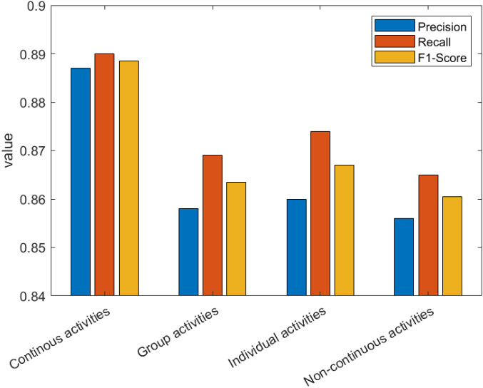
Continuous activities are those that last for a long period generating a homogeneous and almost permanent sensor outputs (such as driving or sitting). On the other hand, non-continuous activities are those that last a short time or have a variable behavior (for example, cooking).
As can be seen there is no big difference between performance for individual and group activities. Indicators are slightly higher for individual activities, but differences are below 1%. Only errors originated in this last phase affect the differences between individual and group activities (contrary to other approaches based on monolithic solutions).
Table 7
Confusion matrix for some relevant activity types
| Dataset | Recognized | |||||
|---|---|---|---|---|---|---|
| NC | C | I | G | |||
| ExtraSensory | Real activity | NC | 0.883 | 0.161 | ||
| C | 0.124 | 0.888 | ||||
| I | 0.897 | 0.155 | ||||
| G | 0.158 | 0.865 | ||||
| UJAmI | NC | 0.906 | 0.103 | |||
| C | 0.071 | 0.917 | ||||
| I | 0.965 | 0.103 | ||||
| G | 0.094 | 0.909 | ||||
| ExtraSensory | NC | 0.896 | 0.148 | |||
| C | 0.114 | 0.877 | ||||
| I | 0.865 | 0.140 | ||||
| G | 0.141 | 0.849 | ||||
Table 8
Comparison of different indicators with the state of the art
| Dataset | Indicator | ||||
|---|---|---|---|---|---|
| Precision | Recall | F1-score | |||
| ExtraSensory | Real activity | NC | * | ** | NS |
| C | ** | ** | * | ||
| I | ** | ** | * | ||
| G | * | ** | NS | ||
| UJAmI | NC | * | ** | ** | |
| C | * | * | ** | ||
| I | * | ** | ** | ||
| G | NS | * | * | ||
| ExtraSensory | NC | * | * | NS | |
| C | ** | ** | * | ||
| I | ** | ** | * | ||
| G | * | * | NS | ||
NS not significant;
However, there is a significant difference (in the environment of 5%) between the performance for continuous and non-continuous activities. In this case, discontinuities affect both, the modeling, and the recognition phases. As a general idea, complex business activities (with discontinuities and several users collaborating together) are recognized with a lower precision (e.g., working in the laboratory) than activities with a simpler structure such as driving or lying.
In order to analyze with more details which kinds of activities are recognized with the best precision, Table 8 shows a statistical comparison of the obtained results with the state of the art, using the Mann-Whitney U test. Besides, in order to enable a heuristic comparison, Table 9 shows the values for the main indicators (precision, recall, specificity and F1-score).
Table 9
Main indicators for the main types of activities
| Indicators | ||||
|---|---|---|---|---|
| Precision | Recall | Specificity | F1-score | |
| NC | 0.896 | 0.858 | 0.884 | 0.878 |
| C | 0.877 | 0.884 | 0.858 | 0.880 |
| I | 0.865 | 0.860 | 0.858 | 0.862 |
| G | 0.849 | 0.858 | 0.860 | 0.853 |
First, in general, all kind of activities shows a significant improvement in all metrics compared to the state of the art. In general, precision and F1-score improvement have a significance level of
Regarding the different activity types, continuous and individual activities (as they have a simpler structure) are recognized with a better precision, recall and F1-Score. This includes activities such as lying, sitting, running or driving. In this case, the significance level of the improvement is close to
Figure 11 shows the results of the second experiment. As can be seen (Fig. 11b), only around 200 milliseconds are required to recognize a business activity using the proposed framework. Almost-random variations may be observed in the figure, of 3% between the maximum and minimum values, but they can be easily explained by exogenous processes affecting the experiment, such as delays caused by the operating system and other applications that are sharing the resources. Any case, seen the obtained graphic, the temporal order of the proposed solution during the operation phase is almost linear with respect to the number of users. This is the most desired behavior for industrial solutions.
Figure 11.
(a) Evolution of the time required in the training process for different numbers of users in the dataset. (b) Operation delay for different numbers of users.
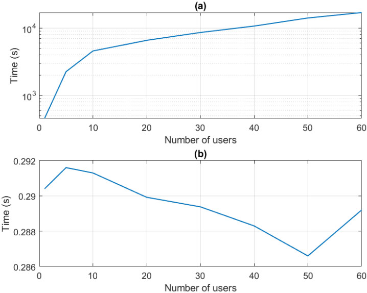
On the other hand, in Fig. 11a the required time for the training process is shown. Values range between only twenty minutes (approximately) for scenarios where only one user is employed to train the algorithm; to around four hours, required in scenarios where sixty workers are involved in the training process. These results are coherent with the idea that training processes in our solution are performed using standard mechanisms, which have showed similar behaviors in other previously reported works [52].
In this case, and using a fitting mechanism, we have found that the temporal order of the proposed solution during the training process is
5. Conclusions
In this paper, it is proposed a new activity recognition technology, focused on Industry 4.0 scenarios. The proposed mechanism consists of different steps, including a first analysis phase where physical signals are processed with DTW technologies; a second phase where activities are modeled using CRF, and neural networks are employed to analyze context information; and a third step where activities are recognized using previously recognized user actions and context information, formatted as labels.
The proposed solution achieves the best recognition rate of 87% which demonstrates the efficacy of the described method. Results show that the proposed mechanism improves up to 10% the precision of previously reported technologies which a relevant significance level, when applied to Industry 4.0 (craft industry) scenarios. On the other hand, the weight of craft industry within the global Industry 4.0 sector may be small (depending on the region, country, etc.), so other less precise mechanisms could be considered in practice by companies, if they are low-cost because of the exponential economy. Solutions such as artificial vision, which is exhaustively employed in other sectors like the automotive sector, but currently have limited applicability in craft industries, could be then deployed in this scenario because of its affordable cost.
Future works will consider the validation of the proposed solution in different Industry 4.0 scenarios. Besides, other classifiers during the recognition may be employed, in order to adapt the proposed mechanism to certain critical scenarios where, for example, only video signals are available (for example, in energy companies). Future works will also analyze how the proposed solution may be applied to other large-scale industries such as the automotive sector.
Acknowledgments
The research leading to these results has received funding from the Spanish Ministry of Science, Innovation and Universities through the COGNOS project (PID2019-105484RB-I00).
References
[1] | Lu Y. Industry 4.0: A survey on technologies, applications and open research issues. Journal of Industrial Information Integration, (2017) ; 6: : 1-10. |
[2] | Bordel B, Alcarria R, Robles T, Martín D. Cyber-physical systems: Extending pervasive sensing from control theory to the Internet of Things. Pervasive and Mobile Computing, (2017) ; 40: : 156-184. |
[3] | Perme, MP, Manevski D. Confidence intervals for the Mann-Whitney test. Statistical Methods in Medical Research, (2019) ; 28: (12): 3755-3768. |
[4] | Bordel B, Alcarria R, de Rivera DS, Robles T. Process execution in Cyber-Physical Systems using cloud and Cyber-Physical Internet services. The Journal of Supercomputing, (2018) ; 74: (8): 4127-4169. |
[5] | Noering FKD, Schroeder Y, Jonas K, Klawonn F. Pattern discovery in time series using autoencoder in comparison to nonlearning approaches. Integrated Computer-Aided Engineering, (2021) ; 28: (3): 235-254. |
[6] | Roda-Sanchez L, Olivares T, Garrido-Hidalgo C, de la Vara JL, Fernández-Caballero A. Human-robot interaction in industry 4.0 based on internet of thing real-time gesture control system. Integrated Computer-Aided Engineering, (2021) ; 28: (2): 159-175. |
[7] | Beddiar DR, Nini B, Sabokrou M, Hadid A. Vision-based human activity recognition: A survey. Multimedia Tools and Applications, (2020) ; 79: (41): 30509-30555. |
[8] | Zhang S, Wei Z, Nie J, Huang L, Wang S, Li Z. A review on human activity recognition using vision-based method. Journal of Healthcare Engineering, (2017) ; 2017: : 3090343. |
[9] | Bordel B, Alcarria R, Martín D, Robles T, de Rivera DS. Self-configuration in humanized cyber-physical systems. Journal of Ambient Intelligence and Humanized Computing, (2017) ; 8: (4): 485-496. |
[10] | Bordel B, Alcarria R, Jara A. Process execution in humanized Cyber-physical systems: Soft processes. In 2017 12th Iberian Conference on Information Systems and Technologies (CISTI), IEEE. June (2017) , pp. 1-7. |
[11] | Sánchez BB, Alcarria R, de Rivera DS, Sánchez-Picot A. Enhancing process control in industry 4.0 scenarios using cyber-physical systems. JoWUA, (2016) ; 7: (4): 41-64. |
[12] | Bordel Sánchez B, Alcarria R, Martín D, Robles T. TF4SM: A framework for developing traceability solutions in small manufacturing companies. Sensors, (2015) ; 15: (11): 29478-29510. |
[13] | Martín D, Bordel B, Alcarria R, Sánchez-Picot Á, de Rivera DS, Robles T. Improving learning tasks for mentally handicapped people using AmI environments based on cyber-physical systems. In International Conference on Ubiquitous Computing and Ambient Intelligence Springer, Cham, Nov. (2016) , pp. 166-177. |
[14] | Bordel B, Alcarria R. Assessment of human motivation through analysis of physiological and emotional signals in Industry 4.0 scenarios. Journal of Ambient Intelligence and Humanized Computing, (2017) ; 1-21. |
[15] | Bordel B, Alcarria R, Sánchez-de-Rivera D. A Two-Phase Algorithm for Recognizing Human Activities in the Context of Industry 4.0 and Human-Driven Processes. In World Conference on Information Systems and Technologies, Springer, Cham, April (2019) , pp. 175-185. |
[16] | Espinilla M, Martínez L, Medina J, Nugent C. The experience of developing the UJAmI Smart lab. IEEE Access, (2018) ; 6: : 34631-34642. |
[17] | Benavoli A, Corani G, Demšar J, Zaffalon M. Time for a change: a tutorial for comparing multiple classifiers through Bayesian analysis. The Journal of Machine Learning Research, (2017) ; 18: (1): 2653-2688. |
[18] | Martín Rico F, Gomez-Donoso F, Escalona F, García Rodríguez J, Cazorla M. Semantic visual recognition in a cognitive architecture for social robots. Integr. Comput. Aided Eng, (2020) ; 27: (3): 301-316. |
[19] | Cai E, Li D, Li H, Xue Z. Self-adapted optimization-based video magnification for revealing subtle changes. Integr. Comput. Aided Eng, (2020) ; 27: (2): 173-193. |
[20] | Wu S, Zhang G, Neri F, Zhu M, Jiang T, Kuhnert KD. A multi-aperture optical flow estimation method for an artificial compound eye. Integrated Computer-Aided Engineering, (2019) ; 26: (2): 139-157. |
[21] | Elliott RJ, Aggoun L, Moore JB. Hidden Markov models: estimation and control. Springer Science & Business Media, (2008) ; 29: . |
[22] | Ullah A, Muhammad K, Ding W, Palade V, Haq IU, Baik SW. Efficient activity recognition using lightweight CNN and DS-GRU network for surveillance applications. Applied Soft Computing, (2021) ; 103: : 107102. |
[23] | Kohavi R. Scaling up the accuracy of naive-bayes classifiers: A decision-tree hybrid. In Kdd, August (1996) ; 96: : 202-207. |
[24] | Jacob PE. Sequential Bayesian inference for implicit hidden Markov models and current limitations. ESAIM: Proceedings and Surveys, (2015) ; 51: : 24-48. |
[25] | Ehatisham-ul-Haq M, Azam MA. Opportunistic sensing for inferring in-the-wild human contexts based on activity pattern recognition using smart computing. Future Generation Computer Systems, (2020) . |
[26] | Nakano M, Takahashi A, Takahashi S. Generalized exponential moving average (EMA) model with particle filtering and anomaly detection. Expert Systems with Applications, (2017) ; 73: : 187-200. |
[27] | Salomón S, Tîrnăucă C. Human activity recognition through weighted finite automata. In Multidisciplinary Digital Publishing Institute Proceedings, (2018) ; 2: (19): 1263. |
[28] | Debes C, Merentitis A, Sukhanov S, Niessen M, Frangiadakis N, Bauer A. Monitoring activities of daily living in smart homes: Understanding human behavior. IEEE Signal Processing Magazine, (2016) ; 33: (2): 81-94. |
[29] | Kabir MH, Hoque MR, Thapa K, Yang SH. Two-layer hidden Markov model for human activity recognition in home environments. International Journal of Distributed Sensor Networks, (2016) ; 12: (1): 4560365. |
[30] | Bakar UABUA, Ghayvat H, Hasanm SF, Mukhopadhyay SC. Activity and anomaly detection in smart home: A survey. In Next Generation Sensors and Systems, Springer, Cham, (2016) , pp. 191-220. |
[31] | Lee YS, Cho SB. Activity recognition using hierarchical hidden markov models on a smartphone with 3D accelerometer. In International Conference on Hybrid Artificial Intelligence Systems, Springer, Berlin, Heidelberg, May (2011) , pp. 460-467. |
[32] | Ronao CA, Cho SB. Recognizing human activities from smartphone sensors using hierarchical continuous hidden Markov models. International Journal of Distributed Sensor Networks, (2017) ; 13: (1): 1550147716683687. |
[33] | Pandey A, Jain A. Comparative analysis of KNN algorithm using various normalization techniques. International Journal of Computer Network and Information Security, (2017) ; 11: (11): 36. |
[34] | Liu AA, Nie WZ, Su YT, Ma L, Hao T, Yang ZX. Coupled hidden conditional random fields for RGB-D human action recognition. Signal Processing, (2015) ; 112: : 74-82. |
[35] | Liu J, Huang M, Zhu X. Recognizing biomedical named entities using skip-chain conditional random fields. In Proceedings of the 2010 Workshop on Biomedical Natural Language Processing, Association for Computational Linguistics, July (2010) , pp. 10-18. |
[36] | Knoch S, Ponpathirkoottam S, Fettke P, Loos P. Technology-enhanced process elicitation of worker activities in manufacturing. In: Business Process Management Workshops, Springer International Publishing, (2018) , pp. 273-284. |
[37] | Vaizman Y, Ellis K, Lanckriet G. Recognizing detailed human context in the wild from smartphones and smartwatches. IEEE Pervasive Computing, (2017) ; 16: (4): 62-74. |
[38] | DiPietro R, Lea C, Malpani A, Ahmidi N, Vedula SS, Lee GI, Lee MR, Hager GD. Recognizing surgical activities with recurrent neural networks. In International Conference on Medical Image Computing and Computer-Assisted Intervention, Springer, Cham, October (2016) , pp. 551-558. |
[39] | Hu DH, Yang Q. CIGAR: Concurrent and interleaving goal and activity recognition. In AAAI, July (2008) ; 8: : 1363-1368. |
[40] | Malazi HT, Davari M. Combining emerging patterns with random forest for complex activity recognition in smart homes. Applied Intelligence, (2018) ; 48: (2): 315-330. |
[41] | García-Borroto M, Martínez-Trinidad JF, Carrasco-Ochoa JA. A survey of emerging patterns for supervised classification. Artificial Intelligence Review, (2014) ; 42: (4): 705-721. |
[42] | Bordel B, Alcarria R, Sanchez de Rivera D, Martín D, Robles T. Fast self-configuration in service-oriented Smart Environments for real-time applications. Journal of Ambient Intelligence and Smart Environments, (2018) ; 10: (2): 143-167. |
[43] | Hassan MM, Huda S, Uddin MZ, Almogren A, Alrubaian M. Human activity recognition from body sensor data using deep learning. Journal of Medical Systems, (2018) ; 42: (6): 1-8. |
[44] | Liu X, Cao J, Yang Y, Jiang S. CPS-based smart warehouse for industry 4.0: A survey of the underlying technologies. Computers, (2018) ; 7: (1): 13. |
[45] | Antar AD, Ahmed M, Ahad MAR. Challenges in sensor-based human activity recognition and a comparative analysis of benchmark datasets: a review. In 2019 Joint 8th International Conference on Informatics, Electronics & Vision (ICIEV) and 2019 3rd International Conference on Imaging, Vision & Pattern Recognition (icIVPR), IEEE, (2019) , pp. 134-139. |
[46] | Reining C, Niemann F, Moya Rueda F, Fink GA, ten Hompel M. Human activity recognition for production and logistics – a systematic literature review. Information, (2019) ; 10: (8): 245. |
[47] | Jalal A, Mahmood M, Hasan AS. Multi-features descriptors for human activity tracking and recognition in Indoor-outdoor environments. In 2019 16th International Bhurban Conference on Applied Sciences and Technology (IBCAST), IEEE, (2019) , pp. 371-376. |
[48] | Penumuru DP, Muthuswamy S, Karumbu P. Identification and classification of materials using machine vision and machine learning in the context of industry 4.0. Journal of Intelligent Manufacturing, (2019) ; 31: : 1-13. |
[49] | Luo H, Xiong C, Fang W, Love PE, Zhang B, Ouyang X. Convolutional neural networks: Computer vision-based workforce activity assessment in construction. Automation in Construction, (2018) ; 94: : 282-289. |
[50] | Li X, He Y, Fioranelli F, Jing X. Semisupervised Human Activity Recognition With Radar Micro-Doppler Signatures. IEEE Transactions on Geoscience and Remote Sensing, (2021) ; 1-12. |
[51] | Ibrahim MS, Mori G. Hierarchical relational networks for group activity recognition and retrieval. In Proceedings of the European Conference on Computer Vision (ECCV), (2018) , pp. 721-736. |
[52] | Guillén MA, Llanes A, Imbernón B, Martínez-España R, Bueno-Crespo A, Cano JC, Cecilia JM. Performance evaluation of edge-computing platforms for the prediction of low temperatures in agriculture using deep learning. The Journal of Supercomputing, (2021) ; 77: : 818-840. |

