the Creative Commons Attribution 4.0 License.
the Creative Commons Attribution 4.0 License.
 | 16 Sep 2021
Ozone profile retrieval from nadir TROPOMI measurements in the UV range
Nora Mettig
Mark Weber
Alexei Rozanov
Carlo Arosio
John P. Burrows
Pepijn Veefkind
Anne M. Thompson
Richard Querel
Thierry Leblanc
Sophie Godin-Beekmann
Rigel Kivi
Matthew B. Tully
The TOPAS (Tikhonov regularised Ozone Profile retrievAl with SCIATRAN) algorithm to retrieve vertical profiles of ozone from space-borne observations in nadir-viewing geometry has been developed at the Institute of Environmental Physics (IUP) of the University of Bremen and applied to the TROPOspheric Monitoring Instrument (TROPOMI) L1B spectral data version 2. Spectral data between 270 and 329 nm are used for the retrieval. A recalibration of the measured radiances is done using ozone profiles from MLS/Aura. Studies with synthetic spectra show that individual profiles in the stratosphere can be retrieved with an uncertainty of about 10 %. In the troposphere, the retrieval errors are larger depending on the a priori profile used. The vertical resolution above 18 km is about 6–10 km, and it degrades to 15–25 km below. The vertical resolution in the troposphere is strongly dependent on the solar zenith angle (SZA). The ozone profiles retrieved from TROPOMI with the TOPAS algorithm were validated using data from ozonesondes and stratospheric ozone lidars. Above 18 km, the comparison with sondes shows excellent agreement within less than ±5 % for all latitudes. The standard deviation of mean differences is about 10 %. Below 18 km, the relative mean deviation in the tropics and northern latitudes is still quite good, remaining within ±20 %. At southern latitudes, larger differences of up to +40 % occur between 10 and 15 km. The standard deviation is about 50 % between 7–18 km and about 25 % below 7 km. The validation of stratospheric ozone profiles with ground-based lidar measurements also shows very good agreement. The relative mean deviation is below ±5 % between 18–45 km, with a standard deviation of 10 %. TOPAS retrieval results for 1 d of TROPOMI observations were compared to ozone profiles from the Microwave Limb Sounder (MLS) on the Aura satellite and the Ozone Mapping and Profiler Suite Limb Profiler (OMPS-LP). The relative mean difference was found to be largely below ±5 % between 20–50 km, except at very high latitudes.
- Article
(8580 KB) -
Supplement
(9063 KB) - BibTeX
- EndNote


Ozone is one of the most important trace gases in the Earth's atmosphere. The stratospheric ozone layer is of particular importance for humans because it protects the biosphere from biologically damaging ultraviolet radiation (UV). Ozone is a harmful gas and a strong oxidant. Consequently, in the troposphere it impacts negatively on human health, ecosystem services, and agriculture. Furthermore, tropospheric ozone is a potent greenhouse gas. Ozone also plays an important role in many aspects of atmospheric chemistry, physics, and dynamics. In the stratosphere, ozone is mainly determined by the Chapman cycle (Chapman, 1930) and catalytic loss cycles (Bates and Nicolet, 1950; Salawitch, 2019). The ozone layer heats the stratosphere and thus leads to a vertical temperature maximum (“inversion layer”). The cooling of the stratosphere by ozone depletion and due to climate change is still a subject of research today. Ozone received much public attention when in the 1980s its enormous reduction was observed during Antarctic spring (Farman et al., 1985). This so-called ozone hole is the result of human-made chlorofluorocarbon compounds and is still part of scientific research today. The recovery of the ozone hole is monitored continuously (World Meteorological Organization, 2018). In order to separate dynamical and chemical effects on ozone that vary with altitude, it is not sufficient to limit measurements to total ozone column amounts. The key to ozone monitoring is the precise measurement of its vertical distribution at high spatial and temporal resolution. Two common and accurate methods to measure ozone profiles are ozonesondes and lidars (light detection and ranging). However, neither technique can provide sufficient spatial and temporal coverage. For this reason, the determination of a global ozone distribution is only possible from satellite data.
In addition to the nadir-viewing geometry used here, the atmosphere can also be scanned using limb and solar (lunar/stellar) occultation viewing. This technique has been used among others by OSIRIS (launched 2001; Llewellyn et al., 1997), SCIAMACHY (launched 2002; Burrows et al., 1995), MLS (launched 2004; Waters et al., 2006), SAGE III (launched in 2001 on Meteor-3M and in 2017 on ISS; Cisewski et al., 2014), and OMPS-LP (launched 2011; Jaross et al., 2014). Ozone profiles from limb and occultation data generally have higher accuracy and a higher vertical resolution than nadir-viewing instruments (Hassler et al., 2014). However, the typical along-track spatial resolution is much higher for nadir instruments (6 to 200 km). There is currently the risk of a gap in limb observations in the future, since only very few new limb missions are being planned, while observation programmes using nadir-viewing satellites extend well into the 2040s (EUMETSAT, 2021).
In 1957 a first theoretical retrieval of vertical profiles of ozone from space using passive remote sounding in the ultraviolet (Singer and Wentworth, 1957) was described. UV radiation has a lower penetration depth into the atmosphere at shorter wavelengths, thus permitting the retrieval of vertical ozone profiles using radiation backscattered from the atmosphere and measured by nadir-viewing satellite instruments. With the launch of NIMBUS 4 in 1970 and the backscatter ultraviolet (BUV) spectrometer instrument on it, the measurement of vertically resolved ozone in the atmosphere from space became possible. Regular and continued daily observations started with the solar backscatter ultraviolet instruments SBUV (1978) and SBUV/2 (since 1985). The SBUV ozone profile retrieval uses up to 12 discrete wavelengths (Bhartia et al., 1996). Beside nadir ozone retrieval using the ultraviolet spectral region, the infrared range is also convenient. Nadir sounding in the thermal infrared has a higher sensitivity to O3 in the upper troposphere and lower stratosphere (Turquety et al., 2002).
The first space-borne measurements of contiguous spectra in the ultraviolet and visible spectral regions at sufficiently high spectral resolution were made by the Global Ozone Monitoring Experiment (GOME) instrument (Burrows et al., 1999). These data were used to retrieve ozone profiles from measurements of GOME (Burrows et al., 1999). Munro et al. (1998) demonstrated that the ozone profiles retrieved using the optimal estimation technique were particularly sensitive to the lower stratosphere and the troposphere. Hoogen et al. (1999) highlighted the need for absolute calibration of the satellite measurements to obtain reliable results from GOME. Hasekamp and Landgraf (2001) chose a slightly different retrieval approach using a Tikhonov regularisation, which employs smoothing constraints, instead of the optimal estimation method, that relies on a priori constraints from an ozone profile climatology. van der A (2002) recalibrated the measured spectra from GOME in order to further improve the GOME ozone profiles. Liu et al. (2005) showed that with an extensive spectral correction and a correction of the wavelength scale, information on tropospheric ozone can be further improved.
With the subsequent instruments SCIAMACHY (2002), OMI (2004), and GOME-2 (2006), the spatial resolution of the measurements was improved. Using the OPERA algorithm, van Peet et al. (2013) were able to determine ozone profiles using data from multiple instruments (GOME and GOME-2) with identical settings to obtain for the first time a merged time series, which required a subsequent correction of calibration offsets and a correction for degradation. Miles et al. (2015) developed a retrieval algorithm for GOME-2, which consists of three steps and aims at an even more accurate determination of tropospheric ozone. In the first step, the stratospheric profile is determined from shorter wavelengths of the Hartley ozone absorption band (266–307 nm), in the second step the surface albedo is retrieved using the radiance at 336 nm, and in the last step, the tropospheric profile is retrieved only from the Huggins ozone band (323–335 nm). For OMI, Liu et al. (2010) showed that ozone retrieval with good accuracy (up to 10 % in the troposphere) is possible after a spectral recalibration of the Level 1 data.
With the launch of Sentinel 5 Precursor (S5P) in October 2017, the TROPOspheric Monitoring Instrument (TROPOMI) is another nadir-viewing spectrometer operating in the UV–Vis and SWIR spectral range. It is a follow-up of OMI and SCIAMACHY. Using TROPOMI data, it is possible to continue time series of past and current instruments into the future. The particular advantage of TROPOMI is its unprecedented spatial resolution of 28.8×5.6 km2 in the UV1 band.
The main objective of this study is the first evaluation of UV radiance data from TROPOMI for the ozone profile retrieval with the TOPAS (Tikhonov regularised Ozone Profile retrievAl with SCIATRAN) approach, which is the successor of the FURM (Full Retrieval Method) algorithm (Hoogen et al., 1999). The latest in-flight analyses showed that a recalibration was necessary, especially in the UV range, which leads to an improved level 1B (L1B) spectral data version to version 2 (Ludewig et al., 2020). Since the determination of ozone profiles requires even higher absolute accuracy of the spectra, additional steps in the calibration correction are needed and are presented in this paper.
In the future, an operational TROPOMI ozone profile L2 product will also be provided by ESA/KNMI (ESA/KNMI, 2021a). Due to the ongoing recalibration, this is currently delayed and is expected to be released after summer 2021. So far, the L1B version 1 TROPOMI data in band 3 (314–340 nm) have been used by Zhao et al. (2020) to determine tropospheric ozone and investigate its changing distribution due to the Covid-19 pandemic. Their profile retrieval was limited to the UV3 band because of larger systematic radiance differences in band UV1 and larger fitting residuals in band UV2. The ozone profiles were derived using optimal estimation, and a soft calibration was applied as well. Due to the narrow spectral window, the vertical resolution of their retrieval is very limited (1.5–2 degrees of freedom).
This paper is structured as follows. Section 2 describes the data used in this paper. The TOPAS retrieval method is described in Sect. 3, and in Sect. 4 the retrieval quality based upon a sensitivity study using synthetic spectra is provided. Section 5 discuss the additional implemented calibration correction. In Sect. 6, the TOPAS ozone profile retrieval is validated with ozonesondes and lidar measurements. First results and a comparison to MLS and OMPS limb measurements are shown in Sect. 7. Finally, a summary is given in Sect. 8.
Beside TROPOMI measurements, which are used to retrieve ozone profiles, data sets from other instruments are used in this study for calibration and validation purposes. In particular, ozone profiles from collocated MLS measurements are used to derive calibration corrections for TROPOMI radiances. In addition, these profiles are exploited, together with OMPS-LP data, for an initial verification of the ozone profiles retrieved from TROPOMI. A more extensive validation is performed using globally distributed ozonesonde and lidar measurements.
2.1 TROPOMI
TROPOMI (TROPOspheric Monitoring Instrument) is a nadir-viewing spectrometer and the only instrument on the Sentinel-5 Precursor (S5P) satellite launched in October 2017. S5P is part of the Copernicus Earth observation programme and is designed to prevent a potential gap in global atmospheric monitoring that could arise between existing missions such as OMI and GOME-2 and the upcoming Sentinel-4 and Sentinel-5 (Fletcher and McMullan, 2016). S5P is in a sun-synchronous orbit with an Equator crossing time of 13:30 local time (LT). TROPOMI consists of four spectrometers in the UV, UVIS, NIR and SWIR spectral range. For the ozone profile retrieval, UV1 and UV2 bands are used. Both are located on the same CCD detector. The wavelength range of UV1 extends from 267 to 300 nm and that of UV2 from 300 to 332 nm. The spectral resolution of both bands is 0.5 nm, and the sampling is 0.065 nm. The high spatial resolution of TROPOMI is worth mentioning. One measurement pixel in the middle of the swath covers 28.8×5.6 km2 (across track × along track) in UV 1 and 3.6×5.6 km2 in UV2. The difference between the two channels comes from the different binning factors that are already applied on board. As the intensity of the measured radiation below 300 nm is much lower, the detector pixels in UV1 have to be binned to get an adequate signal-to-noise ratio (SNR). For the ozone profile retrieval, the sampling of UV1 and UV2 has to be matched. To further improve the SNR in both bands, additional binning is applied before the retrieval.
In the middle of the swath 1 UV1 pixel and 8 UV2 pixels are binned in the across-track direction, while in the along-track direction 8 pixels are binned for both UV1 and UV2. At the far end of the swath, the UV1 pixels have half size in the across-track direction, and therefore 2 UV1 pixels have to be binned here to obtain the same size of the 8 UV2 pixels. That results in a spatial sampling of about 45×45 km2 for all pixels. This additional binning reduces the computation time per satellite orbit.
In this study, we use the L1B product of an updated processor version (version 2.0), which is available from the end of 2019. Details of the pre-launch calibration and of the V2 update can be found in Ludewig et al. (2020). Only the V2 update is of sufficient quality for the ozone profile retrieval. At the moment, only a limited data set of version 2.0 is available. The data have not yet been officially released. Modifications in V2 data are still possible until the official release. Between June 2018 and October 2019, data from 2 weeks every 3 months are processed (all in all around 12 full weeks). TROPOMI, like all instruments of this type, also shows drift and degradation effects in the UV channels. Since the same optical path is used for measuring radiance and solar irradiance, these effects cancel to a large degree in the retrieval using sun-normalised radiances. Remaining uncertainties due to errors or changes in the absolute radiometric calibration need to be corrected for. This calibration correction was performed for UV1 and UV2 bands by comparisons with OMPS solar data. The measured TROPOMI irradiance in the wavelength range between 270 and 332 nm is between 5 % and 15 % lower and was corrected by these values in version 2 of the L1B product (Ludewig et al., 2020).
For the ozone profile retrieval, all ground pixels are used which do not have an error flag above 15 for “measurement_quality” or a “ground_pixel_quality” flag greater than 32. The meaning of the flag values is described in the S5P Level 1B data documentation (Kleipool, 2018). In this study, pixels with error flags like “sun glint possible” or “South Atlantic Anomaly” are included. Besides the measured radiance and irradiance, the signal-to-noise ratios contained in the L1B product are used. Here, only single pixels which have a mean SNR(UV1) >20 or SNR(UV2) >50 are accepted. These low SNR limits of the single pixels are then increased by binning (with n pixels) as described above. A Gaussian approach is used for the increasing binning factor: .
2.2 MLS
MLS is a forward-looking microwave limb sounder aboard Aura that was launched in July 2004. It measures millimetre and submillimetre emissions using seven radiometers which cover a spectral region between 118 GHz and 2.5 THz (Waters et al., 2006). Aura is moving on a sun-synchronous orbit with an equatorial passing time of 13:45 LT. MLS has a spatial sampling of ∼6 km across track and ∼200 km along track. Although TROPOMI and MLS do not operate on the same satellite, their measurements are quite close. The maximum distance between the closest MLS and TROPOMI pixels is 1000 km and 1.5 h.
MLS is an extensively characterised and validated instrument measuring among others vertical ozone profiles (Froidevaux et al., 2008; Livesey et al., 2008). The temporal stability was also shown by comparison with, for example, lidar measurements (Nair et al., 2012). The approved vertical range in which the ozone profiles may be used is between 9 and 75 km. The vertical resolution varies from 2.5 to 3.5 km from the upper troposphere to the middle mesosphere. The precision is estimated to be 5 %–100 % at 9–20 km, 2 %–4 % at 20–45 km, and 7 %–30 % at 45–60 km (Livesey et al., 2020). The accuracy varies from 7 % to 10 % in the troposphere and is around 5 % in the stratosphere. The level 2 product version 4.23, which we use, differs very little from the previous versions, especially in the stratosphere.
2.3 OMPS
Another data set suitable for comparison with TOPAS ozone profiles is provided by the Ozone Mapping and Profiler Suite (OMPS) that was launched on board of the Soumi National Polar-orbiting Partnership (SNPP) at the end of 2011. SNPP has a sun-synchronous orbit with the ascending node at 13:30 LT. That means TROPOMI and OMPS operate in a loose formation at a distance of less than 5 min. The measurements used for the ozone profiles retrieval are taken from the limb profiler (LP) and have been available since 2012 (Flynn et al., 2014).
We compare the ozone profiles from TOPAS retrieval with the OMPS-LP profiles retrieved at IUP Bremen by Arosio et al. (2018). The vertical resolution of the OMPS-LP ozone profiles varies from 1.5 to 4.5 km. The retrieval error resulting from the measurement noise is 1 %–4 % above 25 km increasing up to 10 %–30 % in the upper troposphere. The accuracy varies from 5 %–10 % in the whole altitude range, except in the lower tropical stratosphere where a bias of 10 % with respect to ozonesondes is observed.
2.4 Ozonesondes
Balloon-borne ozonesondes provide a well-established data set of in situ measured ozone profiles in the troposphere and lower stratosphere. Ozonesondes can be operated up to an altitude of approximately 35 km and have a vertical resolution of 100–150 m depending on the design and environmental conditions. The measurement precision is 3 %–5 %, and the accuracy is 5 %–10 % (Deshler et al., 2008; Johnson, 2002; Smit et al., 2007). Ozonesondes have been used in many studies on tropospheric and stratospheric ozone and especially for the validation of satellite data (e.g. Kroon et al., 2011; Jia et al., 2015; Huang et al., 2017; Hubert et al., 2020).
The ozonesondes' data for the validation come from the World Ozone and Ultraviolet Radiation Data Center (WOUDC) (WOUDC Ozonesonde Monitoring Community et al., 2021) and the Southern Hemisphere Additional Ozonesondes (SHADOZ) (Witte et al., 2017, 2018; Thompson et al., 2017; Sterling et al., 2018). During the validation period (June 2018 to October 2019) data from 26 WOUDC and 9 SHADOZ stations were available. The stations are displayed in the map in Fig. 1. The collocation criteria for comparison with TROPOMI are 100 km maximum distance and 24 h maximum time difference. Within the 100 km radius of the ozonesonde site, only the closest pixel in time is taken for the validation. SHADOZ profiles were filtered to exclude data that displayed “dropoffs” larger than 5 % (Stauffer et al., 2020). In total, 231 WOUDC and 22 SHADOZ sonde profiles were compared with TROPOMI ozone profiles.
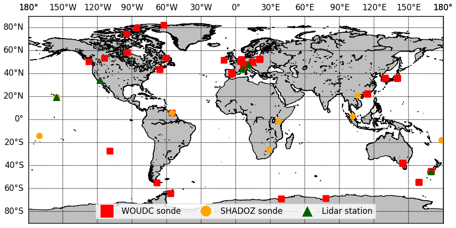
Figure 1Global distribution of ozonesondes (WOUDC and SHADOZ) and lidar measurements used for comparison with the TROPOMI ozone profiles. The exact number and position can be found in Table S1 in the Supplement.
2.5 Ozone lidar
For the validation of ozone profiles, particularly in the upper stratosphere, stratospheric lidar measurements are recommended. The high-power differential absorption lidars (or DIALs) are designed for precise measurements of stratospheric ozone concentration from 20 to 50 km altitude. They use two or more laser wavelengths with strong and weak ozone absorption to measure the backscattered radiation and determine the ozone concentration in the atmospheric layer from their difference. In general, the estimated accuracy of the lidar ozone profiles is 5 % in the 15–50 km range (Leblanc et al., 2016). Like the ozonesondes, lidar measurements are regularly used to validate satellite ozone profiles (e.g. Rozanov et al., 2007; Jiang et al., 2007; Hubert et al., 2016).
For our validation, we used measurements from five lidar stations that are part of the NDACC network (de Mazière et al., 2018). They are marked green in Fig. 1: Hohenpeissenberg (Germany), Lauder (New Zealand), Mauna Loa (Hawaii), Table Mountain (California), and Observatoire de Haute Provence (France). For lidar measurements, we used the same collocation criteria as for ozonesondes and found a total of 177 collocation matches during the validation period.
3.1 Inversion technique
The IUP Bremen retrieval algorithm, which will be referred to as TOPAS, is based on the first-order Tikhonov regularisation approach (Tikhonov, 1963), as described in detail by Rodgers (2002). The relationship between the state vector x that contains the atmospheric quantities to be retrieved and the measurement vector y is given by the forward model operator F(x): , where ϵ represents all errors. For the linearisation of the problem, the derivative K of the forward model is needed, that is called the Jacobian or weighting function matrix:
The linearised expression with the a priori state vector xa is then
The inverse problem is ill-posed and can be solved by minimising the following norm:
Here Sy is the measurement error covariance matrix, and Sr is the regularisation matrix. The latter contains contributions from both the zeroth- and first-order Tikhonov terms, given by
where the zeroth-order Tikhonov term is represented by the a priori covariance matrix, (see, for example, Rodgers, 2002), St is the first-order derivative matrix (see, for example, Rozanov et al., 2011a) and γ a scaling factor.
Since the problem is not linear, an iterative approach is necessary. Here, a Gauss–Newton iteration scheme is used as described in detail by Rodgers (2002). It should be noted that in the first iteration, x0=xa. In the subsequent iterations, x0 is replaced by the solution obtained from the previous iteration, while xa remains fixed. The solution at iteration step i+1 is given by
As in the TOPAS algorithm the relative deviations from the a priori state are retrieved, the appropriate transformation of the state vectors and Jacobian and regularisation matrix is done:
where 1 is the unity vector, and Xa=diag{xa}. Equation (5) is then written as
We note that this transformation also affects the retrieval error matrix, Se, and the averaging kernel matrix, A. The matrices for the transformed variables are related to those for the standard inversion described by Rodgers (2002) as follows:
3.2 Retrieval algorithm
The TOPAS retrieval approach is structured as follows: first, the a priori information in the first iteration or the results from the previous iteration serve as input to the forward simulations with the radiative transfer model (RTM) in the next iteration. A polarisation correction given by a lookup table (LUT) is applied to the simulated intensities and will be described later in this section. In a subsequent preprocessing step, the calibration correction spectrum, the rotational Raman scattering, and an offset correction are fitted to the radiance spectrum and a first-order polynomial is subtracted. Finally, the vertical ozone profile and a Lambertian (scalar) surface albedo are retrieved using Eq. (7). An overview about the relevant retrieval parameters is given in Table 1.
Serdyuchenko et al. (2014)Lamsal et al. (2004)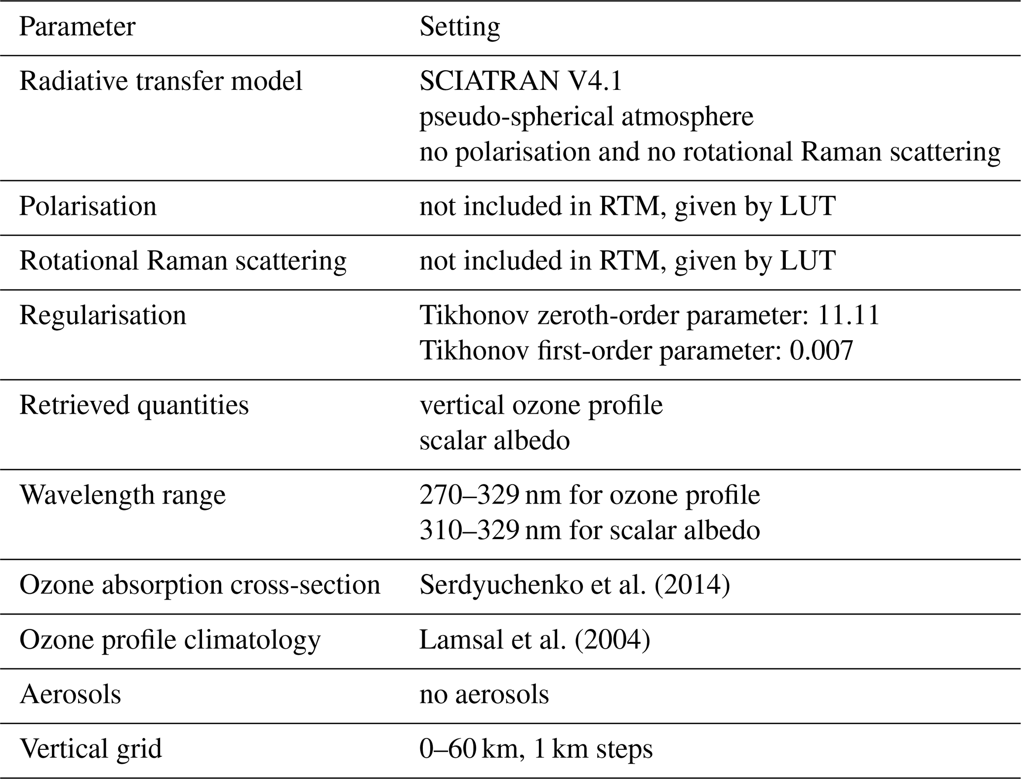
The inversion of the ozone profile is an ill posed mathematical problem. Consequently, the retrieval needs to be constrained by a priori information. Information on total ozone is needed because it helps to determine the ozone profile selected from the climatology as a priori.
The a priori profiles for ozone are taken from the ozone climatology of Lamsal et al. (2004), which contains ozone profiles averaged from sonde and satellite data depending on latitude, season, and total ozone. For each processed profile, the a priori ozone profile is scaled with an initial value for the total ozone. In order to obtain the best possible starting point, the total ozone and the effective scene albedo from the WFDOAS retrieval (Coldewey-Egbers et al., 2005; Weber et al., 2018) applied to TROPOMI is used. For the total ozone amount a positive bias of 2 % in comparison to Brewer and Dobson instruments was found (Orfanoz-Cheuquelaf et al., 2021). Pressure and temperature profiles are taken from the ERA5 reanalysis (Hersbach et al., 2020). The effective scene height accounts for cloud effects and is calculated using surface height, cloud coverage and cloud-top-height. The cloud parameters are part of the operational ESA data product (Loyola et al., 2018). The cloud fraction and cloud-top-height are taken from the offline total ozone S5P product, which contains the OCRA (Optical Cloud Recognition Algorithm) cloud fraction and ROCINN_CRB (Retrieval Of Cloud Information through Neural Networks, cloud as reflecting boundary) cloud altitude matched to the UV3 channel. The cloud-top-height and surface height are weighted according to cloud coverage to determine the effective scene height (Coldewey-Egbers et al., 2005). That enables cloudy and cloudless pixels to be retrieved without a need to account for clouds implicitly in the RTM.
The radiative transfer model SCIATRAN V4.1 is used for the forward simulations (Rozanov et al., 2011a). The radiance in the wavelength range from 270 to 329 nm is simulated with the spectral resolution and sampling of TROPOMI. Polarisation and rotational Raman scattering are omitted for reasons of computing time and are accounted for using a lookup table . Instead of a full-spherical atmosphere, a pseudo-spherical atmosphere is assumed, which accelerates the calculation even more. In this approximation, the direct solar beam is calculated for a fully spherical atmosphere, while for the scattered light, a plane-parallel atmosphere is assumed (Rozanov et al., 2000). This might, however, result in larger errors for larger viewing angles. In this study we use the fact that these errors are largely mitigated if the forward model is run using the angles (viewing, solar zenith, and azimuth) at the surface rather than those at the top of the atmosphere (de Beek et al., 2004).
The radiance spectrum calculated by the RTM is corrected for polarisation using a wavelength-dependent scaling factor. To determine this factor, simulated spectra with and without polarisation are taken from the LUT with appropriate values for albedo, total ozone, geometric height, and viewing geometry. These spectra are then convolved with the TROPOMI instrument response function (ISRF) (ESA/KNMI, 2021b). The ratio of both is then used as a correction factor to account for the polarisation effects.
To account for atmospheric and instrumental effects which are not included in the forward modelling, the preprocessing fit procedure includes three pseudo-absorbers and accounts for a possible misalignment of the wavelength grids of the measured and modelled spectra by performing shift and squeeze correction (Rozanov et al., 2005). During the preprocessing step, the original wavelength range is divided into three spectral windows: 270–300 nm (UV1 for TROPOMI), 300–310 nm (lower UV2) and 310–329 nm (upper UV2). For each of these spectral windows, pseudo-absorbers and shift/squeeze corrections were fitted independently. The first pseudo-absorber used in the fit, which accounts for the missing contribution from the rotational Raman scattering in the forward model, is the Ring spectrum. The Ring spectrum is obtained from LUT using the same procedure as for the polarisation correction spectrum (ratio of convolved radiances modelled with and without rotational Raman scattering contribution). The second pseudo-absorber represents the calibration correction, which accounts for errors in the stray-light correction and other systematic errors in the radiometric calibration parameters. The calibration correction spectrum is determined using the radiances modelled with ozone information from collocated MLS/Aura measurements as described in details below. This pseudo-absorber, as shown in Fig. 5, indicates a discontinuity around 300 nm. In the second spectral window (300–310 nm), the scaling of the recalibration term is not sufficient to remove the discontinuity near the channel boundary. Therefore, in this spectral window, a linear polynomial is fitted by least squares and subtracted for each fitting term separately. The third pseudo-absorber accounts for a wavelength-independent offset in the radiance spectra. To this end, the inverse of the solar spectrum is scaled to the radiance spectra for each of the three spectral windows (Rozanov et al., 2011b).
The Tikhonov regularisation was proven to be very efficient in dealing with non-linear ill-posed problems (e.g. Hasekamp and Landgraf, 2001). The Tikhonov regularisation is particularly effective in smoothing oscillations, which are typical of retrievals at a fine vertical grid.
In the main retrieval step, the first-order Tikhonov regularisation is employed, which ensures that the ozone profile retrieval remains stable and converges, even if the number of independent pieces of information is much lower than the total number of retrieval grid levels. As the zeroth-order Tikhonov term, the inverse a priori covariance matrix, , is used. The a priori variance, which is intended to keep the solution within the natural variability from its a priori value (Rodgers, 2002), is set to 0.3 for both the Lambertian surface albedo and ozone number densities at all altitude levels. The assumed a priori variance for ozone is in generally good agreement with the findings of Lamsal et al. (2004), who reported the variability of ozone to be generally less than 30 % in the upper stratosphere and up to 60 % in the troposphere. In this study, we preferred to use the altitude-independent (constant) a priori variance for ozone rather than the values from the climatology as the latter might introduce vertical irregularity in the retrieval sensitivity, distorting the shape of averaging kernels and occasionally resulting in retrieval artefacts. The strength of the first-order Tikhonov term is controlled by the altitude-independent scaling factor γ (see Eq. 4), which is set to 0.007. The optimum value for this scaling factor is unknown, but through empirical studies we found that this value has the largest information content in the retrieval, and the rms between the measurement and forward model is the smallest. The measurement error covariance matrix, Sy, was filled with squared signal-to-noise ratio (SNR) values, which for the TROPOMI instrument are reported for each spectral measurement in the level 1B product. The noise is a measure for the 1 standard deviation random error of the radiance measurement, and it is assumed to be spectrally uncorrelated; i.e. all off-diagonal elements of the noise covariance matrix are set to zero.
The state vector comprises the ozone number densities at the retrieval grid levels and the effective Lambertian surface albedo. The vertical grid of the retrieval ranges from the effective scene height to the top of the atmosphere (at 60 km) in steps of 1 km. Within each iterative step, the ozone profiles and the effective surface albedo are retrieved independently; i.e. no crosstalk between these parameters is considered. For the ozone profile retrieval, the wavelength range from 270 to 329 nm is used, while the albedo retrieval is done using the 310–329 nm spectral range. A wavelength-independent (constant) surface albedo retrieved from the wavelengths above 310 nm is used in the next iterative step for the entire spectral range. This is done because the radiation at shorter wavelengths barely reaches the ground, and, thus, the surface albedo for wavelengths below 310 nm is much more challenging to determine. We note that the retrieved effective Lambertian surface albedo is not merely the surface reflection but also includes contribution from the backscattering of the radiation by aerosols and clouds. The combined use of the effective scene height and effective albedo eliminates the need to include the contributions from the tropospheric aerosols and clouds in the forward modelling. The iterative process ends when one of the two convergence criteria is fulfilled: the change of the ozone number density in a selected height range or the change of the spectral fit rms (the difference between the measured and modelled radiances) from the corresponding values at the previous iterative step is below 2 %.
4.1 Synthetic retrievals of ozone profiles
One of the widely used approaches to check the self-consistency of the retrieval, investigate its sensitivity, and estimate uncertainties and biases in the retrieved parameters is to undertake sensitivity studies. We call the data sets, used in these sensitivity studies, synthetic retrievals of ozone profiles. To this end, the radiances are simulated using the forward model for a representative set of geophysical scenarios. The retrieval algorithm then runs with the simulated radiances instead of the measured ones. The advantage of this approach it that the true state of the atmosphere is known, which is never the case for the real data.
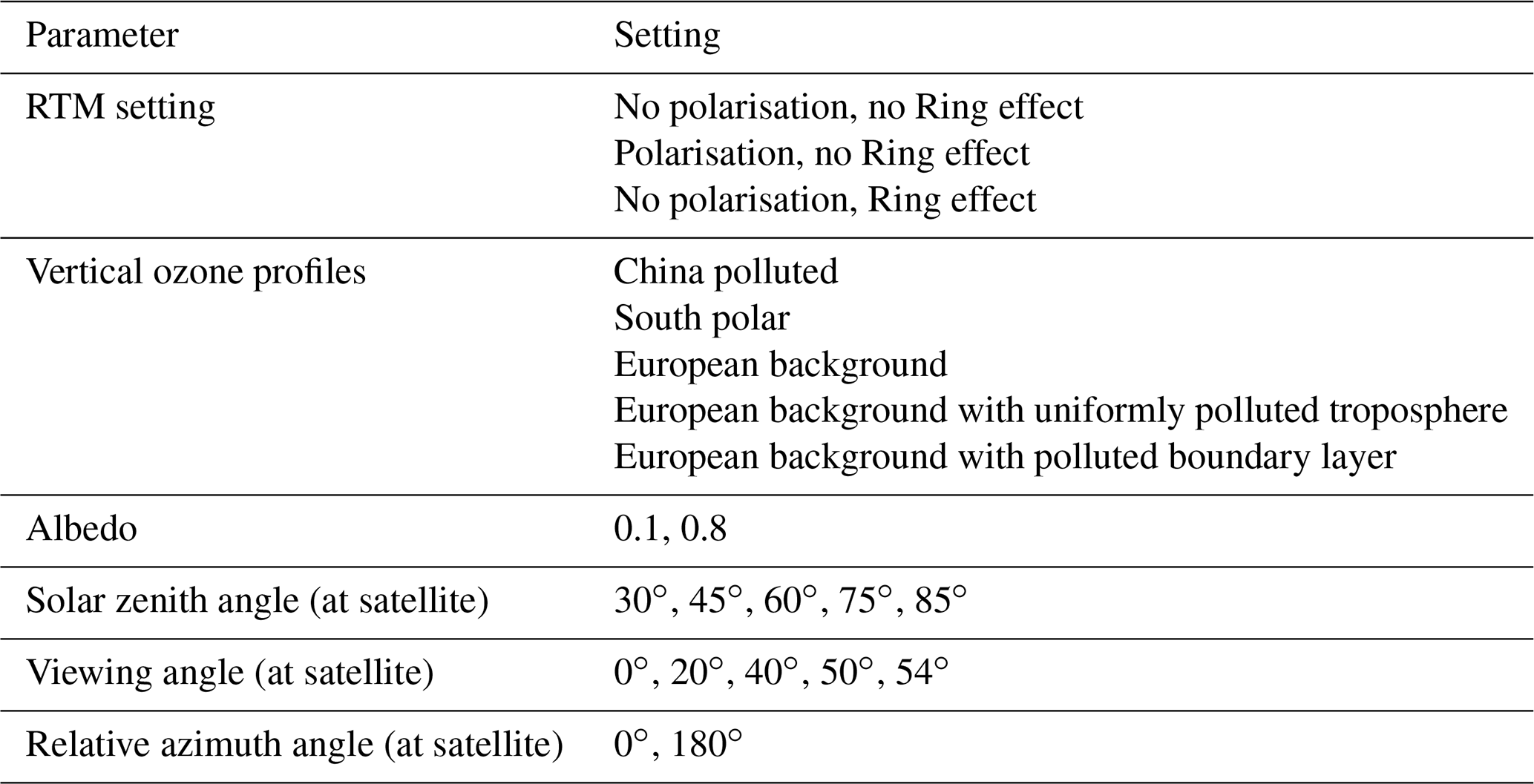
In this study, the radiances are simulated in the spectral range from 270 to 329 nm (TROPOMI UV1 and UV2 bands). The spectral resolution and sampling are set to 0.5 and 0.065 nm, respectively, which is in accordance with the specifications of the TROPOMI instrument. All spectra are simulated assuming a fully spherical atmosphere and multiple scattering. The solar irradiance spectrum from Chance and Kurucz (2010) convolved with the TROPOMI instrument response function is used in the simulations. To investigate the uncertainty associated with the usage of LUTs to account for the polarisation and the rotational Raman scattering (see Figs. S1–S4 in the Supplement), the simulated radiances were calculated with the following settings: (i) without both the Ring effect and polarisation, (ii) with polarisation only (no Ring effect), and (iii) including the Ring effect only (no polarisation). Furthermore, the effect of the viewing and illumination geometry as well as of the surface albedo on the resulting retrieval uncertainties is investigated. The ozone profiles used to calculate the simulated radiances are taken from the CAMELOT study (Levelt and Veefkind, 2009), whose general objective was to establish the quality requirements for air quality and climate monitoring by satellites. Three ozone profile scenarios were selected: European background, China polluted, and south polar. Furthermore, two variants of the European ozone profile with enhanced tropospheric pollution were created: one limited to enhancement in the planetary boundary layer and the other enhanced uniformly over the entire troposphere. The pressure and temperature profiles were also taken from the CAMELOT scenarios. In Table 2, a complete overview of the parameters used in this study is given. In total, 1500 synthetic spectra were generated.
Table 2Input parameters for the generation of synthetic spectra.
The settings for the synthetic retrieval are kept as close as possible to those of the real TROPOMI retrieval. However, a few settings needed to be adjusted. Instead of a measured solar spectrum, we use in the synthetic retrieval the solar spectrum from Chance and Kurucz (2010) convolved with the measured instrument response functions. The signal-to-noise ratio is set in accordance with SNR values extracted from selected TROPOMI measurements. For each scenario, a TROPOMI measurement at possible closest conditions was selected to extract the SNR values. Depending on the wavelengths and viewing and illumination geometry, typical SNR values for binned TROPOMI pixels vary between 100 and 600 in the UV1 band and between 200 and 4000 in the UV2 band. The noise sequences are created with a Gaussian random noise generator available within the SCIATRAN package. For each scenario, 50 independent noise spectra are generated. The synthetic retrievals use the same a priori ozone profiles as for the real TROPOMI retrievals, while the initial guess for the surface albedo is set to a fixed value of 0.5. Since neither calibration errors nor offsets are included in the simulations, and the same RTM is used in the simulation and retrieval, the calibration correction pseudo-absorber is turned off in the synthetic retrievals.
4.2 Sensitivity study
An overview of the ozone profiles resulted from the synthetic retrieval is shown in Fig. 2. The results for the five CAMELOT profile scenarios for all viewing geometry settings and both albedos are shown there. The three European profiles differ only at altitudes below 20 km and are intended to assess the sensitivity of the retrieval to the tropospheric pollution. In the stratosphere, the ozone profile retrieval can reproduce true values very well. For the south polar (panel d) and Chinese profiles (panel e), the a priori profiles deviate from the true values by more than −25 % or up to molec m−3. Despite the large differences between a priori and true profiles, the retrieval results are in a good agreement with the true profiles. The retrieval in the stratosphere seems to be nearly independent of the a priori profile values, as indicated by the measurement response of about 1 (not shown). Since the vertical resolution is limited, a dependence on the shape of the a priori ozone profile remains.
Above 50 km, the sensitivity of the retrieval decreases and the deviations increase. This is explained by the fact that the maximum of the ozone weighting functions at the shortest wavelength lies at about 50 km. Below 25 km, the retrieval results strongly depend on the ozone profile scenario used. In general, the closer the a priori profile is to the true profile, the smaller the retrieval error is. In scenarios with small differences between the a priori and true profiles in the troposphere, the retrieval results seem reasonable. Between 20 and 25 km, all profiles show small negative deviations. Here, the vertical gradient of the ozone profiles is particularly strong, and the retrieval is challenging because the averaging kernels have strong contributions from the ozone peak located above. Below 10 km, the deviations are within 25 % for the European profiles, (panel k) to (panel m), while for the other two profiles, (panel n) and (panel o), the a priori seems to be too far from the truth, so that the retrieval results cannot reach the true values. For the same reason, somewhat larger disagreement between the retrieved and true profiles is observed in the lowermost stratosphere (18 to 25 km).
When the retrieval results are compared to observations or data products having a higher vertical resolution, the latter are usually convolved with the averaging kernels of the former. This also applies to the CAMELOT profiles used here as they have a finer vertical structure than can be resolved by the TOPAS algorithm. The convolution with the averaging kernels is done as follows:
where x and represent the original and the convolved CAMELOT profiles, respectively, xa is the a priori ozone profile, and is the averaging kernel matrix corresponding to the retrieval with the transformed variables (see Eq. 6). In Fig. 2, is shown in green. By applying the averaging kernels, the comparison profiles are smoothed with the strongest changes occurring in the troposphere, where the vertical resolution of the retrieval (as shown in Fig. 3) is lower. The difference between the retrieval results and averaging kernel smoothed comparison profiles is significantly smaller than that without applying the averaging kernels. Overall, the deviations are below ±10 % over the entire altitude range.
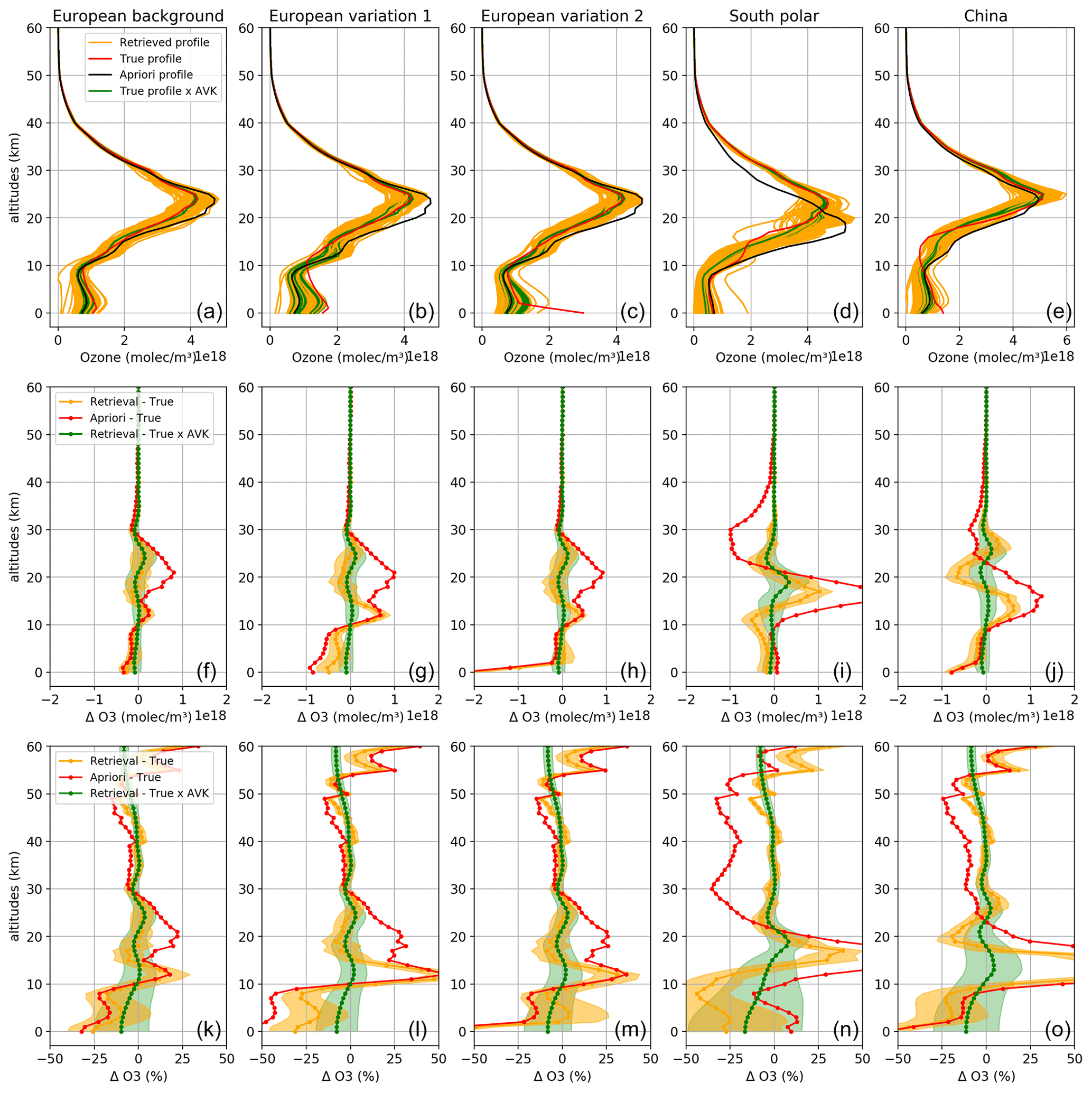
Figure 2Retrieval results for the five CAMELOT scenarios (true); all settings are listed in Table 2. The upper row, (a–e), shows the retrieved (orange), a priori (black), and true profiles (red), as well as the true profiles convolved with the averaging kernels (green). The middle and bottom rows present the absolute (f–j) and percentage (k–o) mean differences between the retrieval results and the true profiles (orange), the mean differences between the retrieval results and true profiles convolved with the averaging kernels (green), and the differences between the a priori and true profiles.
As a next step, we analyse essential retrieval diagnostics, i.e. averaging kernel matrix (AK matrix), vertical resolution, and precision. They are shown for the European background profile (solar zenith angle (SZA) 30∘, viewing angle (VA) 20∘, relative azimuth angle (RAZ) 0∘, albedo: 0.1) in Fig. 3. The averaging kernel matrix consists of 61×61 entries, the averaging kernels (AKs), one for each altitude level. For the sake of clarity, AKs at every 5 km layers are shown in panel (c). At altitudes between 20 and 45 km, the peaks are clearly pronounced and centred at the nominal altitudes of AKs. Above and below this region, the AK shapes are strongly asymmetric. For example, at 15 km there is no clear maximum. At this altitude, the retrieved profile is affected by changes of the true profile in a wide range of altitudes with the strongest contribution from the 12–21 km altitude region and non-negligible influence from altitudes below 25 km to the ground. For the layers below 20 km, a double peak shape of AKs is observed. The averaging kernels for 0 and 5 km do not differ much, which means that no vertical structure can be resolved in the lower troposphere.
The vertical resolution of the retrieval calculated as the inverse of the main diagonal of the AK matrix (Purser and Huang, 1993) is shown in Fig. 3d. The best vertical resolution of about 6 km is reached in the stratosphere between 30–40 km. Above 50 km, the vertical resolution strongly degrades. As a consequence, we perform the TROPOMI retrieval only up to 60 km. In the upper troposphere at about 9 km, the vertical resolution locally degrades to about 20 km and then improves again with the decreasing altitude down to the boundary layer.
Figure 3e illustrates the influence of the measurement noise on the retrieval results. The noise retrieval error calculated in the linear approximation using the Rodgers formalism (Rodgers, 2002; Sect. 3.4.2, Eq. 3.30) is plotted in blue and is around 0.2 %. The error is relatively small because the SNR values from binned TROPOMI pixels are used. In green, the standard deviation of the ozone profiles retrieved from synthetic spectra with different noise sequences added is plotted. It agrees well with the noise retrieval error. Following von Clarmann et al. (2020), we interpret our results as an estimate of the smoothed truth and thus do not consider the smoothing error as an error component.
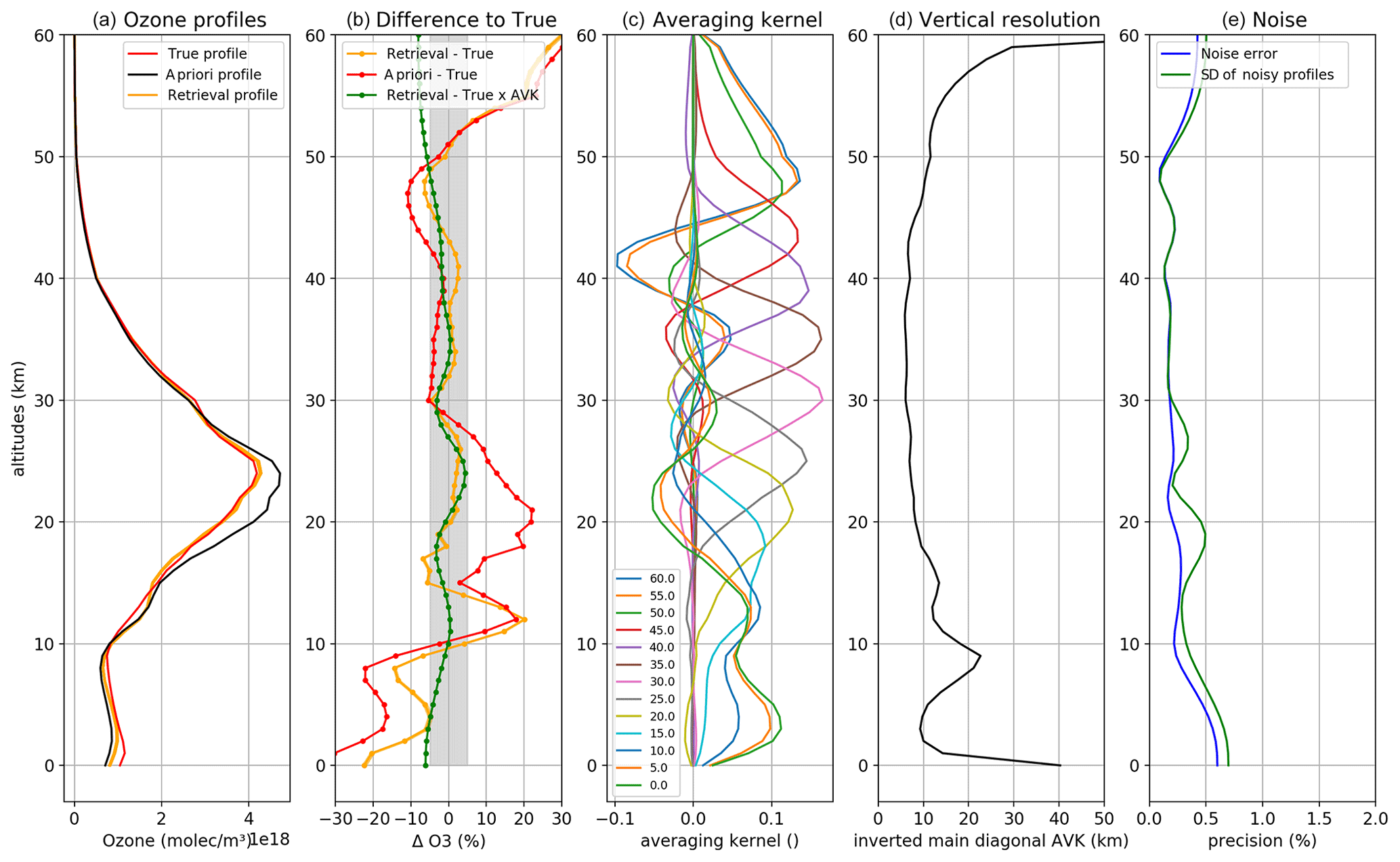
Figure 3Retrieval diagnostics for the European background profile, SZA of 30∘, VA of 0∘, RAZ of 0∘, and albedo of 0.1. (a, b) Profiles and relative mean differences for 50 noisy spectra. (c) Averaging kernels for every 5 km altitude levels. (d) Vertical resolution of the retrieval. (e) Retrieval noise error (blue) as defined by Rodgers (2002) and the standard deviation of the retrieval results from simulated spectra with 50 noise realisations (green).
Figure 4 shows the vertical resolution of the retrieval for all geometries and albedos for one true profile (polluted Chinese case). Each of the four panels shows the results for 25 combinations of the viewing angle (VA) and solar zenith angle (SZA) used in the sensitivity study. On the left, the retrieval results for low surface albedo (0.1) are shown, which simulates cloud and ice-free pixels. On the right, the high-albedo (0.8) scenarios are shown. The top and bottom panels show the vertical resolution of the retrieval for azimuth angles of 0 and 180∘, respectively. Between 18 and 50 km, the vertical resolution is similar for all geometries and surface albedos and ranges from 5 to 10 km. In the troposphere, the vertical resolution degrades to about 15 km (between 1 and 18 km altitude) but improves again in the 5 km altitude region. With exception of the uppermost and lowermost altitudes, the worst retrieval resolution of about 20 km is found at 10 km altitude. Differences between the vertical resolutions for the ground scenes with low and high albedo are most pronounced in the lower troposphere. The best vertical resolution in this altitude range is achieved for high surface albedo and small SZA. It should be noted, however, that a high albedo in the UV spectral range occurs only above clouds or snowy/icy surfaces. Ozone hidden below clouds can of course not be retrieved.
In general, the vertical resolution is determined by the influence of the ozone absorption in each particular altitude region on the total strength of the ozone absorption signal registered by the instrument. Two factors are essential here and both depend on the observation and illumination geometry. These are the length of the effective light path through the altitude layers of interest and the amount of light originating from these layers. While the latter depends on the amount of the incident light and scattering properties of the atmosphere, the light paths always increase with the geometrical angles (SZA, VA, and AA). Furthermore, the simulations were done using TROPOMI-specific SNR values for each viewing geometry, which also influences the sensitivity of the retrieval. The solar zenith angle (different colours) strongly affects the vertical resolution below about 17 km as less light penetrates into the lower atmosphere at large solar zenith angles. The best vertical resolution is obtained at the smallest SZA (blue), where more light is scattered back to the instrument. The vertical resolution is also impacted by the viewing angles (plotted with different line styles) and the azimuth angles. Below about 17 km and at large SZA, there is a degrading vertical resolution with increasing VA for very high AA, which is most probably related to an increased light path of the direct solar light through the troposphere, thus decreasing the amount of light to be scattered. On the contrary, for lower AA the vertical resolution is improving with larger VA. The troposphere becomes invisible for the retrieval at large SZAs (>85∘). Depending on the viewing angle, this might be the case already at 75∘ SZA for large azimuth angles.
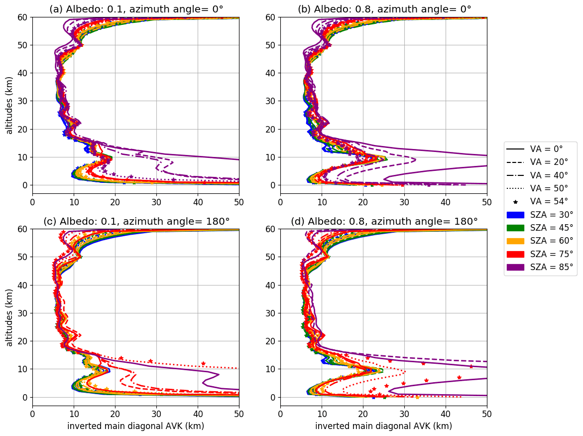
Figure 4Vertical resolution of the retrieval for all simulations with the Chinese polluted ozone profile. The panels show the different combinations of the surface albedo (0.1 and 0.8) and relative azimuth angles (0 and 180∘). Each panel displays the results for 25 combinations of VA and SZA.
A measure for independent pieces of information in the retrieved ozone profiles is provided by the number of degrees of freedom (DOF) determined from the trace of the averaging kernel matrix (). About 6.5 independent variables (from 6.3 for the south polar scenario to 6.7 for the polluted China case) can be retrieved in the altitude range between 0 and 60 km. This corresponds to a mean vertical resolution of about 9 km. Between 0 and 18 km, the synthetic retrievals show around 1.5 DOF. This means that somewhat more information than the total ozone content can be determined in the troposphere. In summary, profile information in the troposphere is severely limited and thus dependent on the a priori ozone profile.
It should be noted here that the number of independent variables might change in the retrievals using real TROPOMI data because of additional pseudo-absorbers which cannot be applied to the synthetic data. These pseudo-absorbers serve to compensate for inestimable calibration errors in the measured radiation.
The UV channels of TROPOMI have been the subject of intensive analysis and calibration before launch and during space operation (Ludewig et al., 2020). First tests with our retrieval applied to the most recent V2 TROPOMI spectral data revealed, however, large deviations in the retrieved ozone profiles, especially in the altitude range above 40 km. Therefore we decided to introduce additional spectral corrections as part of the retrieval. This type of correction, often referred to as vicarious calibration or soft calibration, is described, for example, in Liu et al. (2010). The approach is to simulate TROPOMI radiance for a selected set of measurements using ozone profiles from a comparison instrument, here MLS/Aura, and use the difference of the simulated to the TROPOMI-measured radiance as the calibration correction. To this end, four orbits were selected at intervals of 3 months: orbit 3704 (1 July 2018), 5005 (1 October 2018), 6225 (26 December 2018), and 7642 (5 April 2019). The orbits were required to be cloud-free over the largest area possible. The spread of orbit dates allows us to check the stability of the calibration correction with time. Forward simulations were performed with the SCIATRAN model for all cloud-free pixels (cloud content <10 %). In contrast to the retrieval runs, the RTM calculations were performed with rotational Raman scattering and polarisation to make them as similar as possible to the measurements. The ozone profiles from the nearest MLS measurements were used to initialise SCIATRAN. Below the tropopause, the profiles were supplemented by MERRA-2 reanalyses (Gelaro et al., 2017) as already provided in the MLS data files. Allowing a maximum 1000 km between MLS and TROPOMI pixels, we assume not to introduce a significant systematic error in the tropics, as ozone distribution is relatively homogeneous in this region. At higher latitudes, atmospheric dynamics may lead to higher variability. Here, TROPOMI measurements were only simulated if total ozone from MLS/MERRA-2 and TROPOMI (WFDOAS total ozone) agrees to within 5 %. The surface albedo (retrieved at 378 nm) was taken from the TROPOMI WFDOAS L2 product.
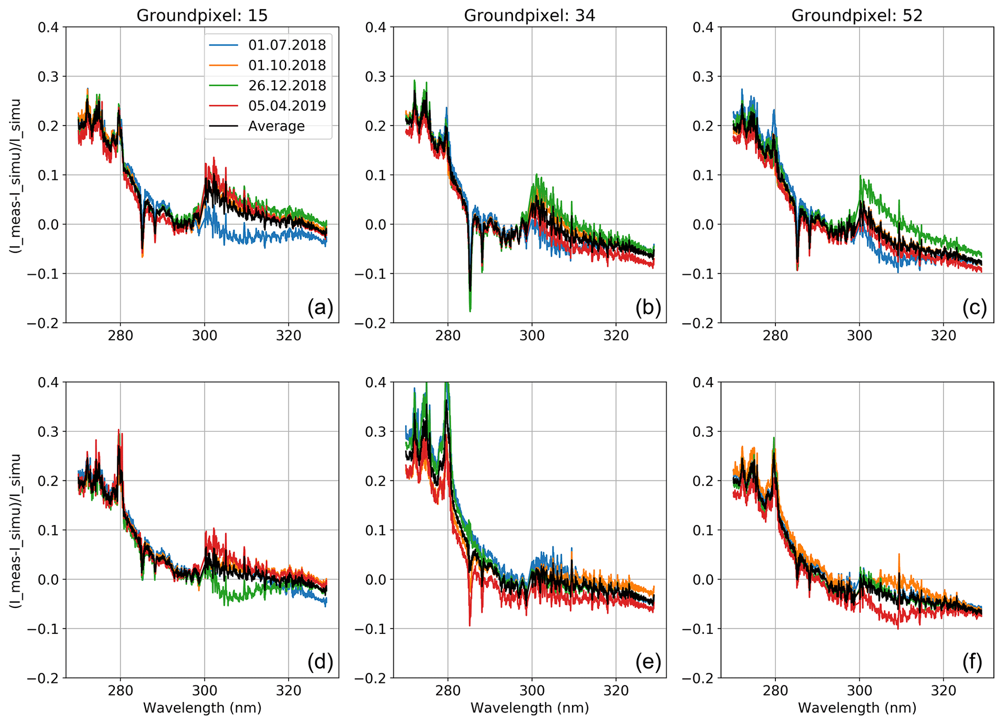
Figure 5Relative differences between the measured and simulated radiances for three detector pixels (viewing angles). (a, b, c) Cloud-free tropical pixels (−20 to 20∘ latitude). (d, e, f) Cloud-free extratropical pixels (−50 to −30∘ and 30 to 50∘ latitude). Black curves represent mean values of four orbits.
The relative difference between the measured and simulated radiances is shown in Fig. 5 exemplarily for ground pixels (viewing angles) 15, 34, and 52 (across-track ground pixel numbers of UV2). Since we identified a slight but stable latitude dependence in all radiance differences, we decided to use independent calibration corrections for the tropics and extra-tropics. In Fig. 5, the upper panels show the differences between the measured and simulated radiances for the tropical pixels (−20 to −20∘ latitude), while the lower panels illustrate the results for the extra-tropical pixels (30 to 50∘ latitude in both hemispheres). The results from the four orbits are displayed in different colours. Overall, the relative difference in UV1 is significantly larger than in UV2. However, the absolute intensities in UV1 are smaller by orders of magnitude. In the spectral range 270–280 nm the relative difference is about +18 % to +25 %, reaching +40 % in the middle of the swath (ground pixel 34) in the extra-tropics (panel e). Such very large values correlate with the variable magnesium absorption lines, which is not accounted for in the retrieval. The overall large differences in the UV1 range are a result of the top of atmosphere limited to 60 km in the RTM that leads to an underestimation of the Rayleigh scattering contribution from layers above 60 km in the RTM and retrieval. The differences between RTM calculations up to 60 and 80 km are shown in Fig. S5. The recalibration spectrum obtained from RTM calculation using layers limited to 60 km can now be interpreted as a combined calibration and Rayleigh scattering correction. Figure S6 shows that this approach is very reasonable and has a positive effect on the retrieved ozone profiles. The variation of the differences between the individual orbits is very small in UV1. In UV2, there are larger differences between individual orbits, as the sensitivity to albedo increases here. The variations between the orbits are the largest in the lower part of UV2 (shorter wavelength). This is because the sensitivity of the radiance to ozone decreases with the wavelength while that to the albedo increases. As a result the maximum of the combined sensitivity is reached around 310 nm. Furthermore the surface albedo retrieved at 378 nm, used as input, may differ from the true albedo at shorter wavelengths. The difference is positive for all orbits at 300 nm (0 % to +10 %) and tends to be negative (0 % to −8 %) towards 330 nm. A closer look into the UV1 band shows a slight decrease of the differences with time in all panels except for ground pixel 52 in the extra-tropics (panel f). To account for this issue we calculate the calibration correction for each ground pixel and for the tropics and extra-tropics independently as the mean relative difference spectra from all four orbits (black curves). The appropriate calibration correction is then used as a pseudo-absorber (one of the three pseudo-absorber mentioned in the previous section) in the preprocessing fit procedure; i.e. a scaling of the calibration correction is allowed. The correction spectra derived from the tropical pixels (−20 to −20∘ latitude) are taken for latitudes up to 30∘, while the spectra derived from the extra-tropics (30 to 50∘ latitude) are applied to all pixels above 30∘ latitude in both hemispheres. Between 20 and 30∘ latitudes the correction spectra are interpolated.
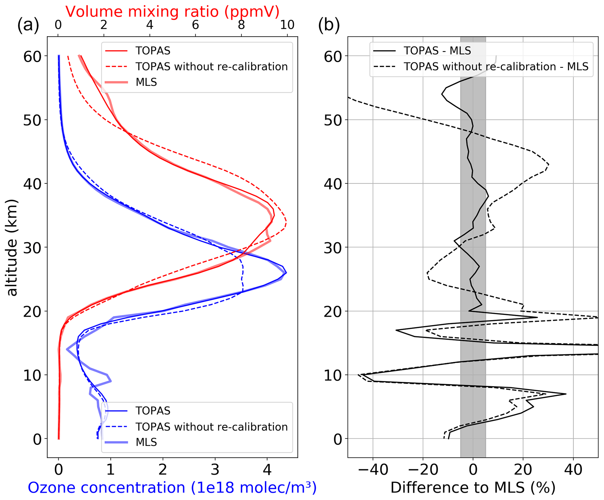
Figure 6Comparison of ozone profiles from the TOPAS retrieval with MLS data for a single TROPOMI pixel (6 April 2019, orbit no. 7664, 16.15∘ latitude, −23.53∘ longitude, SZA: 20.15∘, VA: 11.47∘, and RAZ 6.60∘). Results for the TOPAS retrievals with and without calibration correction are shown. (a) Ozone concentration (blue) and volume mixing ratio (red) from TOPAS/TROPOMI and the collocated MLS measurement. (b) Relative differences between TOPAS retrieval and MLS. The relative differences are identical for both ozone concentration (blue) and volume mixing ratio (red). The grey area marks the ±5 % difference.
Figure 6 demonstrates the effect of the calibration correction in the TOPAS retrieval. For a single TROPOMI pixel the TOPAS retrieval was carried out with and without our calibration correction. In this case a collocated MLS profile was available within 22 min and 28 km of the TROPOMI observation. Figure 6b illustrates the large difference between the ozone profile from the TOPAS algorithm without the calibration correction and the MLS results. The difference increases at high altitudes, which are more sensitive to short wavelengths (<300 nm). The ozone profile from TOPAS including calibration correction agrees very well with MLS between 20 and 50 km. The relative differences are within ±5 %.
To assess the accuracy and quality of the TOPAS algorithm, the retrieved ozone profiles were compared with ozonesondes and ozone lidar data. Both reference data sets have very good quality and a higher vertical resolution than ozone profiles from nadir satellite measurements (see Sect. 2). Ozonesondes are mainly used for comparisons in the troposphere and the lower stratosphere up to a maximum of 35 km. The middle stratosphere (15–50 km) is validated with lidar measurements.
6.1 Ozonesondes
Figure 7 shows the results of the comparison of TROPOMI ozone profiles with ozonesonde measurements. Here, the relative mean difference Δ and its standard deviation SD(Δ) are shown, which are defined by
where ri and si are the data from the ith collocated pair of TROPOMI and sonde measurements, respectively. The relative mean deviation between the TOPAS retrieval results and high-resolution ozonesonde data from all collocations (panel a, black curves) is about 5 % down to about 13 km increasing to about 10 % below. The standard deviation varies between 10 % and 20 % in the lower stratosphere (18–30 km) and between 25 % and 50 % below 18 km. The comparison of the retrieved O3 profiles from TROPOMI and ozonesondes convolved with the TOPAS averaging kernels (panel a, red curves; see Eq. 9) shows that the relative difference is below ±5 % for all altitudes. The difference between the black and red curves is particularly large in the altitude range, where the retrieval is less sensitive (8–18 km).
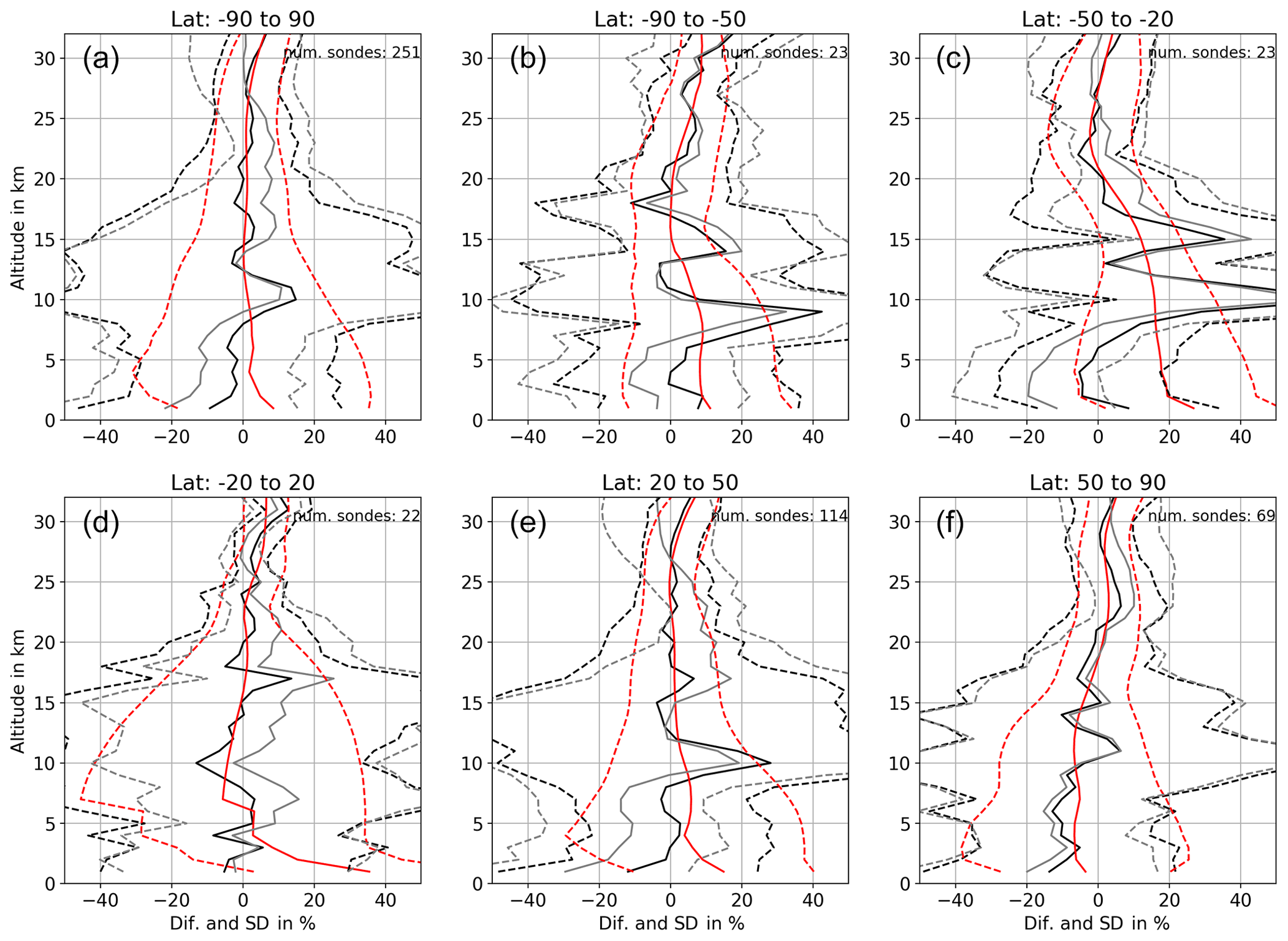
Figure 7Comparison of the ozone profiles retrieved from TROPOMI and those from ozonesondes for different zonal bands. The relative mean difference between the retrieval results and the high-resolution sonde data (solid line), as well as the standard deviation of the differences (dashed line), is shown in black. The comparison with the sonde profiles convolved with the TOPAS averaging kernels is shown in red. In grey the relative difference between the a priori ozone profiles and high-resolution ozonesonde profiles is displayed, along with the corresponding standard deviations.
The results for the northern latitudes and tropics (panels d to f), where the number of available sonde measurements are the highest, look very similar to one another. Above 18 km and below 8 km the relative mean differences are below about ±10 % with 15 % standard deviation. At high and middle southern latitudes (panels b and c), the results are somewhat poorer in the troposphere and lower stratosphere. Between 8 and 18 km differences of +40 % and above can occur.
Also noticeable are the larger differences between the a priori and sonde profiles. As shown in Fig. 2, the results in the altitude range between 8 and 18 km are strongly dependent on the a priori ozone profile. A better choice of the a priori in southern latitudes could possibly improve the retrieval results. With increasing latitudes the viewing geometries change, and especially the SZA becomes larger. There is a connection between SZA and vertical resolution so that at larger angles the vertical resolution between 8 and 18 km strongly decreases. As a consequence, the retrieval remains close to the a priori.
In the lower troposphere (around 5 km) an agreement with the raw ozonesonde profiles within 10 % is observed in all latitude bands, which coincides with the increased vertical resolution found in the altitude range around 5 km; see Fig. 4. As the difference of the a priori to the sonde profiles (grey) is generally larger than that for the retrieved profiles, we can say that the retrieval improves the ozone knowledge in this altitude range for all latitude bands. But we have to note that the standard deviation, in comparison to the a priori, remains almost the same.
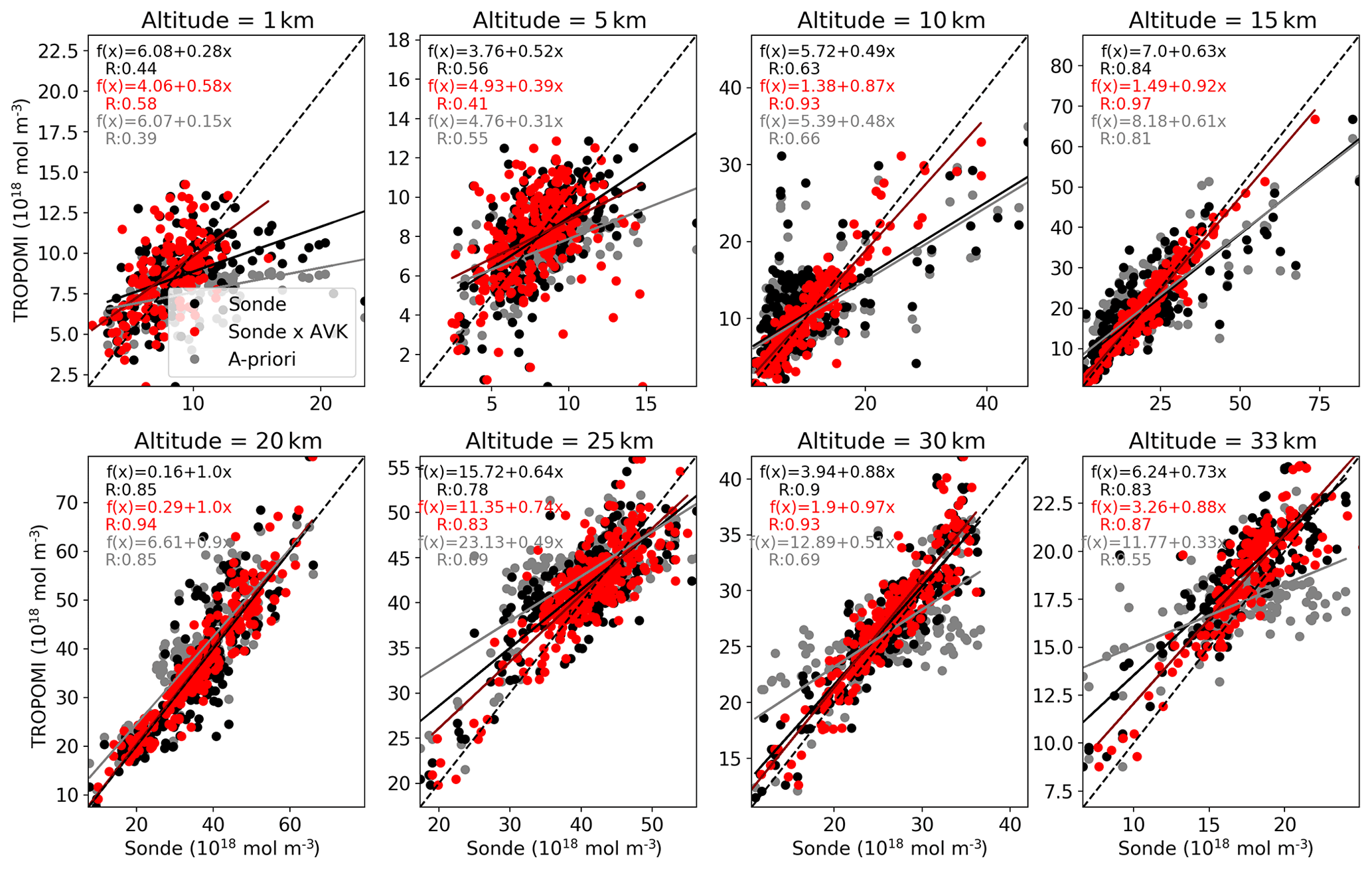
Figure 8Scatter plot of collocated TROPOMI and ozonesonde profiles, the latter with and without convolving with TOPAS averaging kernels (red and black, respectively) for different altitudes (note different scales). The comparison between a priori and sonde profiles is shown in grey. The solid lines show the linear fit. The R value is indicated in the top left corner of each panel (also black and red). The ideal 1:1 curve is plotted as a dashed line.
Figure 8 illustrates the quality of the retrieval at different altitudes in a scatter plot. Again, the retrieval is compared with ozonesondes with (red) and without the convolution with the TOPAS averaging kernels (black). The linear regression is plotted as a solid line (red and black), and the dashed line marks the ideal 1:1 curve. At 1 and 5 km altitude the scatter is wide, and also the R value is small. At 10 km the convolution of the sonde profiles with TOPAS AKs improves the comparison because here the information content is the lowest. The best agreement is found at altitudes 15, 20, and 30 km. The R value here is above 0.8 (0.9 after convolving with AKs), and the linear regression is close to the 1:1 line. At 25 and 33 km the scatter is a little bit larger, but with R values larger than 0.7 the agreement is still good. The slope of the linear regression lines (black and red) improves for each altitude shown in comparison to the a priori slope (grey). In regions where the information content is very limited (10 and 15 km), only the comparison to ozonesondes with applied AKs shows improvement.
6.2 Lidar
Figure 9 shows the relative mean differences (solid line) and the standard deviations (dashed line) between the retrieved profiles form TROPOMI and lidar data (black) for five individual stations and the all-station average (panel a). In addition, the difference between the TOPAS results and the collocated MLS ozone profiles (convolved with TOPAS averaging kernels) is shown in green. When all stations are considered, the deviations between 15 and 45 km are below ±5 % (grey bar). There is a small positive bias between 25 and 45 km that comes mainly from the Table Mountain station data set, which contains the largest number of comparison profiles. The standard deviation of the differences is about 10 % in the range of 20 to 40 km. The comparison with lidar profiles convolved with TOPAS averaging kernels (red) shows nearly the same results for the mean relative difference but a smaller standard deviation above 40 km and below 20 km. A closer look at the individual station reveals generally good agreement but also individual station-dependent deviations. For OHP, Hohenpeißenberg, and Lauder, no larger differences are identified. At Table Mountain there is a stronger negative peak of −9 % around 20 km. Above this altitude a positive bias of up to +10 % increasing with height is observed. The comparison to MLS also shows the negative peak at 20 km but does not show the positive bias at higher altitudes. At Mauna Loa there is a positive bias of +10 % between 25 and 30 km that is also present in the comparison with MLS.

Figure 9Comparison between TROPOMI ozone profile retrieval and the results from five different lidar stations and all-station average. The colours are the same as in Fig. 7 but for lidar instead of ozonesonde data. In addition, the difference between the TROPOMI ozone profile retrieval and MLS results convolved with the TOPAS averaging kernels is shown in green. Only collocated MLS profiles are used (distance <1000 km and time <2 h).
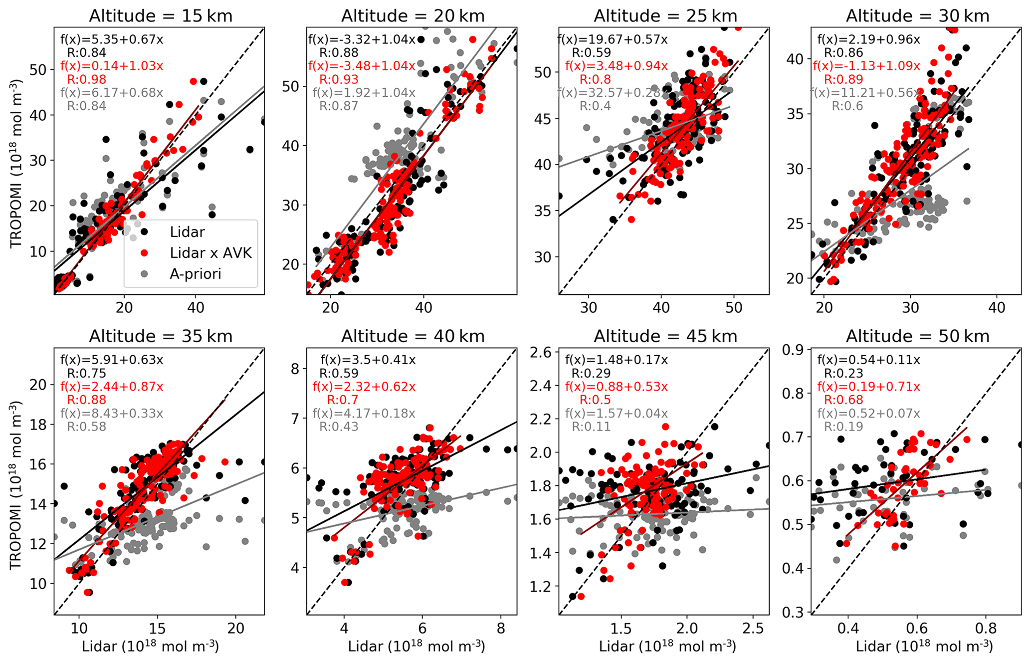
Scatter plots at individual altitude layers are presented in Fig. 10. The colours and lines are assigned in exactly the same way as for the ozonesonde validation shown in Fig. 8. From the scatter plots (Fig. 10), it is evident that in the altitude range between 15 and 40 km the agreement is very good, with R values above 0.6 both with and without convolving with TOPAS averaging kernels. An exception is the altitude of 25 km, where the spread gets larger and the R value lower. At altitudes above 45 km the sensitivity of the TOPAS retrieval decreases, and the agreement after convolving the lidar data with TOPAS averaging kernels is much better. It is notable that above 40 km the TOPAS retrieval shows smaller variability than lidar data. It is not yet known if this is a consequence of the lower sensitivity of the TOPAS retrieval or the lower precision of lidar measurements. Similar to the ozonesonde results, the slope of the linear regression is improving in comparison to the a priori.
As a first application, we show in Fig. 11 an example of a global distribution of TROPOMI ozone for 1 October 2018. Here, the vertical structure of ozone is represented by the subcolumns within the following atmospheric layers: 0–8, 8–18, and 18–25 km, as well as five layers with 5 km thickness between 25 and 50 km. The thickness of each layer roughly represents the vertical resolution of the retrieval in this altitude region in accordance with the results of the sensitivity study and validation. In the 0–8 km subcolumn (a), large variations of ozone are observed, which are believed to be the reason for higher standard deviations seen in the ozonesonde validation. This also reflects the high natural variability in the troposphere due to dynamic processes and local pollution sources. In general the tropical wave one pattern (Sauvage et al., 2006) is well reproduced (low ozone in the Pacific, higher ozone in the South Atlantic). Furthermore, it is noticeable that areas with low ozone levels are related to regions with high cloud coverage.
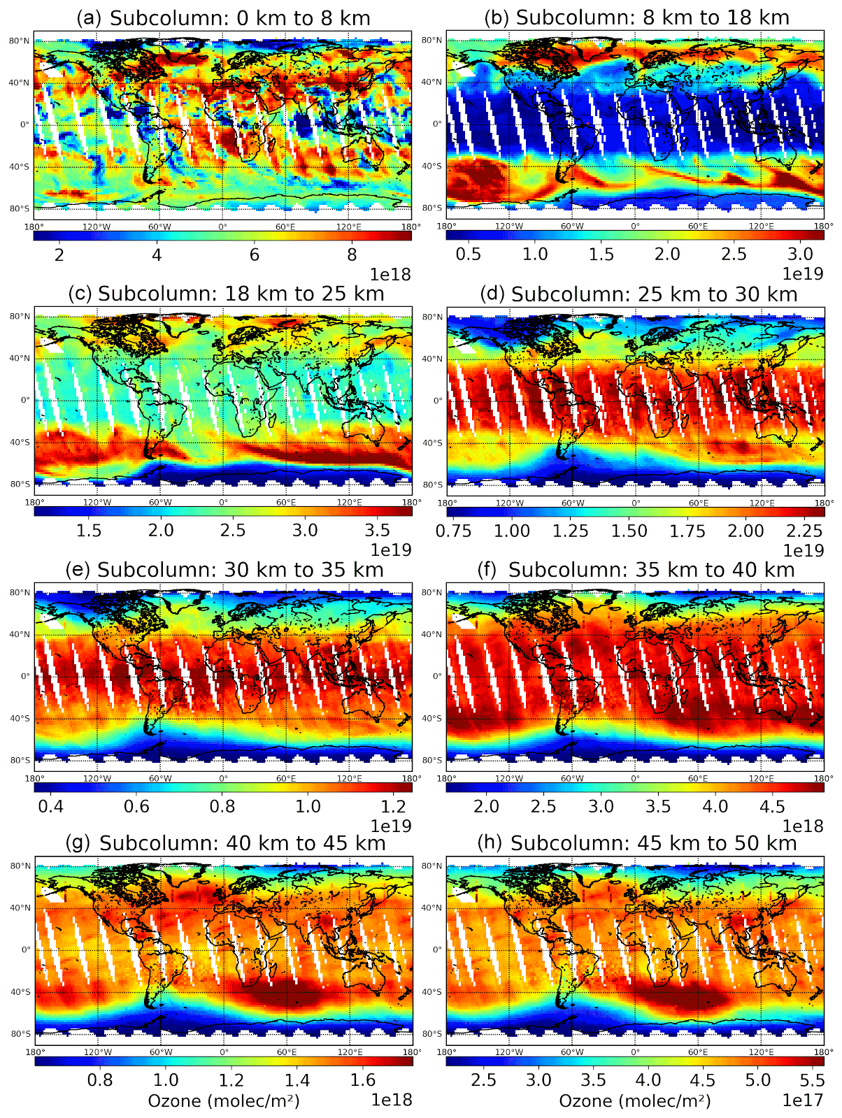
Figure 11TROPOMI ozone subcolumns for selected atmospheric layers for 1 October 2018. Each subcolumn has its own colour scale. The vertical thicknesses of the layers roughly approximate the vertical resolution of the ozone profiles.
In the 8–18 km layer, strong latitude gradients and rather large variabilities are observed. Most noticeable are large areas with high ozone density at middle and high latitudes, which can be identified as ozone streamers in the lower stratosphere and are related to dynamics in the atmosphere. In this altitude layer, the TOPAS retrieval has its lowest sensitivity in general, but a distinction must be made between the lower and higher latitudes (see Fig. 12d). While there is nearly no information of vertical structure in the tropics, the ozone retrieval results in the higher latitudes are reliable. Between 18 and 25 km, the peak of the ozone number density profile is located, and the range of ozone concentration variations is the largest. The largest ozone densities occur in the southern mid-latitudes, while the lowest concentrations are seen in the polar vortex. This is a typical situation in the Southern Hemisphere spring time. The ozone hole seen at polar latitudes is close to its largest extent at this time of the year. We note that the complete coverage of Antarctica is not possible as TROPOMI does not measure during polar night. From the 25–30 km layer upward, the latitude gradient of the ozone number density is reversed, with maximum values occurring now in the tropics. At higher latitudes of both hemispheres, rather low ozone values are observed. The layers 30–35 and 35–40 km show similar ozone distributions to the layer below but appear much smoother. That is to be expected because the retrieval sensitivity reaches its maximum at these altitudes. Also, according to the validation results, no significant systematic errors are to be expected in these layers. The uppermost columns at 40–45 and 45–50 km show the lowest overall ozone levels with a few small-scale variations but a pronounced ozone maximum above the southern Indian Ocean, which extends into the South Atlantic Ocean.
From 25 km upward, the South Atlantic Anomaly (SAA) impact can be observed that results in larger scattering in the retrieved ozone values. The lower wavelength range (below 300 nm) is more strongly affected by the SAA, which leads to the largest uncertainties in high-altitude ozone. If necessary, the SAA region can be filtered out easily by the given flags in the TROPOMI L1B data product.
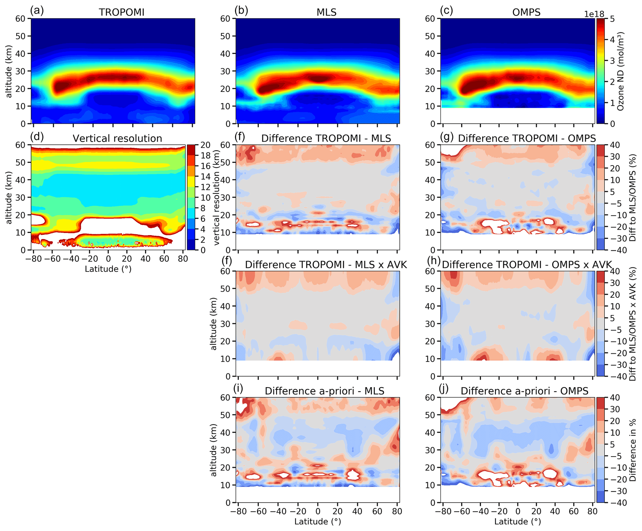
Figure 12(a–c) The zonal mean ozone number density vertical distribution from TROPOMI (a), MLS (b), and OMPS (c) for 1 October 2018. (d) The mean vertical resolution of the TROPOMI retrieval. (e) The relative mean difference between TROPOMI and MLS results. (f) The relative mean difference between TROPOMI and OMPS results. (g, h) Same as (e) and (f) but for MLS and OMPS data convolved with TOPAS averaging kernels. (i, j) Relative mean difference between the TOPAS a priori ozone profiles (climatology) and MLS (i) or OMPS (j) measurements.
Figure 12a shows the zonal mean ozone number density as a function of the altitude and latitude for 1 October 2018. All 14 orbits were binned at 1∘ latitude and averaged. The ozone maxima at about 25 km in the tropics and at about 20 km at southern mid-latitudes are clearly seen. Furthermore, a slight curvature of the ozone peak region with decreasing the peak altitude towards the poles is evident. In the high southern latitudes, the Arctic spring ozone hole is notable. The mean vertical resolution, shown in Fig. 12d, is determined from the inverse main diagonal elements of the TOPAS averaging kernel matrix. Between 20 and 45 km, the vertical resolution ranges from 6 to 10 km. Below 20 km, it strongly depends on the latitude. Between −50 and 50∘, the vertical resolution between 10 and 20 km is coarser than 20 km, indicating that there is almost no vertical information from these altitudes. Below 10 km it improves to 6–8 km between −30 and 50∘, indicating that one piece of independent information can be retrieved. The sensitivity study (Sect. 4.2) showed that the ozone profile retrieval below 18 km strongly depends on the used a priori profile. Thus, in this altitude region, retrieved ozone profiles must always be considered with special caution. The middle and right panels of Fig. 12 show the zonal mean ozone number densities from the MLS and OMPS measurements, respectively, as well as their differences to the TROPOMI results. The closest MLS and OMPS profiles were selected for each retrieved TROPOMI pixel (maximum 1.5 h time difference and 1000 km distance). The direct comparison with MLS, i.e. without convolving MLS data with TOPAS averaging kernels (panel e), shows a good agreement between 20 and 50 km, with differences being mostly below ±10 %. Between 20 and 30 km, there are several spots, with the differences reaching ±20 %. Above 50 km, where the TOPAS retrieval has a low sensitivity, positive differences of up to +20 % in the mid-latitudes and tropics are observed. At high southern latitudes, the positive differences increase to about 40 %, while for high northern latitudes, negative differences are seen. Below 20 km, small-scale patterns with higher differences are evident. Below 15 km, the comparison results are less reliable as the precision of MLS data significantly decreases (Livesey et al., 2020). The comparison with OMPS data (panel f) shows very similar patterns as for MLS. Overall the negative differences are somewhat more prominent. If MLS and OMPS ozone profiles are convolved with TOPAS averaging kernels to account for differences in the vertical resolution, the agreement significantly improves. For MLS data (panel g), differences above ±10 % only occur at high solar zenith angles (highest latitudes). Between 20 and 50 km, agreement below ±5 % is reached almost everywhere, except for a narrow range around 30 km in the tropics and at high northern latitudes, where positive deviations of up to +10 % occur. Above 50 km, positive differences of up to +20 % occur, while below 20 km, mainly negative differences of up to −20 % are observed. Again the comparison with OMPS data (panel h) is very similar to that with MLS, but the differences are somewhat larger. In the bottom panels, the comparison between TOPAS a priori ozone profiles and retrieval results from MLS (panel i) and OMPS (panel j) is shown. From this, it can be seen that the TOPAS retrieval improves the ozone profiles in all regions.
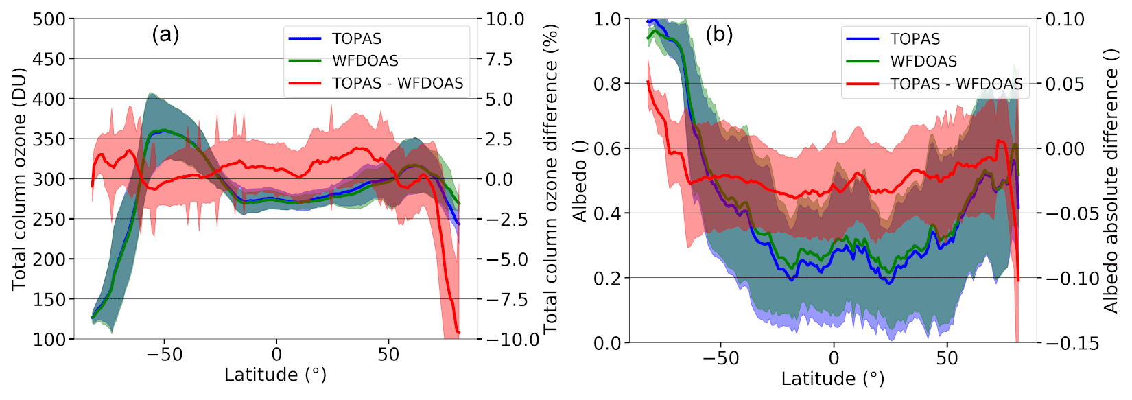
Figure 13Comparison of the TROPOMI total ozone (a) and albedo (b) resulting from the TOPAS ozone profile retrieval and the WFDOAS total ozone product. The data were averaged over all orbits from 1 October 2018. The retrieval results are displayed in blue (TOPAS total ozone) and green (TROPOMI WFDOAS total ozone). Shaded areas mark the standard deviations of the means. The mean difference and the associated standard deviation are plotted in red. Both albedo and total column from TROPOMI WFDOAS are used as a priori assumptions in the TOPAS ozone profile retrieval.
Finally, the retrieved albedo and the total ozone calculated from the retrieved vertical profiles are discussed. The total ozone column and albedo determined from TROPOMI WFDOAS are used to initialise the TROPOMI profile retrieval. The total ozone column information is used to select the proper a priori climatological ozone profile. Figure 13 compares the retrieved albedo and the zonal mean total ozone from all retrieved profiles with the values from the TROPOMI WFDOAS retrieval as a function of latitude. The total ozone (panel a) agrees very well up to about 70∘ N. Both low total ozone values at high southern latitudes and high values at middle latitudes are well represented. The mean difference is below ±2 %, with a standard deviation of about 2 %. Only at high northern latitudes are larger differences of up to −9 % evident. As discussed above, at large solar zenith angles, ozone in the lower atmosphere becomes less visible and is thus not well retrieved. This then results in the contribution from the a priori profile being larger in the total ozone column. The albedo (panel b) shows a stronger variation due to its natural characteristics. Again, very high values at high southern latitudes (due to ice) and low values in the tropics are well captured by both data sets. The mean difference shows a slightly negative bias of up to −0.025, with a standard deviation of about 0.025. However, it should be noted that the albedos in the different retrievals are not derived from the same wavelength ranges. Furthermore, disturbances in the ozone profile retrieval can influence or be compensated by changes in the albedo, since both are derived from the same wavelength range. Above 70∘ N (and high solar zenith angles), the albedo difference increases significantly up to −0.1.
We developed a new TOPAS algorithm based on the first-order Tikhonov regularisation to retrieve the vertical distributions of ozone from TROPOMI measurements in the wavelength range from 270 to 329 nm. In the sensitivity study, we estimated the retrieval quality using synthetic spectra adapted to TROPOMI. We found that the quality of the ozone profile retrieval depends on the viewing geometry, albedo, and the a priori ozone profile. In optimum cases (small solar zenith angles and large albedo), deviations of the individually retrieved profiles from the truth are within ±5 % in the stratosphere. In the troposphere, the agreement is strongly dependent on the a priori profile. Compared to the a priori ozone profile, the retrieval improves the result but can barely compensate differences of more than ±25 % between the a priori and true profiles. If the true profile is convolved with the averaging kernels, differences are generally within ±10 % in the entire altitude range considered (0–60 km). For all simulated scenarios, the vertical resolution of the retrieval is 6–9 km in the stratosphere (18–50 km), getting worse in the lowermost stratosphere and the troposphere (up to 15 km). In the troposphere, the vertical resolution degrades with increasing solar zenith angle. Above 75∘ SZA, almost no information from the troposphere is available. The number of independent variables (degrees of freedom) which can be retrieved over the entire altitude range is around 6, which corresponds to a mean vertical resolution of 10 km from 0 to 60 km altitude.
In addition to improvements in the UV radiometric calibration in version 2 of TROPOMI level 1 data (Ludewig et al., 2020), a radiometric calibration correction was determined using radiative transfer simulations and MLS ozone profiles. For the shortest wavelengths, radiometric adjustments of +20 % and more are needed. The correction drops below ±10 % for longer wavelengths.
The TOPAS ozone profile retrieval was validated by comparisons with ozonesonde and stratospheric ozone lidar data. For the limited TROPOMI data set available so far, we found very good agreement with both validation data sets. The validation with ozonesondes shows good agreement in the lower stratosphere, with deviations of less than ±10 % at all latitudes in the altitude range 18–30 km. The standard deviation of the mean differences is about 10 %. Below 18 km, the mean difference and the standard deviation increases strongly but decreases when the sondes are convolved with the TOPAS averaging kernels.
The validation with lidar measurements shows a bias within ±5 % between 15–45 km. The standard deviation is about 10 %. The convolution of the lidar profiles with TOPAS averaging kernels barely changes the result because of a high sensitivity and relatively good vertical resolution in the stratosphere.
By applying the TOPAS retrieval to a full day of TROPOMI measurements (14 orbits), we demonstrated the high potential of the ozone profile retrieval, enabling us to determine highly spatially resolved vertical profiles. Important dynamical features in the atmosphere such as streamers and seasonal events such as the ozone hole can be detected. A comparison with ozone profiles from MLS and OMPS limb measurements shows typically good agreement to within ±5 % between 20 and 50 km. If the averaging kernels are taken into account, the differences above 50 km and below 20 km also get smaller, reaching about ±20 %. Good agreement in total ozone compared to TROPOMI WFDOAS (within ±2 %) was found.
When a continuous L1B version 2 data set is made available for TROPOMI, we plan to close the data gaps by processing these data. This will enable us to extend the validation using a larger data set from early 2018 until present and to investigate time series. The verification of the temporal stability of the ozone profile retrieval is still ongoing. The assessment of the calibration correction using MLS data as implemented in this study is also of particular importance in this context. If the finding of this study, that a temporally independent but spectrally dependent radiometric correction factor is sufficient and holds for the full data set, the final data product can be created which is independent of MLS apart of the initial correction. That would enable the use of TROPOMI ozone profiles for trend analysis and monitoring. Thus, the goal to use TROPOMI measurements to mitigate consequences of a possible lack of limb instruments may become feasible.
All data and source codes are available upon request from Nora Mettig (mettig@iup.physik.uni-bremen.de) or Mark Weber (weber@uni-bremen.de). The L1B version of the S5P data is available upon request to the S5P Validation Team. MLS ozone profiles can be downloaded from the NASA Goddard Space Flight Center Earth Sciences Data and Information Services Center (GES DISC; Schwartz et al., 2020, https://doi.org/10.5067/Aura/MLS/DATA2516). OMPS limb ozone profiles are available upon request from Carlo Arosio (carloarosio@iup.physik.uni-bremen.de), and S5P WFDOAS total ozone and albedo data are available from Mark Weber. Ozonesonde data from the WOUDC can be downloaded from https://doi.org/10.14287/10000008 (WOUDC Ozonesonde Monitoring Community et al., 2021). Ozonesonde data from SHADOZ (Witte et al., 2017, https://doi.org/10.1002/2016JD026403; Thompson et al., 2017, https://doi.org/10.1002/2017JD027406; Witte et al., 2018, https://doi.org/10.1002/2017JD027791; Sterling et al., 2018, https://doi.org/10.5194/amt-11-3661-2018). The stratospheric lidar data used in this publication were obtained from Richard Querel, Thierry Leblanc, Sophie Godin Beekmann, and Wolfgang Steinbrecht as part of the Network for the Detection of Atmospheric Composition Change (NDACC) and are available through the NDACC website http://www.ndaccdemo.org/ (last access: 9 September 2021, Network for Detection of Atmospheric Composition Change, 2021).
The supplement related to this article is available online at: https://doi.org/10.5194/amt-14-6057-2021-supplement.
NM developed the ozone profile retrieval algorithm and performed sensitivity tests and validation. MW and AR provided direct advice and support. AR made the SCIATRAN model code available. NM, MW, AR, and JPB defined the paper structure and content. CA provided the OMPS ozone profile data and MW the S5P WFDOAS total ozone and albedo data. PV provided support by discussing the TROPOMI measurements, the recalibration, and the ozone profile retrieval. AT, RQ, TL, SGB, RK, and MT provided ozonesonde and lidar data for the validation. All authors reviewed the paper.
The authors declare that they have no conflict of interest.
Publisher’s note: Copernicus Publications remains neutral with regard to jurisdictional claims in published maps and institutional affiliations.
The S5P L1b version 2 data have been provided by ESA/KNMI via the S5P validation team (S5P-VT) activities. We acknowledge all ozonesonde providers and their funding agencies for performing regular sonde measurements and thank the WOUDC and SHADOZ network for archiving these data. The same applies to the teams from all the lidar stations we used. Ozone profiles of the MLS limb measurements have been provided by NASA.
This study has been supported and funded by the BMWi/DLR project “S5P Datennutzung” (grant no. 50EE1811A), the University of Bremen, and the federal state Bremen. All calculations reported here were performed on the HPC facilities of the IUP, University of Bremen, funded under DFG/FUGG
(grant nos. INST 144/379-1 and INST 144/493-1). Part of this research work was carried out at the Jet Propulsion Laboratory, California Institute of
Technology, under a contract with the National Aeronautics and Space
Administration (grant no. 80NM0018D004).
The article processing charges for this open-access publication were covered by the University of Bremen.
This paper was edited by Diego Loyola and reviewed by three anonymous referees.
Arosio, C., Rozanov, A., Malinina, E., Eichmann, K.-U., von Clarmann, T., and Burrows, J. P.: Retrieval of ozone profiles from OMPS limb scattering observations, Atmos. Meas. Tech., 11, 2135–2149, https://doi.org/10.5194/amt-11-2135-2018, 2018. a
Bates, D. R. and Nicolet, M.: The photochemistry of atmospheric water vapor, J. Geophys. Res., 55, 301–327, https://doi.org/10.1029/JZ055i003p00301, 1950. a
Bhartia, P. K., McPeters, R. D., Mateer, C. L., Flynn, L. E., and Wellemeyer, C.: Algorithm for the estimation of vertical ozone profiles from the backscattered ultraviolet technique, J. Geophys. Res., 101, 18793–18806, https://doi.org/10.1029/96JD01165, 1996. a
Burrows, J. P., Hölzle, E., Goede, A., Visser, H., and Fricke, W.: SCIAMACHY–scanning imaging absorption spectrometer for atmospheric chartography, Acta Astronaut., 35, 445–451, https://doi.org/10.1016/0094-5765(94)00278-T, 1995. a
Burrows, J. P., Weber, M., Buchwitz, M., Rozanov, V., Ladstätter-Weißenmayer, A., Richter, A., DeBeek, R., Hoogen, R., Bramstedt, K., Eichmann, K.-U., Eisinger, M., and Perner, D.: The Global Ozone Monitoring Experiment (GOME): Mission Concept and First Scientific Results, J. Atmos. Sci., 56, 151–175, https://doi.org/10.1175/1520-0469(1999)056<0151:TGOMEG<2.0.CO;2, 1999. a, b
Chance, K. and Kurucz, R. L.: An improved high-resolution solar reference spectrum for earth's atmosphere measurements in the ultraviolet, visible, and near infrared, J. Quant. Spectrosc. Ra., 111, 1289–1295, https://doi.org/10.1016/j.jqsrt.2010.01.036, 2010. a, b
Chapman, S.: A theory of upper-atmospheric ozone, Edward Stanford, London, 1930. a
Cisewski, M., Zawodny, J., Gasbarre, J., Eckman, R., Topiwala, N., Rodriguez-Alvarez, O., Cheek, D., and Hall, S.: The Stratospheric Aerosol and Gas Experiment (SAGE III) on the International Space Station (ISS) Mission, in: Sensors, Systems, and Next-Generation Satellites XVIII, edited by: Meynart, R., Neeck, S. P., and Shimoda, H., SPIE, 924107, https://doi.org/10.1117/12.2073131, 2014. a
Coldewey-Egbers, M., Weber, M., Lamsal, L. N., de Beek, R., Buchwitz, M., and Burrows, J. P.: Total ozone retrieval from GOME UV spectral data using the weighting function DOAS approach, Atmos. Chem. Phys., 5, 1015–1025, https://doi.org/10.5194/acp-5-1015-2005, 2005. a, b
de Beek, R., Weber, M., Rozanov, V., Rozanov, A., Richter, A., and Burrows, J.: Trace gas column retrieval – an error assessment study for GOME-2, Adv. Space Res., 34, 727–733, https://doi.org/10.1016/j.asr.2003.06.042, 2004. a
De Mazière, M., Thompson, A. M., Kurylo, M. J., Wild, J. D., Bernhard, G., Blumenstock, T., Braathen, G. O., Hannigan, J. W., Lambert, J.-C., Leblanc, T., McGee, T. J., Nedoluha, G., Petropavlovskikh, I., Seckmeyer, G., Simon, P. C., Steinbrecht, W., and Strahan, S. E.: The Network for the Detection of Atmospheric Composition Change (NDACC): history, status and perspectives, Atmos. Chem. Phys., 18, 4935–4964, https://doi.org/10.5194/acp-18-4935-2018, 2018. a
Deshler, T., Mercer, J. L., Smit, H. G. J., Stubi, R., Levrat, G., Johnson, B. J., Oltmans, S. J., Kivi, R., Thompson, A. M., Witte, J., Davies, J., Schmidlin, F. J., Brothers, G., and Sasaki, T.: Atmospheric comparison of electrochemical cell ozonesondes from different manufacturers, and with different cathode solution strengths: The Balloon Experiment on Standards for Ozonesondes, J. Geophys. Res., 113, D04307, https://doi.org/10.1029/2007JD008975, 2008. a
ESA/KNMI: Ozone Profiles, Tropomi, available at: http://www.tropomi.eu/data-products/ozone-profiles, last access: 31 May 2021a. a
ESA/KNMI: ISRF Dataset, Tropomi [data set], available at: http://www.tropomi.eu/data-products/isrf-dataset, last access: 31 May 2021b. a
EUMETSAT: Metop satellites – future Missions, available at: https://www.eumetsat.int/our-satellites/metop-series?sjid=future, last access: 26 May 2021. a
Farman, J. C., Gardiner, B. G., and Shanklin, J. D.: Large losses of total ozone in Antarctica reveal seasonal interaction, Nature, 315, 207–210, https://doi.org/10.1038/315207a0, 1985. a
Fletcher, K. and McMullan, K.: Sentinel 5 Precursor: ESA's Atmospheric Chemistry and Pollution-Monitoring Mission, vol. ESA SP-1332, European Space Agency, Leiden, The Netherlands, 2016. a
Flynn, L., Long, C., Wu, X., Evans, R., Beck, C. T., Petropavlovskikh, I., McConville, G., Yu, W., Zhang, Z., Niu, J., Beach, E., Hao, Y., Pan, C., Sen, B., Novicki, M., Zhou, S., and Seftor, C.: Performance of the Ozone Mapping and Profiler Suite (OMPS) products, J. Geophys. Res.-Atmos., 119, 6181–6195, https://doi.org/10.1002/2013JD020467, 2014. a
Froidevaux, L., Jiang, Y. B., Lambert, A., Livesey, N. J., Read, W. G., Waters, J. W., Browell, E. V., Hair, J. W., Avery, M. A., McGee, T. J., Twigg, L. W., Sumnicht, G. K., Jucks, K. W., Margitan, J. J., Sen, B., Stachnik, R. A., Toon, G. C., Bernath, P. F., Boone, C. D., Walker, K. A., Filipiak, M. J., Harwood, R. S., Fuller, R. A., Manney, G. L., Schwartz, M. J., Daffer, W. H., Drouin, B. J., Cofield, R. E., Cuddy, D. T., Jarnot, R. F., Knosp, B. W., Perun, V. S., Snyder, W. V., Stek, P. C., Thurstans, R. P., and Wagner, P. A.: Validation of Aura Microwave Limb Sounder stratospheric ozone measurements, J. Geophys. Res., 113, D15S20, https://doi.org/10.1029/2007JD008771, 2008. a
Gelaro, R., McCarty, W., Suárez, M. J., Todling, R., Molod, A., Takacs, L., Randles, C., Darmenov, A., Bosilovich, M. G., Reichle, R., Wargan, K., Coy, L., Cullather, R., Draper, C., Akella, S., Buchard, V., Conaty, A., da Silva, A., Gu, W., Kim, G.-K., Koster, R., Lucchesi, R., Merkova, D., Nielsen, J. E., Partyka, G., Pawson, S., Putman, W., Rienecker, M., Schubert, S. D., Sienkiewicz, M., and Zhao, B.: The Modern-Era Retrospective Analysis for Research and Applications, Version 2 (MERRA-2), J. Climate,30, 5419–5454, https://doi.org/10.1175/JCLI-D-16-0758.1, 2017. a
Hasekamp, O. P. and Landgraf, J.: Ozone profile retrieval from backscattered ultraviolet radiances: The inverse problem solved by regularization, J. Geophys. Res., 106, 8077–8088, https://doi.org/10.1029/2000JD900692, 2001. a, b
Hassler, B., Petropavlovskikh, I., Staehelin, J., August, T., Bhartia, P. K., Clerbaux, C., Degenstein, D., Mazière, M. D., Dinelli, B. M., Dudhia, A., Dufour, G., Frith, S. M., Froidevaux, L., Godin-Beekmann, S., Granville, J., Harris, N. R. P., Hoppel, K., Hubert, D., Kasai, Y., Kurylo, M. J., Kyrölä, E., Lambert, J.-C., Levelt, P. F., McElroy, C. T., McPeters, R. D., Munro, R., Nakajima, H., Parrish, A., Raspollini, P., Remsberg, E. E., Rosenlof, K. H., Rozanov, A., Sano, T., Sasano, Y., Shiotani, M., Smit, H. G. J., Stiller, G., Tamminen, J., Tarasick, D. W., Urban, J., van der A, R. J., Veefkind, J. P., Vigouroux, C., von Clarmann, T., von Savigny, C., Walker, K. A., Weber, M., Wild, J., and Zawodny, J. M.: Past changes in the vertical distribution of ozone – Part 1: Measurement techniques, uncertainties and availability, Atmos. Meas. Tech., 7, 1395–1427, https://doi.org/10.5194/amt-7-1395-2014, 2014. a
Hersbach, H., Bell, B., Berrisford, P., Hirahara, S., Horányi, A., Muñoz-Sabater, J., Nicolas, J., Peubey, C., Radu, R., Schepers, D., Simmons, A., Soci, C., Abdalla, S., Abellan, X., Balsamo, G., Bechtold, P., Biavati, G., Bidlot, J., Bonavita, M., Chiara, G., Dahlgren, P., Dee, D., Diamantakis, M., Dragani, R., Flemming, J., Forbes, R., Fuentes, M., Geer, A., Haimberger, L., Healy, S., Hogan, R. J., Hólm, E., Janisková, M., Keeley, S., Laloyaux, P., Lopez, P., Lupu, C., Radnoti, G., Rosnay, P., Rozum, I., Vamborg, F., Villaume, S., and Thépaut, J.-N.: The ERA5 global reanalysis, Q. J. Roy. Meteor. Soc., 146, 1999–2049, https://doi.org/10.1002/qj.3803, 2020. a
Hoogen, R., Rozanov, V. V., and Burrows, J. P.: Ozone profiles from GOME satellite data: Algorithm description and first validation, J. Geophys. Res., 104, 8263–8280, https://doi.org/10.1029/1998JD100093, 1999. a, b
Huang, G., Liu, X., Chance, K., Yang, K., Bhartia, P. K., Cai, Z., Allaart, M., Ancellet, G., Calpini, B., Coetzee, G. J. R., Cuevas-Agulló, E., Cupeiro, M., De Backer, H., Dubey, M. K., Fuelberg, H. E., Fujiwara, M., Godin-Beekmann, S., Hall, T. J., Johnson, B., Joseph, E., Kivi, R., Kois, B., Komala, N., König-Langlo, G., Laneve, G., Leblanc, T., Marchand, M., Minschwaner, K. R., Morris, G., Newchurch, M. J., Ogino, S.-Y., Ohkawara, N., Piters, A. J. M., Posny, F., Querel, R., Scheele, R., Schmidlin, F. J., Schnell, R. C., Schrems, O., Selkirk, H., Shiotani, M., Skrivánková, P., Stübi, R., Taha, G., Tarasick, D. W., Thompson, A. M., Thouret, V., Tully, M. B., Van Malderen, R., Vömel, H., von der Gathen, P., Witte, J. C., and Yela, M.: Validation of 10-year SAO OMI Ozone Profile (PROFOZ) product using ozonesonde observations, Atmos. Meas. Tech., 10, 2455–2475, https://doi.org/10.5194/amt-10-2455-2017, 2017. a
Hubert, D., Lambert, J.-C., Verhoelst, T., Granville, J., Keppens, A., Baray, J.-L., Bourassa, A. E., Cortesi, U., Degenstein, D. A., Froidevaux, L., Godin-Beekmann, S., Hoppel, K. W., Johnson, B. J., Kyrölä, E., Leblanc, T., Lichtenberg, G., Marchand, M., McElroy, C. T., Murtagh, D., Nakane, H., Portafaix, T., Querel, R., Russell III, J. M., Salvador, J., Smit, H. G. J., Stebel, K., Steinbrecht, W., Strawbridge, K. B., Stübi, R., Swart, D. P. J., Taha, G., Tarasick, D. W., Thompson, A. M., Urban, J., van Gijsel, J. A. E., Van Malderen, R., von der Gathen, P., Walker, K. A., Wolfram, E., and Zawodny, J. M.: Ground-based assessment of the bias and long-term stability of 14 limb and occultation ozone profile data records, Atmos. Meas. Tech., 9, 2497–2534, https://doi.org/10.5194/amt-9-2497-2016, 2016. a
Hubert, D., Heue, K.-P., Lambert, J.-C., Verhoelst, T., Allaart, M., Compernolle, S., Cullis, P. D., Dehn, A., Félix, C., Johnson, B. J., Keppens, A., Kollonige, D. E., Lerot, C., Loyola, D., Maata, M., Mitro, S., Mohamad, M., Piters, A., Romahn, F., Selkirk, H. B., da Silva, F. R., Stauffer, R. M., Thompson, A. M., Veefkind, J. P., Vömel, H., Witte, J. C., and Zehner, C.: TROPOMI tropospheric ozone column data: Geophysical assessment and comparison to ozonesondes, GOME-2B and OMI, Atmos. Meas. Tech. Discuss. [preprint], https://doi.org/10.5194/amt-2020-123, in review, 2020. a
Jaross, G., Bhartia, P. K., Chen, G., Kowitt, M., Haken, M., Chen, Z., Xu, P., Warner, J., and Kelly, T.: OMPS Limb Profiler instrument performance assessment, J. Geophys. Res.-Atmos., 119, 4399–4412, https://doi.org/10.1002/2013JD020482, 2014. a
Jia, J., Rozanov, A., Ladstätter-Weißenmayer, A., and Burrows, J. P.: Global validation of SCIAMACHY limb ozone data (versions 2.9 and 3.0, IUP Bremen) using ozonesonde measurements, Atmos. Meas. Tech., 8, 3369–3383, https://doi.org/10.5194/amt-8-3369-2015, 2015. a
Jiang, Y. B., Froidevaux, L., Lambert, A., Livesey, N. J., Read, W. G., Waters, J. W., Bojkov, B., Leblanc, T., McDermid, I. S., Godin-Beekmann, S., Filipiak, M. J., Harwood, R. S., Fuller, R. A., Daffer, W. H., Drouin, B. J., Cofield, R. E., Cuddy, D. T., Jarnot, R. F., Knosp, B. W., Perun, V. S., Schwartz, M. J., Snyder, W. V., Stek, P. C., Thurstans, R. P., Wagner, P. A., Allaart, M., Andersen, S. B., Bodeker, G., Calpini, B., Claude, H., Coetzee, G., Davies, J., de Backer, H., Dier, H., Fujiwara, M., Johnson, B., Kelder, H., Leme, N. P., König-Langlo, G., Kyro, E., Laneve, G., Fook, L. S., Merrill, J., Morris, G., Newchurch, M., Oltmans, S., Parrondos, M. C., Posny, F., Schmidlin, F., Skrivankova, P., Stubi, R., Tarasick, D., Thompson, A., Thouret, V., Viatte, P., Vömel, H., von der Gathen, P., Yela, M., and Zablocki, G.: Validation of Aura Microwave Limb Sounder Ozone by ozonesonde and lidar measurements, J. Geophys. Res., 112, D24S34, https://doi.org/10.1029/2007JD008776, 2007. a
Johnson, B. J.: Electrochemical concentration cell (ECC) ozonesonde pump efficiency measurements and tests on the sensitivity to ozone of buffered and unbuffered ECC sensor cathode solutions, J. Geophys. Res., 107, 4393, https://doi.org/10.1029/2001JD000557, 2002. a
Kleipool, Q.: Sentinel-5P TROPOMI L1B Radiance product band 1 (UV detector), NASA Goddard Earth Sciences Data and Information Services Center [data set], https://doi.org/10.5067/SENTINEL5P/S5P_L1B_RA_BD1.1, 2018. a
Kroon, M., de Haan, J. F., Veefkind, J. P., Froidevaux, L., Wang, R., Kivi, R., and Hakkarainen, J. J.: Validation of operational ozone profiles from the Ozone Monitoring Instrument, J. Geophys. Res., 116, D18305, https://doi.org/10.1029/2010JD015100, 2011. a
Lamsal, L. N., Weber, M., Tellmann, S., and Burrows, J. P.: Ozone column classified climatology of ozone and temperature profiles based on ozonesonde and satellite data, J. Geophys. Res., 109, D20304, https://doi.org/10.1029/2004JD004680, 2004. a, b, c
Leblanc, T., Sica, R. J., van Gijsel, J. A. E., Godin-Beekmann, S., Haefele, A., Trickl, T., Payen, G., and Liberti, G.: Proposed standardized definitions for vertical resolution and uncertainty in the NDACC lidar ozone and temperature algorithms – Part 2: Ozone DIAL uncertainty budget, Atmos. Meas. Tech., 9, 4051–4078, https://doi.org/10.5194/amt-9-4051-2016, 2016. a
Levelt, P. and Veefkind, P.: ESA CAMELOT study: Challenges in future operational missions for GMES atmospheric monitoring, sentinel 4 and 5, in: EGU General Assembly Conference Abstracts, EGU General Assembly Conference Abstracts, p. 8911, 2009. a
Liu, X., Chance, K., Sioris, C. E., Spurr, R. J. D., Kurosu, T. P., Martin, R. V., and Newchurch, M. J.: Ozone profile and tropospheric ozone retrievals from the Global Ozone Monitoring Experiment: Algorithm description and validation, J. Geophys. Res., 110, D20307, https://doi.org/10.1029/2005JD006240, 2005. a
Liu, X., Bhartia, P. K., Chance, K., Spurr, R. J. D., and Kurosu, T. P.: Ozone profile retrievals from the Ozone Monitoring Instrument, Atmos. Chem. Phys., 10, 2521–2537, https://doi.org/10.5194/acp-10-2521-2010, 2010. a, b
Livesey, N. J., Filipiak, M. J., Froidevaux, L., Read, W. G., Lambert, A., Santee, M. L., Jiang, J. H., Pumphrey, H. C., Waters, J. W., Cofield, R. E., Cuddy, D. T., Daffer, W. H., Drouin, B. J., Fuller, R. A., Jarnot, R. F., Jiang, Y. B., Knosp, B. W., Li, Q. B., Perun, V. S., Schwartz, M. J., Snyder, W. V., Stek, P. C., Thurstans, R. P., Wagner, P. A., Avery, M., Browell, E. V., Cammas, J.-P., Christensen, L. E., Diskin, G. S., Gao, R.-S., Jost, H.-J., Loewenstein, M., Lopez, J. D., Nedelec, P., Osterman, G. B., Sachse, G. W., and Webster, C. R.: Validation of Aura Microwave Limb Sounder O3 and CO observations in the upper troposphere and lower stratosphere, J. Geophys. Res., 113, D15S02, https://doi.org/10.1029/2007JD008805, 2008. a
Livesey, N. J., Read, W. G., Wagner, P. A., Froidevaux, L., Lambert, A., Manney, G. L., Valle, L., Pumphrey, H. C., Santee, M. L., Schwartz, M. J., Wang, S., Fuller, R. A., Jarnot, R. F., Knosp, B. W., Martinez, E., and Lay, R. R.: Aura Microwave Limb Sounder (MLS): Version 4.2x Level 2 and 3 data quality and description document, JPL D-33509 Rev. E, Jet Propulsion Laboratory, California Institute of Technology, Pasadena, California, available at: https://mls.jpl.nasa.gov/data/v4-2_data_quality_document.pdf (last access: 6 September 2021), 2020. a, b
Llewellyn, E. J., Degenstein, D. A., McDade, I. C., Gattinger, R. L., King, R., Buckingham, R., Richardson, E. H., Murtagh, D. P., Evans, W. F. J., Solheim, B. H., Strong, K., and McConnell, J. C.: Osiris – An Application of Tomography for Absorbed Emissions in Remote Sensing, in: Applications of Photonic Technology 2, edited by: Lampropoulos, G. A. and Lessard, R. A., Springer US, Boston, MA, 627–632, https://doi.org/10.1007/978-1-4757-9250-8_98, 1997. a
Loyola, D. G., Gimeno García, S., Lutz, R., Argyrouli, A., Romahn, F., Spurr, R. J. D., Pedergnana, M., Doicu, A., Molina García, V., and Schüssler, O.: The operational cloud retrieval algorithms from TROPOMI on board Sentinel-5 Precursor, Atmos. Meas. Tech., 11, 409–427, https://doi.org/10.5194/amt-11-409-2018, 2018. a
Ludewig, A., Kleipool, Q., Bartstra, R., Landzaat, R., Leloux, J., Loots, E., Meijering, P., van der Plas, E., Rozemeijer, N., Vonk, F., and Veefkind, P.: In-flight calibration results of the TROPOMI payload on board the Sentinel-5 Precursor satellite, Atmos. Meas. Tech., 13, 3561–3580, https://doi.org/10.5194/amt-13-3561-2020, 2020. a, b, c, d, e
Miles, G. M., Siddans, R., Kerridge, B. J., Latter, B. G., and Richards, N. A. D.: Tropospheric ozone and ozone profiles retrieved from GOME-2 and their validation, Atmos. Meas. Tech., 8, 385–398, https://doi.org/10.5194/amt-8-385-2015, 2015. a
Munro, R., Siddans, R., Reburn, W. J., and Kerridge, B. J.: Direct measurement of tropospheric ozone distributions from space, Nature, 392, 168–171, https://doi.org/10.1038/32392, 1998. a
Nair, P. J., Godin-Beekmann, S., Froidevaux, L., Flynn, L. E., Zawodny, J. M., Russell III, J. M., Pazmiño, A., Ancellet, G., Steinbrecht, W., Claude, H., Leblanc, T., McDermid, S., van Gijsel, J. A. E., Johnson, B., Thomas, A., Hubert, D., Lambert, J.-C., Nakane, H., and Swart, D. P. J.: Relative drifts and stability of satellite and ground-based stratospheric ozone profiles at NDACC lidar stations, Atmos. Meas. Tech., 5, 1301–1318, https://doi.org/10.5194/amt-5-1301-2012, 2012. a
Network for the Detection of Atmospheric Composition Change (NDACC): http://www.ndaccdemo.org/, last access: 9 September 2021. a
Orfanoz-Cheuquelaf, A., Rozanov, A., Weber, M., Arosio, C., Ladstätter-Weißenmayer, A., and Burrows, J. P.: Total ozone column retrieval from OMPS-NM measurements, Atmos. Meas. Tech. Discuss. [preprint], https://doi.org/10.5194/amt-2021-61, in review, 2021. a
Purser, R. J. and Huang, H.-L.: Estimating Effective Data Density in a Satellite Retrieval or an Objective Analysis, J. Appl. Meteorol., 32, 1092–1107, https://doi.org/10.1175/1520-0450(1993)032<1092:EEDDIA>2.0.CO;2, 1993. a
Rodgers, C. D.: Inverse methods for atmospheric sounding: Theory and practice, in: Series on atmospheric oceanic and planetary physics: Volume 2, World Scientific, Singapore, https://doi.org/10.1142/3171, 2002. a, b, c, d, e, f, g
Rozanov, A., Bovensmann, H., Bracher, A., Hrechanyy, S., Rozanov, V., Sinnhuber, M., Stroh, F., and Burrows, J. P.: NO2 and BrO vertical profile retrieval from SCIAMACHY limb measurements: Sensitivity studies, Adv. Space Res., 36, 846–854, https://doi.org/10.1016/j.asr.2005.03.013, 2005. a
Rozanov, A., Eichmann, K.-U., von Savigny, C., Bovensmann, H., Burrows, J. P., von Bargen, A., Doicu, A., Hilgers, S., Godin-Beekmann, S., Leblanc, T., and McDermid, I. S.: Comparison of the inversion algorithms applied to the ozone vertical profile retrieval from SCIAMACHY limb measurements, Atmos. Chem. Phys., 7, 4763–4779, https://doi.org/10.5194/acp-7-4763-2007, 2007. a
Rozanov, A., Kühl, S., Doicu, A., McLinden, C., Puķīte, J., Bovensmann, H., Burrows, J. P., Deutschmann, T., Dorf, M., Goutail, F., Grunow, K., Hendrick, F., von Hobe, M., Hrechanyy, S., Lichtenberg, G., Pfeilsticker, K., Pommereau, J. P., Van Roozendael, M., Stroh, F., and Wagner, T.: BrO vertical distributions from SCIAMACHY limb measurements: comparison of algorithms and retrieval results, Atmos. Meas. Tech., 4, 1319–1359, https://doi.org/10.5194/amt-4-1319-2011, 2011a. a, b
Rozanov, A., Weigel, K., Bovensmann, H., Dhomse, S., Eichmann, K.-U., Kivi, R., Rozanov, V., Vömel, H., Weber, M., and Burrows, J. P.: Retrieval of water vapor vertical distributions in the upper troposphere and the lower stratosphere from SCIAMACHY limb measurements, Atmos. Meas. Tech., 4, 933–954, https://doi.org/10.5194/amt-4-933-2011, 2011b. a
Rozanov, A. V., Rozanov, V. V., and Burrows, J. P.: Combined differential-integral approach for the radiation field computation in a spherical shell atmosphere: Nonlimb geometry, J. Geophys. Res., 105, 22937–22942, https://doi.org/10.1029/2000JD900378, 2000. a
Salawitch, R. J.: Twenty questions and answers about the ozone layer, 2018 update: Scientific assessment of ozone depletion, 2018, World Meteorological Organization, Geneva, Switzerland, 2019. a
Sauvage, B., Thouret, V., Thompson, A. M., Witte, J. C., Cammas, J.-P., Nédélec, P., and Athier, G.: Enhanced view of the “tropical Atlantic ozone paradox” and “zonal wave one” from the in situ MOZAIC and SHADOZ data, J. Geophys. Res., 111, D01301, https://doi.org/10.1029/2005JD006241, 2006. a
Schwartz, M., Froidevaux, L., Livesey, N., and Read, W.: MLS/Aura Level 2 Ozone (O3) Mixing Ratio V005, Goddard Earth Sciences Data and Information Services Center (GES DISC) [data set], Greenbelt, MD, USA, https://doi.org/10.5067/Aura/MLS/DATA2516, 2020. a
Serdyuchenko, A., Gorshelev, V., Weber, M., Chehade, W., and Burrows, J. P.: High spectral resolution ozone absorption cross-sections – Part 2: Temperature dependence, Atmos. Meas. Tech., 7, 625–636, https://doi.org/10.5194/amt-7-625-2014, 2014 a
Singer, S. F. and Wentworth, R. C.: A method for the determination of the vertical ozone distribution from a satellite, J. Geophys. Res., 62, 299–308, https://doi.org/10.1029/JZ062i002p00299, 1957. a
Smit, H. G. J., Straeter, W., Johnson, B. J., Oltmans, S. J., Davies, J., Tarasick, D. W., Hoegger, B., Stubi, R., Schmidlin, F. J., Northam, T., Thompson, A. M., Witte, J. C., Boyd, I., and Posny, F.: Assessment of the performance of ECC-ozonesondes under quasi-flight conditions in the environmental simulation chamber: Insights from the Juelich Ozone Sonde Intercomparison Experiment (JOSIE), J. Geophys. Res., 112, D19306, https://doi.org/10.1029/2006JD007308, 2007. a
Stauffer, R. M., Thompson, A. M., Kollonige, D. E., Witte, J. C., Tarasick, D. W., Davies, J., Vömel, H., Morris, G. A., van Malderen, R., Johnson, B. J., Querel, R. R., Selkirk, H. B., Stübi, R., and Smit, H. G. J.: A Post–2013 Dropoff in Total Ozone at a Third of Global Ozonesonde Stations: Electrochemical Concentration Cell Instrument Artifacts?, Geophys. Res. Lett., 47, e2019GL086791, https://doi.org/10.1029/2019GL086791, 2020. a
Sterling, C. W., Johnson, B. J., Oltmans, S. J., Smit, H. G. J., Jordan, A. F., Cullis, P. D., Hall, E. G., Thompson, A. M., and Witte, J. C.: Homogenizing and estimating the uncertainty in NOAA's long-term vertical ozone profile records measured with the electrochemical concentration cell ozonesonde, Atmos. Meas. Tech., 11, 3661–3687, https://doi.org/10.5194/amt-11-3661-2018, 2018. a, b
Thompson, A. M., Witte, J. C., Sterling, C., Jordan, A., Johnson, B. J., Oltmans, S. J., Fujiwara, M., Vömel, H., Allaart, M., Piters, A., Coetzee, G. J. R., Posny, F., Corrales, E., Diaz, J. A., Félix, C., Komala, N., Lai, N., Ahn Nguyen, H. T., Maata, M., Mani, F., Zainal, Z., Ogino, S.-y., Paredes, F., Penha, T. L. B., Silva, F. R., Sallons-Mitro, S., Selkirk, H. B., Schmidlin, F. J., Stübi, R., and Thiongo, K.: First Reprocessing of Southern Hemisphere Additional Ozonesondes (SHADOZ) Ozone Profiles (1998–2016): 2. Comparisons With Satellites and Ground–Based Instruments, J. Geophys. Res.-Atmos., 122, 13000–13025, https://doi.org/10.1002/2017JD027406, 2017. a, b
Tikhonov, A. N.: Solution of incorrectly formulated problems and the regularization method, Soviet Math. Dokl., 4, 1035–1038, 1963. a
Turquety, S., Hadji-Lazaro, J., and Clerbaux, C.: First satellite ozone distributions retrieved from nadir high-resolution infrared spectra, Geophys. Res. Lett., 29, 51-1–51-4, https://doi.org/10.1029/2002GL016431, 2002. a
van der A, R. J.: Ozone profile retrieval from recalibrated Global Ozone Monitoring Experiment data, J. Geophys. Res., 107, ACH 2-1–ACH 2-10, https://doi.org/10.1029/2001JD000696, 2002. a
van Peet, J. C. A., van der A, R. J., Tuinder, O. N. E., Wolfram, E., Salvador, J., Levelt, P. F., and Kelder, H. M.: Ozone ProfilE Retrieval Algorithm (OPERA) for nadir-looking satellite instruments in the UV–VIS, Atmos. Meas. Tech., 7, 859–876, https://doi.org/10.5194/amt-7-859-2014, 2013. a
von Clarmann, T., Degenstein, D. A., Livesey, N. J., Bender, S., Braverman, A., Butz, A., Compernolle, S., Damadeo, R., Dueck, S., Eriksson, P., Funke, B., Johnson, M. C., Kasai, Y., Keppens, A., Kleinert, A., Kramarova, N. A., Laeng, A., Langerock, B., Payne, V. H., Rozanov, A., Sato, T. O., Schneider, M., Sheese, P., Sofieva, V., Stiller, G. P., von Savigny, C., and Zawada, D.: Overview: Estimating and reporting uncertainties in remotely sensed atmospheric composition and temperature, Atmos. Meas. Tech., 13, 4393–4436, https://doi.org/10.5194/amt-13-4393-2020, 2020. a
Waters, J. W., Froidevaux, L., Harwood, R. S., Jarnot, R. F., Pickett, H. M., Read, W. G., Siegel, P. H., Cofield, R. E., Filipiak, M. J., Flower, D. A., Holden, J. R., Lau, G. K., Livesey, N. J., Manney, G. L., Pumphrey, H. C., Santee, M. L., Wu, D. L., Cuddy, D. T., Lay, R. R., Loo, M. S., Perun, V. S., Schwartz, M. J., Stek, P. C., Thurstans, R. P., Boyles, M. A., Chandra, K. M., Chavez, M. C., Chen, G.-S., Chudasama, B. V., Dodge, R., Fuller, R. A., Girard, M. A., Jiang, J. H., Jiang, Y., Knosp, B. W., LaBelle, R. C., Lam, J. C., Lee, K. A., Miller, D., Oswald, J. E., Patel, N. C., Pukala, D. M., Quintero, O., Scaff, D. M., van Snyder, W., Tope, M. C., Wagner, P. A., and Walch, M. J.: The Earth observing system microwave limb sounder (EOS MLS) on the aura Satellite, IEEE T. Geosci. Remote, 44, 1075–1092, https://doi.org/10.1109/TGRS.2006.873771, 2006. a, b
Weber, M., Coldewey-Egbers, M., Fioletov, V. E., Frith, S. M., Wild, J. D., Burrows, J. P., Long, C. S., and Loyola, D.: Total ozone trends from 1979 to 2016 derived from five merged observational datasets – the emergence into ozone recovery, Atmos. Chem. Phys., 18, 2097–2117, https://doi.org/10.5194/acp-18-2097-2018, 2018. a
Witte, J. C., Thompson, A. M., Smit, H. G. J., Fujiwara, M., Posny, F., Coetzee, G. J. R., Northam, E. T., Johnson, B. J., Sterling, C. W., Mohamad, M., Ogino, S.-Y., Jordan, A., and da Silva, F. R.: First reprocessing of Southern Hemisphere ADditional OZonesondes (SHADOZ) profile records (1998–2015): 1. Methodology and evaluation, J. Geophys. Res.-Atmos., 122, 6611–6636, https://doi.org/10.1002/2016JD026403, 2017. a, b
Witte, J. C., Thompson, A. M., Smit, H. G. J., Vömel, H., Posny, F., and Stübi, R.: First Reprocessing of Southern Hemisphere ADditional OZonesondes Profile Records: 3. Uncertainty in Ozone Profile and Total Column, J. Geophys. Res.-Atmos., 123, 3243–3268, https://doi.org/10.1002/2017JD027791, 2018. a, b
World Meteorological Organization: Scientific assessment of ozone depletion: 2018, Global Ozone Research and Monitoring Project–Report, World Meteorological Organization, Geneva, Switzerland, vol. 58, Sect. 4.4, 4.28–4.36, 2018. a
WOUDC Ozonesonde Monitoring Community, World Meteorological Organization-Global Atmosphere Watch Program, and World Ozone And Ultraviolet Radiation Data Centre: Ozonesonde, WOUDC [data set], https://doi.org/10.14287/10000008, 2021. a, b
Zhao, F., Liu, C., Cai, Z., Liu, X., Bak, J., Kim, J., Hu, Q., Xia, C., Zhang, C., Sun, Y., Wang, W., and Liu, J.: Ozone profile retrievals from TROPOMI: Implication for the variation of tropospheric ozone during the outbreak of COVID-19 in China, Sci. Total Environ., 764, 142886, https://doi.org/10.1016/j.scitotenv.2020.142886, 2020. a
- Abstract
- Introduction
- Measurement data
- Retrieval method
- Retrieval quality
- Calibration correction for TROPOMI measurements
- Validation
- First results
- Conclusion and summary
- Data availability
- Author contributions
- Competing interests
- Disclaimer
- Acknowledgements
- Financial support
- Review statement
- References
- Supplement