Segmentation of Coronal Features to Understand the Solar EUV and UV Irradiance Variability III. Inclusion and Analysis of Bright Points

Abstract

The study of solar irradiance variability is of great importance in heliophysics, Earth’s climate, and space weather applications. These studies require careful identifying, tracking and monitoring of features in the solar photosphere, chromosphere, and corona. Do coronal bright points contribute to the solar irradiance or its variability as input to the Earth atmosphere? We studied the variability of solar irradiance for a period of 10 years (May 2010 – June 2020) using the Large Yield Radiometer (LYRA), the Sun Watcher using APS and image Processing (SWAP) on board PROBA2, and the Atmospheric Imaging Assembly (AIA), and applied a linear model between the segmented features identified in the EUV images and the solar irradiance measured by LYRA. Based on EUV images from AIA, a spatial possibilistic clustering algorithm (SPoCA) is applied to identify coronal holes (CHs), and a morphological feature detection algorithm is applied to identify active regions (ARs), coronal bright points (BPs), and the quiet Sun (QS). The resulting segmentation maps were then applied on SWAP images, images of all AIA wavelengths, and parameters such as the intensity, fractional area, and contribution of ARs/CHs/BPs/QS features were computed and compared with LYRA irradiance measurements as a proxy for ultraviolet irradiation incident to the Earth atmosphere. We modeled the relation between the solar disk features (ARs, CHs, BPs, and QS) applied to EUV images against the solar irradiance as measured by LYRA and the F10.7 radio flux. A straightforward linear model was used and corresponding coefficients computed using a Bayesian method, indicating a strong influence of active regions to the EUV irradiance as measured at Earth’s atmosphere. It is concluded that the long- and short-term fluctuations of the active regions drive the EUV signal as measured at Earth’s atmosphere. A significant contribution from the bright points to the LYRA irradiance could not be found.

1 Introduction

For more than three decades, the total solar irradiance (TSI) and the solar spectral irradiance (SSI) have been monitored from several radiometers from space (e.g. Foukal and Lean, 1988; Fröhlich et al., 1995; Kariyappa and Pap, 1996; Rottman, Woods, and McClintock, 2006), and their impact on the Earth climate been discussed (e.g. Haigh, 1994; Ermolli et al., 2014; Ball et al., 2016). The absorption of the ultraviolet (UV) radiation by ozone (see e.g. Ball et al., 2016) is proposed as a potential driver for Earth climate changes, and Ineson et al. (2015)—concerned with the potential declining solar activity and its impact to the global warming—point out an effect on the near-surface temperature in the North Atlantic caused by UV radiation.

Foukal and Lean (1988) analyzed the relation between the TSI and features in the photosphere and chromosphere (plage, facular) using He i and Ca ii K data, proposing a direct relation between these features and the long-term behavior of the TSI. In a further study of the chromospheric magnetic network features observed and analyzed at the center of the solar disk in a quiet region (away from active regions) for the period from 1957 to 1983 using Ca ii K spectroheligrams of Kodaikanal Solar Observatory, Kariyappa and Sivaraman (1994) and Kariyappa (2000), found that the area of the network elements is anticorrelated with the solar cycle.

Although scale-dependent uncertainties caused by instrument in-orbit calibration deficiencies exist (Haberreiter et al., 2017), the variation of the total solar energy flux over the solar cycle is well accepted. Several modeling efforts exist to improve the TSI and SSI time series to overcome the instrument and measurement deficiencies. These models are either based on the regression of indices of solar activity and their comparison to the solar irradiance (e.g. Lean, 2000; Chapman, Cookson, and Preminger, 2013), or a more physics-based approach using different brightness structures and their corresponding irradiance over time. See Ermolli et al. (2013) for a full discussion of SSI data and the comparison to modeling efforts. All models are based on the assumption that the TSI variations can be reproduced by the evolution of the magnetic field at the solar surface, which is strongly supported by Ball et al. (2012) showing a 92% reproducibility of the TSI. Ermolli et al. (2013) discussed the differences in the relative change in irradiance at various wavelengths and stated that the very short- (EUV) and long- (radio) wavelength radiation is originating from the upper transition region and corona, where the commonly found brightest sources are the complete loop systems rather than the loop foot points as seen in the photosphere. These are very short and long wavelengths typically not considered in the TSI analysis, as they are hardly contributing to the TSI, and interact mainly with the uppermost region of the Earth’s atmosphere (mesosphere and above).

Coronal bright points, referenced as bright points (BPs) in the following, are small-scale magnetic structures in the quiet Sun region, the coronal holes and the vicinity of active regions. The BPs can reach temperatures of several million degrees, have a relatively short lifetime (often less than one day), and are linked to magnetic bipolar features. See Madjarska (2019) for a full review of bright points. BPs are typically detected in X-ray and EUV images and, as such, excluded from the modeling activities discussed above. As the BPs play a certain role in the heating of the solar corona (Madjarska, 2019), it is the goal of this study to analyze if the BPs in the SWAP and AIA EUV images might contribute in whatever way to the overall EUV irradiance incident to the Earth.

To achieve this goal, the various features on the solar disk are segmented, the resulting maps are projected onto EUV images of the solar disk and a statistical analysis is performed to identify connections between features on the solar disk and the measured solar irradiance. A segmentation of solar features into active regions (ARs), coronal holes (CHs), and the quiet Sun (QS), and its application to EUV solar disk images has been presented by Kumara et al. (2014) and been extended by Zender et al. (2017) to the underlying magnetograms from SDO/HMI. These earlier publications of this study are referenced in the following as Paper I and Paper II, respectively. This third publication in this study aims to shortly revise the analyses of Papers I and II with an extended data set from May 2010 until June 2020, and in addition analyze the role of the bright points. The segmentation algorithm used in Papers I and II was the Spatial Possibilistic Clustering Algorithm (SPoCA; Barra et al., 2009; Verbeeck et al., 2014), which uses 171 Å and 193 Å images from AIA to segment the solar disk into active regions, coronal holes, and the quiet Sun. As the algorithm implemented by SPoCA does not identify bright points (BP), we present in this paper a morphological algorithm based on 193 Å images from AIA to compute these, which will be explained in Section 2.2, and the algorithm is described step-by-step in Appendix C.

To analyze a connection between features on the solar disk and the solar irradiance, the segmented maps are projected onto full-disk EUV images. For the EUV images, AIA images (wavelengths 94 Å, 131 Å, 171 Å, 193 Å, 211 Å, 304 Å, 335 Å) and SWAP images (wavelength 174 Å) are considered. However, due to strong degradation at several AIA wavelengths (see Section 3.1), only AIA images at wavelengths 131 Å and 171 Å are used in our statistical analysis. The intensity of the segments in the full-disk images is compared to the solar irradiance in the EUV as measured in Earth orbit by LYRA. The analysis applied is based on a Bayesian method, as explained in Section 2.3.

2 Data and Methods

2.1 Data

Images from the Solar Dynamics Observatory (SDO; Pesnell, Thompson, and Chamberlin, 2012) are used from the Atmospheric Imaging Assembly (AIA; Boerner et al., 2012) and the Helioseismic and Magnetic Imager (HMI; Hoeksema et al., 2014). Data from the PROBA2 spacecraft are used from the Large Yield Radiometer (LYRA; Dominique et al., 2013) and the Sun Watcher with Active Pixel System detector and Image Processing telescope (SWAP; Berghmans et al., 2006; Seaton et al., 2013).

AIA provides full-disk EUV images with resolution $4096\times 4096$. Level 1.0 data are downloaded for all seven available EUV channels (93 Å, 131 Å, 171 Å, 193 Å, 211 Å, 304 Å, and 335 Å). The images are processed to level 1.5 by rotating and aligning the image with the solar north, and correcting for dark currents, flat-field and bad pixels. Contrary to Papers I and II, an additional degradation factor is applied to the pixel intensity values to correct for instrument sensitivity degradation over time. The construction of the degradation factor is explained in Boerner et al. (2014) and the IDL implementation is explained at Section 7.6 of the SDO guide, available at http://www.lmsal.com/derosa/sdoguide, and the implementation in IDL is given by http://www.lmsal.com/~derosa/sdoguide/. We used version 8 of the AIA calibration.¹

SWAP provides full-disk 174 Å images with resolution $1024\times 1024$. Level 1.0 data are downloaded and already processed similar to AIA level 1.5 data and corrected for instrument sensitivity degradation (Seaton et al., 2013). For both the AIA and SWAP the pixel values represent digital numbers per second: values are normalized over exposure time and do not have a specific unit.

LYRA level 3 data are fully calibrated² with irradiance values averaged per minute in [$\text{Wm}^{-2}$]. The aluminium filter channel is used (channel 3), which is responsive to wavelengths between 170 Å and 800 Å plus a contribution below 5 nm (BenMoussa et al., 2009; Dominique et al., 2013), covering the bandwidth of SWAP (174 Å) and AIA (171 – 335 Å). From the original irradiance time series, measurements performed during Earth eclipses, various spacecraft operations, and instrument anomalies are taken out.

Besides LYRA, we extend our analysis to the F10.7 cm radio emission time series; see e.g. Schonfeld et al. (2015) and the references therein. The data are obtained from http://lasp.colorado.edu/lisird/data/penticton_radio_flux/. The flux is given in solar flux units ($1~\text{sfu} = 10^{-22}~\text{Wm}^{-2}\,\text{Hz}^{-1}$). We use both LYRA and F10.7 as a proxy for the EUV activity.

For both the LYRA and F10.7 time series, extreme values have been smoothed out. Most of the extreme values correspond to solar flares. These events are taken out as they can highly influence the statistical analysis, and we are interested to study the Sun on the long-term variability and not changes due to extreme events. The smoothing was done by comparing each value in the time series to surrounding values, flagging the outliers, and replacing them by the previous value. For LYRA and F10.7, respectively, 1.4% and 0.4% of the values are smoothed.

All data sets were available and retrieved from the 13th of May 2010 until the 15th of June 2020, which results in 10 years of data. It is downloaded at 4-hour cadence, resulting in 21126 time epochs. For AIA and SWAP, data products are not available at this exact cadence, so for each time the closest image is taken with a maximum offset of 30 minutes. Due to spacecraft operations or anomalies, data is not continuously available, which results in gaps in the data set. In total, 19831 time epochs (93.9%) could be realised where AIA and SWAP data were available within 30 minutes. For analysis where the full-disk products were compared with LYRA, only 16197 time epochs (76.7%) could be realised due to LYRA data gaps. A detailed explanation about the completeness of the data set is given in Appendix A.

2.2 Segmentation Algorithms

The segmentation algorithm used in Papers I and II was the Spatial Possibilistic Clustering Algorithm (SPoCA; Barra et al., 2009; Verbeeck et al., 2014), which uses 171 Å and 193 Å images from AIA to segment the solar disk into active regions (ARs), coronal holes (CHs), and the quiet Sun (QS). The parameters of the SPoCA algorithm were configured in agreement with Verbeeck et al. (2014). In the current implementation, SPoCA computes the coronal holes and a morphological algorithm is used to compute the bright points (BPs), and as a by-product recomputes the ARs.

Several bright point detection algorithms implemented in long-term statistical analysis have been described, using Yohkoh/SXT (Nakakubo and Hara, 2000; Sattarov et al., 2002), SOHO/EIT (McIntosh and Gurman, 2005; Dudok de Wit, 2006), or SDO/AIA (Dorotovic et al., 2018; Shahamatnia et al., 2016; Alipour and Safari, 2015; Arish et al., 2016) data as input. McIntosh and Gurman (2005) discussed the need to apply an intensity background threshold to their BP detection algorithm, to counterweight the different intensity changes in EUV images both over the latitudinal range as well as the solar cycle changes. All of the algorithms described in literature since then use this paradigm, including the algorithm presented in this paper.

Our algorithm is based on 4kx4k AIA 193 Å images. Identified BP structures are undergoing further morphological constraints: in the case the sizes of BPs are larger than $\sim2\,\text{--}\,5~\text{Mm}$ (McIntosh and Gurman, 2005) or the maximum width is larger than 25 arcsec (Golub et al., 1977; Sattarov et al., 2010; Longcope et al., 2001; Alipour and Safari, 2015), the identified structures are neglected from further bright point analysis. Identified structures having a complex morphology, i.e. their geometric center is located outside an ellipsoid structure (Sattarov et al., 2010), are also neglected. This last phenomenon is rare, but was observed in cases that either two BPs merge into one, or one BP is splitting into two BPs. It shall be noted that these situations occur within a few hours, and in the next available image the structures are identified correctly as one BP or two BPs correspondingly.

The applied algorithm is based on image morphological operators (Haralick, Sternberg, and Zhuang, 1987) and comparable with the algorithm presented in Dorotovic et al. (2018) (see Appendix C for details). Although magnetic features can be identified visually in all EUV channels, the identification of BPs is solely based on 193 Å images, as the algorithm did not result in a better segmentation when using other individual channels or a combination of them.

To visualize the results of our algorithm and allow the comparison with Paper II, we present an update of Figure 2 of Paper II in Figure 1 of this paper.

Figure 1

Segmentation features mapped onto a SWAP 174 Å image. CHs are colored in yellow, BPs in green, ARs are in dark blue (morphological algorithm), and orange (SPoCA algorithm). Image was obtained on 1 January 2012.

Figure 1 shows the segmentation mapped onto a SWAP 174 Å image on 1 January 2012, and indicates the AR regions as used in Papers I and II in orange, and the AR regions as identified in this analysis in dark blue. BPs are colored green; more than 400 of them were identified for the image shown.

The final step carried out is the projection of the segmented maps onto the full-disk AIA and SWAP images by using image masks. First the ARs, CHs, and BPs pixels are identified. Every remaining pixel inside 0.95 solar radii is classified as QS. For the region outside 0.95 solar radii, the segmentation algorithm cannot correctly identify the regions due to the effect of projecting the spherical solar surface on a disk when making an image. All pixels outside 0.95 solar radii are therefore included as a separate segment, the Limb and Corona (LC). In comparison with Papers I and II, there are two notable differences in the segmentation method that is presented here. First, a BP segmentation algorithm was not available previously and BPs were therefore included in the quiet Sun and the coronal holes, which could yield different results for the CHs and QS segments. In addition, the Limb and Corona were excluded from the analysis in its entirety, and only the solar disk was considered. Because the energy emitted by the Limb and Corona is of significant influence to the radiative output of the Sun in UV and EUV, for the goal of this study it was chosen to include this region in the analysis.

For each of these five segments, the number of pixels (area) and the summed intensity value of all pixels is saved as a time series for analysis. In Section 3 the identification of active regions by SPoCA and the morphological algorithm will be compared, with the following convention: AR^S and QS^S will be used to indicate segments generated by SPoCA, AR^M and QS^M will be used to indicate segments generated by the morphological algorithms.

2.3 Statistical Methods

The objective of our study is to analyze the connection between the individual segments of EUV full-disk images and LYRA, which is a proxy for the UV radiation that is absorbed by the Earth’s atmosphere. In the most general case, this means we are looking for some function in the form

$$ \textit{LYRA} = f \left ( \textit{ARs}, \textit{BPs}, \textit{CHs}, \textit{QS}, \textit{LC} \right ). $$

(1)

$\textit{ARs}, \textit{BPs}, \textit{CHs}, \textit{QS}, \textit{LC}$ indicate the time series of total integrated intensity of the segments, obtained from full-disk images. As a first analysis, similar to Papers I and II, Spearman correlation coefficients are calculated to analyze the relation between the segments and LYRA. The results of the correlation analysis are presented in Section 3.2.

As an additional step, we attempt to find a solution for Equation 1. In the simplest formula possible, this equation takes the form

$$ \textit{LYRA} = a \cdot \textit{ARs} + b \cdot \textit{BPs} + c \cdot \textit{CHs} + q \cdot \textit{QS} + l \cdot \textit{LC}. $$

(2)

The coefficients would indicate how much the integrated intensity of a segment contributes to the LYRA irradiance. However, the EUV images are unitless [DN/s], the magnetograms have unit [Gauss], and the LYRA irradiance has unit [$\text{W/m}^{2}$], which means fitting Equation 2 will have little physical meaning. Therefore, a normalization is applied to both the time series of the segments and the LYRA irradiance. The aim of this normalization is to study how the variability of the segments influences the variability of LYRA, i.e. if one of the segments experiences an increase in intensity, in what proportion does the LYRA irradiance increase? The following normalization is applied:

• i) Because it is desired to study whether a change in the intensity of a segment influences the change of the LYRA irradiance from one point in time to another, we are not interested in the constant offset of the time series. Therefore, for each time series the mean is subtracted from the time series. The resulting time series represents the change around the mean of the original time series.

• ii) Because the absolute values of intensity are not of interest but only the change relative to its mean intensity (now the zero-point), we divide the time series by the standard deviation of its data points. The resulting scale is roughly equal for all the segments and LYRA (see Figure 7). This also prevents the Bayesian estimation algorithm (which is introduced below) to try solving all the variability with one segment and overfit the coefficient corresponding to it.

With this normalization, the time series can be interpreted as the average flux of a segment or LYRA. By comparing coefficients $a, b, c, q, l$, the contribution of the segments towards the variability of LYRA can be determined. The coefficients resulting from this analysis are presented in Section 3.3. Besides LYRA, the coefficients are also computed for the total integrated intensity of the EUV images (INT) and the F10.7 radio flux on the left hand side of Equation 2. It should be noted in the case of INT that due to the normalization, the integrated intensity of the segments do not sum up to a total integrated intensity anymore, i.e. the sum of the coefficients $a, b, c, q, l$ is not equal to 1.

To estimate the coefficients of the linear equations a Bayesian method is implemented (Carlin and Louis, 2009), with Bayes’ theorem defined as

$$ P\left ( y|x \right ) = \frac{P\left ( x|y \right ) \cdot P\left (y\right )}{P\left (x\right )}, $$

(3)

which is based on the integrated intensity of the segmented features $x$ and the LYRA measurements $y$. Given a prior distribution $P\left (x\right )$ of the coefficients $a,b,c,q,l$, the prior and the data $x$ are evaluated using a model (Equation 2) to estimate the probability $P\left (y\right )$ that the prior distribution results in the desired outcome $y$. To calculate this probability, a likelihood function $P\left ( x|y \right )$ is used. The output is the posterior distribution $P\left ( y|x \right )$.

For our implementation, the emcee python package is used; see Goodman and Weare (2010), Foreman-Mackey et al. (2013). It uses a Markov chain Monte-Carlo (MCMC) method to sample from the posterior distribution. This package uses an iterative method that has proven to be robust and efficient for solving data analysis problems in astrophysics (Foreman-Mackey et al., 2013).

As an initial guess for the coefficients, a simple linear least-squares estimation is performed with Equation 2. The prior distribution follows a uniform distribution around this initial guess. A likelihood function is chosen that assumes a Gaussian distribution, based on the assumption that the errors on LYRA measurements follow Gaussian behavior. The result from Equation 3 is that the posterior distribution also follows a Gaussian distribution.

Two input parameters are required for the MCMC algorithm: the number of walkers and the number of steps that the walkers will attempt to make to find a point with a higher likelihood. Higher numbers for these parameters generally result in a better estimation, but also increase the computational effort. When the MCMC samples are searching for new values for coefficients $a,b,c,q,l$, we impose the restriction that they cannot be negative by setting the likelihood function to infinity when negative coefficients are used. Allowing negative coefficients in the Bayesian estimation does not represent physical behavior, e.g.: a negative $q$ would imply that an intensity increase from QS would cause the LYRA intensity to decrease. In the case that LYRA decreases while QS increases, the right side of Equation 2 should be compensated by the remaining segments (e.g. a decrease of ARs).

3 Observations and Analysis

3.1 AIA Sensitivity Degradation Correction

In Section 4.3 of Paper I an anomaly was reported between the SWAP and AIA 171 Å normalized integrated intensities. Because both instruments are EUV telescopes with similar bandwidth it is expected that the intensity values are proportional. However, in the scatterplot between the two parameters, it was observed that data from 2012 was significantly shifted towards lower AIA 171 Å values with respect to the data from 2011. This shift seemed to indicate that the quality of the AIA images might not be suitable for long-term analysis of the image intensity.

As an improvement to the data processing, a sensitivity correction is now applied to all AIA pixel values as explained in Section 2.1. The degradation factors that are applied to each channel are acquired as daily values that are presented in Figure 2a. The intensity values of pixels are divided by the degradation factor of the respective channel at respective time. It can be observed that the 304 Å and 335 Å channels show quite a severe degradation, and the intensity data might not be suitable from 2015 onwards.

Figure 2

Results of the AIA sensitivity degradation correction.

It is expected that the intensity correction will counteract any instrument degradation or calibration operations that might cause a shift in AIA intensity. Paper I reported a correlation coefficient of $r=0.7$ between the SWAP and AIA 171 Å normalized integrated intensities for 2011 and 2012. After the sensitivity correction, the correlation coefficient for the same time window improved to $r=0.837$. When calculated for the entire data set (13-5-2010 to 15-6-2020), the correlation coefficient is $r=0.939$. A scatterplot for both data sets can be seen in Figure 3. A shift to the upper left is still noticeable between 2011 and 2012 but has reduced with respect to Paper I. The increase of the correlation coefficient is considered to be evidence that the sensitivity correction is an improvement to the AIA 171 Å data quality.

Figure 3

SWAP versus AIA 171 Å integrated image intensity. Values are normalized with respect to the first entry of the time series. Colors are used to indicate to which year a point belongs. A small number of outliers is hardly visible in the plots ($<1\%$ of the data).

However, not all AIA channels show the same improvement. In the calibration version that is used (see Section 2.1), the degradation factors in Figure 2a follow a simple linear trend after September 2015. The resulting total image intensity values over time are presented for each AIA channel in Figure 2b. After 2017 the Sun has reached the minimum of solar activity Cycle 24 and the number of sunspots is low (see Figure 4). From this point onward, whatever the current value, it would be expected that the integrated intensity of the images has no upward or downward trend between 2017 and 2020 but stays relatively constant, as the variability of the Sun is low. For the SWAP integrated intensity the data is properly corrected for instrument degradation, and subsequently shows no trend. The 131 Å, 171 Å and AIA 335 Å channels of AIA stay relatively close to SWAP and constant over time, but the other channels drift off due to the linear trend of the correction coefficients, which are either too large (193 Å, 211 Å) or too small (94 Å, 304 Å).

Figure 4

Time series of the number of bright points (red, average of six data points per day) and the daily sunspot number (blue, from the SILSO World Data Center, 2010 – 2020).

Because of these observations, only time series based on SWAP, AIA 131 Å and AIA 171 Å images will be used in our statistical analysis.

3.2 Active Region and Bright Points Segmentation

For the entire data set (13-5-2010 to 15-6-2020), the BP detection algorithm results in a mean value of 416 BPs classified per AIA 193 Å image ($\pm41$, $1\sigma$).

The time series of the daily bright point average and the daily sunspot number can be seen in Figure 4. The number of bright points varies slightly over the course of the solar cycle in agreement with previous publications; e.g. Alipour and Safari (2015), Sattarov et al. (2010), Hara and Nakakubo-Morimoto (2003).

For comparison of the SPoCA algorithm versus the morphological algorithm, the AIA 171 Å integrated intensity time series for the ARs and QS are presented in Figure 5, which the reader can compare to Figure 5 of Paper I.

Figure 5

Time series of the AIA171 integrated intensity for the active regions (blue) and quiet Sun (red), using the segments found with SPoCA (left) and our morphological algorithm (right).

The relation between segments is further analyzed by calculating the Spearman correlation coefficient. Our expectation for the correlation between the segments and LYRA would be the following:

• i) As concluded in Papers I and II, the active regions are driving and therefore are highly correlated with LYRA. The coronal holes emit too little energy to affect the variability of the solar irradiance, and are therefore expected to be uncorrelated.

• ii) The quiet Sun is defined as the area of the solar disk that is not ARs, CHs or BPs. Therefore, an increase in ARs area goes paired with a decrease in QS area, so when the ARs’ integrated intensity increases, the QS integrated intensity is expected to decrease. It can therefore be expected that QS and ARs are anticorrelated. Because of the high correlation between ARs and LYRA, it follows naturally that the QS and LYRA are anticorrelated.

• iii) The majority of bright points lie in the quiet Sun and they are equally distributed in this region. Therefore, if the quiet Sun area increases (meaning area decrease for ARs and CHs), there will be more bright points. This inverse relation between active regions and bright points has been shown before by comparing the numbers of sunspots and bright points, e.g. by Sattarov et al. (2010). When more bright points are present, the integrated intensity will increase. Therefore it can be expected that BPs are correlated with QS, and following the first two points BP should be anticorrelated with ARs and LYRA. However, if the bright point integrated intensity would significantly contribute to the LYRA irradiance, we would expect to find a positive correlation between the two—thus the bright point intensity should overcome the close connection between the QS and the ARs areas.

• iv) Due to limb brightening the LC segment has a high energy output, especially if ARs are present near the edge of the disk, and therefore the segment LC is correlated with ARs and LYRA.

For both segmentation algorithms applied to the AIA 171 Å images, the coefficients between all time series are shown in the heat map presented in Figure 6.

Figure 6

Spearman correlation coefficients between the integrated intensity of segments using AIA 171 Å images, the LYRA irradiance and F10.7 cm radio flux. The entire data set was used in the calculations (13-5-2011 to 15-6-2020). INT stands for the integrated intensity of the entire image, and is the sum of the integrated intensity of the segments. A heat map is used such that the relative differences in values can easily be observed: red stands for a positive coefficient, blue stands for a negative coefficient, a darker color indicates a stronger absolute value.

The major differences between the segmentation algorithms are in the correlation coefficients corresponding to the quiet Sun. QS^S is weakly correlated with the integrated image intensity, however, no correlation can be stated for LYRA and AR^S. This is in disagreement with the second expectation presented above.

It is expected that this is a result from the artifact that SPoCA does not capture the entire active regions on the solar disk when using parameters in agreement with Verbeeck et al. (2014), and part of the active regions are classified as quiet Sun, which was also a consideration for optimising the morphological algorithm as mentioned in the second paragraph of this subsection.

Applying the morphological algorithm, the QS^M is anticorrelated with AR^M, and weakly anticorrelated with LYRA, as can be seen in Figure 6. This confirms the second expectation above.

Using the morphological algorithm, the correlation coefficients of QS^M show a correlation with BP and an anticorrelation with the other parameters. This matches the expectations presented above, and therefore we consider he morphological algorithm well suited for our study. The high correlation between ARs and LYRA and the fact that BPs and LYRA are not correlated tells us that the variability of the irradiance is dominated by the active regions. The bright points seems to be of minor importance, they could be a side-effect of the high correlations between the other segmented areas. This is the motivation for implementing the Bayesian inference method (see next subsection) that allows one to preset initial probabilities and force probability ranges of individual parameters of interest.

3.3 Bayesian Analysis

In this section we present the results of the Bayesian analysis as explained in Section 2.3. It is attempted to fit the equation:

$$ Y = a \cdot \textit{ARs} + b \cdot \textit{BPs} + c \cdot \textit{CHs} + q \cdot \textit{QS} + l \cdot \textit{LC}. $$

(4)

The normalized integrated intensities are used for the whole data set (13-5-2010 to 15-6-2020). The AIA 171 Å time series after normalization are shown in Figure 7.

Figure 7

Normalized time series of the AIA 171 Å segments integrated intensity, LYRA irradiance and F10.7 flux.

The walkers used in the MCMC estimations converge towards a set of coefficients when using a few hundred walkers and a few hundred steps. To ensure good estimations of coefficients, 5000 walkers and 1000 steps were used for the following results.

All walkers result in a certain set of coefficients when they are at their final step. Because the algorithm converges, the final values of all walkers are quite close to each other. The median of all the walkers is used as the estimation of each of the coefficients. The coefficients are given in Tables 1, 2, and 3 when using as input normalized time series AIA 131 Å, AIA 171 Å, and SWAP data, respectively. Each table contains three estimations, corresponding to using INT, LYRA and F10.7 for $Y$ in Equation 4. In addition, to compare the coefficients of each Bayesian estimation, the relative value compared to $a$ is given as a percentage.

Table 1 Results of the Bayesian estimation with AIA 131 Å data.

Table 2 Results of the Bayesian estimation with AIA 171 Å data.

Table 3 Results of the Bayesian estimation with SWAP data.

With the outcomes of the walkers, the $1\sigma$ uncertainty is calculated by sorting the coefficients and calculating the value which is at the 34th percentile from the mean. This is used as an indication for how much the final results for the walkers are spread out. In Appendix B, tables with the uncertainties of all estimated coefficients can be found. The uncertainties are in most cases in the order of $10^{-2}$. This means for the smaller coefficient values the confidence interval can be quite large relative to the estimated coefficient.

In the final column the coefficient of determination $R^{2}$ is given. When using INT, it is possible to reconstruct the curve to perfection: $R^{2}=1$. This was expected as INT is the sum of all the segments, and confirms that the fitting method works. The high $R^{2}$ value of the F10.7 flux demonstrates the suitability of the linear model for the reproduction of the F10.7 from the segmented regions. We did not expect the low $R^{2}$ values of LYRA, and further analysis is required to explain this result.

The resulting coefficients of the Bayesian estimation should be interpreted as follows.

The normalized time series do not represent the absolute value of intensity, irradiance or flux (hence, the coefficients of INT do not sum up to 1). Instead, they reflect the relative variability of each time series around the time axis. As a result, as depicted in Figure 7, the $y$-axes of the normalized time series are all in the same order of magnitude. The Bayesian estimation tries to find a linear combination of the normalized time series of the five segments, to recreate the normalized time series $Y$. The coefficients reflect the importance of the variability of each segment to recreate the variability observed in $Y$.

First it can be observed that, as expected, the active regions are the main contributor to the outcome of Equation 4 for every result of the fit: coefficient $a$ is the highest in every result. The second highest coefficient is often $l$, corresponding to the LC segment, which is highly connected to the active regions as explained in Section 3.2.

To analyze the contribution to the variability besides $a$ and $l$, first consider Tables 1 to 3, corresponding to the EUV images AIA 131 Å, AIA 171 Å and SWAP.

• i) Row 2 $(\text{Y}=\text{INT})$: the contribution to Equation 4 mainly comes from the quiet Sun. The contribution of the bright points is significantly lower compared to the quiet Sun.

• ii) Row 3 $(\text{Y}=\text{LYRA})$: for AIA 131 Å, the same statement as row 2 holds true. For AIA 171 Å and SWAP, the highest contribution to Equation 4 is still given by the quiet Sun. However, the coefficient $b$ is comparable in value to $q$. This could be an indication of a more significant contribution of the BPs, but is hard to quantify and still small in comparison with the contribution by the active regions.

• iii) Row 4 $(\text{Y}=\text{F10.7})$: for AIA 131 Å and SWAP the quiet Sun is driving. For AIA 171 Å none of the parameters have a significant contribution. The difference between the coefficients of the SWAP and AIA 171 Å table is unexpected. As the QS and F10.7 in AIA 171 Å are highly anticorrelated (see Figure 6b), we notice that the coefficient $q$ is pushed to negative values during the Bayesian estimation. However, as explained in Section 2.3, we do not allow negative coefficients in the Bayesian analysis, so $q$ becomes small instead.

4 Discussion and Conclusion

In Papers I and II, we analyzed the long-term time series of segmented full-disk EUV images and magnetograms and their correlation between each other and the EUV irradiance, for two and five years of data, respectively. Currently, almost 10 years of data are available, spanning almost the entirety of Solar Cycle 24.

Analyzing long-term time series requires the understanding of instrument calibration, data trending and the handling of data gaps. Due to initial calibration issues in the LYRA time series, the analysis is also done using F10.7 cm radio flux observations, an analogous measure of solar activity with better data quality. For the AIA images, an instrument sensitivity degradation correction was applied to solve an intensity anomaly experienced in Papers I and II. The earlier reported effects considerably decreased, but to avoid any impacts only the less affected channels of the AIA instrument, 131 Å and 171 Å were used for our statistical analysis.

We have written a morphological algorithm for the detection of active regions and bright points. The AR segmentation of the morphological algorithm has proved to be an improvement over the SPoCA software that was used in Papers I and II. Our analysis of the correlations in Section 3.2 has shown that the morphological algorithm identifies the boundary between ARs and QS, such that the QS time series is not influenced by bright pixels on the boundary of the active regions (see Section 3.2).

The bright points of all full-disk images were processed and are available as a separate time series in our analysis, and allow one to study their role towards the EUV irradiance as measured at the Earth. The correlation analysis shows that the integrated intensity of bright points is weakly anticorrelated with the total image intensity, the LYRA irradiance and the 10.7 cm radio flux. We do not interpret this as a negative contribution of the bright points towards the solar irradiance, but explain this by observing that an increase of the active region area on the solar disk goes paired with a decrease of the number of bright points. This correlation between active regions and bright points affects the statistical analysis between bright points and the irradiance. Therefore, a simple correlation analysis might not give all the answers about the relation between the bright points and the EUV irradiance as measured by LYRA.

With the Bayesian analysis the link between segments and solar irradiance was further investigated. In a statistical model the variability of LYRA and F10.7 was fitted using the variability of the integrated intensity of the segments as input. It was possible to recreate the F10.7 time series with the intensity of the segments, recreating the LYRA irradiance was more difficult. We again conclude that the influence of active regions dominates the variability of the solar energy that is observed on Earth. When analyzing the results of the Bayesian method, the coefficients vary too much even between images with similar wavelengths (AIA 171 Å and SWAP 174 Å) to provide any conclusion about the role of the bright points in the variability of the solar irradiance. The absence of a strong connection between the variability of the bright points and the EUV supports the argument that their role must be minor.

In conclusion: none of the results of our statistical analysis imply that the bright points significantly contribute to the long-term variability of the EUV irradiance acquired at Earth.

As the next step in this project, it is our intention to extend the long-term analysis to include the Differential Emission Measure (DEM) of the full-disk images, from which temperature maps can be made of the solar atmosphere. This has been done with AIA data before by e.g. Hannah and Kontar (2012) and Cheung et al. (2015). From the temperature maps, the energy can be calculated (Aschwanden et al., 2015). This will allow us to establish a direct link between the energy emitted by the corona and the energy measured to arrive on Earth, instead of relying on unitless intensity values.

Appendices

Appendix A: Data Quality

In this appendix we will more extensively report on the completeness of our data set, to provide context for the reader to what data set was used as input for the statistical analyses.

1.1 A.1 Missing Full-Disk Images

The intention of our software is to download six fits files per day at times 0:00, 4:00, 8:00, 12:00, 16:00, 20:00 UTC from AIA (all seven channels) and SWAP images. If not available at the exact time, the closest image will be taken with a maximum allowed offset of 30 minutes. The maximum allowed offset is built in to ensure that still images and maps will match when projecting (as an indication of the rotation speed: for a small brightpoint it takes approximately 50 minutes to travel a distance equal to its radius).

Theoretically for our time window this would result in 3521 days making for 21 126 data points. In practice, the amount of data points that could be processed are given in Table 4.

Table 4 Data points per day for the 2010–2020 data set.

The following explanations have been found for the missing data:

• i) On 24 days the downloaded AIA images cannot be processed to level 1.5. Because this consistently occurred on the same days while other days work fine, it is assumed to be caused by the downloaded data instead of the software. No data is available on these days.

• ii) On the 6th of September 2017 the morphological algorithm has broken down. An extremely intense solar flare is observed during this day. All data of this day is deleted. This is the only instance that was found when the segmentation algorithms failed to correctly segment the solar disk.

• iii) On 330 days, not all of the six images of the SDO spacecraft could be found. These occasions correspond to spacecraft or instrument operations (https://aia.lmsal.com/public/SDOcalendar.html). This usually results in 1 missing data point, occasionally more when the operations take longer than 2 hours.

• iv) On 97 days, not all of the six images of the SWAP instrument could be found. These occasions correspond to PROBA2 spacecraft or instrument operations (https://proba2.sidc.be/about/operations). This usually results in one missing data point, occasionally more when the operations take longer than 2 hours.

• v) On 438 days, the SPoCA software could not successfully make segmented maps. Because this consistently occurred on the same days while other days work fine, it is assumed to be caused by the data instead of the software. This usually results in one missing data point. Even when using the morphological algorithm we cannot generate a data point, because the coronal holes from SPoCA are still used in that case.

The largest data gap is 8 days, from the 2nd until the 10th of August 2016. This is due to an event with the AIA instrument (see link given above). There are two cases where three subsequent days are missing, and two cases where two subsequent days are missing. The remaining gaps are 1 day or less.

This results in 19 831 data points. Before statistical analysis, several spikes in the intensity values are taken out. These are either data points that were flagged as bad data by the processing software, or artifacts in the intensity data of the images which are clear outliers when compared to surrounding data points. These are presumed to be caused by solar flares, which we deliberately take out to not significantly influence the statistics with extreme values, as the intention of this project is to study the long-term evolution of the Sun in the EUV. For AIA and SWAP images we, respectively, end up with 19 510 and 19 226 data points.

1.2 A.2 LYRA and F10.7 cm Data Processing

From the LYRA irradiance data that is provided, we remove data corresponding to spacecraft or instrument operation events. Most notably, the PROBA2 spacecraft experiences Earth eclipses every winter, data at these times are filtered out. For the times at which LYRA data are available, data are taken at the minute matching with the full-disk image data. Because of this, for 17% of the full-disk images a corresponding LYRA data point was not found. It was attempted to fill up the gaps by linear interpolation, but this did not improve any of the resulting statistics.

For the F10.7 radio data, only three data points per day are available, which are always between sunrise and sunset in the observatory in Canada. Therefore, exact matches to the times of our data were rare. To find data at the desired times, linear interpolation is applied.

Appendix B: Uncertainties of the Bayesian Estimation

The following tables report on the uncertainties ($1\sigma$) of the Bayesian estimations used in the paper. Because the output of the Bayesian estimation is not necessarily a symmetric distribution, the upper and lower deviations have different values. The spread of the output coefficients (posterior of the Bayesian algorithm) is based on the assumption that the errors on the data follow a Gaussian behavior, and should therefore be looked at with a bit of caution.

The $1\sigma$ uncertainties can in most cases be found in the second decimal. This means for the smaller coefficients it can be large relative to the estimation. For all the uncertainties, it is also indicated what the value is as a percentage respective to the estimated coefficient.

Table 5 AIA131 intensity data, $\text{Y}=\text{TOT}$.

Table 6 AIA131 intensity data, $\text{Y}=\text{LYRA}$.

Table 7 AIA131 intensity data, $\text{Y}=\text{F107}$.

Table 8 AIA171 intensity data, $\text{Y}=\text{TOT}$.

Table 9 AIA171 intensity data, $\text{Y}=\text{LYRA}$.

Table 10 AIA171 intensity data, $\text{Y}=\text{F107}$.

Table 11 SWAP intensity data, $\text{Y}=\text{TOT}$.

Table 12 SWAP intensity data, $\text{Y}=\text{LYRA}$.

Table 13 SWAP intensity data, $\text{Y}=\text{F107}$.

Appendix C: Brightpoint Identification Algorithm

The individual steps of the BP identification algorithm are detailed below and visualized on the example of an AIA 193 Å image from 1 January 2012 in Figure 8. The used IDL algorithms are provided as reference.

• i) Initiate search area.

  • i) Identify the solar disk center from the available FITS keywords and select a region of the solar disk restricted to 0.95 solar radii. See Figure 8, top-left.

    Figure 8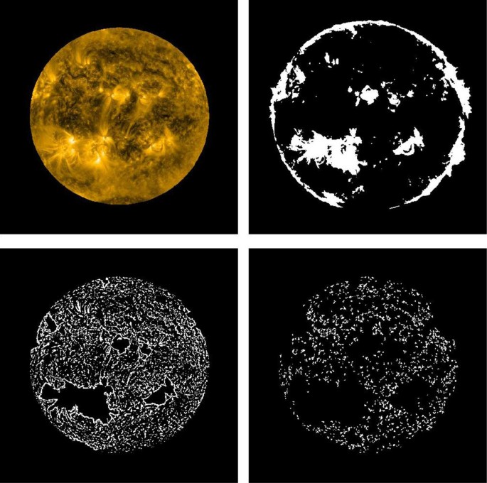

    

    Individual steps towards the BP identification. Top-left panel: AIA 193 Å image from 1 January 2012 limited to 0.95 solar radii. Top-right panel: identification of exclusion regions. Bottom-left: identification of BP candidate regions. Bottom-right: identified BPs.

• ii) Pre-processing of the image: identification of active regions

  • i) Apply a morphological opening operation (erosion followed by dilation) and then subtracting the result from the original image (‘MORPH_TOPHAT.PRO’). The erosion operator decreases the image size and removes small features. The dilation increases the image size again and fills in holes and broken areas. Overall, the opening operator removes noise and smooths the image.

  • ii) Compute standard deviation from resulting image.

  • iii) Set all pixels larger than 0.8 sigma to 1; we obtain thus a binary image.

  • iv) Apply again a morphological opening (erode followed by dilate) with a $10 \times 10$ kernel to close small holes.

  • v) A blob-coloring algorithm (‘LABEL_REGION.PRO’) numbers all regions.

  • vi) De-select all regions of a size less than 20 000 (i.e. $100\times200$ pixels). See result is visualized in Figure 8, top-right.

  • vii) The regions are classified as active regions, and are excluded from the BP identification in the next step.

• iii) Pre-select candidate regions.

  • i) Applying an edge detection algorithm by using two Gaussian filters, take the difference between the two filter results, and apply a threshold (‘EDGE_DOG.PRO’). The radii and threshold applied are 6, 30, and 12, respectively. The Gaussian filters implement blur-filters that use a Gaussian distribution to unsharp the AIA image.

  • ii) Identify all regions (‘LABEL_REGION.PRO’).

  • iii) Remove regions that are greater than 15 000 pixel, or smaller than 200 pixel. See Figure 8, bottom-left.

• iv) Identify bright points: For each candidate region identified in Step 3:

  • i) Fit an ellipsoid to the region (‘FIT_ELLIPSE.PRO’).

  • ii) Remove non-circular structures, identified by a maximum threshold for the ratio between major and minor axis (2.5), and a maximum size for the major axis of 200. The identified BPs are shown in Figure 8 bottom-right. The area of structures removed are accounted for in the quiet Sun area.

References

Alipour, N., Safari, H.: 2015, Astrophys. J. 807, 175. DOI.
Arish, S., Javaherian, M., Safari, H., Amiri, A.: 2016, Solar Phys. 291, 1209. DOI.
Aschwanden, M.J., Boerner, P., Ryan, D., Caspi, A., McTiernan, J.M., Warren, H.P.: 2015, Astrophys. J. 802, 53.
Ball, W.T., Unruh, Y.C., Krivova, N.A., Solanki, S., Wenzler, T., Mortlock, D.J., Jaffe, A.H.: 2012, Astron. Astrophys. 541, A27.
Ball, W.T., Haigh, J.D., Rozanov, E.V., Kuchar, A., Sukhodolov, T., Tummon, F., Shapiro, A.V., Schmutz, W.: 2016, Nat. Geosci. 9, 206.
Barra, V., Delouille, V., Kretzschmar, M., Hochedez, J.-F.: 2009, Astron. Astrophys. 505, 361.
BenMoussa, A., Dammasch, I.E., Hochedez, J.-F., Schühle, U., Koller, S., Stockman, Y., et al.: 2009, Astron. Astrophys. 508, 1085.
Berghmans, D., Hochedez, J.F., Defise, J.M., Lecat, J.H., Nicula, B., Slemzin, V., et al.: 2006, Adv. Space Res. 38, 1807.
Boerner, P., Edwards, C., Lemen, J., Rausch, A., Schrijver, C., Shine, R., et al.: 2012, Solar Phys. 275, 41. DOI.
Boerner, P.F., Testa, P., Warren, H., Weber, M.A., Schrijver, C.J.: 2014, Solar Phys. 289, 2377. DOI.
Carlin, B.P., Louis, T.A.: 2009, Bayesian Methods for Data Analysis, 3rd edn., Texts in Statistical Science. Chapman & Hall/CRC, Boca Raton.
Chapman, G.A., Cookson, A.M., Preminger, D.G.: 2013, Solar Phys. 283, 295. DOI.
Cheung, M.C.M., Boerner, P., Schrijver, C.J., Testa, P., Chen, F., Peter, H., Malanushenko, A.: 2015, Astrophys. J. 807, 143.
Dudok de Wit, T.D.: 2006, Solar Phys. 239, 519. DOI.
Dominique, M., Hochedez, J.-F., Schmutz, W., Dammasch, I.E., Shapiro, A.I., Kretzschmar, M., et al.: 2013, Solar Phys. 286, 21. DOI.
Dorotovic, I., Coelho, A., Rybak, J., Mora, A., Ribeiro, R., Kusa, W., Pires, R.: 2018, Sun Geosph. 13, 129.
Ermolli, I., Matthes, K., Dudok de Wit, T., Krivova, N.A., Tourpali, K., Weber, M., et al.: 2013, Atmos. Chem. Phys. 13, 3945.
Ermolli, I., Shibasaki, K., Tlatov, A., van Driel-Gesztelyi, L.: 2014, Space Sci. Rev. 186, 105. DOI.
Foreman-Mackey, D., Hogg, D.W., Lang, D., Goodman, J.: 2013, Publ. Astron. Soc. Pac. 125, 306.
Foukal, P., Lean, J.: 1988, Astrophys. J. 328, 347.
Fröhlich, C., Romero, J., Roth, H., Wehrli, C., Andersen, B.N., Appourchaux, T., et al.: 1995, Solar Phys. 162, 101. DOI.
Golub, L., Krieger, A.S., Harvey, J.W., Vaiana, G.S.: 1977, Solar Phys. 53, 111. DOI.
Goodman, J., Weare, J.: 2010, Commun. Appl. Math. Comput. Sci. 5, 65.
Haberreiter, M., Schöll, M., Dudok de Wit, T., Kretzschmar, M., Misios, S., Tourpali, K., Schmutz, W.: 2017, J. Geophys. Res. 122, 5910.
Haigh, J.D.: 1994, Nature 370, 544.
Hannah, I.G., Kontar, E.P.: 2012, Astron. Astrophys. 539, A146.
Hara, H., Nakakubo-Morimoto, K.: 2003, Astrophys. J. 589, 1062.
Haralick, R., Sternberg, S., Zhuang, X.: 1987, IEEE Trans. Pattern Anal. Mach. Intell. 532.
Hoeksema, J.T., Liu, Y., Hayashi, K., Sun, X., Schou, J., Couvidat, S., et al.: 2014, Solar Phys. 289, 3483. DOI.
Ineson, S., Maycock, A.C., Gray, L.J., Scaife, A.A., Dunstone, N.J., Harder, J.W., et al.: 2015, Nat. Commun. 6, 7535.
Kariyappa, R.: 2000, J. Astrophys. Astron. 21, 293.
Kariyappa, R., Pap, J.M.: 1996, Solar Phys. 167, 115. DOI.
Kariyappa, R., Sivaraman, K.R.: 1994, Solar Phys. 152, 139. DOI.
Kumara, S.T., Kariyappa, R., Zender, J.J., Giono, G., Delouille, V., Chitta, L.P., et al.: 2014, Astron. Astrophys. 561, A9.
Lean, J.L.: 2000, Space Sci. Rev. 94, 39.
Longcope, D.W., Kankelborg, C.C., Nelson, J.L., Pevtsov, A.A.: 2001, Astrophys. J. 553, 429.
Madjarska, M.S.: 2019, Living Rev. Solar Phys. 16, 2. DOI.
McIntosh, S.W., Gurman, J.B.: 2005, Solar Phys. 228, 285. DOI.
Nakakubo, K., Hara, H.: 2000, Adv. Space Res. 25, 1905.
Pesnell, W.D., Thompson, B.J., Chamberlin, P.C.: 2012, Solar Phys. 275, 3. DOI.
Rottman, G.J., Woods, T.N., McClintock, W.: 2006, Adv. Space Res. 37, 201.
Sattarov, I., Pevtsov, A.A., Hojaev, A.S., Sherdonov, C.T.: 2002, Astrophys. J. 564, 1042.
Sattarov, I., Pevtsov, A.A., Karachik, N.V., Sherdanov, C.T., Tillaboev, A.M.: 2010, Solar Phys. 262, 321. DOI.
Schonfeld, S.J., White, S.M., Henney, C.J., Arge, C.N., McAteer, R.T.J.: 2015, Astrophys. J. 808, 29.
Seaton, D.B., Berghmans, D., Nicula, B., Halain, J.-P., De, Groof, A., Thibert, T., et al.: 2013, Solar Phys. 286, 43. DOI.
Shahamatnia, E., Dorotovič, I., Fonseca, J.M., Ribeiro, R.A.: 2016, J. Space Weather Space Clim. 6, A16.
SILSO World Data Center: 2010 – 2020, International Sunspot Number Monthly Bulletin and online catalogue.
Verbeeck, C., Delouille, V., Mampaey, B., De Visscher, R.: 2014, Astron. Astrophys. 561, A29.
Zender, J.J., Kariyappa, R., Giono, G., Bergmann, M., Delouille, V., Damé, L., Hochedez, J.-F., Kumara, S.T.: 2017, Astron. Astrophys. 605, A41. DOI.
Acknowledgements
The authors would like to thank the PROBA2 science centre, located at the Royal Observatory of Belgium (ROB) in Brussels for providing LYRA and SWAP data taken from January 2010 to June 2020. SWAP is a project of the Centre Spatial de Liege and the Royal Observatory of Belgium funded by the Belgian Federal Science Policy Office (BELSPO). LYRA is a project of the Centre Spatial de Liege, the Physikalisch-Meteorologisches Observatorium Davos and the Royal Observatory of Belgium funded by the Belgian Federal Science Policy Office (BELSPO) and by the Swiss Bundesamt für Bildung und Wissenschaft. We also thank Solar Dynamic Observatory (SDO) of National Aeronautics and Space Administration (NASA) for providing AIA taken from May 2010 to June 2020. We thank the National Research Council and National Resources Canada for the data of the radio F10.7 cm series, and the SIDC-SILSO, Royal Observatory of Belgium, Brussels, for the daily sunspot numbers. Dr. Kariyappa would like to express his sincere thanks to ESA/ESTEC, CNRS/LATMOS and ISEE/Nagoya University (Dr. Kanya Kusano & Dr. Shinsuke Imada) for the financial support and for a detailed discussion. The authors thank Rico Landman for his advice and discussions on Bayesian statistics. The authors would like to thank the Faculty of ESA’s Science Support Office for the financial support provided. The authors appreciated the availability of the Science Support Office Computing System, the GRID, and the support given by S. de Witte. Finally, the authors would like to thank the reviewers for the constructive comments and suggestions that improved the manuscript.
Author information
Authors and Affiliations
Corresponding author
Additional information
Publisher’s Note
Springer Nature remains neutral with regard to jurisdictional claims in published maps and institutional affiliations.
This article belongs to the Topical Collection:
PROBA-2 at Ten Years
Guest Editors: Elke D’Huys, Marie Dominique and Matthew J. West