Effects of River-Ice Breakup on Sediment Transport and Implications to Stream Environments: A Review

Abstract

During the breakup of river ice covers, a greater potential for erosion occurs due to rising discharge and moving ice and the highly dynamic waves that form upon ice-jam release. Consequently, suspended-sediment concentrations can increase sharply and peak before the arrival of the peak flow. Large spikes in sediment concentrations occasionally occur during the passage of sharp waves resulting from releases of upstream ice jams and the ensuing ice runs. This is important, as river form and function (both geomorphologic and ecological) depend upon sediment erosion and deposition. Yet, sediment monitoring programs often overlook the higher suspended-sediment concentrations and loads that occur during the breakup period owing to data-collection difficulties in the presence of moving ice and ice jams. In this review paper, we introduce basics of river sediment erosion and transport and of relevant phenomena that occur during the breakup of river ice. Datasets of varying volume and detail on measured and inferred suspended-sediment concentrations during the breakup period on different rivers are reviewed and compared. Possible effects of river characteristics on seasonal sediment supply are discussed, and the implications of increased sediment supply are reviewed based on seasonal comparisons. The paper also reviews the environmental significance of increased sediment supply both on water quality and ecosystem functionality.

1. Introduction

Ice formation, growth, and breakup affect the flow dynamics of a river or stream and thus its potential for erosion and transport of sediment [1]. During freezeup, anchor ice release can remove material from the bed of a river or stream. As an ice sheet forms, the resistance to flow created by the ice cover modifies the velocity profile such as to alter flow conveyance and sediment transport. In general, erosion and the transport of sediment decrease as flow and flow velocity decrease during the winter months. However, if the flow is channelized by slush deposits under a solid ice sheet, or an ice cover is uneven (such as a reconsolidated ice cover after midwinter jamming), significant erosion and transport of sediment can occur. Nonetheless, the breakup period, characterized by increased water levels and flows, is generally more important with respect to erosion and sediment transport.

Ice breakup can be described as thermal or mechanical [2]. “Mechanical” breakup is generally a dynamic event associated with rising water levels and ice movement. Rising water levels result from increased liquid precipitation and (or) snowmelt runoff that increases the flow discharge in a river and stream and that also brings particles of fine sediment from the land surface to the watercourse. As water levels rise, the ice cover detaches from the banks, and large segments of the cover move downstream due primarily to tractive forces of flowing water on the under surface of the cover and the downslope component of the weight of ice fragments. As fragments of the ice sheet push against the river banks, they break down into smaller pieces. The scraping and or gouging of river banks by moving ice and the release of sediment during the thawing of the river bank increase sediment concentrations in the river or stream. The potential for increases in sediment concentrations is thus greater during the dynamic transient period of ice breakup than the rather less eventful midwinter and summer low-flow periods. “Thermal” breakup occurs when winter ice undergoes thermal melting and decay, thereby losing a large part of its mechanical strength and thickness before being dislodged. Relative to the more dynamic mechanical events, thermal events have limited potential for erosion and sediment transport; therefore, reference to breakup will, in the following text, refer to mechanical events unless otherwise specified.

Breakup processes can generate significant contributions to the annual sediment load, sometimes with detrimental consequences. The effects of breakup ice jams on flow conveyance and direction can increase or lessen flow velocity and tractive force, thereby leading to sediment removal or deposition, with potential localized detrimental effects with respect to the functioning of water intakes and the conservancy of aquatic habitat. Bed scour under an ice jam can have important implications with respect to pipeline and bridge pier design, as these structures can be damaged or destroyed if undermined. Javes (ice-jam-release waves) exemplify the extreme power and erosive capacity of breakup in their heights, rates of water level rise, celerities, and high speeds of associated ice runs [3]. A sharp rise in suspended-sediment concentrations occurs before the arrival of the ice run, as the leading edge of a jave propagates faster than the main body of released water. Short-duration, jave-related sediment pulses are extremely high concentrations of suspended sediment that contribute sizeable sediment loads and create a potential threat to aquatic life.

Winter ice regimes are changing in response to climatic change [4,5]. As ice processes on rivers change, e.g., greater occurrence of thermal or midwinter breakups, ice action against channel boundaries may be altered, thereby affecting channel geometry and the supply, transport, and deposition of sediment and resulting in geomorphic and ecosystem changes. The annual riverine sediment load may increase due to increased discharges and be redistributed within the seasons, with a larger percentage of the annual load during the winter [6].

The purpose of this paper is to provide a review of the effects of river-ice breakup on sediment concentrations, especially suspended sediment and its implications for water quality and aquatic life. Relevant scientific and technical background literature on sediment erosion and transport is reviewed briefly in the following section. The paper then presents an overview of ice-breakup processes followed by a summary of datasets obtained during the breakup period by several researchers, including detailed measurements in the International Saint John River (NB, Canada, and Maine, USA) and the Athabasca River (Alberta, Canada). Implications for water quality and aquatic life are discussed. In the following text, the terms “concentration” or “sediment concentration” will refer to the concentration of suspended sediment, unless specified otherwise.

2. Sediment Erosion and Transport

2.1. Bank and Bed Erosion Potential

Chassiot et al. [7] identifies several terrestrial and fluvial processes that affect bank erosion. Terrestrial processes include slow-acting preparatory processes that affect ground stability, such as groundwater seepage, freeze-thaw processes, and desiccation cycles, and more rapid, mass-wasting processes, such as debris falls and slumps. Fluvial processes include abrasive removal of bank sediment by flowing water, waves, moving ice, and highly dynamic processes associated with ice-jam release [7]. In permafrost regions and cold regions with seasonally frozen ground, progressive thawing of riverbanks in contact with flowing water results in heat transfer between water and ice that reduces particle attachment (thermal erosion), producing easily removable sediments that can be destabilized and removed by terrestrial and fluvial processes [7].

The occurrence and magnitude of bank erosion depends upon several hydraulic factors, such as flow energy, wave action, and the presence of bankfast ice, and several non-hydraulic factors, such as bank morphology, frost action, vegetation cover, and the effects of human and animal action [7]. The amount of bank erosion thus depends upon the magnitude of the forces acting on the sediment particles in a river bank and the mechanical properties of the soils, such as sediment structure, size distribution, bulk density, and mineral content, and upon the protection provided by vegetation [8].

Vandermause [9] investigated the role played by dynamic ice-breakup events in bank erosion of the Susitna River (Alaska, USA). Extensive field measurements and observations indicated that most of the bank erosion, 54 to 61 percent by sub-reach, occurs or is initiated during dynamic breakup of the winter ice cover. High water discharge in combination with ice floes and ice rubble are dominant erosion factors. Vegetated bars and terrace margins were the most susceptible to erosion, caused by impacting ice floes. Less susceptible were banks adjoining floodplain surfaces and partly protected by vegetation root mats and by shear walls of ice rubble. Bank erosion occurred less in predominantly single-channel reaches than in predominantly multi-channel reaches.

The effects of moving river ice on channel erosion and alignment have been reported, with many channels exhibiting effects of ice on channel morphology [10]. Along the gravel-bed Susitna River, Alaska, consecutive datasets of aerial photography were used to detect the location, magnitude, and timing of large-scale channel change owing to water flow and river-ice processes [10,11]. Vandermause et al. [10] examins a 2011–2015 dataset from the Susitna’s Middle River segment to quantify the extent to which bank erosion along the river is driven by river-ice or open-water fluvial processes. To determine which geomorphic surfaces and bank profiles may be more susceptible to erosion, eroded areas are examined to relate erosion extent to bank resistance, which is based on sediment composition, bank height, and vegetation. In reaches 6 and 7 of the middle stretch of the Susitna River, 41% and 7%, respectively, of the erosion occurred during a 5-day breakup period; 20% and 46%, respectively, during the start of the ice breakup though the fall period; and about 36% and 46% of the erosion could not be assigned to a timeframe during the year based on visual evidence [10]. Fluvial processes in general did not appear to cause large-scale bank retreat, although open-water erosional processes contribute to the undercutting of root-reinforced cantilevered banks by entraining non-cohesive sand and silt sediments once water levels are above the basal gravel layer [10].

Three ice-driven erosional processes were identified from field observations and analysis of aerial photography and video along the Susitna River:

• Abrasion, gouging, and removal by ice rubble of the upper layer of cantilevered rootmats thereby exposing the bank to subsequent fluvial entrainment of fine-grained material and disruption of the armour pavement of cobbles along the bank toe, with rubble-ice impact observed to be more severe for banks near the upstream tip of an island or bar or where flow directed rubble directly against a bank;
• Gouging due to the impact of moving ice floes on river banks and overtopping and bulldozing of vegetation on low islands and bars, sometimes creating pathways for flow to drain into secondary channels within multi-channel reaches;
• Increased flow velocity and the removal of armour pavement of cobbles and gravel due to ice congestion in the channel, which could occur because of an ice cover and anchor ice, flow concentration beneath and around an ice jam, and from an ice-jam-release jave. The primary effects of increased shear stress on bank erosion are mobilization of bank toe pavement (most likely due to javes), entrainment of bank material, and undercutting and failure of the vegetated top of bank [10].

Four factors that mitigate the erosive effects of ice along the Susitana River are coarse-paved bed material, bank-attached ice, vegetation rootmats, and channel form and local hydraulics [11]. Two ice-related factors limiting bank erosion are frozen banks, which limits the removal of sediments, and shear walls, which protect the bank from contact with moving ice [10].

Moving ice can erode riverbanks by grinding the bank surface, by transporting boulders, and undercutting bank materials [7,10,12,13,14]. The extent of gouging by impacting ice is less if the top of the bank has larger vegetation with protective rootmats rather vegetation with shallow rooting plants. However, ice rubble moving along the bank can shear rootmats, leaving a near-vertical bank face exposed to erosion by flows at stages above the gravel bank toe [10]. Furthermore, the effects of flow-driven rubble-ice are of greater severity where ice rubble directly impacts a bank, such as at the head of an island or bar, compared to other locations, such as the side of mid-channel islands [10].

River banks are an important source of sediment in natural streams. The annual thermal cycle is found to affect this source greatly by affecting the stability of the stream banks [15]. Gatto [8] identifies several bank erosion mechanisms that can contribute to increases in suspended sediment during the breakup period. Turcotte et al. [13] also reviews the potential effects of streambank and ice processes on sediment supply.

The occurrence and magnitude of bed erosion (i.e., scour) depends upon several factors, such as channel slope and planform, the quantity and hydraulics of channel flow (which can be affected by an ice cover), and the properties of the bed material. For non-cohesive sediment, the properties of bed material affecting scour are particle size, shape, density, and position. For cohesive bed material, the strength of the cohesive bond between the particles affects erosion [16].

The capacity of the flow to erode channel boundaries and transport sediment is related to bed shear [17]. The average bed shear stress, τ_b, is customarily expressed as:

$${\tau }_b=\gamma R_b{}^{ }{S}_f$$

(1)

where γ = unit weight of water = 9810 N/m³; R_b = bed-controlled hydraulic radius ≈ average water depth under open-water flow conditions in most rivers; and S_f = friction slope. Taking into account the Manning resistance equation, it can be further shown that:

$${\tau }_b=\gamma n_b{}^{3/2} S_f{}^{1/4} U^{3/2}$$

(2)

where n_b = the Manning’s resistance coefficient for the channel bed, and U = average flow velocity in m/s. Equation (2) is particularly helpful during ice runs because the surface velocity can be estimated by timing moving ice floes and the result multiplied by ~0.9 (per Equation (6), Section 5) to obtain average flow velocity. Noting the small exponent of the friction slope in Equation (2), reasonable estimates of the shear stress can be obtained by substituting the water-surface slope in its place. Bed shear stress can be especially high during the passage of javes because both U and S_f are considerably greater than their pre-jave values. Beltaos et al. [18] estimates a bed shear stress of approximately 120 Pa during the passage of a major jave on the lower Athabasca River, a value that was corroborated by more detailed analysis of jave characteristics [19]. By comparison, the highest known discharge in the same reach, which occurred under open-water conditions, generated an estimated bed shear stress of only 35 Pa. Erosional capacity has also been expressed in terms of unit stream power, which is defined as the product τU. Annandale [20] presents an erodibility index method based on the concept of a critical value of unit stream power that can be used to compute the hydraulic conditions under which erosion will be initiated in a wide range of materials.

2.2. Sediment Transport

Sediment is transported due to the combined effects of water flow and gravitational forces acting on the sediment. Transport modes differ depending upon sediment size, shape, and density, with larger particles sliding or bouncing along the riverbed, and finer particles suspended in the flowing water. Sediment can be transported in solution (dissolved load), in suspension (suspended load), or along the bottom of the river (bed load). Sediments transported as bed load and as suspended load have different particle size distributions, with suspended-sediment particles usually being considerably smaller than the bed-load particles. A change in land use, for example, from forest to agricultural (or logging), can substantially modify sediment transport modes and intensities in river systems by increasing fine sediment supply [21]. Many sediment transport formulae exist, but some are for total load, some are for suspended load, and some are for bed load. No formula applies to all flow and sediment conditions. Different formulae yield different results, and thus, the accuracy of results depends upon how well the formula applies to a river’s flow and sediment regime.

In gravel-bed rivers, bed load will be a major portion of total sediment load. Basically, it is possible to compute the suspended-load capacity based upon the type of bed material and the flow conditions.

In-stream sediment transport depends on the sediment supply and the sediment transport capacity [13]. Sources of suspended sediment during breakup include particulate material deposited by wind on the ice cover prior to breakup, sediment carried by runoff from land surfaces, material removed from the banks by freeze-thaw cycles, and the bed and bank soils eroded, abraded, or gouged by moving ice and water. A portion of the suspended sediment in a river (such as clays) may be so fine that the particles do not rely on turbulence but are kept in suspension by thermal molecular agitation (Brownian motion) and are referred to as wash load, as it washes through the system [22]. If the sediment supply is limited, the actual sediment loads will be less that the sediment transport capacity of the stream. The concentration of suspended sediment is generally several orders of magnitude below the channel’s capacity for sediment transport [23]. Therefore, the rate of supply is the dominant control on suspended-sediment concentration. Considerable scatter is evident when the concentration of suspended sediment is plotted against discharge. Temporal changes in suspended-sediment concentrations with hydroclimatic conditions may create a hysteresis loop because the rate of fine sediment supplied to the flow is greater during the rising limb of the hydrograph compared to the falling limb [24]. Sediment deposited and stored on the channel bed between storms is entrained by the increasing velocities during the rising limb, leaving less sediment supplied to the flow during the falling limb [23].

The suspended load transport per unit width is computed by integration over the flow depth of suspended-sediment concentration times the local mean longitudinal flow velocity. Integration of this load across the entire channel width results in the total suspended load, which often dominates total sediment flux, and is thus a major contributor to sediment influx to lakes and oceans and to deposition onto floodplains.

The particle fall velocity and the sediment diffusion coefficient are the main controlling hydraulic parameters for the suspended load [25]. Initiation of sediment suspension from the riverbed begins when the turbulent eddies have dominant vertical velocity components that exceed the particle fall velocity. The maximum value of the vertical turbulence intensity is of the same order as the bed-shear velocity [25]. The particle fall velocity is a function primarily of the kinematic fluid viscosity, sediment-specific gravity, and the representative particle diameter of suspended sediment. Different equations for particle fall velocity have been proposed for different ranges of sediment size. The sediment diffusion coefficient governs the concentration profile of suspended sediment [26]. Temperature variations impact rivers that transport a preponderance of fine sediment, a characteristic of many large rivers [27]. River temperature controls fluid density and viscosity and hence sediment transport.

Total suspended solids (TSS) and turbidity are often used as indicators of suspended sediment. TSS is a direct measurement of quantity of solid material, both organic and inorganic, per volume of water. Although SSC (suspended sediment concentration) and TSS are both measurements of the solid-phase material within a water column, values of TSS and SSC can differ due to different laboratory procedures used in their determination. Turbidity is a measurement of the passage of light though a liquid, which often can be measured or qualitatively observed onsite. Turbidity can be affected by solid and dissolved substances. Mean turbidities of ice-covered river water of the Kokemäenjoki River, Finland, were observed under similar discharges (<300 m³/s) to be 1.5 to 3.3 times less than during summer or winter ice-free conditions [6]. TSS can be used to calculate sedimentation rates, while it is generally considered that turbidity cannot (e.g., [28]). In general, SSC, TSS, and turbidity data collected from natural water are not directly comparable and should not be used interchangeably.

2.3. Sediment Transport during an Ice Season

Lower streamflow during winter periods occurs due to limited surface runoff during cold weather. Mid-winter flow velocities are relatively low under a stable ice cover, thereby lowering bed shear and associated sediment transport. TSS and shear stress analyses of the Kokemäenjoki River, Finland, indicate that the sediment transportation in the river declines under ice cover [6].

Anchor-ice-rafting can have a major role in moving bed sediment, as anchor ice released from the bed can transport some bed sediment to which the ice was attached. Based on field observations and measurements in the Laramie River, USA, Kempema et al. [29] found anchor-ice-rafted sediment is coarser than fluvially transported bedload sediment; that is, ice rafting (not peak spring flows) transported the largest particles. The amount of sediment transport by anchor ice could be significant in some regulated rivers where open water persists throughout the winter season, letting anchor ice form and release often [30]. For three regulated rivers in Alberta, Canada (the North Saskatchewan, Peace, and Kananaskis rivers), the average sediment concentration contained in released, floating anchor ice was found to be 28.2 g/L with a standard deviation of 33.2 g/L and a median of 18.4 g/L [30].

The ice cover itself can also contain sediment during the ice season. High flows at freezeup coupled with irregular winter flows are observed to result in sediment embedded in the ice of both the Athabasca and Peace River systems [31]. Ice-entrained sediment can be transported downstream with broken ice during breakup and enter the water column as the ice melts.

For the Tanana River near Fairbanks, Alaska, Lawson et al. [32] reported a lower ratio of suspended-sediment load to bed load during the winter (February–March 1984) compared to the summer. Measured SSC values during the period of ice cover were 51 mg/L to 152 mg/L, considerably higher than the winter pre-breakup SSCs reported by [33,34]. Possible reasons for this are finer bed and bank material and increased velocities in slush-confined channels under the solid ice cover. This shows that suspended-sediment concentration is dependent upon local conditions.

Using a numerical model to evaluate the effects of various parameters on shear stresses during ice motion, Ferrick and Weyrick [35] found the amplitude of increase in suspended-sediment-transport capacity increased with ice velocity and acceleration and decreased with relative ice roughness. Higher initial energy gradients led to smaller increases in sediment transport capacities than in flow velocity [35].

3. Overview of Ice Breakup Processes

3.1. Physical Processes

The breakup is typically a brief event spanning the transition from the relatively complete and integral winter ice cover to the open-water condition. Often attended by rapid increases in river stage and flow velocities, the breakup of river ice can disrupt ecosystems, abrade stream banks, alter channel morphology, scour riverbeds, and transport large quantities of sediment and associated contaminants, and modify water quality. Detailed background information on breakup processes and their socio-economic and environmental impacts can be found in the book River Ice Breakup [2].

Ice breakup is triggered by mild weather, which can generate snowmelt and rainfall on the one hand and, on the other hand, thermally degrade the stationary winter ice over. As river flow increases, so do the hydrodynamic forces that are applied on the ice cover, while the rising water levels reduce ice attachment to the river banks and bed. At the same time, the ice cover becomes more susceptible to dislodgment and fracture via thermally induced reductions in thickness and strength. Eventually, large segments of the fragmented cover are dislodged and mobilized by the flow. This is the onset of breakup and is followed by the drive, i.e., the transport and further breakdown of large ice sheets into smaller blocks and rubble. The onset is governed by many factors, including channel morphology, which is highly variable along the river. It is thus common to find reaches where breakup has started alternating with reaches where the winter ice cover has not yet moved.

Invariably, this situation leads to jamming because ice blocks moving down the river in one reach encounter stationary ice cover in another reach and begin to pile up behind it, initiating a jam, which can be tens of metres or, more often, several to many kilometres long. Ice-jam residence times vary from a few minutes to many days depending on a variety of factors, such as local channel morphology and bathymetry, variation of discharge (increasing, steady, decreasing), and rate of thermal degradation of the intact ice cover downstream of the jam (air temperature, precipitation, solar radiation, cloudiness). The jave that is generated by an abrupt release of an ice jam can dislodge and break up long sections of intact downstream ice. On occasion, the stationary ice is too strong or the jave too attenuated, and the ice run that lags behind the jave is arrested, forming a new jam. In this manner, more and more ice is broken up and carried down the river until the final jam releases. This is the start of the wash or final clearance of ice from a river reach, though grounded remnants of ice rubble and ice slabs may linger for weeks.

In the colder continental parts of Canada, such as the Prairies or Territories, we are most familiar with a single event, the spring breakup, which is triggered by snowmelt. In more temperate regions, however, such as parts of Atlantic Canada, Quebec, Ontario, and British Columbia, events called mid-winter thaws are common. Usually occurring in January or February, they consist of a few days of mild weather and often come with significant rainfall. River flows may rise very rapidly and sufficiently to trigger breakup on many local rivers. This is the mid-winter breakup, which can be more severe than a spring event because of the sharp rise in flow that results from the rain-snowmelt combination. Moreover, dealing with the aftermath of flooding is hampered by the cold weather that resumes in a few days, while many mid-winter jams do not release but freeze in place, posing an additional threat during subsequent runoff events.

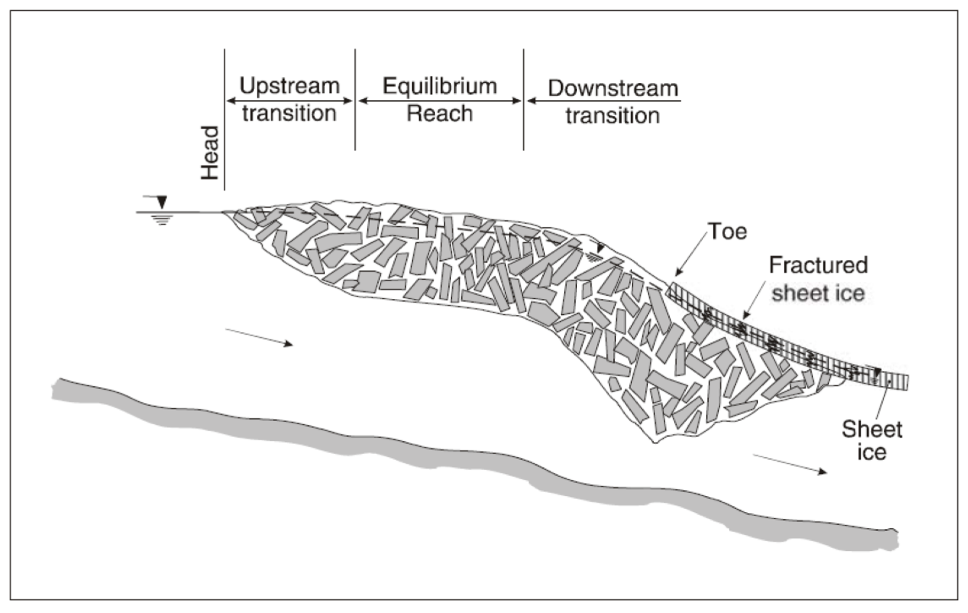
Ice jams and javes are the primary breakup phenomena that contribute to erosion, deposition, and transport of sediment. Owing to their large aggregate thickness and underside roughness, major ice jams raise water levels far above what would suffice to pass the prevailing flow under open-water conditions. This can lead to flooding and deposition of large quantities of sediment on river floodplains. Typically, the longitudinal profile of an ice jam (Figure 1) entails the potential for bed scour, primarily near the toe, where significantly increased velocities and shear stresses are encountered owing to the reduced under-ice flow area. It is evident in Figure 1 that as the flow approaches the toe of the jam, the associated bed shear stress will develop a positive longitudinal gradient followed by a negative gradient farther downstream. If the magnitude of the shear stress is sufficient to erode the bed, scour will occur upstream and deposition downstream of the toe location. To a lesser degree, the same may occur immediately downstream of the head of the jam, where a positive shear stress gradient is also likely to develop. Upstream of the head, the relatively large water depth is associated with smaller flow velocities and shear stresses, which decrease in the downstream direction. Here, sediment deposition will likely occur depending on the magnitude and particle size of any incoming sediment, be it suspended or bed load.

The blockage and large hydraulic resistance to flow created by ice jams can divert flow away from the main channel and into secondary channels. As a result, local flow velocities may increase far beyond what is expected under non-jammed conditions. Gerard [37] observed ~3 m high standing waves in a side channel of the Athabasca River at Fort McMurray following partial failure of an ice jam on 22 April 1974. From crude estimates of the wave length, he estimated the flow velocity to have been between 4 and 7 m/s. The partial failure had “concentrated the total release into a small side channel near the left bank”.

Typically, ice jams release abruptly as a result of increasing river flow and/or weakening of the downstream stationary sheet-ice cover. If the toe of the jam happens to be grounded, ice blocks in contact with the channel boundary could gouge the riverbed and banks, changing local morphology and releasing large amounts of sediment into the flow [38]. Moreover, a release generates a positive and a negative wave, respectively, moving in the downstream and upstream directions. The rapid decrease in water levels upstream of the toe of the jam can cause extensive bank failure due to pore pressure imbalance. However, it is the sharp positive wave, or jave, that is much more dynamic than a runoff wave and can cause the bulk of sediment erosion and transport. Early work on javes was discussed in the comprehensive review and synthesis by [39]. More recent research further elucidated jave characteristics, including but not limited to [3,40,41,42,43].

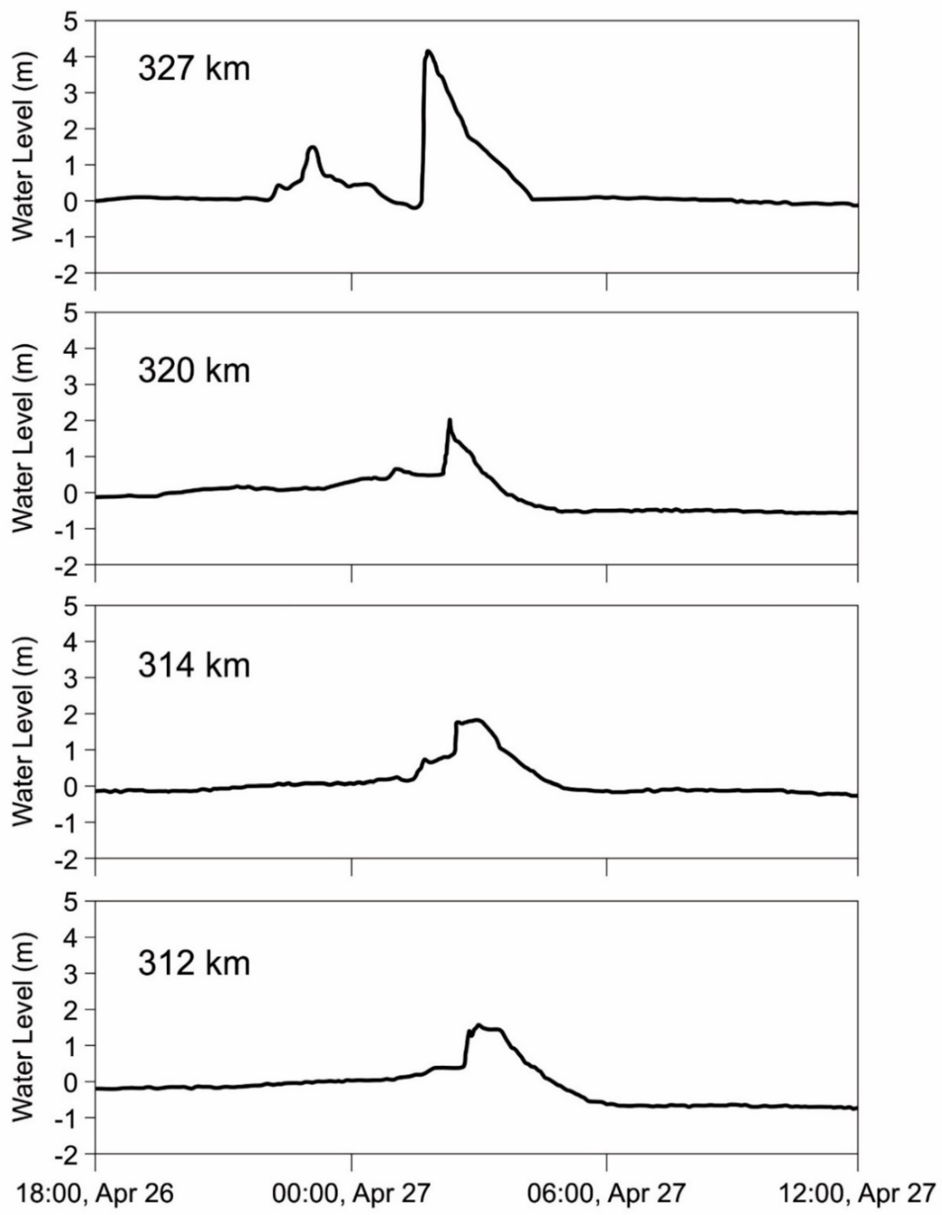
Examples of jave waveforms are illustrated in Figure 2. The rise to the peak stage lasted 15 min in total, but the first 5 min brought about a rise of ~4 m at the farthest upstream station [41]. This extreme rate of rise is one of the highest known to date. Comparable rates of rise have also been recorded in the Restigouche River (~3 m in 6 min; [44]) and the Athabasca River (~4.5 m in 6 min; [18]).

Theoretical considerations suggest that the leading-edge celerity of a jave should not exceed the celerity of a gravity wave, C_g, or be less than the celerity of a kinematic wave, C_k, [3,43,45]. The theoretical celerities are defined as:

$$C_g\approx U_o+\sqrt{g{h}_o}$$

(3)

$$C_k\approx \beta U_o$$

(4)

in which U_o and h_o = pre-jave mean flow velocity and depth, respectively; g = gravitational acceleration; and β = coefficient equal to 3/2 or 5/3 depending on whether the Chezy or the Manning equation is used to relate velocity to hydraulic radius and friction slope. Observations on the Hay River, NWT, Canada, showed that the leading-edge celerity remained close to C_g for at least 1.1 to 2.9 ice-jam lengths of travel, with the crest celerity being a fraction of C_g [43]. Beyond this distance, both celerities decreased, with the crest celerity approaching C_k.

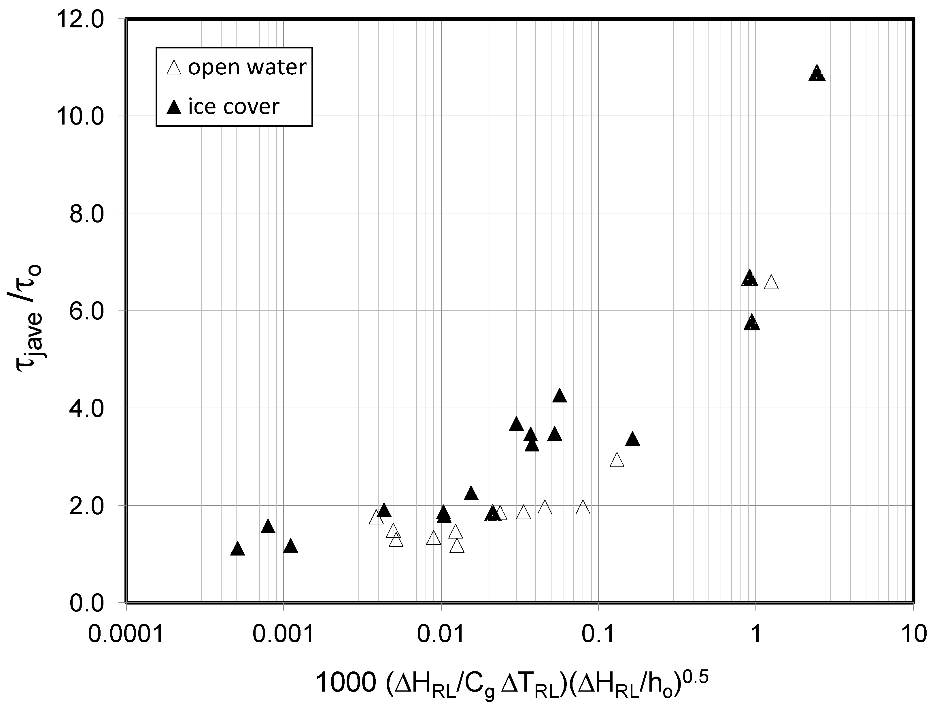
The presence of moving ice renders problematic the measurement of velocity and discharge. However, such hydrodynamic variables, including the bed shear stress, can be inferred using the Rising Limb Analysis Method (RLAM), developed by [46]. Application of the RLAM to numerous recorded waveforms has revealed that javes can greatly amplify hydrodynamic variables especially where the wave height is large and the rising limb brief, as illustrated in Figure 3. The scatter is due to partial only accounting of the several independent variables arising from dimensional analysis; therefore, Figure 3 provides estimates of magnitude range rather than a single value of the amplification ratio. For a moderately sharp jave, rising 3 m in 30 min, with initial flow depth and velocity of 3 m and 1 m/s, respectively, the value of the abscissa works out to be 0.26, indicating a four- to six-fold amplification. For waves propagating under a stationary ice cover that is dislodged prior to the wave crest, the quantity τ_jave may be less than the peak shear stress because the open-water flow condition can generate higher shear than what RLAM calculates, assuming stationary cover throughout the duration of the rising limb [19]. Therefore, the amplification ratios indicated by the solid triangles in Figure 3 may be equal to or greater than the actual peak values generated by the respective javes.

Beltaos et al. [47] and Beltaos [19] reported bed shear stresses of up to 40 and 140 Pa generated by javes in the Saint John and Athabasca Rivers, respectively. The higher value occurred very near the toe of the released jam and likely represents the highest that occurred along the river during the passage of that jave. Though the corresponding breakup events were of the dynamic kind, neither one was extreme.

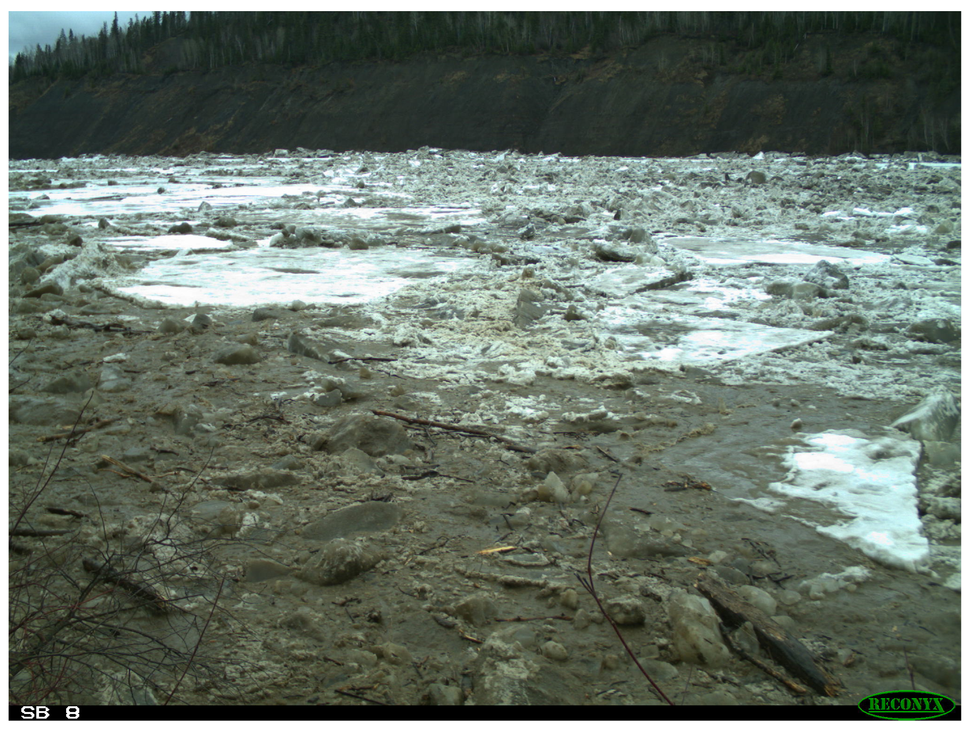
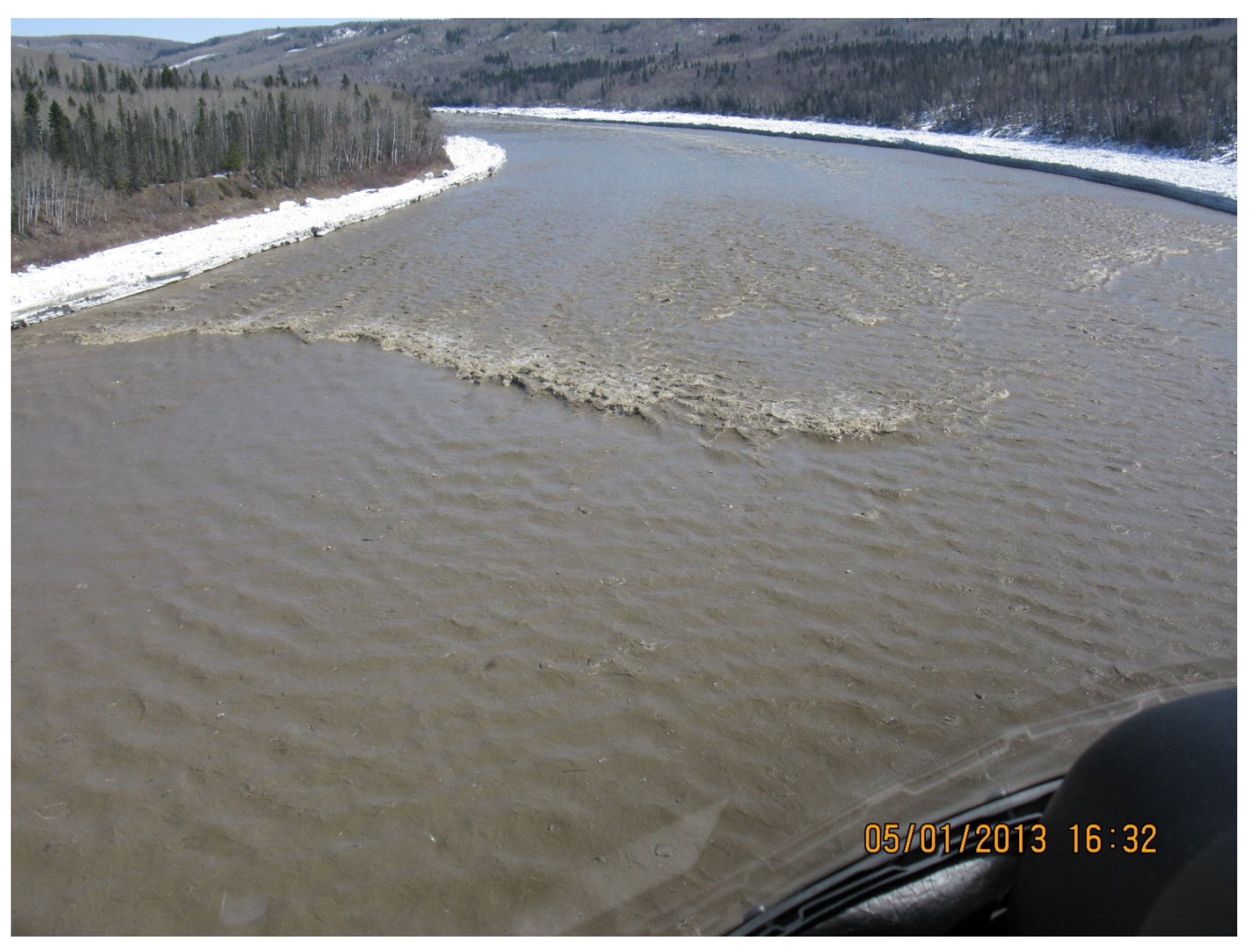
High velocities and shear stresses suggest potential for intense bed and bank erosion as well as transport of large quantities of sediment both as bed and as suspended load. Visual evidence indicates that the water takes on a deep muddy hue when a river opens in dynamic fashion, as in the case of a jave. River conditions near the Fort McMurray golf course were characterized by a deep muddy hue shortly after the arrival of a jave and dislodgment of the winter ice cover (Figure 4). At this early phase of the ice run, most of the river surface is covered by ice plates and rubble. However, the surface of the water and various churning ice blocks in it can be seen in the lower left corner of the photo; its colour suggests a very high concentration of suspended sediment. Over time, concentrations gradually decrease, but elevated values linger (Figure 5).

Numerous field observations and related data analysis (e.g., [3,43,44]) have conclusively shown that the rising limb of the jave advances at a greater rate than the ice run, which comprises rubble from the released jam. Typically, a jave advances at first under stationary ice cover, which is often mobilized at some point along the rising limb; large ice sheets then pass by for a relatively brief time, followed by bank-to-bank ice rubble. This sequence has additional implications to erosional processes, namely:

(i)

Swiftly moving large ice sheets that follow dislodgment of the stationary ice cover can scrape and gouge riverbanks over extended channel distances.

(ii)

Heavy runs of ice rubble that follow the large ice sheets often result in formation of thick grounded strips along the river banks. Such strips shield the banks from further erosion either by ice abrasion and gouging or by the high-velocity water underneath the moving rubble.

3.2. Sediment Transport Modelling in Ice-Laden Rivers

Numerous laboratory experiments in channels with stationary covers of constant thickness have shown that bed sediment transport equations previously developed for open-channel flow can be suitably modified for under-ice transport [12]. Knack and Shen [48,49] further developed such equations and incorporated them in a hydrodynamic model, which successfully simulated laboratory scour and deposition experiments under conditions of steady incoming flow.

Bed sediment transport under the highly dynamic flow conditions that prevail upon and after release of ice jams is examined by coupling a non-hydrostatic 3D hydrodynamic model with bed erosion and deposition equations to track the changing bathymetry of a riverbed [50]. Initially, an ice jam was modelled as a rigid body of water near the free surface that constricts the flow. This “jam” did not exchange mass or momentum with the stream, but the “ice” body could have a realistic shape and offer resistance to the flow of water through the constriction. The release was modelled by suddenly enabling the “ice” to flow and exchange mass and momentum with the water. This model was applied to the extreme 1984 ice jam event in the St. Clair River to determine whether bed scour could have occurred. The simulations suggested that events like the 1984 ice jam can cause significant scouring of the St. Clair River bed upon their release, and the authors recommended future field research to ascertain this result.

Dynamic changes in the state of the pre-release stationary ice cover, which is typically located downstream of an ice jam and is often mobilized and broken up by advancing javes over long distances, add complexity to numerical simulation. The Knack and Shen model [48,49] can simulate flow hydrodynamics under such conditions and hence compute bed sediment transport, but this capability has not yet been tested, owing to lack of relevant data (Dr. I. Knack, pers. comm., March 2021, [51]).

Field observations and data [52,53] suggest that a large component of the sediment load being delivered during breakup derives from bank erosion processes. Although bank erosion rates have been quantified by numerous investigators for open-water flow conditions [54], this knowledge has not yet been incorporated in hydrodynamic river-ice models.

4. Suspended-Sediment Concentrations Shortly before and during the Breakup Period

Measurements of SSCs and sediment characteristics during the pre-breakup and breakup periods are discussed in this section, based on a review of literature. During the breakup of river ice covers, rising discharge and moving ice increase the potential for erosion due to rising discharge and moving ice. The bulk of the sediment load is thus delivered on the rising limb of the flow hydrograph, evincing constraints on the amount of sediment supply.

Prowse [33] reported measurements and analyses of SSC during the 1987 pre-breakup and breakup periods on the Liard River near its confluence with the Mackenzie River. All sampling was done 300–500 m from the left bank in an approximately 700-m wide reach used by the Water Survey of Canada to monitor discharge and sediment of the lower Liard River (hydrometric station No. 10ED002, Liard River near the Mouth, drainage area = 275,000 km²). Up until 26 April, SSCs remained below 10 mg/L but then began to steadily rise as breakup occurred upstream and along tributaries. Measurements made on 1 May from a helicopter during the ice fracturing and fragmenting period revealed a sediment concentration of 70 mg/L. The general rise in SSC prior to breakup at the sampling site is probably attributable to a rise in velocities and discharge and additional sediment contributions from upstream tributaries, including some more southern rivers which break up earlier [33]. Ice cleared the reach on 2 May, and a local, small jam occurred downstream, increasing water levels in the sampling reach. A sample on 4 May revealed that the sediment concentration had risen to approximately 120 mg/L. The highest measured SSC during the 1987 breakup of approximately 1067 mg/L occurred on 6 May during release of jammed ice remaining on the lower Liard [33]. This value far exceeded normal sediment concentrations for open-water conditions with equivalent discharge and was closer to annual peak-sediment concentrations recorded at two to five times greater discharge. Upstream ice-induced erosion is most likely responsible for the rapid increase during the 4–6 May breakup period [33]. Higher sediment concentrations could be produced by more dynamic breakup events than the moderate 1987 event, which was characterized by a nonuniform downstream breakup progression typical of a thermal breakup.

Milburn and Prowse [55] presents data from a 1993 sampling program on the Liard River and further discusses the results of suspended-sediment sampling conducted in 1987. During both the 1987 and 1993 data gathering, samplers were lowered through holes in the ice during pre-breakup and from a helicopter positioned over leads during active breakup. The 1987 breakup stage and the 1993 breakup stage were just below and above the maximum open-water stage, respectively, and are more representative of average than extreme breakup severity. In both years, suspended-sediment concentrations remained below 10 mg/L two weeks before breakup but then rose by an order of magnitude prior to breakup. This increase in pre-breakup suspended sediment could be due to resuspension of fine-grained sediment deposited during the low-flow winter period [55]. As reported in [33,56], SSCs in 1987 rose more as breakup progressed, reaching a maximum of 1067 mg/L with a concurrent mean daily discharge of 2550 m³/s. The 1987 high SSCs could be related to an upstream release of an ice jam. In 1993, SSCs rose to 291 mg/L (at 2280 m³/s) just before breakup and peaked at 331 mg/L (at 2480 m³/s) during the final ice run [55].

The average proportions of clay, silt, and fine sands in the five samples collected in 1987 just before and at breakup are 18, 66, and 16%, respectively; they are much finer than that when measured during the open-water period [55]. The high percentage of very fine material in these samples supports remobilization of over-winter accumulated sediment material as a source of pre- and early breakup suspended sediment. If particle-size analysis had continued later during breakup, it is expected that later samples would show a shift toward higher percentages of fine sand fractions because of increased erosive action [55].

Measured sediment concentration in the Hequ Reach of the Yellow River, China, increases with flow discharge and during ice breakup, while the grain size distribution of sediment can show seasonal variations [57]. The suspended load carried by the flow during the winter is coarser than that during formation of ice jams and the breakup period, as the supply of finer sediment from land sources is reduced, and some finer sediment is entrained in ice, therefore making the coarser material of the riverbed the predominant source of sediment [57].

Toniolo et al. [58] reports on field measurements carried out during the spring breakup of 2011 on seven pristine streams located in the National Petroleum Reserve in Alaska. Estimates of the Shields parameter indicated finer sediments could be moved in suspension but that coarse sand would move as bedload. The highest SSC of 186.55 mg/L reported in the paper occurred on 2 June on the Fish River, and the corresponding suspended-sediment load was estimated to be nearly 14.9 kg/s. Suspended-sediment concentrations more than 125 mg/L were also reported for the Seebee Creek and Prince Creek. In general, changes in suspended-sediment concentrations can be associated with variations in discharge and with moving ice.

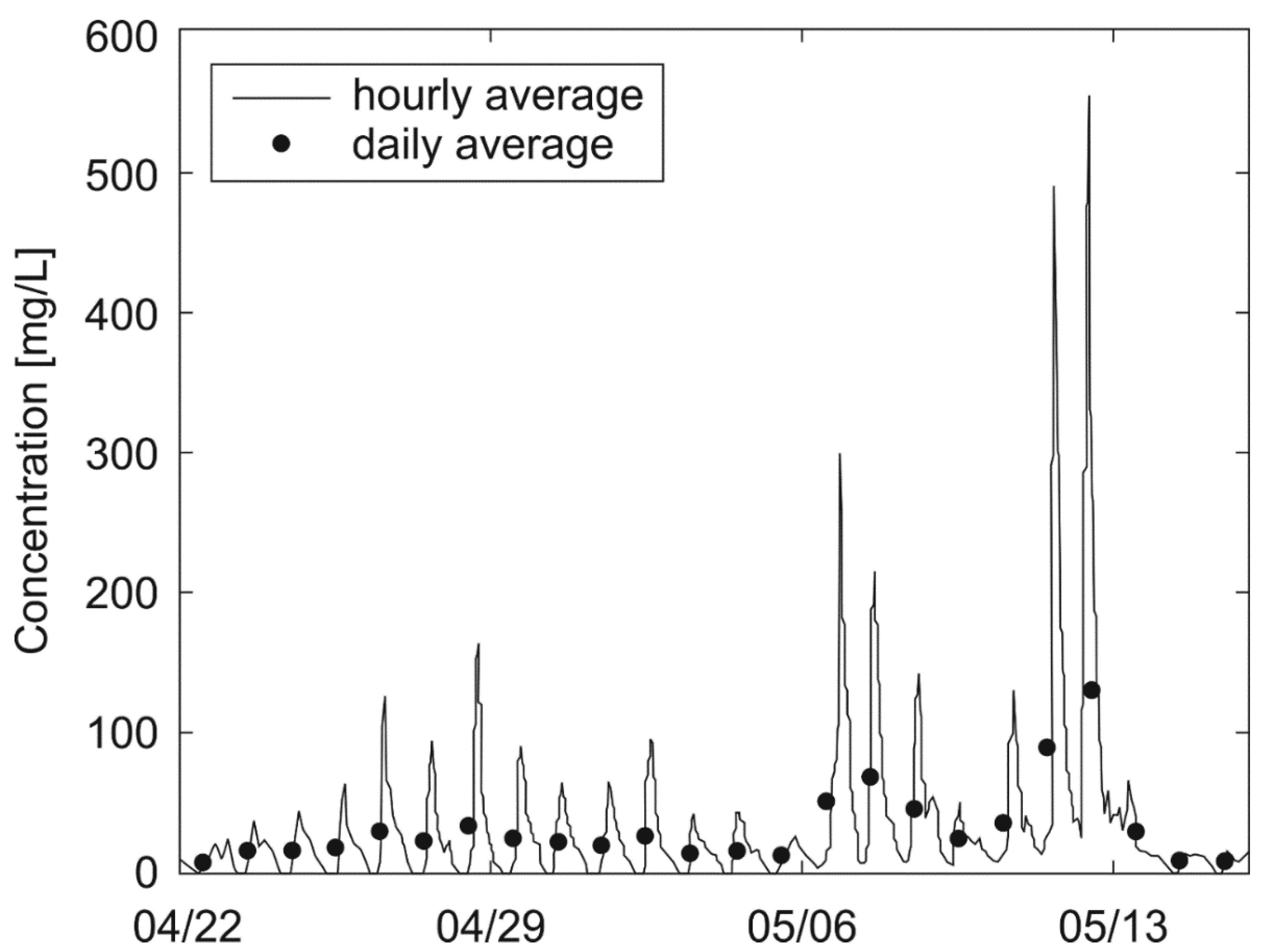
Moore et al. [59] presents hourly and daily-averaged SSC values on the Nelson River, Manitoba, estimated from acoustic data during hydropeaking operations at the Limestone Generating Station. Daily-averaged SSCs increase from around 7 mg/L to 130 mg/L during the breakup period. Suspended-sediment concentration is observed at breakup to reach 10 times SSC values under a stable ice cover [59]. Hourly average peak values of SSC were much higher, attaining ~550 mg/L on one occasion (Figure 6).

Environment Canada and the New Brunswick Department of the Environment (NBDOE) undertook a joint five-year study (1993–1997) of ice breakup and jamming along the Saint John River (SJR) from the Dickey area in Maine, United States, to St. Leonard, New Brunswick, Canada. Sediment-related aspects of the study, including methodology and findings, are presented in Beltaos and Burrell [34,52]. The main findings are summarized in the next few paragraphs.

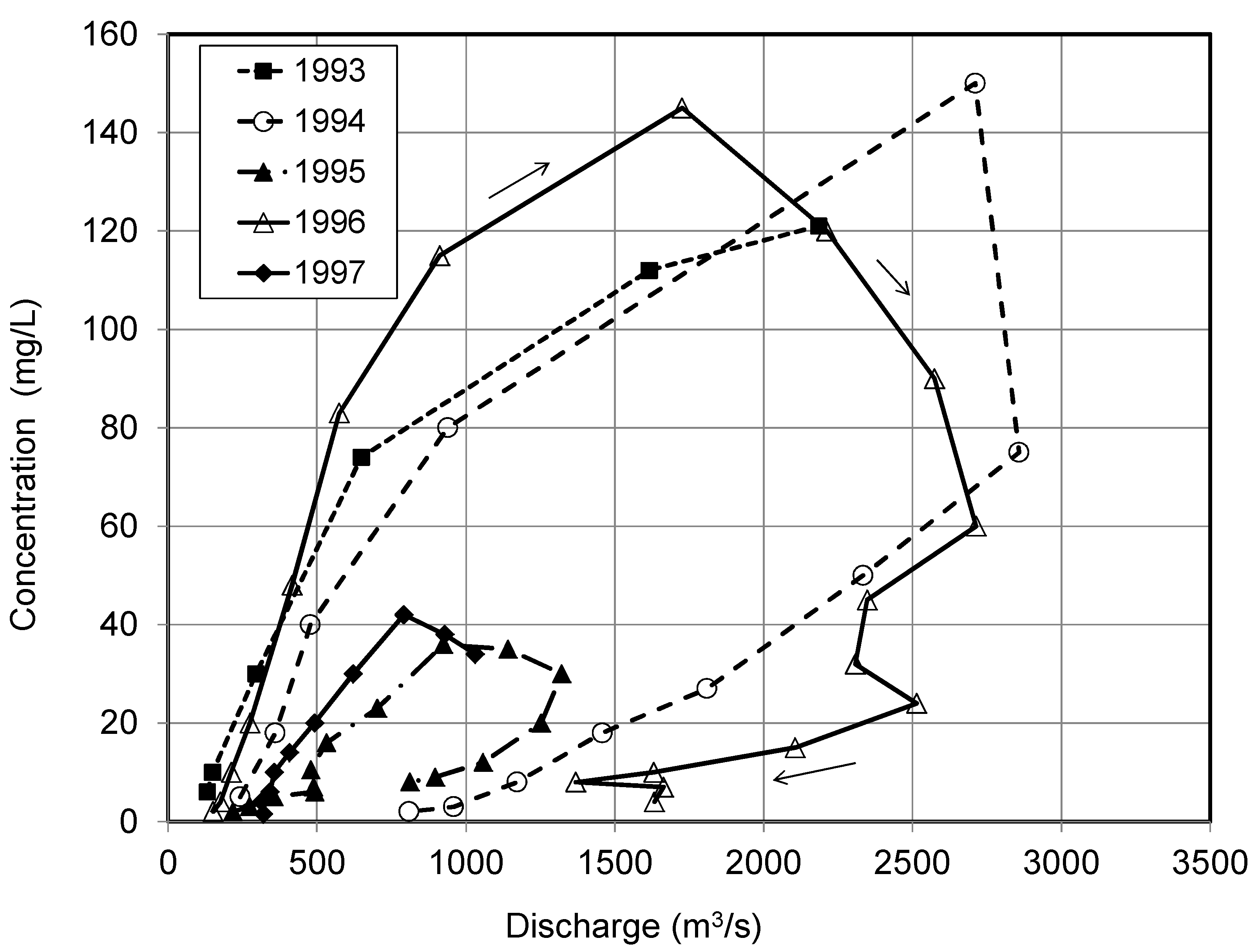
The temporal and spatial variation of the SSC was investigated by acquiring and analysing suspended-sediment samples at four bridges along the Saint John River from Dickey, Maine, USA to Saint-Leonard, New Brunswick, Canada [34,52]. Using the bridges as platforms, samples were acquired by dipping standard 750-mL glass bottles into the river or inserting them in a P72 point-integrating fish-type sampler. During typical freezeup conditions, measured SSCs along the Saint John River ranged from 0 to ~2 mg/L [34]. Concentrations increased on occasion, when the freezeup process was interrupted by small runoff from minor rain-on-snow events, decreasing again as the flow subsided. Similar values of SSC (~0 to 2 mg/L) were also found during steady-flow conditions in the winter right up to late March and even in the first half of April [34]. Peak runoff-induced sediment concentrations during the 1993- to 1997-inclusive breakup events ranged from ~35 to 150 mg/L (Figure 7), much greater than under open-water conditions. As described in Section 4, even higher SSCs were measured during brief sediment “pulses” accompanying the passage of javes. The suspended-sediment loads associated with breakup events can be the greatest fraction of the total annual loads [34].

The SSCs gradually decrease as river flow decreases and water levels subside; however, SSCs were found to decrease to pre-event values much faster than does discharge, with the peak discharge lagging 1–3 days later than the peak SSC, thereby indicating a limit on available sediment supply during the breakup event. In many rivers, such as the Saint John River, the rate of sediment supply rather than the flow capacity limits the amount of sediment transport. The hysteresis loop in the sediment rating curve of SSC versus discharge (Figure 7) is an indication of limits to sediment supply. The relationship between suspended-sediment loads and flow discharge can also vary depending upon the type of hydroclimatic event and its intensity. Though concentration–discharge relationships involve large scatter, sediment loads delivered during specific runoff events correlated well with corresponding water volumes [34].

Using a laboratory Malvern laser particle-size analyser unit, many dip samples obtained during the 1993 breakup along the Saint John River were analysed to determine primary particle sizes during the actual breakup event. Each sample was first hand shaken and analysed and then sonicated to destroy any flocs that might have been present and analysed again [52]. Results indicate that primary sediment particles in suspension are orders of magnitude finer (D₅₀ ~ 10 μm on average) than the river bed material, suggesting that the bulk of the suspended sediment does not originate from the bed of the river. The strongly looped appearance of C vs. Q graphs (Figure 7) supports this finding.

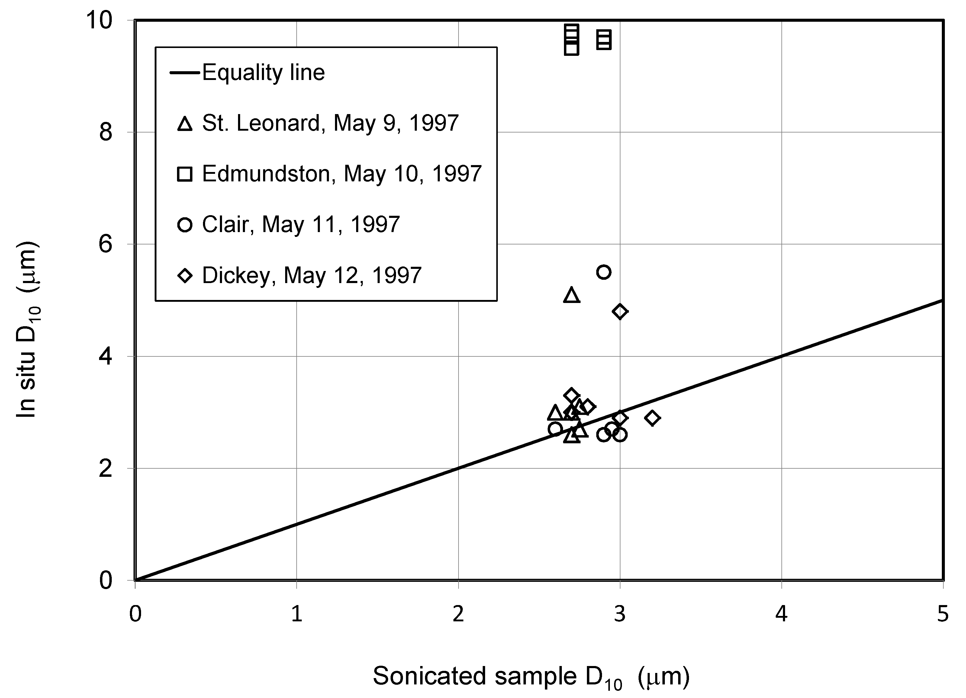
To investigate whether flocculation occurs in the river environment, a field Malvern unit was deployed at two bridge sites (Edmundston, St. Leonard) on 24 August 1993 (flow ~75 m³/s) and at four bridge sites (Dickey, Clair, Edmundston, and St. Leonard) in May 1997 (flow ~1500 m³/s). During the August 1993 measurements, D₁₀, D₅₀, and D₉₀ showed little lateral variability with average values of ~4, 14, and 35 μm, respectively, while the May 1997 results indicated greater variability along and across the channel (D₅₀ ~11 to 29 μm). Comparison with corresponding sonicated samples indicated significant flocculation at the higher flow condition (Figure 8). The presence of moving ice precluded deployment of the field Malvern unit during breakup conditions. Indirect evidence suggests that flocculation may be even more intense during breakup [52].

For the Lower Athabasca River, a positive correlation was found between SSC and flow discharge using sediment data for the WSC (Water Survey of Canada) hydrometric gauge located a few km downstream of Fort McMurray [60]. The WSC data set, which consists of published daily values of sediment load during the years 1969–1972, exhibits large scatter, which can be largely enveloped by the relationships [19]:

$$Load=7\times {10}^{-6}{Q}^3\mathrm{to}5\times {10}^{-5}{Q}^3$$

(5)

in which the load is expressed in tonnes per day, and Q = flow discharge in m³/s. Since the load equals Q × SSC, it can be shown via Equation (5) that SSC (in mg/L) would range from 8 × 10⁻⁵ × Q² to 7 × 10⁻⁴ × Q². For typical breakup flows at this location (~500 to 1000 m³/s), SSC values of 20 to 700 mg/L should be common; they can be much larger during the passage of javes, when discharge can be several times the pre-jave value.

Skolasińska and Nowak [61] analysed data collected at the Sieradz gauging station (hydrometric basin area =8156 km²) in Central Poland during the period of 1961–1980 and found that changes in SSC on the Warta River occurred during periods of river ice. Suspended-sediment concentrations increased gradually during freezeup and increased rapidly when the ice cover broke, during which time ice movement caused lateral erosion of the river banks [61]. From the data presented in the paper, the suspended-sediment concentration seems to have exceeded 70 mg/L during the breakup period.

5. Javes and Sediment Pulses

As discussed in Section 3.1, the highly dynamic jave is a wave form that occurs in ice-forming rivers and can cause significant bed scour and bank erosion. Examples of jave observations are presented in this section along with observed jave celerities and concomitant SSCs. Observations and data on a jave that occurred on 26 April 2002 on the Athabasca River were reported in [62]. Upon jam release, the water level just downstream was observed to rise 4.4 m in 15 min as the jave passed, and jave celerity in the reach was estimated to be 4.05 m/s, decreasing as it moved downstream). The peak ice concentration was observed to lag the crest of the wave as it travelled downstream [62]. Beltaos and Burrell [44] reports on field observations and measurements of three javes on different New Brunswick rivers. The passage of the jave created upon the release on 13 April 2002 of an ice jam in the Saint John River (toe 7.8 km upstream of Clair) was evident in the output of a pressure logger, installed 900 m downstream of the toe and at two downstream hydrometric stations (Fort Kent and Edmundston). An inspection of the data revealed that the celerities of the jave leading edge, peak stage, and trailing edge differed [44]. Between the surge meter and the Fort Kent gauge (distance of 8.2 km), the celerity of the leading edge and the celerity of the jave peak were 5.5 m/s and 2.5 m/s, respectively. For the stretch of river from Fort Kent to Edmundston (distance of 34 km), the celerities of the leading edge, peak, and trailing edge were 3.5 m/s, 2.1 m/s, and 1.7 m/s, respectively [44]. A review of historic records of several ice-jam release events on the Athabasca River at Fort McMurray, Alberta, indicates that release waves more than 3 m in height and propagation speeds in excess of 4 to 5 m/s were common [41]. Factors affecting jave propagation speeds were the interaction of water and ice within the jam, the size of the wave upon release, the distance travelled, channel geometry, downstream ice conditions, and the temporally jamming and re-release of released ice [41]. Detailed documentations of several large javes in the Hay and Athabasca Rivers are presented in [43] and [18], respectively.

The bed shear stress, which quantifies the erosive power of the flow, was deduced from measured waveforms using the RLAM and shown to be considerably amplified during the passage of a jave. Peak values of ~40, 100, and 140 Pa were reported for javes in the Saint John, Restigouche, and Athabasca Rivers, respectively [3,19]. Erosive power is also manifested in water velocity, which can be visually estimated by timing various ice floes in ice runs. Ice velocities of 3 m/s are common [3]. Ice run speeds ranging from 2.5 to 4.2 m/s during the 2007 breakup event on the Athabasca River above Fort McMurray were reported in [42]. Notably, extreme ice speeds have been reported in this area over the years, the highest being 7.4 m/s [63]. Ice speeds of ~5 m/s in the same area and loss of two pressure loggers as a result of entire bank segments being carried away by javes were reported in [18].

With reference to ice runs, it is noted that ice speed reflects the velocity of the near-surface layer of the flow, while the mean flow velocity in the same vertical would be somewhat less; according to the well-known logarithmic distribution, the mean-to-surface velocity ratio is given by:

$$r_U=\frac{U_{mean}}{U_{surface}}=\frac{1}{1+7.82n_b{h}^{-1/6}}(\mathrm{metric}\mathrm{units})$$

(6)

in which U = velocity, n_b = bed Manning coefficient, and h = flow depth [64]. For likely ranges of 0.02 to 0.03 for n_b and 2 to 10 m for h, r_U ranges from 0.83 (0.03, 2 m) to 0.90 (0.02, 10 m). For quick estimates, the midpoint of this range (0.87) is a reasonable choice. For instance, a surface velocity of 7.4 m/s translates to U_mean ~ 6.4 m/s. In turn, Equation (2) (Section 2) implies a bed shear stress of ~150 Pa even with the steady-state slope (~0.001) of the applicable reach. It is very likely that such high velocities occur on the rising limb of a jave, i.e., when the water surface slope and friction slope are considerably higher than the steady-state value. Frontal jave slopes of ~0.003 are known to occur in the Athabasca River above Fort McMurray (Figure 16 of [18]).

During breakup, sediment pulses can occur as brief but sharply peaking concentrations of suspended sediment. A pulse was most likely responsible for the SSC value of 1067 mg/L that was measured in the Liard River on 6 May 1987, which was an order of magnitude higher than previously measured values [33]. Sediment pulses can be deleterious to aquatic life and contribute significantly to annual sediment loads [34].

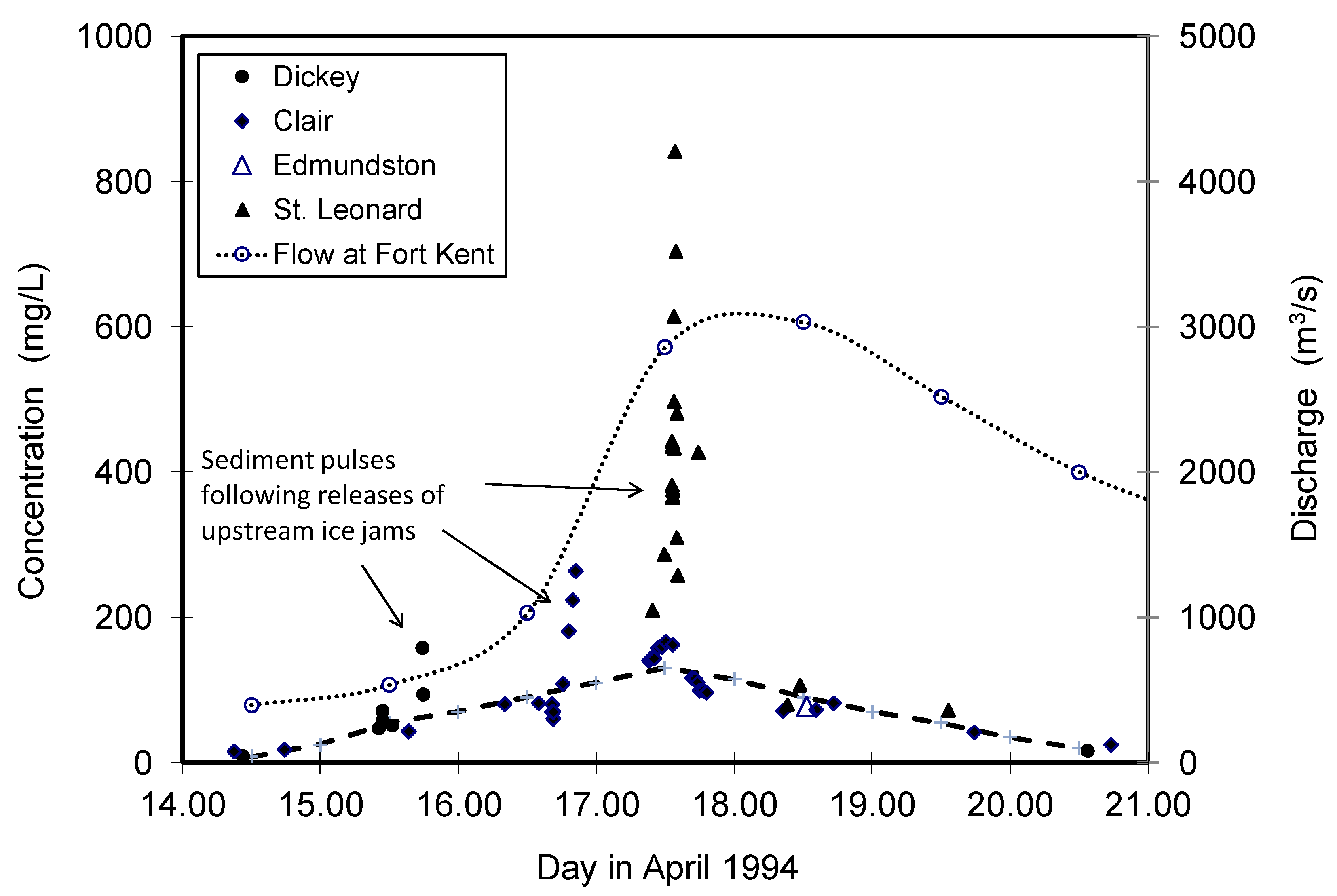
Comprehensive datasets on the height and duration of suspended-sediment pulses occurring during five breakup events (1993–1997) on the upper Saint John River (Maine (USA) and New Brunswick (Canada)) are presented in [53]. Figure 9 combines sedigraphs of the 1994 breakup event at four bridge sites along the river, Dickey and St. Leonard being the farthest upstream and downstream, respectively (approximate river distances between consecutive locations: 58 km Dickey to Clair, 34 km Clair to Edmundston, and 42 km Edmundston to St. Leonard). The small pulse at Clair on 16 April was preceded by the release of an ice jam located ~39 km upstream. The release occurred at ~1140 h and produced a 0.3 m wave height at the Ft. Kent gauge, which is located 1.3 km downstream of the Clair bridge. The ice from the released jam was arrested again at ~21 km upstream of Clair. The new jam may have advanced closer to Clair after that time and released very late on the 16th or very early on the 17th, producing a 3-m jave at the Fort Kent gauge in the morning of the 17th. The accompanying ice run was starting to thin out at Clair by 0630 h on the 17th and advanced to well beyond St. Leonard, where the largest sediment pulse was recorded on 17 April.

A temporal association exists between sediment pulses and the ice runs that accompany various javes (Figure 10). The pulses are caused by the amplified erosive capacity of the flow during the passage of javes, while as many as three pulses per site have been observed during a breakup event. At a given location, the sediment pulse begins after and ends before the jave does. Depending on the intensity of the ice run that ensues upon ice-jam release, the peak of the pulse may coincide with the peak of the jave (moderate runs) or occur before it (heavy runs). It has been hypothesized that the latter outcome results from near-shore grounding of ice rubble, which shields the river banks from further erosion.

Javes produce much higher concentrations than would be expected from the gradual river response to runoff, ranging from 4.2 to 6.5 times the runoff-generated peaks in the Saint John River and attaining values of ~1000 mg/L or 1 g/L [53]. For the Athabasca River above Fort McMurray, known for highly dynamic breakups, it is estimated that jave-induced SSCs could exceed ~10 g/L [19].

The occurrence of sediment pulses during javes can be explained by increased sediment supply and flow velocity/shear stress upon release of an ice jam. Water levels upstream of ice jams rise, exposing more of the sources of sediment, such as river banks and floodplains, to flowing water. When the jams release, upstream water levels drop quickly, and water re-entering the channel potentially carries with it considerable sediment. Downstream of the former ice-jam location, water levels rise as the jave passes, exposing still-dry bank zones; at the same time, transient but very high flow velocities and shear stresses cause bed and bank erosion. Though javes are typically very brief relative to the duration of the breakup event, they can deliver significant sediment loads, owing to the amplified SSCs and concomitant flows [19,53].

Peak sediment concentrations and net loads delivered by breakup pulses depend on a variety of factors related to jave intensity and sediment availability. The data for the Saint John River at Clair as reported in [53] reveal that pre-pulse and peak pulse SSCs increase with “carrier” discharge, i.e., the runoff-generated discharge in the river, which prevails before or after jave events. However, the amount of scatter associated with peak values suggests that additional factors, such as jam location and channel morphology, also need to be taken into account. We are not aware of any bed load measurements performed during the passage of javes in rivers, but bed shear magnitudes inferred from RLAM applications suggest that bed mobilization and transport can be intense.

Initial quantitative understanding of bed load and suspended bed material transport could be developed by applying existing modelling capability [49,50] and by adaptation of other dynamic river ice models (e.g., River 1d; [65]) to include sediment transport/deposition equations. However, no known river ice model has bank erosion prediction capability.

6. Environmental Implications

6.1. Geomorphic Considerations

The presence of a floating ice cover modifies the magnitude and distribution of flow velocities and thus the boundary and internal shear stresses that affect transport of bed and suspended sediment. Significant scour can occur especially at the toe of an ice jam, where the downward protrusion of ice deflects flow towards the bed and increases velocity through a restricted flow area under the jammed ice. In rivers and streams with mobile bed material, channel geometry and the bed regime can change corresponding to changes in erosive force and sedimentation.

Sediment moving in a river channel can be classified as bedload, suspended load, and mixed load [66]. In suspended-load-dominated systems (suspended sediment 85–100% of total sediment load), floods deposit finer, more cohesive sediments on the floodplain and stream banks, and the channel becomes narrow and deeper and tends to meander. Streambed erosion predominates over channel widening [66]. Bedload-dominated channels (bedload sediment 35–70% of total sediment load) display stream deposition as gravel bars and islands in a relatively wide, steep channel. Erosion occurs mainly from channel widening [66]. Mixed-load dominated channels experience both modes of sedimentation. The characteristics of suspended load-, mixed load- and bedload-dominated channels were expanded upon in [67]. The type of system (bedload, suspended load, or mixed load) can be delineated based on the Shields shear stress and the Reynolds number. The observed properties of the stream channel (channel pattern) can be used to infer sediment transport and depositional processes [68]. A river’s response to changes in streamflow and sediment transport can be evaluated using Lane’s relationship, where the product of flow discharge and energy slope is proportional to the product of sediment transport and median transport rate [69].

Sediment supply and deposition, including during the winter and ice-breakup period, should be considered when determining the functioning and operational life of a dam and reservoir. Dam construction alters the natural equilibrium between sediment dynamics and morphology along a river, including downstream impacts on river morphology and ecology due to a disruption in sediment continuity [70]. Some degree of sediment inflow and deposition occurs in all reservoirs formed by dams [70,71]. Sedimentation can reduce the longevity, usefulness, and sustainable operations of both storage reservoirs and run-of-the-river projects [72,73]. Generally, coarser sediments deposit in the upper ends of reservoirs, while finer suspended sediments may flow though the outlet works or deposit in the reservoir nearer the dam [70,71]. Factors affecting sediment deposition in reservoirs include the supply of sediment from upstream and the shoreline of the reservoir, sediment characteristics, reservoir dimensions and shape (that affects the flow-velocity distribution), and the outflow or sluicing of sediment at a dam’s outlet works. Trap efficiency, the ratio of the quantity of deposited sediment to the total sediment inflow, is affected by the sediment particle fall velocity (dependent upon particle size and shape and upon water viscosity and chemistry) and the rate of flow through the reservoir (subject to reservoir storage and rate of outflow) [71].

Flow regulation can alter channel morphology of ice-affected rivers. Widespread geomorphological changes, including the loss of sinuosity and the widening of the active unvegetated channel, have been observed along the Aishihik River, Yukon, and attributed mainly to the effect of regulation on river-ice processes [74]. In addition to other factors, downstream transport and deposition characteristics of the river may be significantly modified because ice breakup regimes can change considerably under regulation [75]. Such changes should be carefully considered in planning new projects or in assessing environmental impacts of existing projects. Because ice breakup and jamming processes are influenced by antecedent freezeup and winter conditions, in addition to the flow hydrograph, the entire regulated ice regime would have to be studied.

6.2. Water Quality Considerations

Trace element and organic contaminant concentrations will vary in bed sediment depending on the physical and chemical characteristics of the sediment and the concentrations of various contaminants. Sorption capacity of bed materials generally increases with decreasing particle size. Therefore, clay would be expected to have a greater capacity for surface coatings of carbonates, organic matter; and hydrous oxides of iron (Fe), aluminium (Al), and manganese (Mn) than sand [76]. Finer materials are deposited to bed sediments in fluvial systems during the under-ice period, leading to an accompanying increase in sediment TOC content and in the concentrations of a variety of trace elements [76].

Ice jams are important agents affecting sediment metal concentrations in rivers [77]. Following a large ice jam and associated flooding in February 1996 on the Blackfoot and Clark Fork Rivers of western Montana, large amounts of fine-grained sediment were mobilized such that metal concentrations in sediment downstream from a reservoir containing large amounts of contaminated sediment were enriched in metals, while open reaches above the reservoir were diluted [77].

Many water-quality contaminants travel as sorbed constituents on suspended-sediment particles, and thus water quality can be related to the suspended-sediment transport. To examine the concentrations of trace metals, 13 pairs of simultaneous water samples were obtained by dip sampling during the breakup event of 1997 at three bridge sites (Clair, Edmundston and St. Leonard) across the Saint John River, New Brunswick [52]. Environment Canada’s National Laboratory for Environmental Testing (NLET) in Burlington, Ontario analysed different samples from each set for dissolved and total concentrations of 17 metals: aluminium (Al), barium (Ba), beryllium (Be), cadmium (Cd), chromium (Cr), cobalt (Co), copper (Cu), iron (Fe), lead (Pb), lithium (Li), manganese (Mn), molybdenum (Mo), nickel (Ni), silver (Ag), strontium (Sr), vanadium (V), and zinc (Zn). For the study stretch of the Saint John River, the highest metal concentrations often occur during the breakup period when suspended-sediment concentrations are highest [52,78,79]. Measured breakup concentrations of aluminium, iron, and copper exceeded measured open-water values potentially by an order of magnitude; however, the highest open-water values of zinc (to 0.12 mg/L) exceeded breakup values [52].

A strong metal association with suspended sediment is evinced as total metal concentration tends to increase with suspended-sediment concentration [52]. For the data obtained on the study stretch of the Saint John River, total metal concentration (unfiltered sample), C_T, could be determined from a linear relationship:

$$C_T=s C_s+ C_w$$

(7)

in which s = particulate metal concentration expressed as mass of metal per unit mass of suspended sediment, C_s = suspended-sediment concentration, and C_w = dissolved metal concentration (filtered sample).

As C_W is usually a small part of C_T, the total metal content is largely governed by the value of the SSC. The particulate metal concentration, s, may be decreasing, increasing, or trendless with respect to discharge [80]. For the SJR data, an increasing value of s with increasing discharge was the general case for copper (Cu) and zinc (Zn), while a decreasing value of s with increasing discharge was found for several other metals (Al, Ba, Cd, Co, Cr, Fe, Li, Mn, Ni, Pb, Sr, and V). Despite the variability of s with discharge, it is still possible to use for practical purposes an appropriate value of s and an average value of C_W to estimate total metal concentration [52].

The surface area of sediment per unit mass and the sorption distribution coefficient are two important factors affecting the variability of the particulate trace metal concentration. The surface area of the sediment particles per unit mass, A_m, reflects the area for sorption and relates to relevant chemical processes [81]. Assuming thin platelets and using an average median size (D₅₀) of about 11 μm for the primary sediment particles, the estimated surface area of the sediment particles per unit mass, A_m, at the metal-sampling sites on the Saint John River is ≈7 m²/g [52]. The sorption distribution coefficient (particulate metal concentration (mass of metal per unit mass of suspended sediment) divided by the dissolved metal concentration) was reported as 5.2, 4.1, 5.0, 4.2, 5.4, 5.6, 2.7, 5.1, and 4.4 for AL, Ba, Cr, Cu, Fe, Mn, Ni, Pb, Sr, V, and Zn, respectively [52]. These values are in approximate agreement with values obtained elsewhere, as compiled in [82].

River ice can also be a depository for various substances, including toxic elements, as evinced by studies of ice in the Amur River, Russia [83]. The deposition of these substances is the result of ice interacting with flowing water and the river bed and banks as well as of the settling of atmospheric particles (including aerosols and suspended particulates) on the ice surface. The freezeup period provides environmental conditions for the accumulation of these substances into the ice cover and for transport, sedimentation, migration, and transformation of biogenic elements, suspended particulates, and dissolved organic matter [83]. Processes occurring during ice-cover growth also may change the migration ability of many heavy metals, thereby creating conditions for buildup of more toxic compounds [83]. During the melting and breakup of ice in springtime, these pollutants can enter the water and are thus unloaded into aquatic ecosystems [83].

The long-term retention and accumulation of metals in riverine aquatic environments can be detrimental to biota and ecosystem processes regardless of hydroclimatic setting and metal source (point or non-point, natural or anthropogenic). Metals on sediment that deposits on the channel bed can become dissolved into the water column over time and possibly bioaccumulate in living organisms. The amount of deposited substance can be effectively quantified by considering load rather than concentration, with a more accurate annual or seasonal estimate of substance loading obtained if sediment processes during breakup are not ignored.

6.3. Ecological Considerations

Scrimgeour et al. [84] reviews the effects of ice-cover breakup on aquatic systems, and Prowse [85,86] describes how river-ice phenomena and processes affect hydrologic, geomorphic, and chemical characteristics of a river and the associated biological consequences. Yet, complete understanding of how winter conditions affect aquatic ecosystems is lacking [87]. Linking changes in ice cover with river ecology is difficult because information about ice in small rivers and about ecology in the large rivers is lacking [88]. In this subsection, consideration is given to the effects of sediment transport and higher SSCs on aquatic species, aquatic habitat, and riverbank species, including vegetation.

River-ice processes change conditions for aquatic life by preventing reaeration (and thus reducing dissolved oxygen levels) in ice-covered rivers; by changing physical and chemical parameters in the under-ice flow, such as light intensity, temperature, stream velocity, and contaminant mixing; by creating a surface barrier that alters the prey–predator relationship, and by changing the amount of sediment transport and deposition. Changes in geomorphology, temperature regimes, and hydraulic connectivity along a river that affect biological and chemical processes can vary from headwaters to river mouth, with these changes likely greater in larger river systems [88]. A direct, physical effect upon biota can be more likely in small to medium streams of shallow depth than larger deeper rivers due to the greater possibility in small to medium streams of ice damming (freezing to the channel bed), anchor-ice formation, and ice scouring of the channel bed [88]; the latter two processes potentially add sediment to the river flow.

Aquatic biota respond to both the concentration of suspended sediments and duration of exposure, much as they do for other environmental contaminants; regression analysis indicates that SSC alone is a relatively poor indicator of effects on aquatic life [89]. The severity of the effects of suspended sediment also depends upon taxonomic group, life stage, and life history of the affected biota; the particle size, angularity, and toxicity of the suspended sediment; and duration of exposure to SSCs above normal background levels. In most cases, elevated suspended sediments cause sublethal effects, as some species can tolerate very high levels of suspended solids within a short period of time. However, harmful effects in ultrasensitive species and in species during certain life stages may occur once a threshold concentration of suspended sediment is abruptly exceeded [90]. Elevated suspended-sediment concentrations can lead to stress that increases vulnerability to other environmental stressors, such as water pollutants.

Considerable evidence exists to indicate that changes in the abundance and composition of invertebrate communities are associated with increases in suspended solids and turbidity [91,92]. Sediment can also directly affect invertebrates by clogging the filter mechanisms of bottom feeders or harming by abrasion the gills impairing respiration [89]. Excess deposition of sediment in coarse substrates will cover and inundate the gravels, thereby eliminating the habitat where many invertebrates live [91,92,93,94]. Ice regimes in temperate rivers can also affect organic-matter dynamics and feeding ecology of aquatic insects [95].

Elevated levels of suspended sediments can impact fish by physically damaging tissues and organs. Fine sediment can easily damage fish gills, with angular sediment particles usually more damaging to gills than larger or rounded particles. The scouring and abrasive action of suspended particles can damage gill tissues or clog gills [96]. If fish gills are irritated over sufficient time, mucus that forms to protect the gill can impede respiration [90,96,97,98]. Physical damage and clogging of the gills can increase fish susceptibility to infection and disease, reduce growth rates, and even result in fish mortality if high SSCs persist over a prolonged period [90,96]. Although it depends upon the species and life stage, moderate and severe gill damage may occur when SSCs exceed 100 mg/L and 500 mg/L, respectively [96]. Sediment mineralogy and the presence of innate or adsorbed toxicants may affect fish at the tissue and cellular level [90]. Kemp et al. [92] review the impacts of fine sediment on fish physiology and performance, including stream and sediment characteristics that affect the effect of fine sediment on fish (Table 1 of [92]) and the temporal responses of fish to fine sediment (Table 2 of [92]). Table 1 of [99] identifies the mortality effects of suspended-sediment levels by fish species. Affandi and Ishak [98] reviews the effects of turbidity, suspended sediment, and metal pollution on fish populations and riverine ecosystem, noting that the health of fish and their abundance also represent the health of their corresponding water bodies.

Elevated levels of suspended sediments can also impact fish by increasing physiological stress. The physiological stress caused by exposure to elevated SSCs over time can make fish more susceptible to disease [96]. The physiological effects of suspended sediments on fish are influenced by water temperatures, as dissolved oxygen is higher, and fish exhibit reduced activity (and metabolic rate) at cooler temperatures [91].

Suspended sediments also indirectly affect fish by changing water clarity (increased turbidity), which can alter fish movement or migration patterns, feeding success, and habitat quality [96]. Suspended solids have significant effects on community dynamics when they interfere with light transmission because of turbidity [93]. These factors also create stress levels that can trigger, over time, damaging physiological effects. Several researchers have investigated the effects of SSCs on fish avoidance of areas of high SSC by moving to areas of lower SSC. Knack and Shen [100] reviews existing studies on fish behaviour during the winter in ice-affected climates. Fish, particularly salmon, are sight feeders [91]. Turbidity decreases the ability of fish to find food and this, over time, may affect their health and rate of growth. Turbid water results in a stress response in salmonids.

Aggregates of fine sediment containing organic material is a primary source of food and energy for river ecosystems. The ability of taxa to adapt to variability in suspended loads and turbidity under natural conditions characterize natural ecosystems, creating opportunities for some species and affecting the structure of biological communities [92]. Short-term physiological and behavioural effects of fish affect the survival of a local fish population to high suspended-sediment loads; however, such exposure events may also have intergenerational ramifications that affect fish condition, survival, populations, and communities [99]. Recovery of a fish population from a sediment pulse depends on the magnitude and period of the sediment perturbation and sediment composition [92].

International guidelines for suspended sediment vary. The Canadian Water Quality Guidelines for the Protection of Aquatic Life provide target limits for total particulate matter in freshwater, estuarine, and marine environments with respect to suspended sediments, turbidity, deposited bedload sediments, and streambed substrate [101]. In clear stream systems, small, induced exceedances in suspended-sediment concentration above a 25 mg/L change from background levels for short-term exposure (e.g., 24 h) can cause behavioural and low sublethal effects on fish, all of which are reversible (CCME 2002). During high flows, an increase of 25 mg/L when sediment levels are between 25 mg/and 250 mg/L or by 10% or more when sediment levels exceed 250 mg/L is considered detrimental to aquatic life. Information in technical literature as cited in this paper shows that such increases can occur during breakup. For longer term exposure (e.g., 30 d or more), an increase in average suspended-sediment concentrations by more than 5 mg/L over background levels is identified as of concern [101]. In Europe, suspended-sediment concentrations should not exceed 25 mg/L for salmonid and cyprinid habitats [96].

Exposure to certain chemical substances represents a potentially significant hazard to the health of the organisms. Sediment quality guidelines contain information regarding the relationships between the chemical concentrations associated with sediment and adverse biological effects resulting from exposure to these chemicals [101].

Habitat requirements shift with ontogenetic development [92]. Fish eggs are an especially vulnerable life stage due to their immobility and the requirements for specific hydraulic and substrate conditions [102]. Deposition and the infilling of gravel bed material by finer sediment can reduce survival of fish eggs by reducing clean water flow and oxygen from reaching the eggs and by preventing newly hatched fish from migrating through the gravel and emerging as fry [91]. Generally, stable discharges and low sediment discharge are more favourable to the survival of salmonids in the early stages of life than sudden changes in flow and sediment discharge. Small amounts of fine sediment in salmonid redds can diminish survivability and emergence of fish from eggs. The intrusion of fine sediments into a gravel streambed depends upon the initial concentration of suspended sediment; the roughness and particle size distribution of the bed material; and flow characteristics, such as discharge, water depth, velocity, and shear stress [103]. Kemp et al. [92] discussed the spawning traits and incubation periods of several benthic spawning freshwater fish, detailing the spawning habitat, egg characteristics, incubation period, and potential impacts of fine sediments (Table 3 of [92]). As is the case for eggs, larval and juvenile stages are more susceptible to the effect of fine sediment than adults, which have a greater propensity to move and avoid adverse conditions [104].

Hydro-morphological conditions in rivers can affect fish habitat, which can have important effects on fish mortality during the winter months. Knack and Shen [100] presents proposed fish-habitat preferences for salmonids in winter. Habitat suitability curves were developed for use with a two-dimensional, hydro-thermal-ice-sediment river dynamics model, RICE2D. They simulated river conditions with the RICE2D model coupled with an IFIM and PHABSIM-type fish-habitat-suitability model, which includes thermal-ice as well as sediment and bed-change conditions in rivers to allow a detailed habitat suitability evaluation. The impact of the dam removal on the St. Regis River, Hogansburg, NY, USA, on fish habitat was evaluated, showing an improvement in fish habitat for both open-water and ice-affected conditions in the restored reach. Model results show that there would be no significant overall loss of wintertime fish habitat from the removal of the dam despite increased frazil ice production [100]. The model is a useful assessment tool for exploring fish habitat during the winter ice periods and for evaluating fish-habitat restoration for all seasons.

In addition to aquatic fauna, the geomorphologic processes associated with ice breakup (see Section 3.1) also affect vegetation. The amount of ice-related stress or disturbance that a plant species can tolerate and its capability to recover after an ice-related disturbance depends upon its physiology and the nature of the disturbance [105]. Tree scars, a phenomenon that occurs when ice shoves against trees along the riverbank, and trim lines, the lower limit of a vegetative community longitudinally along a river, can provide information on the elevation of past ice-jam events (e.g., [105]). In some cases, ice scour and the transport of sediment and organic matter can contribute to the dissemination and available habitat of plant species. For example, the population of Furbish’s lousewort (Pedicularis furbishiae), an endangered herbaceous perennial plant that occurs on the intermittently flooded 140-km long stretch of Saint John River in northern Maine and northwestern New Brunswick, is dependent on the presence of appropriate host plants, moist soils, and pollinators and on habitat created by periodic ice scour, providing the occurrence of ice-related scour is not too frequent or rare [106].

In addition, ice-jam-related flooding and replenishment with water, sediment, and nutrients can be critical to the ecosystem vitality of northern river-delta environments, such as the Mackenzie River Delta and the Peace-Athabasca Delta in northern Canada. This is particularly concerning if perched ponds and lakes are too high to be recharged by the open-water flow system [107,108].

7. Concluding Remarks

Compared to midwinter periods under a stable ice cover, forces acting to dislodge material from a river bank during the pre-breakup and breakup periods not only increase, but rising water levels may expose a greater portion of the bank to these forces. This results in increased sediment transport, which can have potential effects on channel morphology, reservoir operations, water quality, aquatic life and habitat, and riparian ecology.

Under a changing and progressively warmer climate, an increase in the number of midwinter breakups and the magnitude of breakup flows may result in a considerable increase in future sediment concentrations and loads during the pre-breakup and breakup periods. Projections of regional climate change need to be inputted in hydrologic and hydrodynamic models to determine the physical changes in surface runoff and streamflow that may alter sediment supply, transport, and deposition in rivers with seasonal ice covers.

Many northern rivers exhibit low background suspended-sediment concentrations prior to breakup, but suspended-sediment concentrations increase by at least an order of magnitude prior to and during breakup. Suspended-sediment concentrations during javes can be even greater and far exceed those of open-water events. Therefore, to estimate the total annual load in a river, it is necessary to consider the amount of suspended sediment delivered during the breakup period. An increase in suspended-sediment concentrations during breakup is of interest due to their effect on aquatic ecosystems in terms of both species’ life cycle and habitat and on water quality due to the sorption of particulate contaminants onto sediment particles.

Scientific studies have shown that suspended-sediment loads during the breakup period may be a major portion of the annual sediment load on some rivers. Yet, existing sediment monitoring programs normally do not capture the increased suspended-sediment concentrations and loads that occur briefly during the ice breakup event. A more accurate estimate of sediment loads on a river may be obtainable from more frequent measurements of suspended sediment during the breakup period, but large-scale collection of sediment data during breakup is likely to be difficult and costly.

As revealed in scientific literature, high sediment concentrations, especially when associated with metal contaminants, can have detrimental effects on water quality and ecosystem robustness. Total metal concentration tends to increase with suspended-sediment concentration. Along a stretch of the Saint John River, high metal concentrations were found generally to occur during the breakup period when suspended-sediment concentrations are high.

Further research is needed to relate sediment concentrations and loads, including those generated by sediment pulses, to breakup conditions and underlying hydro-climatic and geomorphological variables and hence develop predictive mathematical models. Affordable instrumentation and data-interpretation software could also be developed and applied to obtain adequate field datasets for model calibration.

References

- Burrell, B.C.; Beltaos, S. Effects and Implications of River Ice Breakup on Suspended-Sediment Concentrations: A synthesis. In Proceedings of the CGU HS Committee on River Ice Processes and the Environment 20th Workshop on the Hydraulics of Ice-Covered Rivers, Ottawa, ON, Canada, 14–16 May 2019; Available online: http://www.cripe.ca/docs/proceedings/20/Burrell-Beltaos-2019.pdf (accessed on 10 September 2021).
- Beltaos, S. (Ed.) River Ice Breakup; Water Resources Publications, LLC: Highlands Ranch, CO, USA, 2008; 462p. [Google Scholar]
- Beltaos, S. Hydrodynamic characteristics and effects of river waves caused by ice jam releases. Cold Reg. Sci. Technol. 2013, 85, 42–55. [Google Scholar] [CrossRef]
- Turcotte, B.; Burrell, B.C.; Beltaos, S. The Impact of Climate Change on Breakup Ice Jams in Canada: State of knowledge and research approaches. In Proceedings of the 20th Workshop on the Hydraulics of Ice Covered Rivers, Ottawa, ON, Canada, 14–16 May 2019; Available online: http://www.cripe.ca/docs/proceedings/20/Turcotte-et-al-2019.pdf (accessed on 15 September 2021).
- Beltaos, S.; Prowse, T. River-ice hydrology in a shrinking cryosphere. Hydrol. Process. 2009, 23, 122–144. [Google Scholar] [CrossRef]
- Kämäri, M.; Alho, P.; Veijalainen, N.; Aaltonen, J.; Huokuna, M.; Lotsari, E. River ice cover influence on sediment transportation at present and under projected hydroclimatic conditions. Hydrol. Process. 2015, 29, 4738–4755. [Google Scholar] [CrossRef]
- Chassiot, L.; Lajeunesse, P.; Bernier, J.-F. Riverbank erosion in cold environments: Review and outlook. Earth-Sci. Rev. 2020, 207, 103231. [Google Scholar] [CrossRef]
- Gatto, L.W. Riverbank Conditions and Erosion during Winter. In Proceedings of the Workshop on Environmental Aspects of River Ice, Saskatoon, SK, Canada, 18–20 August 1993; Prowse, T.D., Ed.; NHRI Symposium Series No. 12. National Hydrology Research Institute: Saskatoon, SK, Canada, 1993; pp. 43–56. [Google Scholar]
- Vandermause, R.A. The Role of Dynamic Ice-Breakup on Bank Erosion and Lateral Migration of the Middle Susitna River, Alaska. Master’s Thesis, Department of Civil and Environmental Engineering, Colorado State University, Fort Collins, CO, USA, 2018; 334p. Available online: https://mountainscholar.org/handle/10217/191335?show=full (accessed on 10 September 2021).
- Vandermause, R.; Harvey, M.; Zevenbergen, L.; Ettema, R. River-ice effects on bank erosion along the middle segment of the Susitna river, Alaska. Cold Reg. Sci. Technol. 2021, 185, 103239. [Google Scholar] [CrossRef]
- Vandermause, R.; Ettema, R. Aerial Monitoring of Vegetation to Identify Ice-related Bank Erosion Along the Middle Reach of the Susitna River, Alaska. In Proceedings of the CGU HS Committee on River Ice Processes and the Environment 19th Workshop on the Hydraulics of Ice Covered Rivers, Whitehorse, YK, Canada, 9–12, July 2017. [Google Scholar]
- Ettema, R.; Kempema, E.W. Chapter 9: Ice effects on sediment transport. In River Ice Formation; Beltaos, S., Ed.; Committee on River Ice Processes and the Environment, Canadian Geophysical Union Hydrology Section: Edmonton, AB, Canada, 2013; pp. 297–338. [Google Scholar]
- Turcotte, B.; Morse, B.; Bergeron, N.E.; Roy, A.G. Sediment transport in ice-affected rivers. J. Hydrol. 2011, 409, 561–577. [Google Scholar] [CrossRef]
- Ettema, R. Review of Alluvial-Channel responses to River Ice. J. Cold Reg. Eng. 2002, 16, 191–217. [Google Scholar] [CrossRef]
- Gatto, L.W. Soil Freeze-Thaw Effects on Bank Erodibility and Stability; CRREL Special Report 95-24; Cold Regions Research and Engineering Laboratory: Hanover, NH, USA, 1995; 24p. [Google Scholar]
- Chow, V.T. Open Channel Hydraulics; McGraw-Hill Book Company: New York, NY, USA, 1959. [Google Scholar]
- Yalin, M.S. Mechanics of Sediment Transport; Pergamon Press: Oxford, UK, 1977; 360p, ISBN 978-0080211626. [Google Scholar]
- Beltaos, S.; Carter, T.; Rowsell, R.; DePalma, S.G.S. Erosion potential of dynamic ice breakup in Lower Athabasca River. Part I: Field measurements and initial quantification. Cold Reg. Sci. Technol. 2018, 149, 16–28. [Google Scholar] [CrossRef]
- Beltaos, S. Erosion potential of dynamic ice breakup in Lower Athabasca River. Part II: Field data analysis and interpretation. Cold Reg. Sci. Technol. 2018, 148, 77–87. [Google Scholar] [CrossRef]
- Annandale, G.W. Erodibility. J. Hydraul. Res. 1995, 33, 471–494. [Google Scholar] [CrossRef]
- Turcotte, B.; Morse, B. The Winter Environmental Continuum of Two Watersheds. Water 2017, 9, 337. [Google Scholar] [CrossRef]
- Hicklin, E.J. Chapter 4: Sediment transport. In Rivers. Course Notes for an Undergraduate Course in Fluvial Geomorphology; Department of Geography, Simon Fraser University: Burnaby, BC, Canada, 2009; Available online: http://www.sfu.ca/~hickin/RIVERS/Rivers4%28Sediment%20transport%29.pdf (accessed on 16 March 2021).
- Knighton, D. Fluvial Forms and Processes: A New Perspective; Arnold: London, UK, 1998; 383p. [Google Scholar]
- Robert, A. River Processes: An Introduction to Fluvial Dynamics; Arnold: London, UK, 2003; ISBN 978-0340763391. [Google Scholar]
- Van Rijn, L.C. Sediment Transport, Part II: Suspended Load Transport. J. Hydraul. Eng. 1984, 110, 1613–1641. [Google Scholar] [CrossRef]
- Tsujimoto, T. Diffusion coefficient of suspended sediment and kinematic eddy viscosity of flow containing suspended load. In River Flow 2010; Dittrich, A., Koll, K., Aberle, J., Geisenhainer, P., Eds.; Bundesanstalt für Wasserbau S.: Karlsruhe, Germany, 2010; pp. 801–806. [Google Scholar]
- Syvitski, J.; Cohen, S.; Miara, A.; Best, J. River temperature and the thermal-dynamic transport of sediment. Glob. Planet. Chang. 2019, 178, 168–183. [Google Scholar] [CrossRef]
- Fondriest Environmental, Inc. Turbidity, Total Suspended Solids and Water Clarity. Fundamentals of Environmental Measurements. 13 June 2014. Available online: https://www.fondriest.com/environmental-measurements/parameters/water-quality/turbidity-total-suspended-solids-water-clarity/ (accessed on 10 September 2021).
- Kempema, E.W.; Ettema, R.; Bunte, K. Anchor-ice rafting, an important mechanism for bed-sediment transport in cold-regions rivers. In River Flow 2020; Taylor and Francis: Oxfordshire, UK, August 2020. [Google Scholar] [CrossRef]
- Kalke, H.; McFarlane, H.; Schneck, C.; Loewen, M. The transport of sediments by released anchor ice. Cold Reg. Sci. Technol. 2017, 143, 70–80. [Google Scholar] [CrossRef]
- Maclean, B.; Bampfylde, C.; Lepine, M.; Tssessaze, L. Towards a Rights-Based Ice Monitoring Trigger. In Proceedings of the 21st Workshop on the Hydraulics of Ice Covered Rivers, Saskatoon, SK, Canada, 29 August–1 September 2021. [Google Scholar]
- Lawson, D.E.; Chacho, E.F., Jr.; Brockett, B.E.; Wuebben, J.L.; Collins, C.M.; Arcone, S.A.; Delaney, A.J. Morphology, Hydraulics and Sediment Transport of an Ice-Covered River: Field Techniques and Initial Data; CRREL Report 86-11; U.S. Army Cold Regions Research and Engineering Laboratory: Hanover, NH, USA, 1986; 49p.
- Prowse, T.D. Suspended sediment concentration during breakup. Can. J. Civ. Eng. 1993, 20, 872–875. [Google Scholar] [CrossRef]
- Beltaos, S.; Burrell, B.C. Transport of suspended sediment during the breakup of the ice cover, Saint John River, Canada. Cold Reg. Sci. Technol. 2016, 129, 1–13. [Google Scholar] [CrossRef]
- Ferrick, M.G.; Weyrick, P.B. On the Sediment Carrying Capacity of Rivers during Ice Breakup. In Proceedings of the Workshop on Environmental Aspects of River Ice, Saskatoon, SK, Canada, 18–20 August 1993; Prowse, T.D., Ed.; NHRI Symposium Series No. 12. National Hydrology Research Institute: Saskatoon, SK, Canada, 1993; pp. 161–175. [Google Scholar]
- Beltaos, S. Chapter 7. Freezeup jamming and formation of ice cover. In River Ice Formation; Beltaos, S., Ed.; CGU-HS Committee on River Ice Processes and the Environment (CRIPE): Edmonton, AB, Canada, 2013; pp. 181–255. [Google Scholar]
- Gerard, R. Preliminary observations of spring ice jams in Alberta. In Proceedings of the International Association for Hydraulic Research Ice Symposium, Hanover, NH, USA, 18–21 August 1975; pp. 261–277. [Google Scholar]
- Andres, D.D.; Rickert, H.A. Observations of the 1985 Breakup in the Athabasca River Basin Upstream of Fort McMurray, Alberta; Report No. SWE 85-10; Alberta Research Council: Edmonton, AB, Canada, 1985; 74p. [Google Scholar]
- Jasek, M.; Beltaos, S. Chapter 8. Ice-jam release: Javes, ice runs and breaking fronts. In River Ice Breakup; Water Resources Publications: Highlands Ranch, CO, USA, 2008. [Google Scholar]
- She, Y.; Hicks, F. Modelling ice jam release waves with consideration for ice effects. Cold Reg. Sci. Technol. 2006, 45, 137–147. [Google Scholar] [CrossRef]
- Kowalczyk Hutchison, T.; Hicks, F.E. Observations of ice jam release waves on the Athabasca River near Fort McMurray, Alberta. Can. J. Civ. Eng. 2007, 34, 473–484. [Google Scholar] [CrossRef]
- She, Y.; Andrishak, R.; Hicks, F.; Morse, B.; Stander, E.; Krath, C.; Keller, D.; Abarca, N.; Nolin, S.; Nzokou Tanekou, F.; et al. Athabasca River ice jam formation and release events in 2006 and 2007. Cold Reg. Sci. Technol. 2009, 55, 249–261. [Google Scholar] [CrossRef]
- Nafziger, J.; She, Y.; Hicks, F. Celerities of waves and ice runs from ice jam releases. Cold Reg. Sci. Technol. 2016, 123, 71–80. [Google Scholar] [CrossRef]
- Beltaos, S.; Burrell, B.C. Field measurements of ice-jam-release surges. Can. J. Civ. Eng. 2005, 32, 699–711. [Google Scholar] [CrossRef]
- Henderson, F.M. Open Channel Flow; The Macmillan Company: New York, NY, USA, 1996; 544p, ISBN 978-0023535109. [Google Scholar]
- Beltaos, S.; Burrell, B.C. Determining ice-jam surge characteristics from measured wave forms. Can. J. Civ. Eng. 2005, 32, 687–698. [Google Scholar]
- Beltaos, S.; Rowsell, R.; Tang, P. Remote data collection on ice breakup dynamics: Saint John River case study. Cold Reg. Sci. Technol. 2011, 67, 135–145. [Google Scholar] [CrossRef]
- Knack, I.M.; Shen, H.T. Numerical Modeling of Ice Transport in Channels with River Restoration Structures. Can. J. Civ. Eng. 2017, 44, 813–819. [Google Scholar] [CrossRef]
- Knack, I.M.; Shen, H.T. A Numerical Model for Sediment Transport and Bed Change with River Ice. J. Hydraul. Res. 2018, 56, 844–856. [Google Scholar] [CrossRef]
- Manolidis, M.; Katopodes, N. Bed Scouring During the Release of an Ice Jam. J. Mar. Sci. Eng. 2014, 2, 370–385. [Google Scholar] [CrossRef] [Green Version]
- Knack, I.; Clarkson University, Potsdam, NY, USA. Personal communication, March 2021.
- Beltaos, S.; Burrell, B.C. Characteristics of suspended sediment and metal transport during ice breakup, Saint John River, Canada. Cold Reg. Sci. Technol. 2016, 123, 164–176. [Google Scholar] [CrossRef]
- Beltaos, S. Extreme sediment pulses during ice breakup, Saint John River, Canada. Cold Reg. Sci. Technol. 2016, 128, 38–46. [Google Scholar] [CrossRef]
- Lai, Y.G. Modeling Stream Bank Erosion: Practical Stream Results and Future Needs. Water 2017, 9, 950. [Google Scholar] [CrossRef] [Green Version]
- Milburn, D.; Prowse, T.D. Observations on Some Physical-Chemical Characteristics of River-Ice Breakup. J. Cold Reg. Eng. 2000, 14, 214–223. [Google Scholar] [CrossRef]
- Milburn, D.; Prowse, T.D. The effect of river-ice breakup on suspended sediment and select trace-element fluxes. Nord. Hydrol. 1996, 27, 69–84. [Google Scholar] [CrossRef]
- Sui, J.; Wang, D.; Karney, B.W. Suspended sediment concentration and deformation of riverbed in a frazil jammed reach. Can. J. Civ. Eng. 2000, 27, 1120–1129. [Google Scholar] [CrossRef]
- Toniolo, H.; Vas, D.; Prokein, P.; Kenmitz, R.; Lamb, E.; Brailey, D. Hydraulic characteristics and suspended sediment loads during spring breakup in several streams located on the National Petroleum Reserve in Alaska, USA. Nat. Resour. 2013, 4, 220–228. [Google Scholar] [CrossRef] [Green Version]
- Moore, S.A.; Zare, S.G.A.; Rennie, C.D.; Seidou, O.; Ahmari, H. Monitoring suspended sediment under ice using acoustic instruments: Presentation of measurements made under break-up. In Proceedings of the 17th Workshop on River Ice, Committee on River Processes and the Environment, Edmonton, AB, Canada, 21–24 July 2013. [Google Scholar]
- Shakibaeinia, A.; Dibike, Y.B.; Kashyap, S.; Prowse, T.D.; Droppo, I.G. A numerical framework for modelling sediment and chemical constituents transport in the Lower Athabasca River. J. Soils Sedim. 2017, 17, 1140–1159. [Google Scholar] [CrossRef]
- Skolasińska, K.; Nowak, B. What factors affect the suspended sediment concentrations in rivers? A study of the upper Warta River (Central Poland). River Res. Appl. 2018, 34, 112–123. [Google Scholar] [CrossRef]
- Kowalczyk, T.; Hicks, F. Observations of dynamic ice jam release on the Athabasca River at Fort McMurray, AB. In Proceedings of the 12th Workshop on the Hydraulics of Ice Covered Rivers, Edmonton, AB, Canada, 19–20 June 2003; CGU HS Committee on River Ice Processes and the Environment: Edmonton, AB, Canada, 2003; pp. 369–392. Available online: http://cripe.ca/docs/proceedings/12/Kowalczyk-Hicks-2003.pdf (accessed on 10 September 2021).
- Malcovish, C.D.; Andres, D.D.; Mostert, P. Observations of breakup on the Athabasca River near Fort McMurray, 1986 and 1987; Report SWE-88/12; Alberta Research Council: Edmonton, AB, Canada, 1988. [Google Scholar]
- Beltaos, S.; Kääb, A. Estimating river discharge during ice breakup from near-simultaneous satellite imagery. Cold Reg. Sci. Technol. 2014, 98, 35–46. [Google Scholar] [CrossRef] [Green Version]
- Blackburn, J.; She, Y. A comprehensive public-domain river ice process model and its application to a complex natural river. Cold Reg. Sci. Technol. 2019, 163, 44–58. [Google Scholar] [CrossRef]
- Schumm, S.A. A Tentative Classification of Alluvial River Channels; Geological Survey Circular 477; US Geological Survey, United States Department of the Interior: Washington, DC, USA, 1963.
- Church, M. Bed material transport and the morphology of alluvial river channels. Annu. Rev. Earth Planet. Sci. 2006, 34, 325–354. [Google Scholar] [CrossRef]
- Burge, L.; Guthrie, R.; Chaput-Desrochers, L. Hydrological Factors Affecting Spatial and Temporal Fate of Sediment in Association with Stream Crossings of the Mackenzie Gas Pipeline; Canadian Science Advisory Secretariat Research Document 2014/029; Fisheries and Oceans Canada: Ottawa, ON, USA, 2014; 35p. [Google Scholar]
- Lane, E.W. The importance of fluvial morphology in hydraulic engineering. Proc. Am. Soc. Civil Eng. 1955, 81, 1–17. [Google Scholar]
- Schleiss, A.J.; Franca, M.J.; Juez, C.; De Cesare, G. Reservoir sedimentation. J. Hydraul. Res. 2016, 54, 595–614. [Google Scholar] [CrossRef]
- Strand, R.I.; Pemberton, E.L. Reservoir Sedimentation Technical Guideline for Bureau of Reclamation; Engineering and Research Center, Bureau of Reclamation: Denver, CO, USA, 1982; 48p.
- Palmieri, A.; Shah, F.; Annandale, G.W.; Dinar, A. Reservoir Conservation: The RESCON Approach; World Bank: Washington, DC, 2003; Available online: http://documents1.worldbank.org/curated/pt/819541468138875126/pdf/349540v10Reservoir0conservation0RESCON.pdf (accessed on 25 February 2019).
- Annandale, G.W.; Morris, G.L.; Karki, P. Extending the Life of Reservoirs: Sustainable Sediment Management for Dams and Run-of-River Hydropower. Directions in Development; World Bank: Washington, DC, USA, 2016. [Google Scholar] [CrossRef]
- McParland, D.; McKillop, R.; Pearson, F. Fluvial geomorphological responses to river ice dynamics downstream of a hydroelectric facility, southwest Yukon. In Proceedings of the Committee on River Processes and the Environment 21st Workshop on Hydraulics of River Ice, Saskatoon, SK, Canada, 29 August–2 September 2021. [Google Scholar]
- Huokuna, M.; Morris, M.; Beltaos, S.; Burrell, B.C. Ice in reservoirs and regulated rivers. Int. J. River Basin Manag. 2020. [Google Scholar] [CrossRef]
- Doig, L.E.; Carr, M.K.; Meissner, A.G.N.; Jardine, T.D.; Jones, P.D.; Bharadwaj, L.; Lindenschmidt, K.-E. Open-water and under-ice seasonal variations in trace element content and physicochemical associations in fluvial bed sediment. Environ. Toxicol. Chem. 2017, 36, 2916–2924. [Google Scholar] [CrossRef]
- Moore, J.N.; Landrigan, E.M. Mobilization of metal-contaminated sediment by ice-jam floods. Environ. Geol. 1999, 37, 96–101. [Google Scholar] [CrossRef]
- Beltaos, S.; Burrell, B.C. Suspended sediment concentrations in the Saint John River during ice breakup. In Proceedings of the 2000 Annual Conference of the Canadian Society for Civil Engineering, London, ON, Canada, 7–10 June 2000; pp. 235–242. [Google Scholar]
- Beltaos, S.; Burrell, B.C.; Ismail, S. Ice and sedimentation processes in the Saint John River, Canada. In Proceedings of the IAHR International Symposium on Ice, Trondheim, Norway, 11–21 August 1994; Volume 1, pp. 11–21. [Google Scholar]
- Miller, J.R.; Orbock Miller, S.M. Contaminated Rivers; Springer: Dordrecht, The Netherlands, 2007; 418p. [Google Scholar]
- Horowitz, A.J. A Primer on Sediment-Trace Element Chemistry, 2nd ed.; Lewis Publishers, Inc.: Chelsea, MI, USA, 1991. [Google Scholar]
- Allison, J.D.; Allison, T.L. Partition Coefficients for Metals in Surface Water, Soil, and Waste; EPA/600/R-05/074; U.S. Environmental Protection Agency: Washington, DC, USA, 2005; 93p.
- Golubeva, E.M.; Kondratyeva, L.M.; Shtareva, A.V.; Krutikova, V.O. Features of toxic element distribution in the Amur River Ice. Earth’s Cryosphere 2020, XXIV, 3–13. [Google Scholar] [CrossRef]
- Scrimgeour, G.J.; Prowse, T.D.; Culp, J.M.; Chambers, P.A. Ecological effects of river ice break-up: A review and perspective. Freshw. Biol. 1994, 32, 261–275. [Google Scholar] [CrossRef]
- Prowse, T.D. River-ice ecology. I. Hydrologic, geomorphic, and water-quality aspects. J. Cold Reg. Eng. 2001, 15, 1–16. [Google Scholar] [CrossRef]
- Prowse, T.D. River-ice ecology. II. Biological aspects. J. Cold Reg. Eng. 2001, 15, 17–33. [Google Scholar] [CrossRef]
- Lindenschmidt, K.-E.; Baulch, H.M.; Cavaliere, E. River and Lake Ice Processes—Impacts of Freshwater Ice on Aquatic Ecosystems in a Changing Globe. Water 2018, 10, 1586. [Google Scholar] [CrossRef] [Green Version]
- Thellman, A.; Jankowski, K.J.; Hayden, B.; Yang, X.; Dolan, W.; Smits, A.P.; O’Sullivan, A.M. The ecology of river ice. J. Geophys. Res. Biogeosci. 2021, 126, e2021JG006275. [Google Scholar] [CrossRef]
- Newcombe, C.P.; Macdonald, D.D. Effects of Suspended Sediments on Aquatic Ecosystems. N. Am. J. Fish. Manag. 1991, 11, 72–82. [Google Scholar] [CrossRef]
- Newcombe, C.P.; Jensen, J.O.T. Channel Suspended Sediment and Fisheries: A Synthesis for Quantitative Assessment of Risk and Impact. N. Am. J. Fish. Manag. 1996, 16, 693–727. [Google Scholar] [CrossRef]
- Kerr, S.J. Silt, Turbidity and Suspended Sediments in the Aquatic Environment: An Annotated Bibliography and Literature Review; Southern Region Science & Technology Transfer Unit Technical Report TR-008; Ontario Ministry of Natural Resources: Toronto, ON, Canada, 1995; 277p. [Google Scholar]
- Kemp, P.; Sear, D.; Collins, A.; Naden, P.; Jones, I. The impacts of fine sediment on riverine fish. Hydrol. Process. 2011, 25, 1800–1821. [Google Scholar] [CrossRef]
- Sorensen, D.L.; McCarthy, M.M.; Middlebrooks, E.J.; Porcella, D.B. Suspended and Dissolved Solids Effects on Freshwater Biota: A Review; Corvallis Environmental Research Laboratory, Office of Research and Development, U.S. Environmental Protection Agency: Corvallis, OR, USA, 1977; 73p.
- Gammon, J.R. The Effect of Inorganic Sediment on Stream Biota; Water Pollution Control Research Series 18050 DWC 12/70; Environmental Protection Agency: Washington, DC, USA, 1970; 141p.
- Blackadar, R.J.; Baxter, C.V.; Davis, J.M.; Harris, H.E. Effects of river ice break-up on organic-matter dynamics and feeding ecology of aquatic insects. River Res Appl. 2020, 36, 480–491. [Google Scholar] [CrossRef]
- Cavanagh, J.-E.; Hogsden, K.L.; Harding, J.S. Effects of Suspended Sediment on Freshwater; Landcare Research: Lincoln, New Zealand, 2014; 24p. [Google Scholar]
- Berg, L. The effect of exposure to short-term pulses of suspended sediment on the behaviour of juvenile salmonids. In Proceedings of the Carnation Creek Workshop: A Ten-Year Review, Nanaimo, BC, Canada, 24–26 February 1982; Hartman, G.F., Ed.; Department of Fisheries and Oceans, Pacific Biological Station: Nanaimo, BC, Canada, 1982; pp. 177–196. [Google Scholar]
- Affandi, F.A.; Ishak, M.Y. Impacts of suspended sediment and metal pollution from mining activities on riverine fish population—A review. Environ. Sci. Pollut. Res. 2019, 26, 16939–16951. [Google Scholar] [CrossRef]
- Kjelland, M.E.; Woodley, C.M.; Swannack, T.M.; Smith, D.L. A review of the potential effects of suspended sediment on fishes: Potential dredging-related physiological, behavioral, and transgenerational implications. Environ. Syst. Decis. 2015, 35, 334–350. [Google Scholar] [CrossRef] [Green Version]
- Knack, I.M.; Shen, H.T. Modeling fish habitat condition in ice affected rivers. Cold Reg. Sci. Technol. 2020, 176, 103086. [Google Scholar] [CrossRef]
- CCME (Canadian Council of Ministers of the Environment). Canadian water quality guidelines for the protection of aquatic life: Total particulate matter. In Canadian Environmental Quality Guidelines, 1999; Canadian Council of Ministers of the Environment: Winnipeg, MB, Canada, 2002. [Google Scholar]
- Cunjak, R.A.; Prowse, T.D.; Parrish, D.L. Atlantic salmon (Salmo salar) in winter: “The season of parr discontent?”. Can. J. Fish. Aquat. Sci. 1998, 55 (Suppl. S1), 161–180. [Google Scholar] [CrossRef]
- Glasbergen, K.A. The Effect of Coarse Gravel on Cohesive Sediment Entrapment. Master’s Thesis, Dept. of Geography, University of Waterloo, Waterloo, ON, Canada, 2013; 105p. [Google Scholar]
- Wood, P.J.; Armitage, P.D. Sediment deposition in a small lowland stream–management implications. Reg. Rivers-Res. Manag. 1999, 15, 199–210. [Google Scholar] [CrossRef]
- Uunila, L.S. Effects of River Ice on Bank Morphology and Riparian Vegetation along Peace River, Clayhurst to Fort Vermilion. In Proceedings of the 9th Workshop on River Ice, Fredericton, NB, USA, 24–26 September 1997; pp. 315–334. [Google Scholar]
- U.S. Fish and Wildlife Service. Species Status Assessment for the Furbish’s Lousewort (Pedicularis furbishiae), Version 1.1; Ecological Services Maine Field Office: East Orland, ME, USA, 2018; 59p + 3 appendices.
- Marsh, P.; Hey, M. The flooding hydrology of Mackenzie delta lakes near Inuvik, N.W.T. Canada. Arctic 1989, 42, 41–49. [Google Scholar] [CrossRef] [Green Version]
- Prowse, T.D.; Lalonde, V. Open-Water and Ice-Jam Flooding of a Northern Delta. Hydrol. Res. 1996, 27, 85–100. [Google Scholar] [CrossRef]
Figure 1.
Schematic illustration of a fully developed ice jam. The equilibrium reach is usually much longer than indicated in the sketch but may be absent in short jams. Reproduced from [36]. Crown copyright, published by CGU-HS Committee on River Ice Processes and the Environment.
Figure 2.
Passage of a 2002 jave in a 15 km reach of the Athabasca River, captured by temporary water level gauges at different locations above Fort McMurray, Alberta, Canada. The km values represent approximate river distances upstream of the Athabasca River mouth; the Grant MacEwan bridge at Fort McMurray s located at km ~295. Adapted from [41], with changes.
Figure 3.
Shear stress amplification ratio versus a product-combination of independent dimensionless variables for javes propagating in open-water and in ice-covered reaches. Symbols: τjave, approximate peak bed shear stress; τo, pre-jave shear stress; ΔHRL, wave height; ΔTRL, duration of rising limb. Adapted from [3]. Crown copyright, published by Elsevier.
Figure 4.
Early phase of ice run near Fort McMurray Golf Course, 27 April 2014. Photo taken by time-lapse camera installed on the left (north) river bank and looking across and slightly downstream. The water surface is exposed in the lower left portion of the image. Local river width ~400 m. From [18], Crown copyright, published by Elsevier.
Figure 5.
Appearance of water surface after an ice run near Mountain Rapids, ~12 km upstream of Grant MacEwan bridge at Fort McMurray, Alberta, 1 May 2013. As the jave progresses downstream, concentrations of suspended sediment in upstream reaches gradually decrease but remain high relative to typical open-water conditions. Photo by S. Beltaos.
Figure 6.
Concentration estimated from 2012 acoustic data at 2.24 m from the bed at a Nelson River site located 50 km downstream of the Limestone Generating Station. Adapted from [59], with authors’ permission.
Figure 7.
Daily mean values of runoff-generated SSC versus daily mean discharge during the spring freshet. Saint John River at Clair, 1993 to 1997. Time increases in the direction indicated by the arrows. From [34], Crown copyright, published by Elsevier.
Figure 8.
Comparing in situ sediment size to primary particle size: ninetieth percentile. From [16]. Crown copyright, published by Elsevier.
Figure 9.
Suspended-sediment concentrations and mean daily flows during the 1994 breakup event in the upper Saint John River. The dashed line approximates the variation of “carrier” (no jave) concentration with time at a gauge located 1.3 km downstream of Clair. From [53], Crown copyright, published by Elsevier.
Figure 10.
Pulse propagation and dispersion, Saint John River, 22 and 23 April 1996. The Clair bridge is located ~34 river km upstream of the Edmundston bridge. The variation of surface ice concentration (SIC) at Clair is also shown. From [53], Crown copyright, published by Elsevier.
Publisher’s Note: MDPI stays neutral with regard to jurisdictional claims in published maps and institutional affiliations. |
© 2021 by the authors. Licensee MDPI, Basel, Switzerland. This article is an open access article distributed under the terms and conditions of the Creative Commons Attribution (CC BY) license (https://creativecommons.org/licenses/by/4.0/).
Share and Cite
MDPI and ACS Style
Beltaos, S.; Burrell, B.C. Effects of River-Ice Breakup on Sediment Transport and Implications to Stream Environments: A Review. Water 2021, 13, 2541. https://doi.org/10.3390/w13182541
AMA Style
Beltaos S, Burrell BC. Effects of River-Ice Breakup on Sediment Transport and Implications to Stream Environments: A Review. Water. 2021; 13(18):2541. https://doi.org/10.3390/w13182541
Chicago/Turabian StyleBeltaos, Spyros, and Brian C. Burrell. 2021. "Effects of River-Ice Breakup on Sediment Transport and Implications to Stream Environments: A Review" Water 13, no. 18: 2541. https://doi.org/10.3390/w13182541
Note that from the first issue of 2016, this journal uses article numbers instead of page numbers. See further details here.