A New Blind Video Quality Metric for Assessing Different Turbulence Mitigation Algorithms

Abstract

Although many algorithms have been proposed to mitigate air turbulence in optical videos, there do not seem to be consistent blind video quality assessment metrics that can reliably assess different approaches. Blind video quality assessment metrics are necessary because many videos containing air turbulence do not have ground truth. In this paper, a simple and intuitive blind video quality assessment metric is proposed. This metric can reliably and consistently assess various turbulent mitigation algorithms for optical videos. Experimental results using more than 10 videos in the literature show that the proposed metrics correlate well with human subjective evaluations. Compared with an existing blind video metric and two other blind image quality metrics, the proposed metrics performed consistently better.

1. Introduction

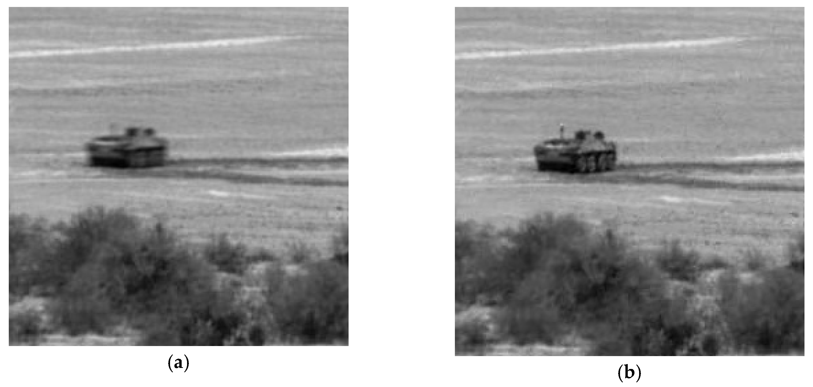
Air turbulence can seriously distort image contents and consequently can negatively affect target detection and classification performance in video surveillance [1,2,3,4]. Figure 1 shows the impact of air turbulence on video quality. All the fine features of the tower are smeared. In the past, researchers have developed numerous algorithms to mitigate turbulence effects [5,6,7,8,9,10,11,12,13] among which there are simultaneous turbulence mitigation and super-resolution (SR) algorithms [8,9]. In recent years, there are also new SR algorithms using deep learning approaches [14,15]. Combining SR with some turbulence mitigation only algorithm is of interest to the community as well.

In the aforementioned turbulence mitigation studies, researchers used simulated and real turbulence videos for demonstrations. For real videos, it is difficult to assess which algorithm is performing better because of lack of ground truth. Hence, most of the time, subjective evaluations are used, which may not be consistent in the sense that some methods with close performance may be difficult to differentiate by humans. For simulated turbulence videos, objective metrics can be generated to compare different algorithms.

In [16], a blind video quality assessment metric known as the Video Intrinsic Integrity and Distortion Evaluation Oracle (VIIDEO) was developed. However, it was tailored towards assessing compressed video quality. At this time, there does not seem to exist a consistent blind video quality assessment tool for evaluating different turbulence mitigation algorithms. In [11], a blind video quality assessment tool was mentioned. However, the code is not available to the public. In [17,18], blind video quality assessment methods were proposed for videos containing natural scenes without air turbulence. In [19], the authors compared three air turbulence mitigation algorithms. One idea uses a reference marker in the scene and this may not be practical because many videos with air turbulence are recorded in the wild.

In this paper, a new blind video quality metric for assessing different turbulence mitigation algorithms is proposed. First, given a video containing turbulence or a video that is already turbulence mitigated, one can apply existing blind still image quality assessment metrics such as Perception-based Image Quality Evaluator (PIQE) [20] and Blind/Referenceless Image Spatial Quality Evaluator (BRISQUE) [21] to assess the intra-frame spatial quality. PIQE and BRISQUE are well-known tools that can meet this intra-frame spatial quality assessment need. In this paper, the proposed metric will be utilizing BRISQUE as it was found to behave more consistently with visual inspection. Second, in order to capture the inter-frame fluctuations due to turbulence, an inter-frame root mean square error (IFRMSE) metric is proposed, which simply computes the RMSE between two neighboring frames and then take the average of all the RMSE of the frame pairs in the video. The intuition behind IFRMSE is that there are random fluctuations due to turbulence between the same pixels of different frames. If the IFRMSE is small, then turbulence effect should be small as well. Third, a hybrid metric that computes the geometric mean of the intra-frame scores and the inter-frame scores is proposed. As a result, both the intra- and inter-frame qualities have been taken into account. The proposed blind metric is in sharp contrast to the BRISQUE metric, which does not explicitly consider inter-frame fluctuations.

Here, several research questions are addressed. First, is the proposed hybrid blind video quality metric consistent with subjective evaluation results? Several turbulence mitigation algorithms in the literature were investigated, as well as the combination of those algorithms with a deep learning-based SR algorithm known as Zooming Slow Motion (ZSM) [22]. This question is important for assessing some algorithms that have very close turbulence mitigation performance. Second, can the use of additional alignment and registration techniques alongside the well-known method CLEAR [11] improve air turbulence mitigation? Third, is the existing blind video quality metric known as VIIDEO [16] suitable for assessing turbulence mitigation algorithms? Answering this will motivate new research in blind video quality assessment specifically for turbulence mitigation.

The contributions of this paper are as follows:

▪

A new blind video quality assessment metric specifically for assessing turbulence mitigation algorithms is proposed. The new metric combines both intra-frame and inter-frame qualities in videos. This metric is consistent with subjective evaluations, meaning that the new metric can help differentiate algorithms that are too close in visual inspection. Hence, the first question raised earlier is answered.

▪

The use of additional alignment and registration techniques are demonstrated to visually improve videos with air turbulence. This answers the second question raised earlier.

▪

This metric is compared with an existing metric and observed that the previous metric in [16] is not suitable for assessing turbulent mitigation algorithms. This answers the third question above.

The remainder of this paper is organized as follows. In Section 2, a few representative and recent turbulence mitigation methods are summarized. Relevant works in the field of blind quality assessment, air turbulence mitigation, and super resolution are described. In Section 3, the proposed blind video quality assessment metric and a workflow for performing air turbulence mitigation are explained in detail. Section 4 showcases the experimental results of this workflow and metric on 12 videos. In Section 5, a few concluding remarks and future directions are mentioned.

2. Related Works

2.1. Turbulence Mitigation Approaches

This section gives a glimpse of some representative papers in turbulent mitigation. It is not meant for an exhaustive literature survey. Moreover, since the focus is on assessing different turbulence mitigation algorithms and not on the advancement of those algorithms, some algorithms may not be included in the experiments.

2.1.1. Complex Wavelet Fusion for Atmospheric Turbulence

As shown in Figure 2, Complex waveLEt fusion for Atmospheric tuRbulence (CLEAR) consists of four key modules [11]: frame selection, image registration, image fusion, and image deblurring. There are some key parameters to be aware of in CLEAR. Frame selection is an essential parameter to turn on in order to stabilize frames where there might be significant motion. Once this is active, the results drastically improve as can be seen in Figure 3. The number of frames used is also an integral parameter to fine-tune. The number of frames used can improve the quality of the air turbulence removal. However, if there are too many frames with motion, there can be significant motion blurring. For the case in Figure 3, 10 frames are used. Another key aspect of CLEAR is the region of interest (ROI) selector. This allows users to specify a particular bounding box location of their subjective ROI. When used, this ROI selector significantly improves the registration portion of CLEAR, as can be seen below. This is especially useful when there is a particular object in the frame that is of interest to the user, as is the case with the vehicles in the SENSIAC dataset [23].

2.1.2. A Recent Turbulence Mitigation Approach Using Image Reconstruction

The approach proposed by Mao et al. [13] makes some decent improvements to previous air turbulence mitigation methods. First, they improve on previous methods by implementing a new way to generate reference frames, which is discussed in detail in Section 3.1. Second, they implement a geometric and sharpness metric to create the lucky frame, which is a frame with least distortion. Finally, they implement a novel blind deconvolution algorithm.

2.2. Video Super-Resolution (VSR)

In recent research [24], two video super-resolution algorithms were compared. The Zoom Slow-Motion (ZSM) Algorithm [22] for video super-resolution performed better than the Dynamic Upsampling Filter (DUF) approach [17]. As such, only ZSM is used within the experiments in this paper. The objective is to investigate whether or not VSR can help mitigate air turbulence due to the fact that VSR normally uses multiple frames together for resolution improvement. The use of multiple frames has some inherent deblurring effects to reduce air turbulence.

ZSM can be broken down into three key components: feature temporal interpolation network, a deformable convolutional long short-term memory (ConvLSTM) network, and a deep construction network [22]. The feature temporal interpolation network is used to interpolate missing temporal information between the input low resolution frames. Next, the deformable ConvLSTM is used to align and aggregate the temporal information together. Lastly, the deep construction network predicts and generates the super resolution upsampled video frames. This overall architecture is outlined in Figure 4.

2.3. Blind Metrics to Assess Turbulence Mitigation Algorithms

2.3.1. PIQE

PIQE is a blind spatial quality assessment metric [20]. The input image is first normalized and split into blocks. Each block is then fed into a distortion estimator. These block scores are then pooled together and a final quality score is outputted. The lower the score, the better quality the image is. MATLAB has a built-in function for computing PIQE [25].

2.3.2. BRISQUE

BRISQUE is a no-reference image quality assessment metric [21]. It first extracts natural scene statistics and then calculates several feature vectors. Using those features and statistics in a Support Vector Machine (SVM), it then predicts an image quality score. The lower the score the better quality the image is. No custom fitting was done for this model. There is a MATLAB function for computing BRISQUE [26].

3. Methods

3.1. Using Reference Frame Only for Turbulence Mitigation

One way to potentially mitigate air turbulence is by using a new approach to generate a reference frame, which is important for image alignment. The authors of [13] outline this approach in the equation below. For each given patch in a frame, a search is performed on a set number of subsequent frames and previous frames for that same patch in a search window slightly larger than the patch size. There is an assumption that there is no significant motion of objects between consecutive frames. Based on the Euclidian distance of the patch in the subsequent and previous frames, the best possible match for the patch at the current frame is found. Afterwards, a weighted average of the patches is used to generate a new reference frame ${\widehat{y}}_{ref}\left(r,t\right)$.

$${\widehat{y}}_{ref}\left(r,t\right)=\frac{{\sum }_{\Delta t\in {\mathsf{\Omega }}_t}{w}_{r,t}\left(\Delta t\right)y\left(r,t+\Delta t\right)}{{\sum }_{\Delta t\in {\mathsf{\Omega }}_t}{w}_{r,t}\left(\Delta t\right)}$$

(1)

where r denotes the given patch center location, ${\mathsf{\Omega }}_t$ is a search window surrounding the current patch, $\Delta t$ denotes the shift in terms of pixels between the current patch and a patch in the search window, and ${\omega }_{r,t}$ represents the weighting of a given patch and is the inverse of Euclidean distance between the current patch and a given patch within the search window.

Figure 5 illustrates how to generate a sequence of reference (Ref) video. For a group of N frames, Equation (1) is applied to generate one reference frame. The window of frames shifts to the right by one and then another reference frame is generated. This process repeats for the whole video.

Previous approaches, such as averaging the frames [8,9,10], do not work as well as this approach. If there is air turbulence or even motion in the frames, simply averaging the frames will only smear the moving objects. This new approach to generating reference frames creates a much smooth frame that maintains the edges and shapes of moving objects. Figure 6 shows a comparison of the two different approaches and the advantages offered by the patch-based reference generation.

3.2. Proposed Workflow for Air Turbulence Mitigation

Instead of independently using reference frame alignment, CLEAR, or ZSM, these can be used in conjunction with one another to further improve image quality of air turbulent videos. The following order of algorithms are proposed: reference frame alignment, CLEAR, ZSM. As shown above in Section 3.1, the reference frame alignment can provide crisper frames. In theory, this will make objects sharper even before the air turbulence mitigation. The final step would be to apply ZSM to the output of CLEAR. Although ZSM is a super resolution method, it also performs image fusion. It does so by aligning neighboring sequences of frames. These alignments further improve the quality of the frames. In essence, this proposed workflow utilizes a variety of registration and alignment methods to perform more holistic air turbulence mitigation.

3.3. Proposed Simple Inter-Frame RMSE (IFRMSE) Metric for Inter-Frame Quality Assessment

Simply using a blind quality assessment metric on a still frame does not give a holistic representation of the performance of different turbulence mitigation algorithms in a video with turbulence. The issue with air turbulence is not the noise in the individual frame but the noise that randomly changes from frame to frame due to air turbulence. In order to better assess air turbulence mitigation, a metric needs to measure the consistency of pixels across frames.

One simple way to measure the consistency is to take the RMSE at each pixel location between frame pairs. Using an inter-frame RMSE to measure the effect of air turbulence across frames is proposed. For every frame pair, the RMSE between the current frame, F_i, and the subsequent frame, F_i+1 is taken. That is, the inter-frame RMSE for frame pair i is defined as

$$IFRMS{E}_i{}_{ }=\sqrt{\frac{{\sum }_{j=1}^N{\left(F_{i,j}-F_{i+1,j}\right)}^2}{N}}$$

(2)

where F_i,j denotes the jth pixel in frame F_i and N is the total number of pixels in a frame.

To assess the video quality, it is necessary to compute IFRMSE values from multiple frame pairs in order to reduce the statistical variations. For a video sequence, v, of n frames, there will be n−1 frame pairs. The following equation calculates the mean of the IFRMSEs as

$$IFRMS{E}_{ }=\frac{{\sum }_{i=1}^{n-1}IFRMS{E}_i }{n-1}$$

(3)

A few cautionary notes are needed. First, if the camera moves, then an image registration step is needed between the two frames in a frame pair. The aligned images can then be used for computing the IMRMSE. Second, if there are moving objects in the videos, the number and size of the moving objects may limit the effectiveness of the metric. If the number of pixels related to the moving objects is a small percentage (<5%) of the total number of pixels in a frame, then it should be alright to proceed with the calculation of IFRMSE. However, if the number of moving pixels due to moving objects is too large (10% or more), then one must apply optical flow techniques to determine those large moving objects and then exclude them in the computation of IFRMSE.

3.4. Proposed Hybrid Blind Video Quality Assessment Metric

One shortcoming of the IFRMSE metric is that it does not measure the actual quality of individual frames. For example, in a case where the image quality in a video was poor and the frames were consistently poor across the sequence, the IFRMSE metric would be quite low (indicating a high-quality video) even though there is no air turbulence. Such a case can happen to a highly compressed video in which all frames have poor quality due to compression. To overcome this shortcoming of IFRMSE, one can combine the score with one of the blind quality assessment scores. More specifically, take the geometric mean of the IFRMSE metric over many frame pairs and the intra-frame metric BRISQUE scores over many frames to generate a hybrid score. That is, the hybrid metric is given by

$$H_{IB}=\sqrt{\left(IFRMSE\right)\ast BRISQUE}$$

(4)

Experiments were conducted with PIQE, but could not get consistent results. Hence, only Equation (4) is used in the experiments. PIQE could be used as a replacement for BRISQUE for certain datasets if needed.

The geometric mean has a few advantages over the arithmetic mean. First, in dealing with metrics from different domains, it will be a good practice to use geometric mean. This will be fair to each of the contributing metrics in the product. That is, a given percentage change in any of the two metrics has the same effect on the product. For example, a 10% change in intra-frame metric from 0.1 to 0.11 has the same effect on the overall geometric mean as a 10% change in inter-frame metric from 0.5 to 0.55. Second, the geometric mean can better handle large dynamic ranges of two metrics. For instance, if the intra-frame metric is 0.01 and inter-frame is 0.9, the geometric of the two will be 0.3, but the arithmetic mean will give 0.455. As a result, the arithmetic mean will favor the metric that has large values.

The hybrid metric above should be more indicative of air turbulence mitigation across videos. Additionally, the metric can be used on datasets without having a ground truth video. This makes it more flexible in real-world scenarios where the ground truth video may not be available or possible to attain.

One might think that the proposed metric in Equation (4) is too simple and lacks novelty. Indeed, the proposed blind metric is simple and intuitive. However, there were no similar approaches in the literature. Moreover, scientific discoveries are usually incremental in nature. In this sense, the proposed metric is contributing new knowledge to the literature.

It is worth mentioning some differences between VIIDEO and the proposed metric. First, the VIIDEO metric is a patch-based method. It computes the local contrast of each patch across multiple frames. The metric is simpler in that one only needs to compute the RMSE between neighboring frames without using patches. Second, VIIDEO does not have a spatial only metric for assessing the image quality in each frame whereas the proposed approach has an explicit spatial quality component.

4. Experimental Results

Here, an overview of the 12 video datasets containing air turbulence as well as assessment results are presented. Eleven of them are well-known in the literature.

4.1. Dataset and Workflow Overview

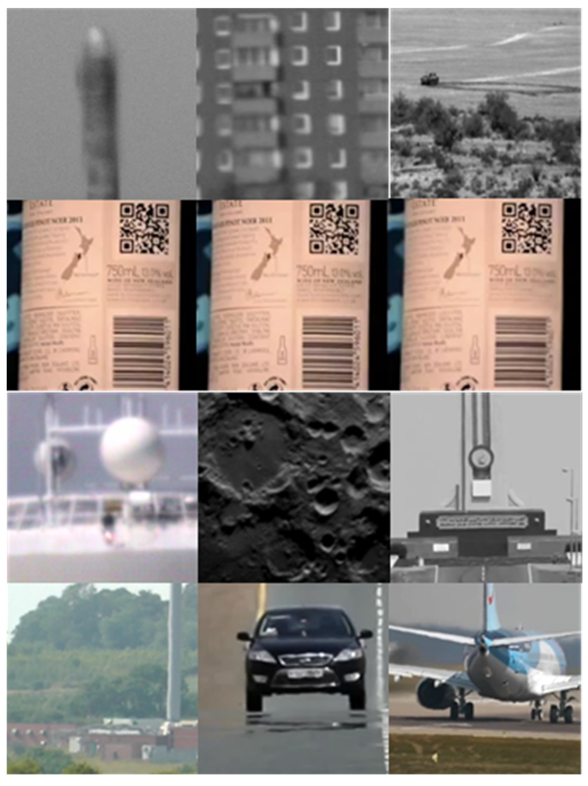
A combination of simulated data and real video datasets were used to validate both the blind quality assessment metric as well as the proposed air turbulence mitigation workflow.

Table 1. Summary of video datasets used in experiments. “Wild” means that a video was taken from an actual scene.

Video	Wild	Moving	Size	Frames
Chimney	No	No	256 × 256	50
Building	No	No	256 × 256	50
SENSIAC	Yes	Yes	256 × 256	50
Barcode #1	No	No	215 × 215	50
Barcode #2	No	No	215 × 215	50
Barcode #3	No	No	215 × 215	50
Watertower	Yes	No	225 × 225	50
Moon	Yes	No	256 × 256	50
Monument	Yes	No	256 × 256	50
Secret base	Yes	No	256 × 256	100
Mirage	Yes	Yes	256 × 256	100
Airport	Yes	Yes	256 × 256	100

and Figure 7 summarize those videos. Barcode #1–#3 have different levels of turbulence. If a video is not wild it is a simulated video. Moving refers to whether the object or camera is moving in the video. This is an important distinction because the motion of the object or camera can interfere with blind quality measurements.

For each video, the following workflows are compared:

▪

Raw: This is the raw video with turbulence.

▪

Ref: This is the video generated by using the method described in Section 3.1

▪

Raw + CLEAR: This is the turbulence mitigated video using CLEAR.

▪

Ref + CLEAR: This is the video generated by applying CLEAR to the Ref video.

▪

Raw + CLEAR + ZSM: This is the video generated by applying ZSM to the Raw + CLEAR video.

▪

Ref + CLEAR + ZSM: This is the video generated by applying ZSM to the Ref + CLEAR video.

In the following tables showcasing the experimental results, the IFRMSE and BRISQUE scores are the average score across the frames used in a particular video. This is done to give a more holistic view of how a particular method performs over the course of a video.

Videos comparing the various methods can be found in the following link: https://rb.gy/wdwxh7 (accessed on 16 September 2021). Readers are encouraged to watch those videos and check the visual performance of different methods.

4.2. Hybrid Blind Quality Assessment Results

As one can observe from

Table 2. IFRMSE, BRISQUE, and H_IB scores for 12 videos.

	SENSIAC				Building				Chimney
Methods	IFRMSE	BRISQUE	$H_{IB}$	Rank	IFRMSE	BRISQUE	$H_{IB}$	Rank	IFRMSE	BRISQUE	$H_{IB}$	Rank
Raw	4.39	23.48	10.15	6	1.2602	45.3415	7.5592	6	3.73	52.81	14.04	6
Ref	3.15	25.61	8.98	5	1.152	46.8207	7.3442	5	3.21	38.69	11.14	5
Raw + CLEAR	1.77	18.73	5.76	4	0.6076	39.5277	4.9008	4	1.87	45.81	9.26	4
Ref + CLEAR	1.26	21.14	5.16	3	0.3452	38.4578	3.6434	3	1.22	44.97	7.41	2
Raw + CLEAR +ZSM	1.24	19.33	4.9	2	0.3108	38.0239	3.4376	2	1.66	37.16	7.85	3
Ref+ CLEAR +ZSM	0.88	21.54	4.35	1	0.1711	38.5113	2.5666	1	1.21	30.34	6.06	1
	Water Tower				Moon				Monument
Methods	IFRMSE	BRISQUE	$H_{IB}$	Rank	IFRMSE	BRISQUE	$H_{IB}$	Rank	IFRMSE	BRISQUE	$H_{IB}$	Rank
Raw	1.5043	53.1893	8.945	6	1.2602	45.3415	7.5592	6	2.7772	42.4074	10.8523	6
Ref	1.4077	53.9155	8.7119	5	1.152	46.8207	7.3442	5	2.6891	42.9818	10.751	5
Raw + CLEAR	0.5673	46.6926	5.1469	3	0.6076	39.5277	4.9008	4	1.1373	36.7082	6.4613	4
Ref + CLEAR	0.5228	51.5237	5.19	4	0.3452	38.4578	3.6434	3	0.8158	36.9296	5.4887	3
Raw + CLEAR +ZSM	0.2781	44.3203	3.5107	1	0.3108	38.0239	3.4376	2	0.6776	37.11	5.0147	2
Ref+ CLEAR +ZSM	0.2562	52.5189	3.668	2	0.1711	38.5113	2.5666	1	0.4475	37.4448	4.0934	1
	Barcode #1				Barcode #2				Barcode #3
Methods	IFRMSE	BRISQUE	$H_{IB}$	Rank	IFRMSE	BRISQUE	$H_{IB}$	Rank	IFRMSE	BRISQUE	$H_{IB}$	Rank
Raw	3.577	40.919	12.0983	5	4.8176	41.15	14.0799	6	5.3736	46.1176	15.7423	5
Ref	3.4943	41.977	12.1112	6	4.7447	41.7146	14.0685	5	5.2976	46.9052	15.7634	6
Raw + CLEAR	1.2879	29.5506	6.1691	4	1.4656	29.5351	6.5793	4	1.874	30.9387	7.6145	4
Ref + CLEAR	0.7784	27.1397	4.5964	3	1.0033	29.3368	5.4254	3	1.3501	35.9165	6.9636	3
Raw + CLEAR +ZSM	0.7413	26.2908	4.4145	2	0.794	27.6011	4.6815	2	0.9427	32.9359	5.572	2
Ref+ CLEAR +ZSM	0.4172	27.2035	3.3691	1	0.5216	28.7136	3.8699	1	0.6933	37.7056	5.1128	1
	Base				Mirage				Airport
Methods	IFRMSE	BRISQUE	$H_{IB}$	Rank	IFRMSE	BRISQUE	$H_{IB}$	Rank	IFRMSE	BRISQUE	$H_{IB}$	Rank
Raw	1.8141	38.0121	8.3041	6	5.3942	37.9655	14.3106	6	3.0487	49.477	12.2817	6
Ref	1.7372	39.4329	8.2765	5	5.2914	37.0854	14.0084	5	2.9227	50.3713	12.1334	5
Raw + CLEAR	0.5584	37.188	4.5571	4	3.1875	33.6723	10.36	4	2.1779	37.0528	8.9832	4
Ref + CLEAR	0.5055	35.9097	4.2605	3	2.94	33.3768	9.906	3	2.0918	38.0481	8.9214	3
Raw + CLEAR +ZSM	0.2957	35.6662	3.2473	2	1.4926	33.3824	7.0589	1	1.9084	38.3016	8.5496	2
Ref+ CLEAR +ZSM	0.2633	34.3795	3.0084	1	1.5584	34.7729	7.3614	2	1.8277	39.3859	8.4845	1

that the results for the rankings of hybrid score of BRISQUE and the proposed IFRMSE are very consistent. Raw and Ref methods are always ranked 5–6, CLEAR based methods are ranked 3–4, and ZSM methods are always ranked 1–2. These rankings are strongly aligned with visual inspection of various outputs from each method.

4.2.1. Reference Alignment vs. Raw

Using the reference alignment produces a slight improvement in IFRMSE over the Raw in all videos except for ‘Barcode #3′. Although the difference in IFRMSE is not very significant between the Raw and Ref, the effects are amplified when used in conjunction with CLEAR and ZSM. CLEAR and ZSM have drastrically lower IFRMSE when using Ref based frames than just the Raw for most videos. BRISQUE scores across the Raw and Ref methods are fairly consistent, with only the ‘Chimney’ sequence as an exception. This makes sense as BRISQUE does not take into account inter-frame variability.

4.2.2. Effects of CLEAR and ZSM

If CLEAR is respectively applied to the output of the Raw and Ref, there is a significant improvement in the IFRMSE and therefore the H_IB as well. When CLEAR removes the air turbulence and the frame contents become stable, there is significantly less motion between frames. The scores for any method utilizing CLEAR are significantly lower than that of its respective counterpart. This means the IFRMSE is in agreement with these visual observations in all the video datasets. CLEAR has mostly positive effects BRISQUE scores of the Raw and Ref based methods. For example, in all three ‘Barcode’ sequences there is a ~25% improvement in BRISQUE scores from the Raw and Ref to the Raw + CLEAR and Ref + CLEAR. In the Watertower and Base videos, the effects are more subtle.

When ZSM is applied to the output of the CLEAR based methods, there is another significant improvement in IFRMSE scores. Although the ZSM visual effects are subtle, the IFRMSE does indicate a significant improvement. These improvements can be attributed to the ConvLSTM module in the ZSM which temporally aligns sequences of frames. This alignment further reduces pixel fluctuations between frames. There is no consistent trend for the BRISQUE scores of ZSM based methods perhaps due to the fact that BRISQUE is not sensitive enough to notice the minor improvements from the ZSM.

4.3. Chimney and Building Videos

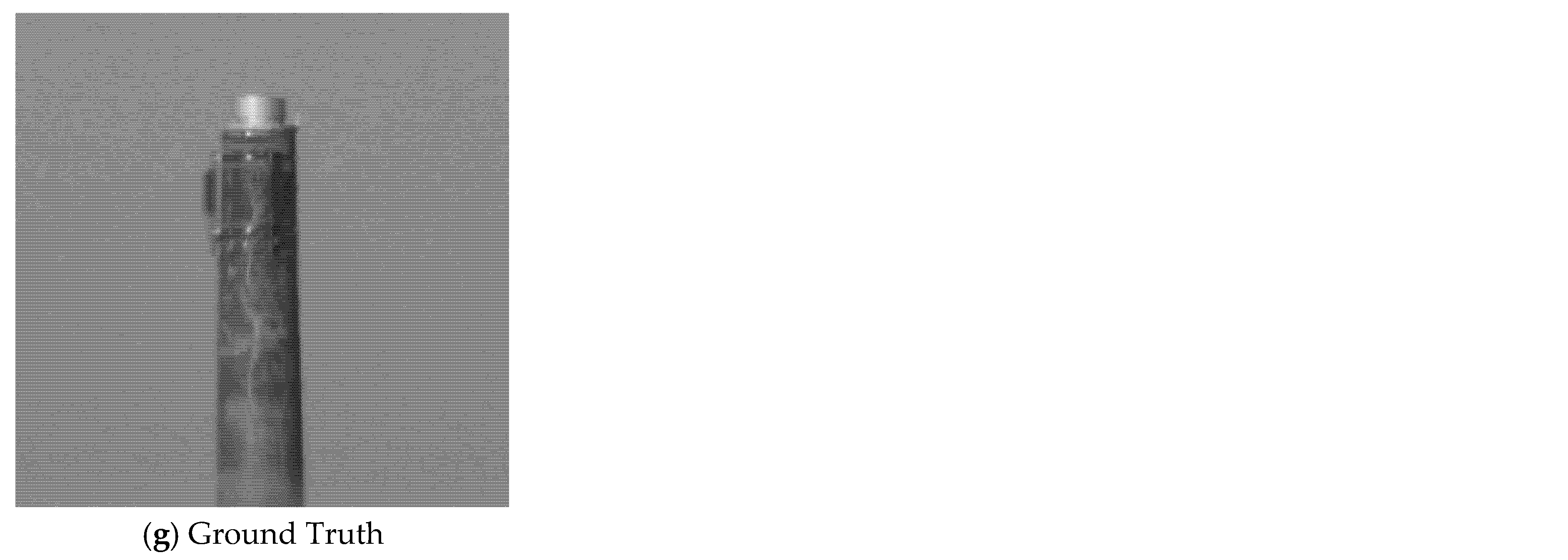
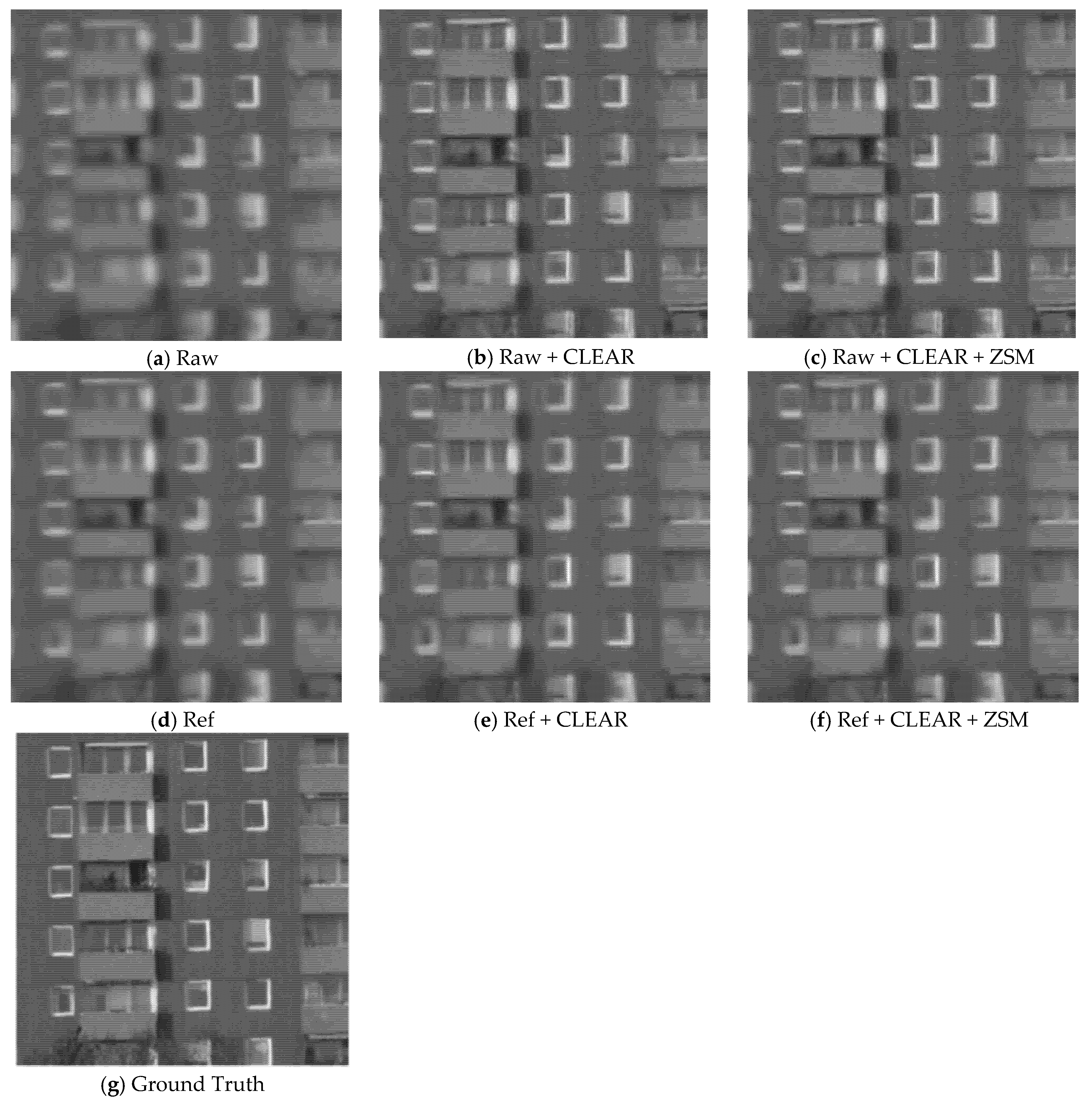
Here, there are detailed analysis of the Chimney and Building videos. Readers are encouraged to visualize these videos in the link: https://rb.gy/wdwxh7 (accessed on 16 September 2021). Snapshots of one frame from every video are shown in Figure 8 and Figure 9 for the Chimney and Building videos, respectively.

From

Table 3. Comparison of different approaches using BRISQUE, inter-frame RMSE, and hybrid metrics for the ‘Chimney’ sequence.

Methods	IFRMSE	BRISQUE	HIB	HIB Rank
Raw	3.73	52.81	14.04	6
Ref	3.21	38.69	11.14	5
Raw + CLEAR	1.87	45.81	9.26	4
Ref + CLEAR	1.22	44.97	7.41	2
Raw + CLEAR + ZSM *	1.66	37.16	7.85	3
Ref + CLEAR + ZSM *	1.21	30.34	6.06	1

* Rescaled to same size as raw when calculating metrics.

and

Table 4. Comparison of different approaches using BRISQUE, inter-frame RMSE, and hybrid metrics for the ‘Building’ sequence.

Methods	IFRMSE	BRISQUE	HIB	HIB Rank
Raw	12.67	53.88	26.13	6
Ref	5.72	53.51	17.50	5
Raw + CLEAR	3.53	48.06	13.03	4
Ref + CLEAR	2.53	51.98	11.47	3
Raw + CLEAR + ZSM *	1.85	52.34	9.84	2
Ref + CLEAR + ZSM *	1.58	41.07	8.06	1

* Rescaled to same size as raw when calculating metrics.

, Figure 8 and Figure 9, following observations can be made:

▪

The use of Ref sequence helps improve the turbulence mitigation performance. This can be seen when one compares the IFRMSE and BRISQUE scores of Raw vs. Ref, Raw + CLEAR vs. Ref + CLEAR, Raw + CLEAR + ZSM vs. Ref + CLEAR + ZSM. This is because Ref sequence provides more stable frames for image alignment, which is an important step in CLEAR.

▪

The combination of CLEAR and ZSM improves over that of using only CLEAR.

▪

The visual inspection of the various turbulence videos seems to agree with the objective metrics in Table 3 and Table 4. It is difficult to visually differentiate between the ZSM results with their non-ZSM counterparts. That is why it is important to have an objective metric to be able to better distinguish the subtle differences in the images. In the included cases, the Hybrid IFRMSE and BRISQUE metric seemed to better assess the quality of the videos.

▪

It can be observed in the videos that CLEAR greatly reduces the ‘wobbling’ of the scene suffering from significant air turbulence.

▪

Although it is difficult to determine the extent of improvement from a still image, the images do provide a general indication of the level of improvement. Figure 8 and Figure 9 below show the various methods affect the quality of individual frames.

4.4. Comparison with VIIDEO

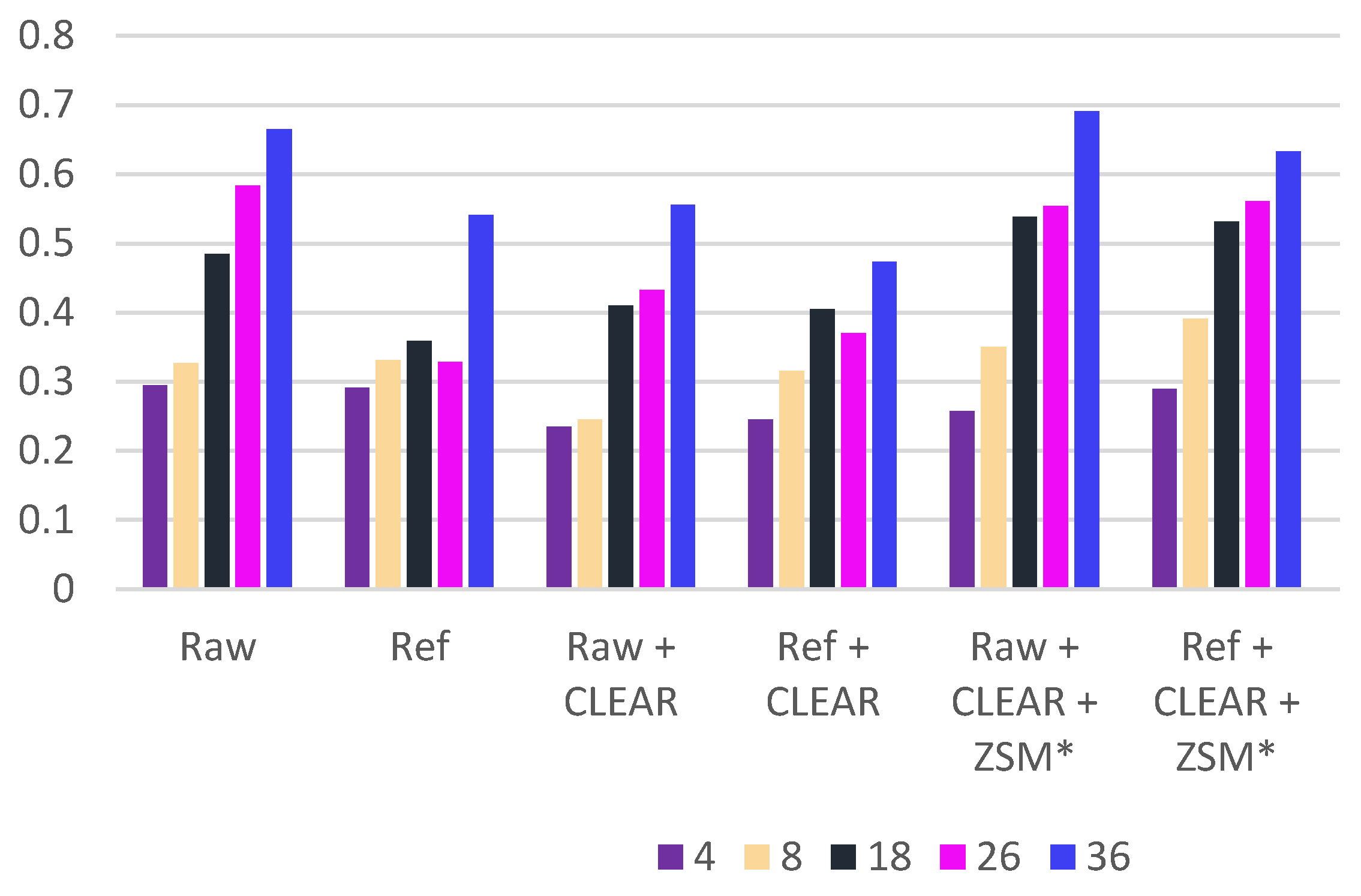
The VIIDEO metric was tested on the three videos. Initially, the ‘Building’ sequence was used to test various parameters for the metric. In particular, experiments were conducted to determine the optimal block size. From the initial study, it was found that a small block size, like 4, more accurately rates the videos. As can be seen in

Table 5. Block size selection for the ‘Building’ sequence.

Block Sizes	4		8		18		26		36
Method	VIIDEO	VIIDEO Rank	VIIDEO	VIIDEO Rank	VIIDEO	VIIDEO Rank	VIIDEO	VIIDEO Rank	VIIDEO	VIIDEO Rank
Raw	0.294	6	0.327	3	0.485	4	0.584	6	0.665	5
Ref	0.291	5	0.332	4	0.359	1	0.329	1	0.541	2
Raw + CLEAR	0.235	1	0.245	1	0.410	3	0.433	3	0.556	3
Ref + CLEAR	0.245	2	0.315	2	0.405	2	0.371	2	0.474	1
Raw + CLEAR + ZSM*	0.257	3	0.351	5	0.539	6	0.554	4	0.691	6
Ref + CLEAR + ZSM *	0.289	4	0.391	6	0.532	5	0.561	5	0.633	4

* Rescaled to same size as raw when calculating metrics.

and Figure 10, VIIDEO with a smaller block size more appropriately ranks the methods. The Raw is rated as the worst and the Raw + CLEAR is the best. These are more closely aligned with visual inspection than the rankings from the other block sizes.

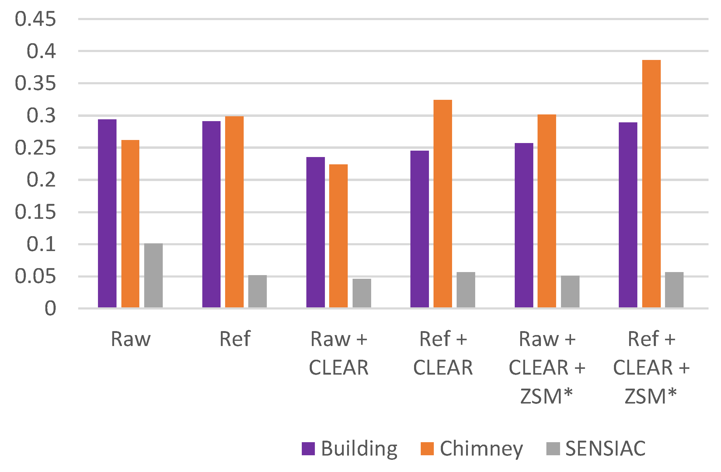
A block size of 4 was used for VIIDEO in all three videos. The VIIDEO metrics are shown in

Table 6. VIIDEO score for all three sequences.

(a) VIIDEO Metrics and Rankings for Building and Chimney Videos
	Building		Chimney
Methods	VIIDEO	VIIDEO Rank	VIIDEO	VIIDEO Rank
Raw	0.294	6	0.262	2
Ref	0.291	5	0.299	3
Raw + CLEAR	0.235	1	0.224	1
Ref + CLEAR	0.245	2	0.324	5
Raw + CLEAR + ZSM *	0.257	3	0.301	4
Ref + CLEAR + ZSM *	0.289	4	0.386	6
(b) VIIDEO metrics and rankings for the SENSIAC video
		SENSIAC
Methods		VIIDEO	VIIDEO Rank
Raw		0.101	6
Ref		0.052	3
Raw + CLEAR		0.046	1
Ref+ CLEAR		0.056	5
Raw+ CLEAR + ZSM *		0.051	2
Ref + CLEAR + ZSM *		0.056	4

* Rescaled to same size as raw when calculating metrics.

and Figure 11. There is inconsistency across the three video sequences in terms of which method performs the best. For instance, VIIDEO ranked the raw turbulence video as the second in the Chimney case, which is clearly inconsistent with subjective evaluation. Another inconsistent instance is that the Ref + CLEAR + ZSM videos were ranked 4, 6, and 4 in the Building, Chimney, and SENSIAC videos, respectively. This inconsistency indicates that VIIDEO metrics are still not robust at handling various types of distortions in videos. For example, authors in [16] found that the VIIDEO metric worked well in distinguishing between compression artifacts but did not mention their performance for other types of distortions that may arise, such as air turbulence. From the preliminary studies, one can see that the VIIDEO performance metric was inconsistent for air turbulence.

5. Conclusions

A new blind video quality metric was proposed to assess air turbulence mitigation performance in video sequences. These results were in agreement with visual inspection. Twelve commonly used videos were used to perform this validation. Experimental results showed that the metrics are consistent with subjective evaluation of videos. The experiments demonstrated the effectiveness of using CLEAR in combination with reference frame alignment and ZSM to mitigate air turbulence.

One anonymous reviewer pointed out that turbulence may be treated as shake and blurry effects and hence some denoising algorithms such as [27,28] can be used. This could be a reasonable future research topic. Another future direction is to investigate how one can adapt some blind assessment metrics, such as those in [16,29,30], to turbulence mitigated videos. Finally, there could be further research into the effects of motion within videos and how they may affect blind quality assessment metrics like IFRMSE. Some new developments in video quality assessment [31,32,33] in non-air-turbulence mitigation areas could potentially be adapted to blind image quality assessment in air turbulence videos.

References

- Kwan, C.; Budavari, B.; Ayhan, B. Comparing Video Activity Classifiers within a Novel Framework. Electronics 2020, 9, 1545. [Google Scholar] [CrossRef]
- Ayhan, B.; Kwan, C.; Budavari, B.; Larkin, J.; Gribben, D.; Li, B. Video Activity Detection Under Different Rhythms. IEEE Access 2020, 8, 191997–192008. [Google Scholar] [CrossRef]
- Kwan, C.; Chou, B.; Yang, J.; Tran, T. Deep Learning based Target Tracking and Classification Directly in Compressive Measurement for Low Quality Videos. Signal Image Process. Int. J. 2019, 10, 9–29. [Google Scholar] [CrossRef]
- Kwan, C.; Budavari, B. Enhancing Small Moving Target Detection Performance in Low-Quality and Long-Range Infrared Videos Using Optical Flow Techniques. Remote Sens. 2020, 12, 4024. [Google Scholar] [CrossRef]
- Gibson, K.B.; Nguyen, T.Q. An Analysis and Method for Contrast Enhancement Turbulence Mitigation. IEEE Trans. Image Process. 2014, 23, 3179–3190. [Google Scholar] [CrossRef]
- Lau, C.P.; Lai, Y.H.; Lui, L.M. Restoration of atmospheric turbulence-distorted images via RPCA and quasiconformal maps. Inverse Problems. 2019, 35, 074002. [Google Scholar] [CrossRef] [Green Version]
- Zhu, X.; Milanfar, P. Removing atmospheric turbulence via space invariant deconvolution. IEEE Trans. Pattern Anal. Mach. Intell. 2013, 35, 157–170. [Google Scholar] [CrossRef] [Green Version]
- Hardie, R.C.; Rucci, M.A.; Karch, B.K.; Dapore, A.J.; Droege, D.R.; French, J.C. Fusion of interpolated frames superresolution in the presence of atmospheric optical turbulence. Opt. Eng. 2019, 58, 083103. [Google Scholar] [CrossRef] [Green Version]
- Droege, D.R.; Hardie, R.C.; Allen, B.S.; Dapore, A.J.; Blevins, J.C. A Real-Time Atmospheric Turbulence Mitigation and Super-Resolution Solution for Infrared Imaging Systems; International Society for Optics and Photonics: Bellingham, WA, USA, 2012; Volume 8355, p. 83550. [Google Scholar]
- Hardie, R.C.; Rucci, M.A.; Dapore, A.J.; Karch, B.K. Block matching and Wiener filtering approach to optical turbulence mitigation and its application to simulated and real imagery with quantitative error analysis. Opt. Eng. 2017, 56, 071503. [Google Scholar] [CrossRef]
- Anantrasirichai, N.; Achim, A.; Kingsbury, N.G.; Bull, D.R. Atmospheric turbulence mitigation using complex wavelet-based fusion. IEEE Trans. Image Process. 2013, 22, 2398–2408. [Google Scholar] [CrossRef] [Green Version]
- Anantrasirichai, N.; Achim, A.; Bull, D.R. Atmospheric Turbulence Mitigation for Sequences with Moving Objects Using Recursive Image Fusion. In Proceedings of the 25th IEEE International Conference on Image Processing (ICIP), Athens, Greece, 7–10 October 2018; pp. 2895–2899. [Google Scholar]
- Mao, Z.; Chimitt, N.; Chan, S.H. Image Reconstruction of Static and Dynamic Scenes Through Anisoplanatic Turbulence. IEEE Trans. Comput. Imaging 2020, 6, 1415–1428. [Google Scholar] [CrossRef]
- Jo, Y.; Oh, S.W.; Kang, J.; Kim, S.J. Deep video super-resolution network using dynamic upsampling filters without explicit motion compensation. In Proceedings of the IEEE Conference on Computer Vision and Pattern Recognition, Salt Lake City, UT, USA, 18–23 June 2018; pp. 3224–3232. [Google Scholar]
- Xiang, X. GitHub. 2020. Available online: Github.com/Mukosame/Zooming-Slow-Mo-CVPR-2020 (accessed on 16 September 2021).
- Mittal, A.; Saad, M.A.; Bovik, A.C. A completely blind video integrity oracle. IEEE Trans. Image Process. 2015, 25, 289–300. [Google Scholar] [CrossRef]
- Korhonen, J. Two-Level Approach for No-Reference Consumer Video Quality Assessment. IEEE Trans. Image Process. 2019, 28, 5923–5938. [Google Scholar] [CrossRef]
- Li, D.; Jiang, T.; Jiang, M. Quality Assessment of In-the-Wild Videos. In Proceedings of the 27th ACM International Conference on Multimedia (MM ’19), Nice, France, 21–25 October 2019. [Google Scholar]
- Kozacik, S.T.; Paolini, A.L.; Sherman, A.; Bonnett, J.L.; Kelmelis, E.J. Comparison of turbulence mitigation algorithms. Opt. Eng. 2017, 56, 071507. [Google Scholar] [CrossRef]
- Venkatanath, N.; Praneeth, D.; Chandrasekhar, B.M.; Channappayya, S.S.; Medasani, S.S. Blind Image Quality Evaluation Using Perception Based Features. In Proceedings of the 21st National Conference on Communications (NCC), Mumbai, India, 27 February–1 March 2015; IEEE: Piscataway, NJ, USA, 2015. [Google Scholar]
- Mittal, A.; Moorthy, A.K.; Bovik, A.C. No-Reference Image Quality Assessment in the Spatial Domain. IEEE Trans. Image Process. 2012, 21, 4695–4708. [Google Scholar] [CrossRef]
- Xiang, X.; Tian, Y.; Zhang, Y.; Fu, Y.; Allebach, J.P.; Xu, C. Zooming Slow-Mo: Fast and Accurate One-Stage Space-Time Video Super-Resolution. In Proceedings of the IEEE/CVF Conference on Computer Vision and Pattern Recognition, Seattle, WA, USA, 13–19 June 2020; pp. 3370–3379. [Google Scholar]
- SENSIAC Dataset. Available online: https://www.news.gatech.edu/2006/03/06/sensiac-center-helps-advance-military-sensing (accessed on 12 November 2020).
- Kwan, C.; Budavari, B. A High Performance Approach to Detecting Small Targets in Long Range Low Quality Infrared Videos. Signal Image Video Process. 2021, 1–9. [Google Scholar] [CrossRef]
- Perception-based Image Quality Evaluator (PIQE). Available online: https://www.mathworks.com/help/images/ref/piqe.html (accessed on 12 November 2020).
- Blind/Referenceless Image Spatial Quality Evaluator (BRISQUE). Available online: https://www.mathworks.com/help/images/ref/brisque.html (accessed on 12 November 2020).
- Ouahabi, A. A review of wavelet denoising in medical imaging. In Proceedings of the 8th International Workshop on Systems, Signal Processing and their Applications (WoSSPA), Algiers, Algeria, 12–15 May 2013; pp. 19–26. [Google Scholar]
- Srivastava, M.; Anderson, C.L.; Freed, J.H. A New Wavelet Denoising Method for Selecting Decomposition Levels and Noise Thresholds. IEEE Access 2016, 4, 3862–3877. [Google Scholar] [CrossRef]
- Ferroukhi, M.; Ouahabi, A.; Attari, M.; Habchi, Y.; Taleb-Ahmed, A. Medical Video Coding Based on 2nd-Generation Wavelets: Performance Evaluation. Electronics 2019, 8, 88. [Google Scholar] [CrossRef] [Green Version]
- Gao, X.; Gao, F.; Tao, D.; Li, X. Universal blind image quality assessment metrics via natural scene statistics and multiple kernel learning. IEEE Trans Neural Netw. Learn. Syst. 2013, 24, 2013–2026. [Google Scholar]
- Yang, J.; Liu, T.; Jiang, B.; Lu, W.; Meng, Q. Panoramic Video Quality Assessment Based on Non-Local Spherical CNN. IEEE Trans. Multimed. 2021, 23, 797–809. [Google Scholar] [CrossRef]
- Yang, J.; Zhao, Y.; Liu, J.; Jiang, B.; Meng, Q.; Lu, W.; Gao, X. No Reference Quality Assessment for Screen Content Images Using Stacked Autoencoders in Pictorial and Textual Regions. In IEEE Transactions on Cybernetics; IEEE: Piscataway, NJ, USA. [CrossRef]
- Yang, J.; Bian, Z.; Zhao, Y.; Lu, W.; Gao, X. Full-Reference Quality Assessment for Screen Content Images Based on the Concept of Global-Guidance and Local-Adjustment. IEEE Trans. Broadcasting 2021, 67, 696–709. [Google Scholar] [CrossRef]
Figure 1.
Video frames with and without air turbulence effects. (a) A frame with turbulence; (b) A frame without turbulence.
Figure 2.
CLEAR architecture [11]. Frame selection generates lucky regions which are referring to image patches that are least affected by air turbulence. Details can be found in [11].
Figure 3.
Comparison of no frame selection vs. frame selection for CLEAR algorithm. (a) No frame selection; (b) with frame selection.
Figure 4.
ZSM architecture [22].
Figure 5.
Generation of the Ref sequence. N = 7 in this example.
Figure 6.
Comparison of generating reference frames for image alignment. (a) Averaging frame results; (b) Result using the approach in [13].
Figure 7.
Sample frames from each video. First row: Chimney, Building, SENSIAC. Second row: Barcode #1–#3. Third row: Water tower, Moon, Monument. Fourth row: Secret base, Mirage, Airport.
Figure 8.
Method comparisons of the ‘Chimney’ sequence. (a) Raw; (b) Raw + CLEAR; (c) Raw + CLEAR + ZSM; (d) Ref; (e) Ref + CLEAR; (f) Ref + CLEAR + ZSM; (g) Ground truth.
Figure 9.
Method comparison of the ‘Building’ sequence. (a) Raw; (b) Raw + CLEAR; (c) Raw + CLEAR + ZSM; (d) Ref; (e) Ref + CLEAR; (f) Ref + CLEAR + ZSM; (g) Ground truth.
Figure 10.
Bar charts depicting the contents in Table 5.
Figure 11.
Bar charts depicting the contents in Table 6.