
Design & Optimization of Large Cylindrical Radomes with Subcell and Non-Orthogonal FDTD Meshes Combined with Genetic Algorithms

 ,
,  , and
, and
Abstract
:1. Introduction
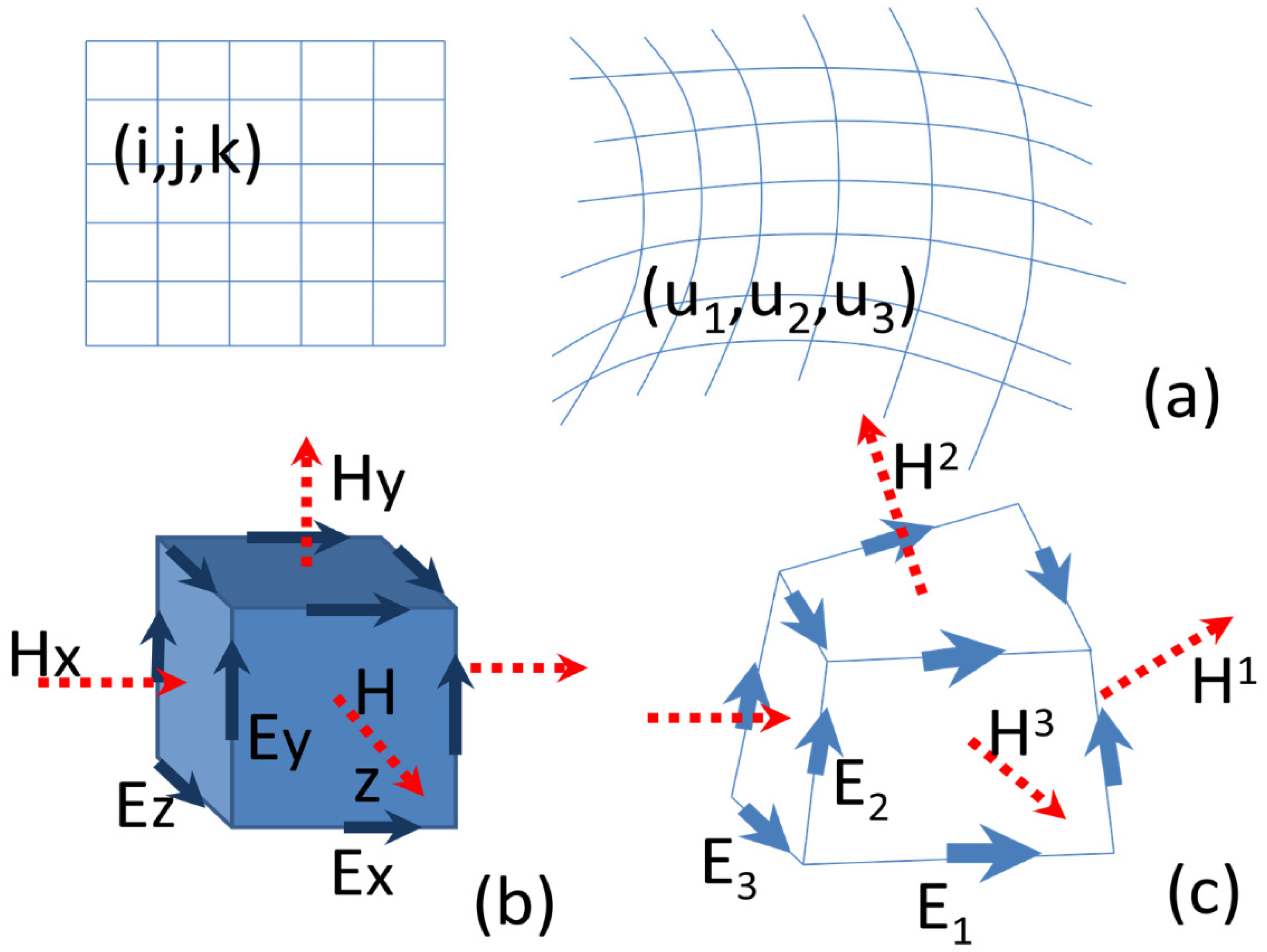
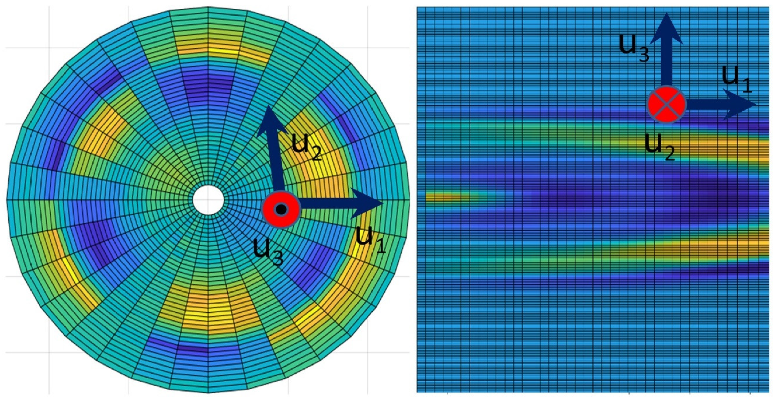
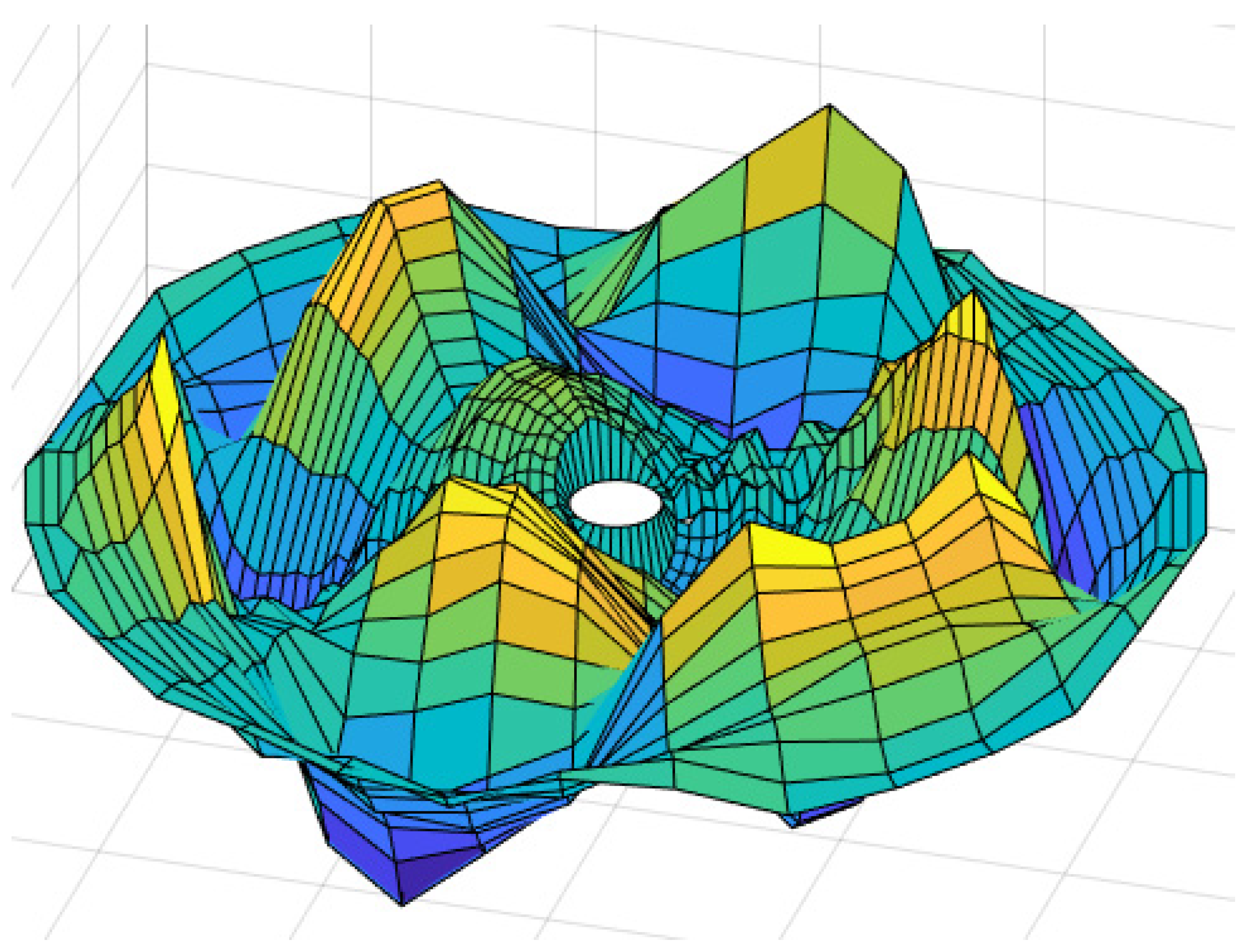
2. The Curvilinear FDTD
- -
- Covariant and contravariant fields at each cell node
- -
- Metric tensor gij, is a 3 × 3 symmetrical matrix defined each cell to carry out contravariant to covariant transformation
- -
- Calculation effort in terms of CPU/GPU in curvilinear FDTD
- -
- Contravariant to covariant transformation using the metric tensor gij
- -
- Initial values: Variables are initialized and constant parameters are defined.
- -
- Contravariant field components Ei are obtained using Ampere’s Law, Equation (15) and similarly for E2−3 by index rotation.
- -
- Calculation of the covariant Ei, components from the contravariant Ei with (17a).
- -
- Boundary conditions, and stimulus on covariant field components are set.
- -
- Sampling, storing and processing of Ei fields.
- -
- Contravariant fields Hi are obtained from covariant fields Ei, by using (16) and similarly for H2−3 by index rotation.
- -
- Calculation of the covariant Hi, components from the contravariant Hi with (17b).
- -
- Boundary conditions on covariant components Hi are set.
- -
- Sampling, storing and processing of Hi fields.
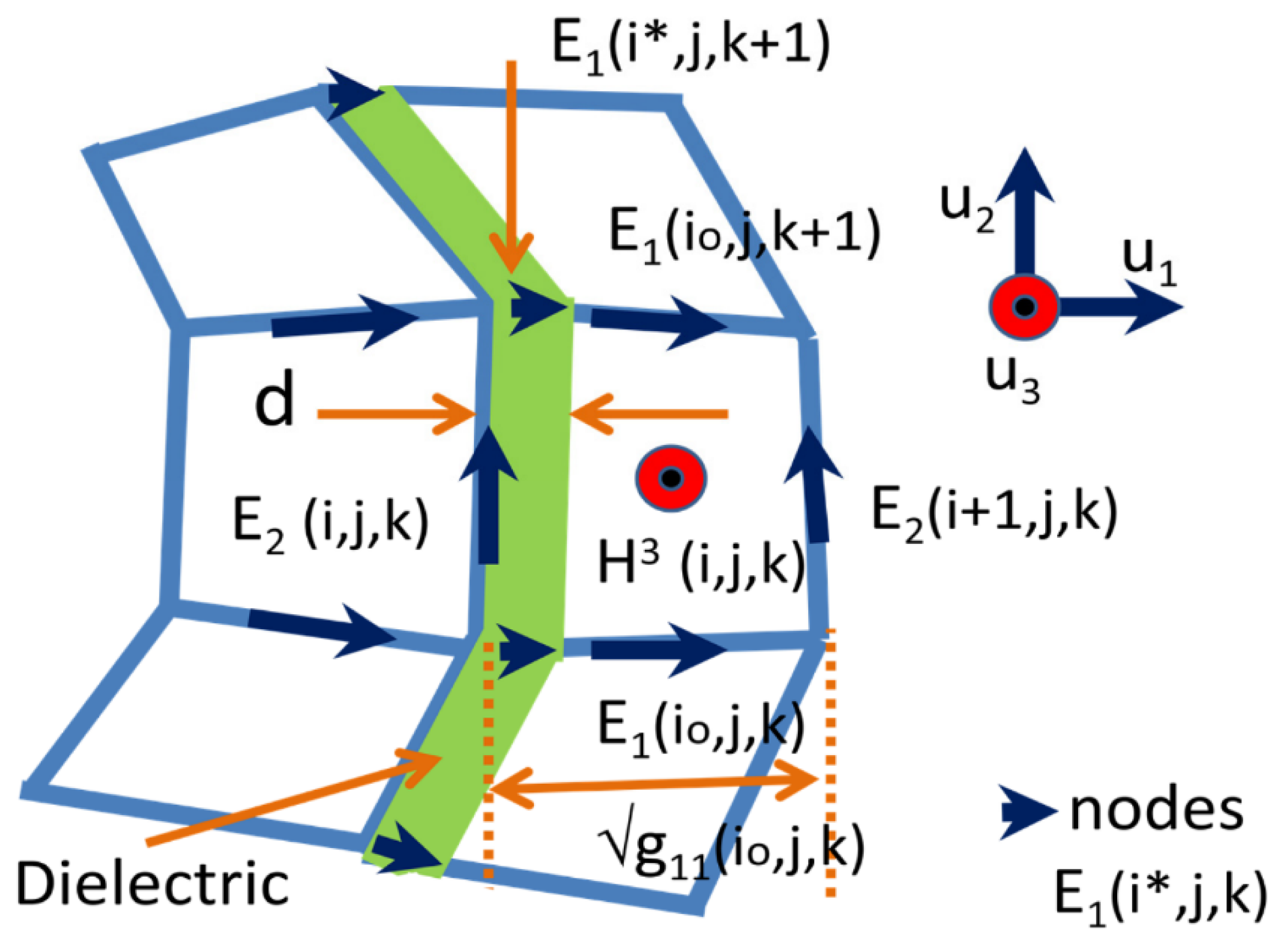
3. Sub-Cell Modeling of a Thin Dielectric Slab with Losses
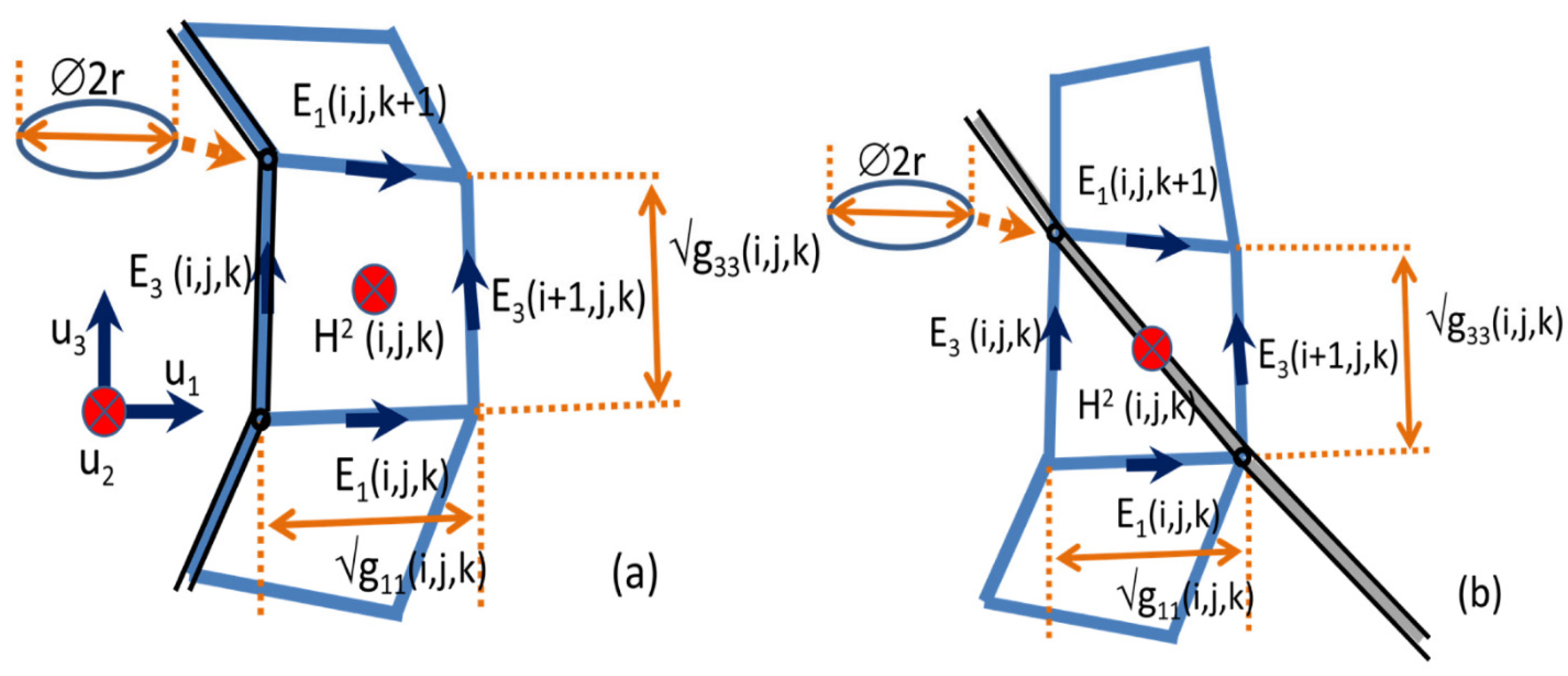
4. Thin Wire Sub-Cell Model
5. Finding the Optimal Radome Design for a Large Antenna array
5.1. Radome Design Strategy Using GA
- -
- Dielectric shell thickness, which will be chosen in the range 15–50 mm, for mechanical and manufacturing reasons.
- -
- Diameter of the silver metallic wire that will constitute the helix that envelops the radome.
- -
- Spacing between turns of the helical wire enveloping the radome.
- (1)
- Random production of an original population whose number of individuals is N.
- (2)
- Produce the next generation by crossovers and mutations among the individuals.
- (3)
- Produce the new population of N individuals from the generation of (2) by selection.
- (4)
- Produce the next population by repeating steps (2) and (3) until obtaining the individual that satisfies the optimal conditions defined.
5.2. FDTD-GA Optimization Scheme
- -
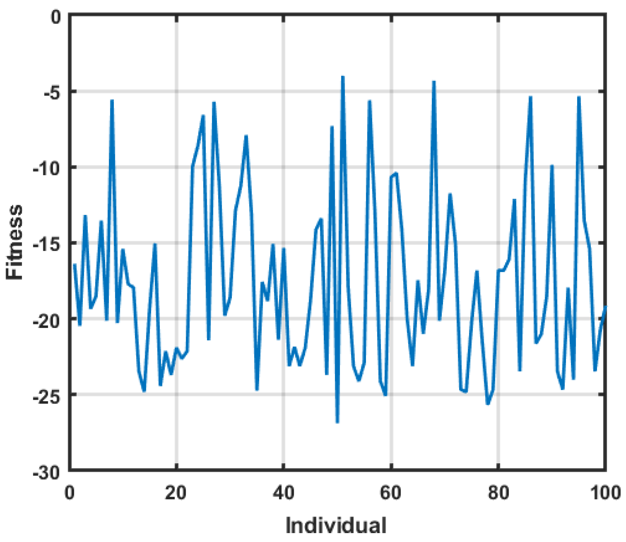
- Creation of a first population of n = 100 individuals
- ○
- n = 100 random binary 8-bit vectors are created as in Equation (28)
- ○
- Binary vectors are converted to decimal values in the given bounds, in this case (Thickness, diameter, spacing) ∈ [0.01, 0.05] × [0.10, 0.50] × [0.1 × 10−3, 1.0 × 10⁻³] in meters.
- ○
- Fitness is evaluated for each individual:
- ■
- Fitness is calculated by running FDTD for each individual (Thickness, diameter, spacing) in this population.
- -
- For i = 1: generation = G, do (searches optimum in G = 500 generations)
- ○
- Creation of a new population of 100 individual by crossing the individuals of the first population: Two offspring are born from a pair of two individuals, where the pair is randomly selected. There is randomly generated a point for bits (genes) In this way a new population is generated. A point of exchange of genes is randomly chosen to obtain the two offspring of the two parents.
- ○
- Mutation: A random number is generated, and if this number is greater than the given probability of mutation (pm ∈ [0.0, 1.0]), then bit 0 is changed to 1 and bit 1 is changed to zero, in the three randomly generated positions for each chromosome (Thickness, diameter, spacing) in binary.
- ○
- Calculation of fitness: F(S11) is calculated with FDTD for all the individuals of the population.
- ○
- Compares individuals in the population to find the one with the best fitness F(S11). This is compared against previous optimum value, and the best one between them is selected.
- ○
- Finds the individual with the worst fitness and this is substituted by the individual with the best fitness. With this process, the individuals with the worst fitness are eliminated from the population and replaced by those with the best fitness.
- -
- End
- -
- The best individual is obtained by comparison when fitness converges or by the end of generations.
6. Numerical Results
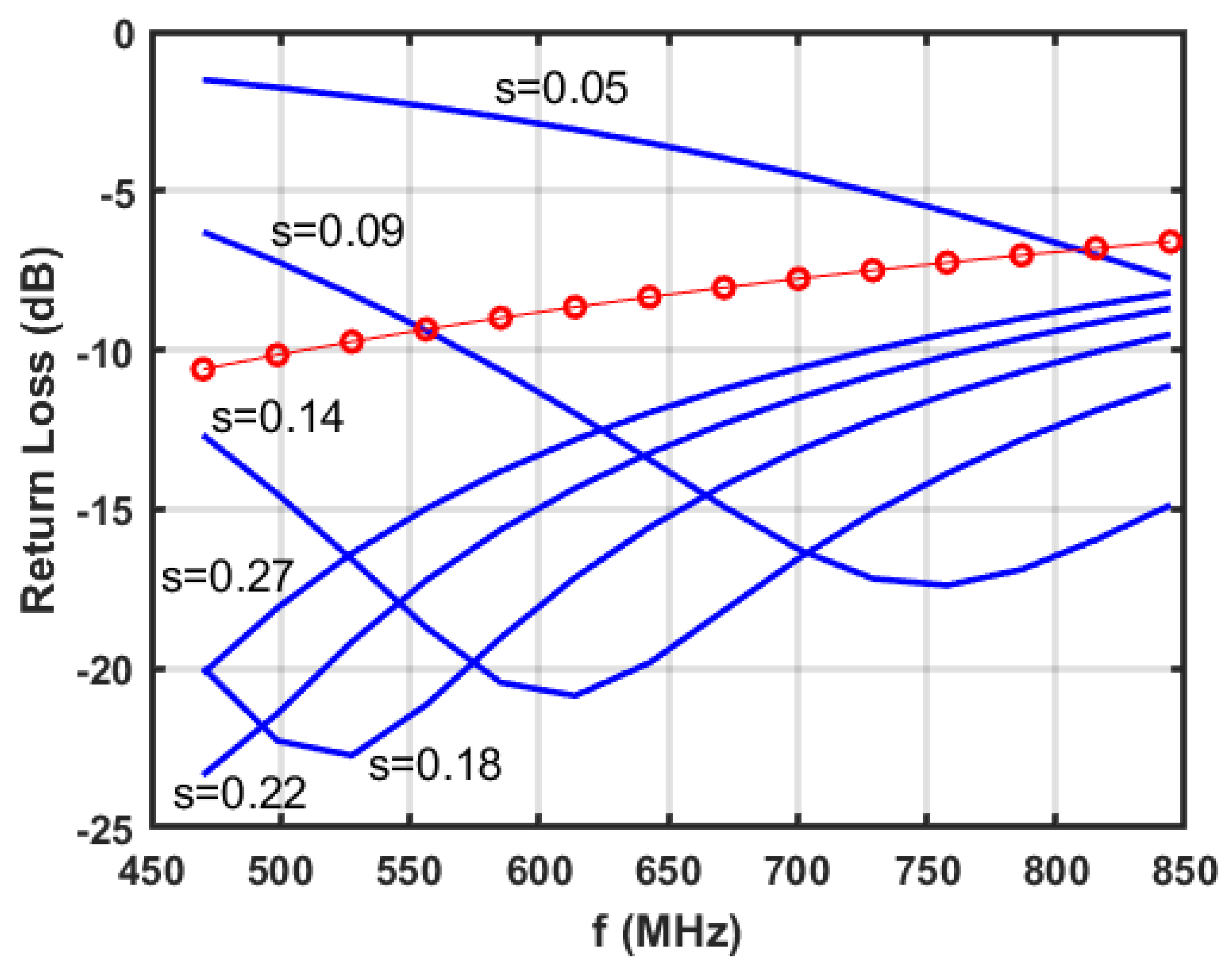
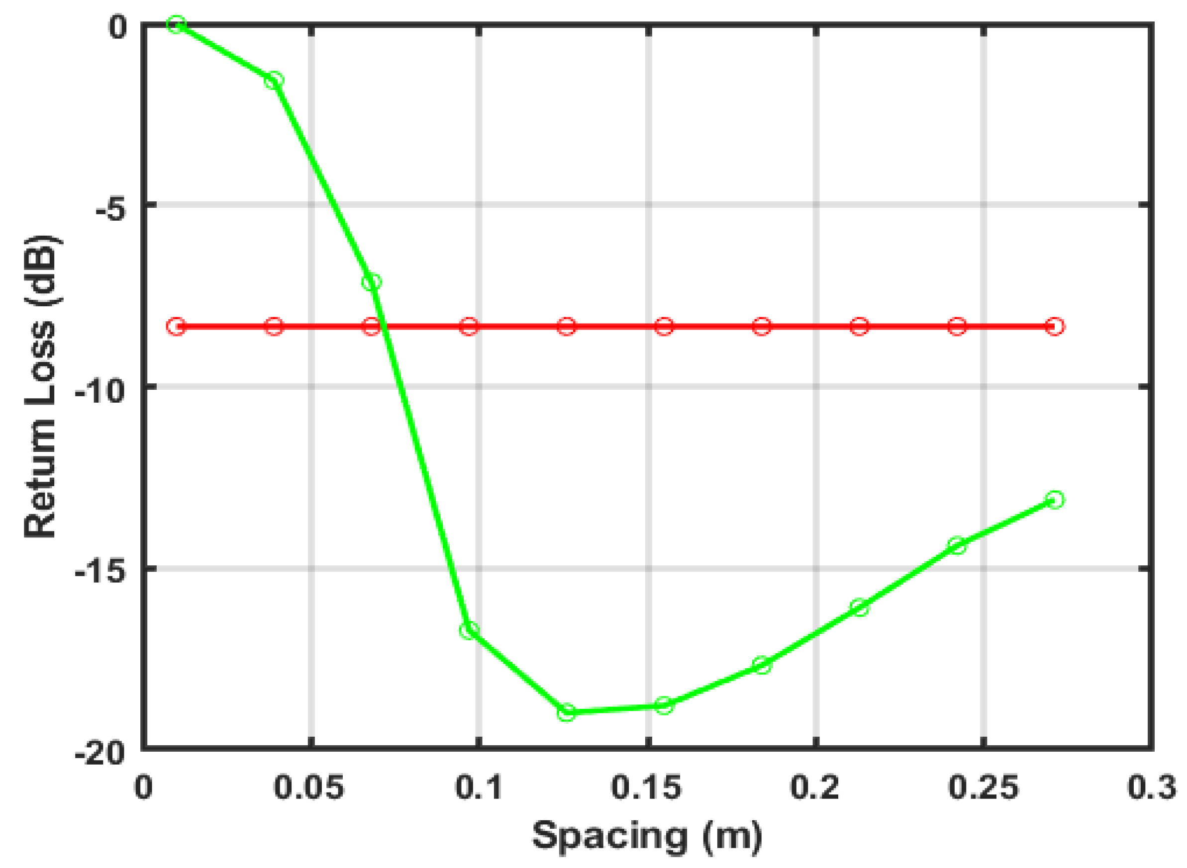
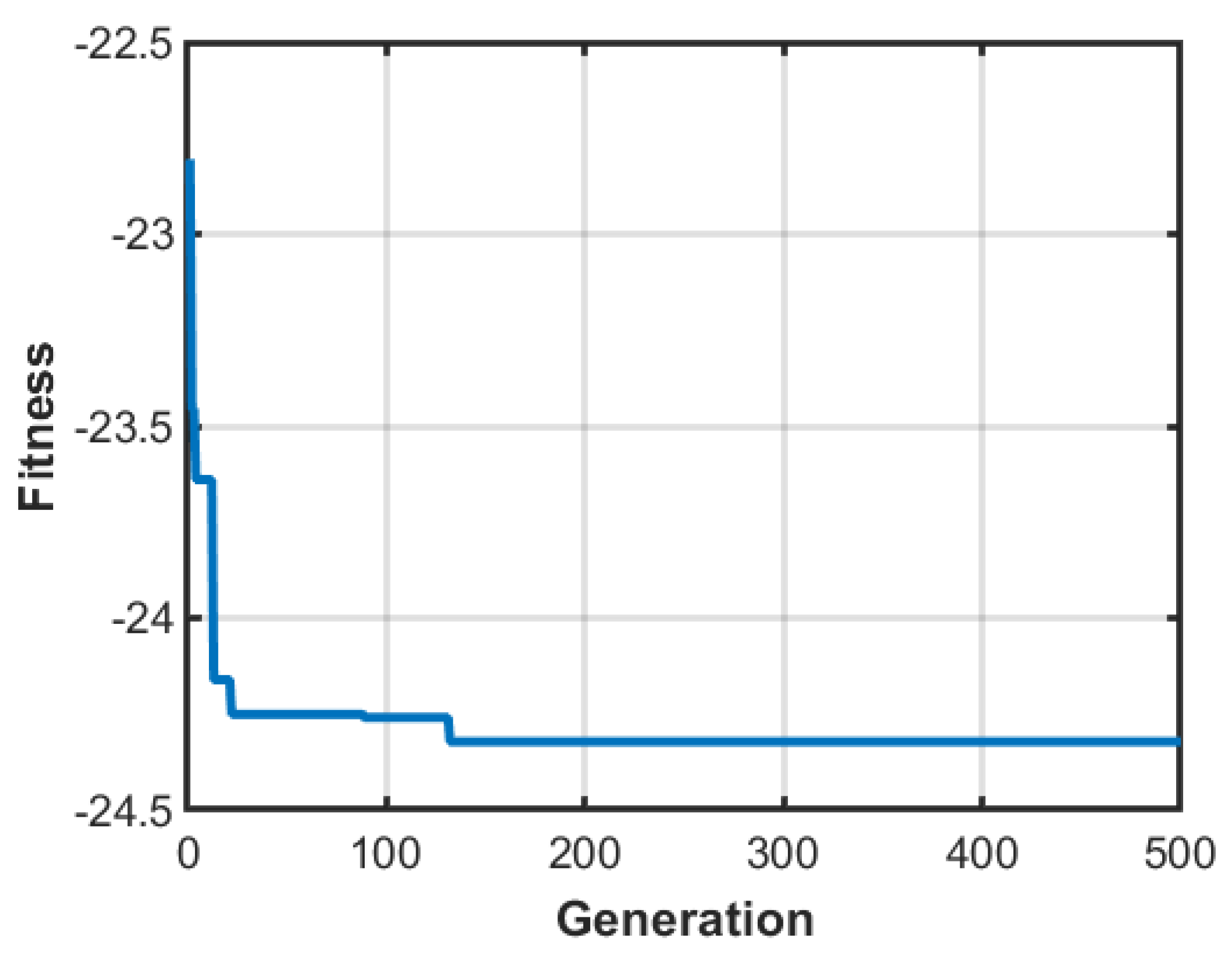
6.1. Return Loss
- -
- Thickness = 0.0100 m
- -
- Spacing = 0.1486 m
- -
- Wire diameter = 0.1 mm
- -
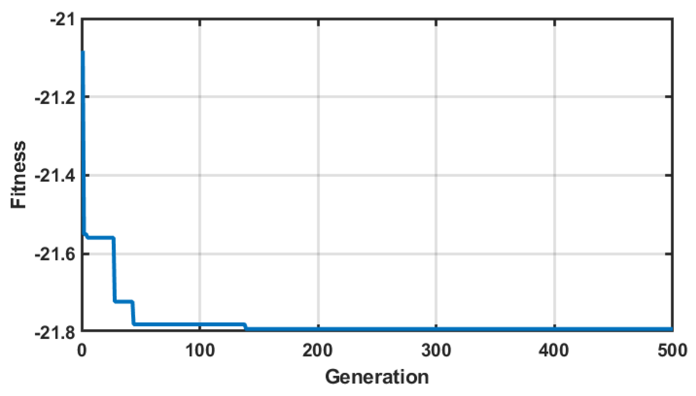
- Thickness = 0.0100 m
- -
- Spacing = 0.1565 m
- -
- Wire diameter = 0.1 mm
- -
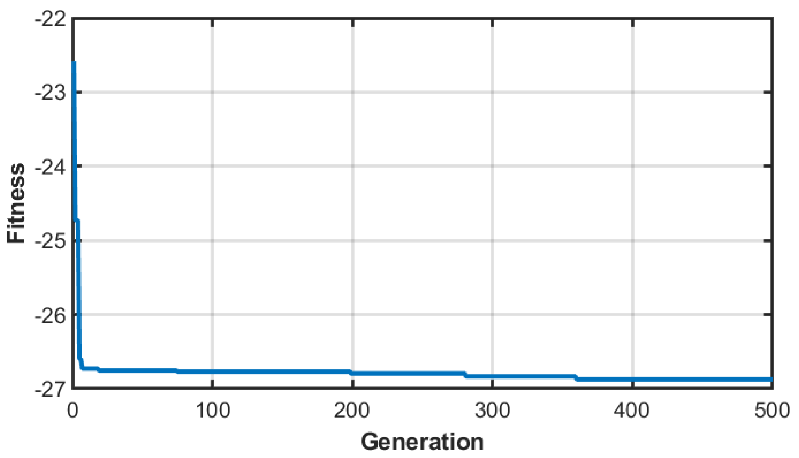
- Thickness = 0.0100 m
- -
- Spacing = 0.1502 m
- -
- Wire diameter = 0.1 mm
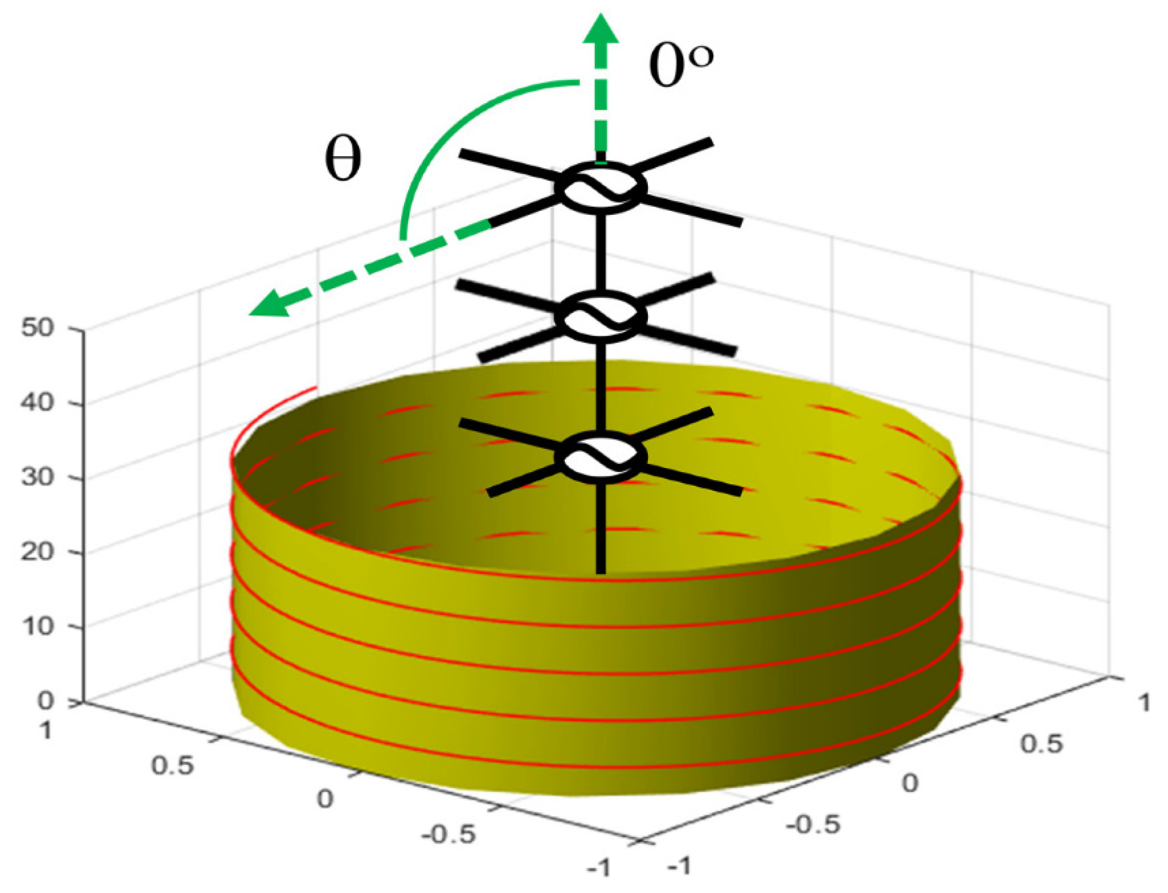
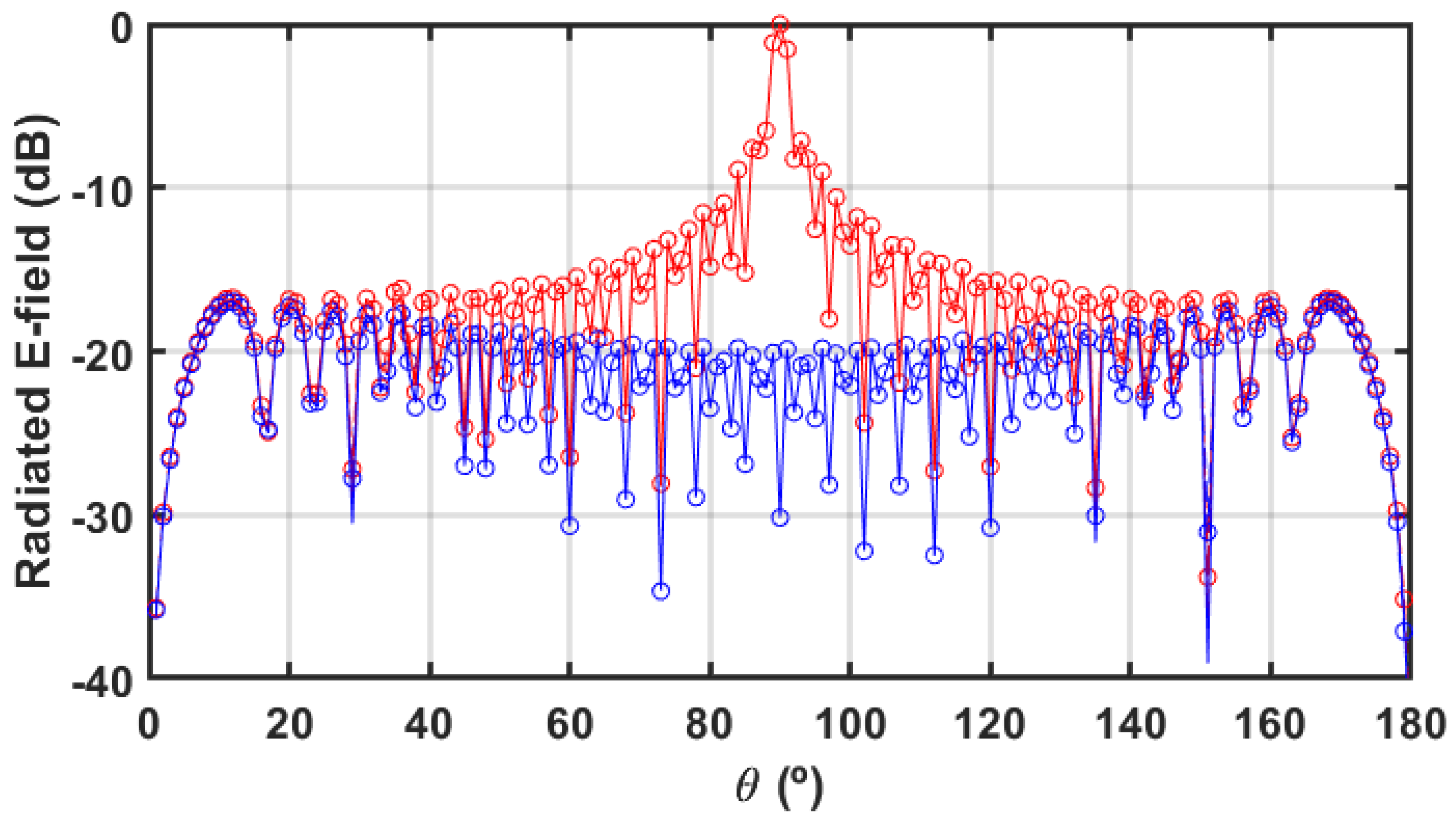
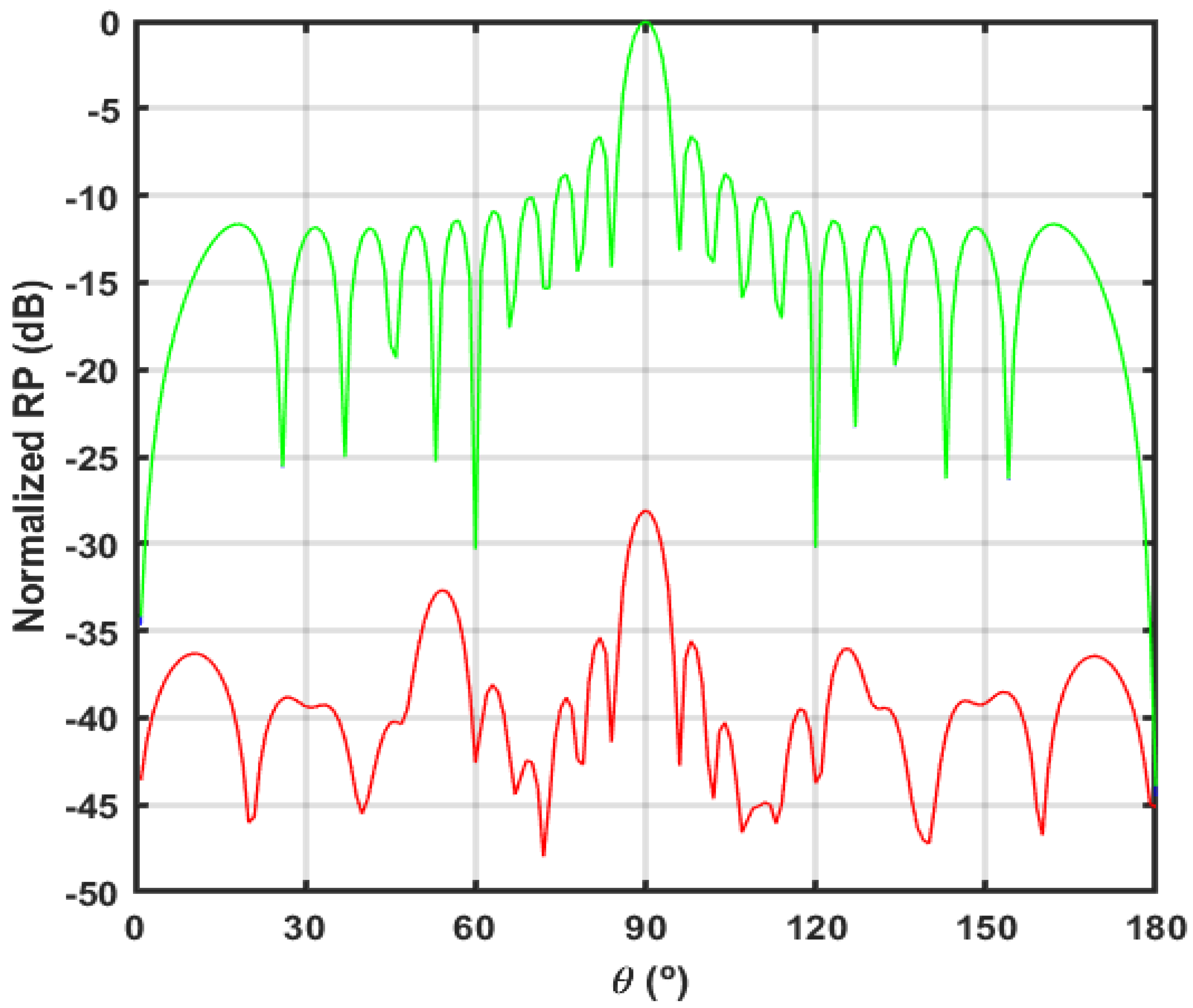
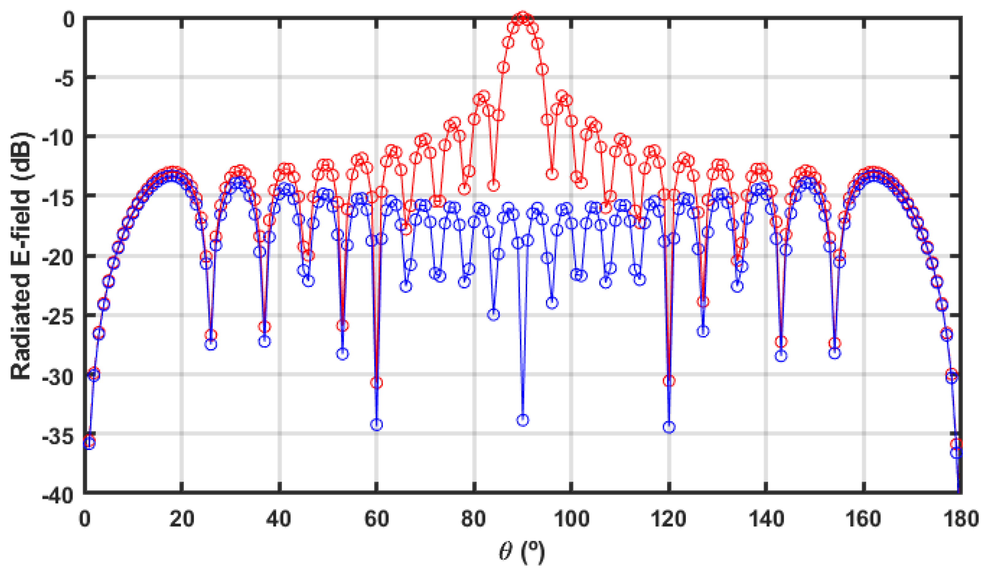
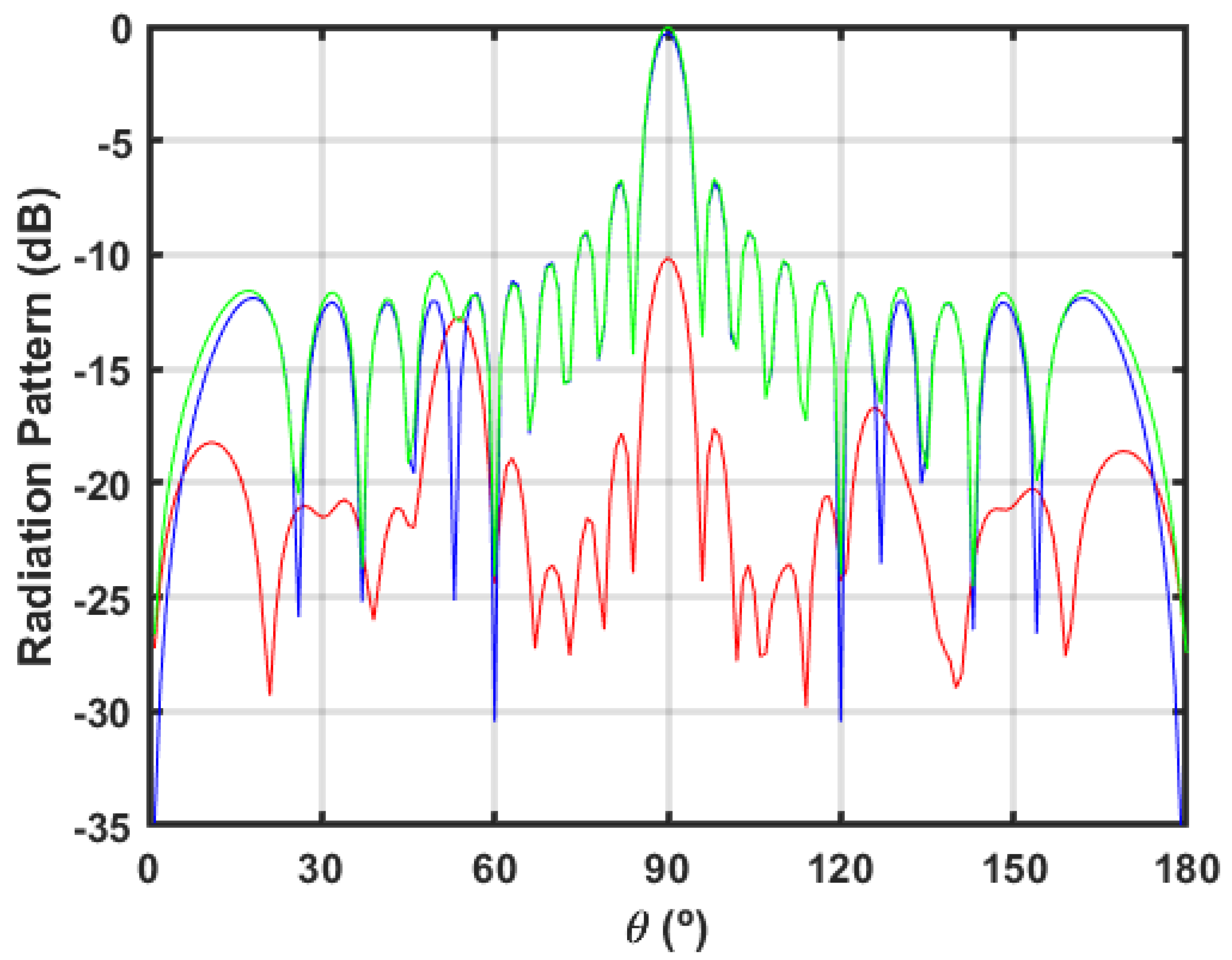
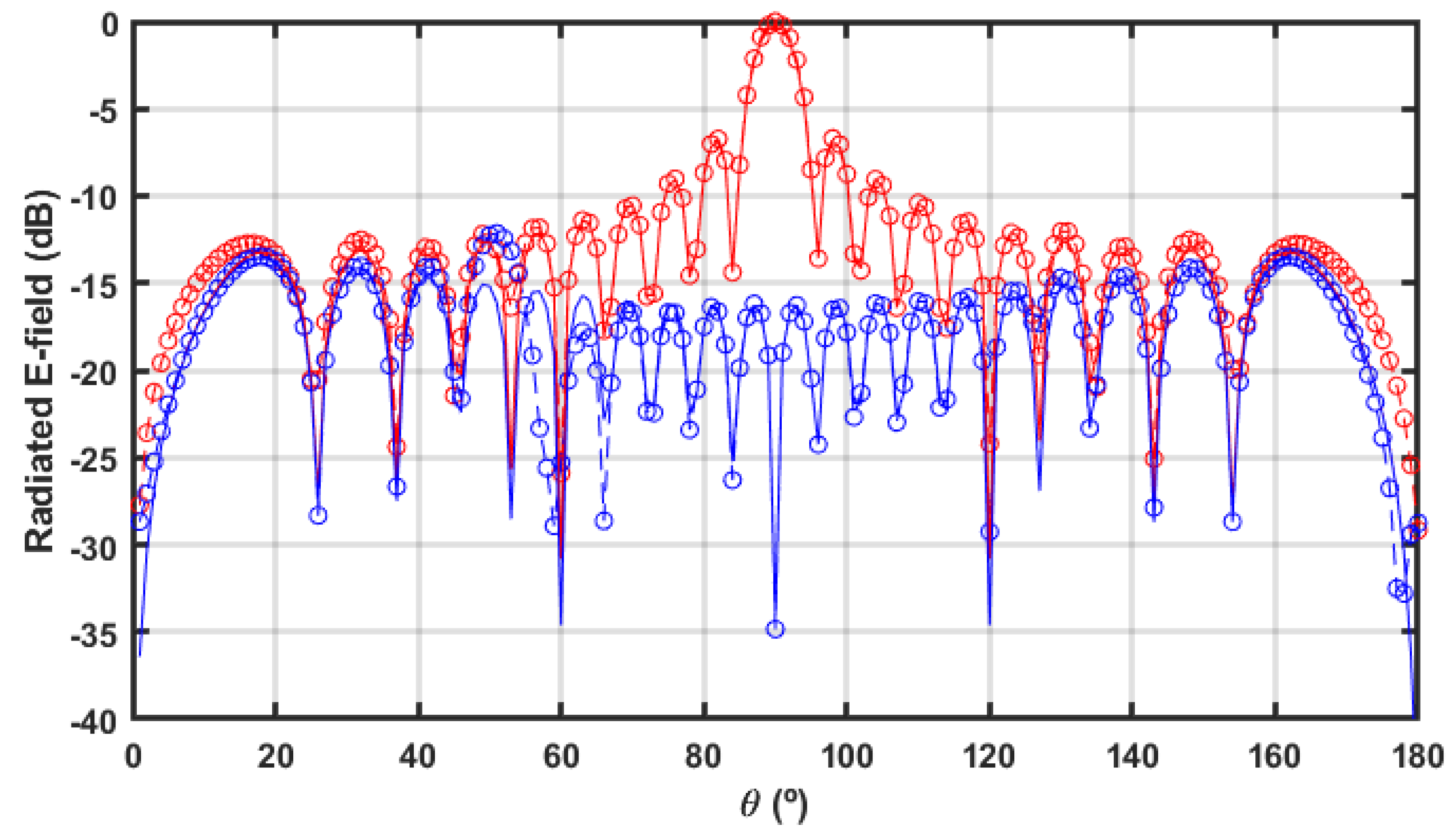
6.2. Radiation Pattern
7. Conclusions
Author Contributions
Funding
Acknowledgments
Conflicts of Interest
References
- Gimeno, B.; Such, V.; Garcia, A.C.; Cruz, J.L.; Navarro, E. Transmission-line model to analyze a multistage polarizer rotator. Microw. Opt. Technol. Lett. 1991, 4, 113–117. [Google Scholar] [CrossRef]
- Gimeno, B.; Cruz, J.; Navarro, E.; Such, V. Electromagnetic Scattering by a Strip Grating with Plane-Wave Three-Dimensional Oblique Incidence by Means of Decomposition into E-Type and H-Type Modes. J. Electromagn. Waves Appl. 1993, 7, 1201–1219. [Google Scholar] [CrossRef]
- Waqas, H.M.; Shi, D.; Imran, M.; Khan, S.Z.; Tong, L.; E Ahad, F.; Zaidi, A.A.; Iqbal, J.; Ahmed, W. Conceptual Design of Composite Sandwich Structure Submarine Radome. Materials 2019, 12, 1966. [Google Scholar] [CrossRef] [PubMed] [Green Version]
- Einziger, P.D.; Felsen, L. Ray analysis of two-dimensional radomes. IEEE Trans. Antenn. Propag. 1983, 31, 870–884. [Google Scholar] [CrossRef]
- Li, H.-Y.; Li, C.-M.; Gao, J.-G.; Sun, W.-F. Ameliorated Mechanical and Dielectric Properties of Heat-Resistant Radome Cyanate Composites. Molecules 2020, 25, 3117. [Google Scholar] [CrossRef]
- Friederich, F.; May, K.H.; Baccouche, B.; Matheis, C.; Bauer, M.; Jonuscheit, J.; Moor, M.; Denman, D.; Bramble, J.; Savage, N. Terahertz Radome Inspection. Photonics 2018, 5, 1. [Google Scholar] [CrossRef] [Green Version]
- Kim, J.; Lee, S.; Shin, H.; Jung, K.-Y.; Choo, H.; Park, Y.B. Radiation from a Cavity-Backed Circular Aperture Array Antenna Enclosed by an FSS Radome. Appl. Sci. 2018, 8, 234. [Google Scholar] [CrossRef] [Green Version]
- Rogers Corporation. High Frequency Circuit Material Data Sheets. Available online: http://www.rogerscorp.com/acs/literature.aspx (accessed on 5 August 2021).
- Duan, Z.; Abomakhleb, G.; Lu, G. Perforated Medium Applied in Frequency Selective Surfaces and Curved Antenna Radome. Appl. Sci. 2019, 9, 1081. [Google Scholar] [CrossRef] [Green Version]
- Hessel, A.; Sureau, J.-C. Resonances in circular arrays with dielectric sheet covers. IRE Trans. Antennas Propag. 1973, 21, 159–164. [Google Scholar] [CrossRef]
- Montgomery, J. Scattering by an infinite periodic array of thin conductors on a dielectric sheet. IRE Trans. Antennas Propag. 1975, 23, 70–75. [Google Scholar] [CrossRef]
- Pelton, E.; Munk, B. Scattering from periodic arrays of crossed dipoles. IRE Trans. Antennas Propag. 1979, 27, 323–330. [Google Scholar] [CrossRef]
- Cwik, T.; Mittra, R. Scattering from a periodic array of free-standing arbitrarily shaped perfectly conducting or resistive patches. IRE Trans. Antennas Propag. 1987, 35, 1226–1234. [Google Scholar] [CrossRef]
- Monni, S.; Gerini, G.; Neto, A.; Tijhuis, A.G. Multimode Equivalent Networks for the Design and Analysis of Frequency Selective Surfaces. IEEE Trans. Antennas Propag. 2007, 55, 2824–2835. [Google Scholar] [CrossRef] [Green Version]
- Paris, D.T. Computer Aided Radome Analysis. IEEE Trans. Antennas Propag. 1970, 18, 7–15. [Google Scholar] [CrossRef]
- Navarro, E.; Segura, J.; Soriano, A.; Such, V. Modeling of Thin Curved Sheets with the Curvilinear FDTD. IEEE Trans. Antennas Propag. 2004, 52, 342–346. [Google Scholar] [CrossRef]
- You, J.W.; Tan, S.R.; Zhou, X.Y.; Yu, W.M.; Cui, T.J. A New Method to Analyze Broadband Antenna-Radome Interactions in Time-Domain. IEEE Trans. Antennas Propag. 2013, 62, 334–344. [Google Scholar] [CrossRef]
- Shlager, K.L.; Schneider, J.B. A selective survey of the Finite-Difference Time-Domain Literature. IEEE Antennas Propag. Mag. 1995, 37, 39–56. [Google Scholar] [CrossRef] [Green Version]
- Navarro, E.; Gimena, B.; Cruz, J. Modelling of periodic structures using the finite difference time domain method combined with the Floquet theorem. Electron. Lett. 1993, 29, 446–447. [Google Scholar] [CrossRef]
- Navarro, E.; Bordallo, T.; Navasquillo-Miralles, J. FDTD characterization of evanescent modes-multimode analysis of waveguide discontinuities. IEEE Trans. Microw. Theory Tech. 2000, 48, 606–610. [Google Scholar] [CrossRef]
- Navarro, E.; Such, V.; Gimeno, B.; Cruz, J.L. T-junctions in square coaxial waveguide: A FD-TD approach. IEEE Trans. Microw. Theory Tech. 1994, 42, 347–350. [Google Scholar] [CrossRef]
- Navarro, E.A.; Such, V.; Gimeno, B.; Cruz, J.L. Analysis of H-plane waveguide discontinuities with an improved FD-TD algorithm. IEE Proc.-H 1992, 139, 183–185. [Google Scholar] [CrossRef]
- Reig, C.; Navarro, E.A.; Such, V. Full-wave FDTD design and analysis of wideband microstrip-to-waveguide transitions. Microw. Opt. Technol. Lett. 2003, 38, 317–320. [Google Scholar] [CrossRef]
- Navarro, E.; Sangary, N.; Wu, C.; Litva, J. Analysis of a coupled patch antenna with application in personal communications. IEE Proc. Microwaves Antennas Propag. 1995, 142, 495–497. [Google Scholar] [CrossRef]
- Reig, C.; Navarro, E.A.; Such, V. FDTD analysis of an E-sectoral horn excited by an opened microstrip. Microw. Opt. Technol. Lett. 1996, 13, 294–297. [Google Scholar] [CrossRef]
- Wu, C.; Navarro, E.A.; Navasquillo, J.; Litva, J. FDTD signal extrapolation using a finite impulse response neural network model. Microw. Opt. Technol. Lett. 1999, 21, 325–330. [Google Scholar] [CrossRef]
- Wu, C.; Navarro, A.; Litva, J. Combination of finite impulse response neural network technique with FDTD method for simulation of electromagnetic problems. Electron. Lett. 1996, 32, 1112–1113. [Google Scholar] [CrossRef]
- Navarro, E.; Gallart, L.; Cruz, J.; Gimeno, B.; Such, V. Accurate absorbing boundary conditions for the FDTD analysis of H-plane waveguide discontinuities. IEE Proc. Microwaves Antennas Propag. 1994, 141, 59–61. [Google Scholar] [CrossRef]
- Wu, C.; Navarro, E.A.; Chung, P.Y.; Litva, J. Modeling of waveguide structures using the nonorthogonal FDTD method with a PML absorbing boundary. Microw. Opt. Technol. Lett. 1995, 8, 226–228. [Google Scholar] [CrossRef]
- Maloney, J.; Smith, G. The use of surface impedance concepts in the finite-difference time-domain method. IEEE Trans. Antennas Propag. 1992, 40, 38–48. [Google Scholar] [CrossRef]
- Maloney, J.; Smith, G. The efficient modeling of thin material sheets in the finite-difference time-domain (FDTD) method. IEEE Trans. Antennas Propag. 1992, 40, 323–330. [Google Scholar] [CrossRef]
- Maloney, J.; Smith, G. A comparison of methods for modeling electrically thin dielectric and conducting sheets in the finite-difference time-domain (FDTD) method. IEEE Trans. Antennas Propag. 1993, 41, 690–694. [Google Scholar] [CrossRef]
- Stratton, J.A. Electromagnetic Theory; McGray Hill: New York, NY, USA, 1941. [Google Scholar]
- Holland, R. Finite-Difference Solution of Maxwell’s Equations in Generalized Nonorthogonal Coordinates. IEEE Trans. Nucl. Sci. 1983, 30, 4589–4591. [Google Scholar] [CrossRef]
- Ta, S.X.; Park, I.; Ziolkowski, R. Crossed Dipole Antennas: A review. IEEE Antennas Propag. Mag. 2015, 57, 107–122. [Google Scholar] [CrossRef]
- Calatayud, R.; Navarro-Modesto, E.; Navarro-Camba, E.A.; Sangary, N.T. Nvidia CUDA parallel processing of large FDTD meshes in a desktop computer: FDTD–Matlab on GPU. In Proceedings of the EATIS 2020, Aveiro, Portugal, 25–27 November 2020; pp. 3810–4193. [Google Scholar] [CrossRef]
- Weile, D.; Michielssen, E. Genetic algorithm optimization applied to electromagnetics: A review. IEEE Trans. Antennas Propag. 1997, 45, 343–353. [Google Scholar] [CrossRef]
- Elias, I.; Rubio, J.D.J.; Martinez, J.P.; Vargas, T.M.; Garcia, V.; Mujica-Vargas, D.; Meda-Campaña, J.A.; Pacheco, J.; Gutierrez, G.J.; Zacarias, A. Genetic Algorithm with Radial Basis Mapping Network for the Electricity Consumption Modeling. Appl. Sci. 2020, 10, 4239. [Google Scholar] [CrossRef]
- Park, K.M.; Shin, D.; Chi, S.D. Variable Chromosome Genetic Algorithm for Structure Learning in Neural Networks to Imitate Human Brain. Appl. Sci. 2019, 9, 3176. [Google Scholar] [CrossRef] [Green Version]
- Xin, J.; Zhong, J.; Yang, F.; Cui, Y.; Sheng, J. An Improved Genetic Algorithm for Path-Planning of Unmanned Surface Vehicle. Sensors 2019, 19, 2640. [Google Scholar] [CrossRef] [Green Version]
- Marcano, D.; Duran, F. Synthesis of antenna arrays using genetic algorithms. IEEE Antennas Propag. Mag. 2000, 42, 12–20. [Google Scholar] [CrossRef]
- Fornieles-Callejón, J.; Salinas, A.; Redondo, S.T.; Portí, J.; Méndez, A.; Navarro, E.A.; Morente-Molinera, J.A.; Soto-Aranaz, C.; Ortega-Cayuela, J.S. Extremely low frequency band station for natural electromagnetic noise measurement. Radio Sci. 2014, 50, 191–201. [Google Scholar] [CrossRef]
- Ansys HFSS. Broadband Adaptive Meshing. Available online: https://www.ansys.com/content/dam/product/electronics/hfss/ab-ansys-hfss-adaptive-broadband-meshing.pdf (accessed on 2 September 2021).
- Martinez, P.A.; Navarro, E.A.; Victoria, J.; Suarez, A.; Torres, J.; Alcarria, A.; Perez, J.; Amaro, A.; Menendez, A.; Soret, J. Design and Study of a Wide-Band Printed Circuit Board Near-Field Probe. Electronics 2021, 10, 2201. [Google Scholar] [CrossRef]
- Porti, J.; Morente, J.; Khalladi, M.; Gallego, A. Comparison of thin-wire models for TLM method. Electron. Lett. 1992, 28, 1910–1911. [Google Scholar] [CrossRef]
- Taniguchi, Y.; Baba, Y.; Nagaoka, N.; Ametani, A. An Improved Thin Wire Representation for FDTD Computations. IEEE Trans. Antennas Propag. 2008, 56, 3248–3252. [Google Scholar] [CrossRef]
- Asada, T.; Baba, Y.; Nagaoka, N.; Ametani, A. An Improved Thin Wire Representation for FDTD Transient Simulations. IEEE Trans. Electromagn. Compat. 2014, 57, 1–4. [Google Scholar] [CrossRef]
- Guiffaut, C.; Rouvrais, N.; Reineix, A.; Pecqueux, B. Insulated Oblique Thin Wire Formalism in the FDTD Method. IEEE Trans. Electromagn. Compat. 2017, 59, 1532–1540. [Google Scholar] [CrossRef]
- Liao, Z.P.; Wong, H.L.; Yang, B.P.; Yuan, Y.F. A transmitting boundary for transient wave analysis. Sci. Sin. Ser. A 1984, 27, 1063–1076. [Google Scholar]
- Navarro, E.; Litva, J.; Wu, C.; Chung, P. Application of PML superabsorbing boundary condition to non-orthogonal FDTD method. Electron. Lett. 1994, 30, 1654–1656. [Google Scholar] [CrossRef]
- Kraus, J. Helical Beam Antennas for Wide-Band Applications. Proc. IRE 1948, 36, 1236–1242. [Google Scholar] [CrossRef]
- Kraus, J.D. Antennas, 2nd ed.; McGraw Hill: New York, NY, USA, 1988; pp. 265–338. ISBN 0-07-035422-7. [Google Scholar]
- Sangary, N.T.; Nikolova, N.K. Line-of-sight approximation to the equivalence principle. IEEE Trans. Antennas Propag. 2004, 52, 1890–1897. [Google Scholar] [CrossRef]


| Fitness | Reflection | Thickness [0.01, 0.05] m | Spacing [0.10, 0.50] m | Wire Diameter [0.1, 1.0] mm |
|---|---|---|---|---|
| Equation (29) | −24.32 dB | 0.01 | 0.1486 | 0.1 |
| Equation (30) | −21.80 dB | 0.01 | 0.1565 | 0.1 |
| Equation (31) | −26.9 dB | 0.01 | 0.1502 | 0.1 |
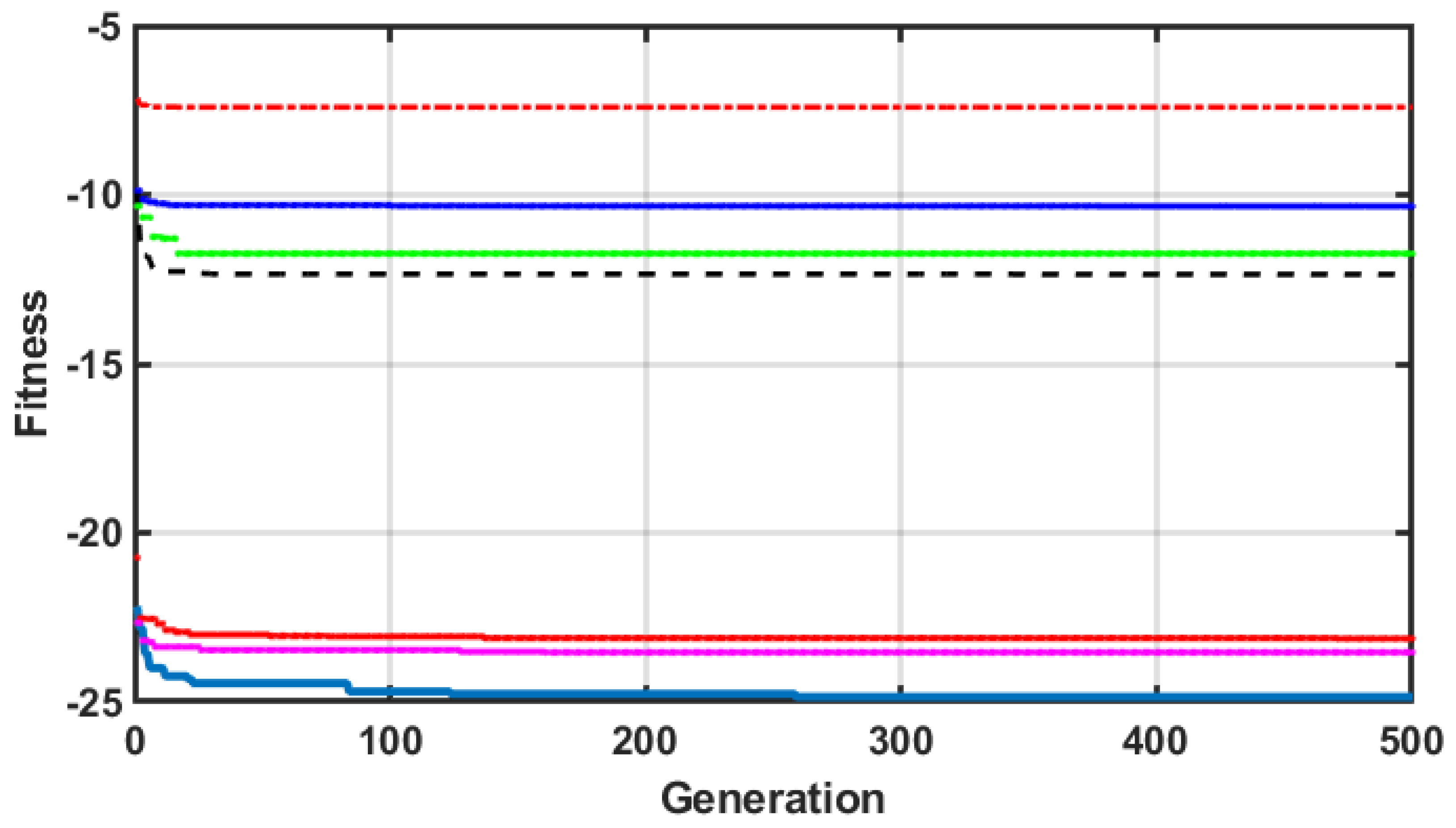
| Bounds GA-Thickness, Spacing, Wire Ø (m) | Reflection | Thickness (m) | Spacing (m) | Wire Ø (mm) |
|---|---|---|---|---|
| (1) [0.01, 0.05] × [0.10, 0.50] × [0.1 × 10−9, 1.0 × 10⁻³] | −24.9 dB | 0.01 | 0.12 | 0.02 |
| (2) [0.14, 0.20] × [0.005, 0.50] × [0.8 × 10−3, 2.0 × 10⁻³] | −7.4 dB | 0.14 | 0.11 | 1.0 |
| (3) [0.025, 0.05] × [0.01, 0.50] × [0.1 × 10−9, 1.0 × 10⁻³] | −12.35 dB | 0.025 | 0.06 | 0.02 |
| (4) [0.05, 0.10] × [0.005, 0.50] × [0.1 × 10−9, 1.0 × 10⁻³] | −11.74 dB | 0.100 | 0.29 | 1 × 10⁻⁷ |
| (5) [0.05, 0.10] × [0.005, 0.50] × [1.0 × 10−3, 3.0 × 10⁻³] | −10.34 dB | 0.100 | 0.50 | 1.00 |
| (6) [0.01, 0.10] × [0.005, 0.50] × [1.0 × 10−3, 3.0 × 10⁻³] | −23.13 dB | 0.100 | 0.21 | 1.00 |
| (7) [0.01, 0.10] × [0.005, 0.50] × [1.0 × 10−3, 3.0 × 10⁻³] | −23.54 dB | 0.008 | 0.25 | 1.00 |
Publisher’s Note: MDPI stays neutral with regard to jurisdictional claims in published maps and institutional affiliations. |
© 2021 by the authors. Licensee MDPI, Basel, Switzerland. This article is an open access article distributed under the terms and conditions of the Creative Commons Attribution (CC BY) license (https://creativecommons.org/licenses/by/4.0/).
Share and Cite
Navarro, E.A.; Portí, J.A.; Salinas, A.; Navarro-Modesto, E.; Toledo-Redondo, S.; Fornieles, J. Design & Optimization of Large Cylindrical Radomes with Subcell and Non-Orthogonal FDTD Meshes Combined with Genetic Algorithms. Electronics 2021, 10, 2263. https://doi.org/10.3390/electronics10182263
Navarro EA, Portí JA, Salinas A, Navarro-Modesto E, Toledo-Redondo S, Fornieles J. Design & Optimization of Large Cylindrical Radomes with Subcell and Non-Orthogonal FDTD Meshes Combined with Genetic Algorithms. Electronics. 2021; 10(18):2263. https://doi.org/10.3390/electronics10182263
Chicago/Turabian StyleNavarro, Enrique A., Jorge A. Portí, Alfonso Salinas, Enrique Navarro-Modesto, Sergio Toledo-Redondo, and Jesús Fornieles. 2021. "Design & Optimization of Large Cylindrical Radomes with Subcell and Non-Orthogonal FDTD Meshes Combined with Genetic Algorithms" Electronics 10, no. 18: 2263. https://doi.org/10.3390/electronics10182263