Developing a Realistic Simulation Environment for Robotics Harvesting Operations in a Vegetable Greenhouse

Abstract

Vegetable greenhouse operations are labour intensive. Automating some of these operations can save growers significant costs in an industry with low-profit margins. One of the most demanding operations is harvesting. Harvesting a tomato is a complex operation due to the significant clutter inherent to a greenhouse and the fragility of the object being grasped. Improving grasp and motion planning requires setting up a realistic testbed or testing on-site, which is expensive and time-limited to the growing season and specific environment. As such, it is important to develop a simulation environment to model this operation to help test various strategies before field testing can be conducted. Using the method presented in this work, 3D images are taken from a commercial greenhouse and used to develop a physics-based realistic simulation environment. The environment is then used to simulate a picking operation using various path planning algorithms to investigate the best algorithm to use in this case. The results show that this environment can be used to explore the best approaches to automate harvesting solutions in a vegetable greenhouse environment.

1. Introduction

Greenhouses are responsible for a significant amount of modern crop production worldwide. In Canada, the vegetable greenhouse industry was responsible for almost five hundred million kilograms of tomato harvest in 2020 alone [1], resulting in a farm gate value of $116 million. Historically in Canada, there has been a greenhouse labour shortage, as there were 2800 unfilled jobs in 2014, costing the horticultural industry approximately $100 million [2]. Automating the harvesting process can reduce labour cost and eliminate shortages. However, despite significant interest in the research community and funding agencies, a commercially viable harvesting robot for tomato greenhouses is not available. The problem has both technical and cost challenges making it difficult to have one system that can be deployed in different countries. Developing such a system is also expensive since testing various design iterations requires access to purposely built field facilities or commercial greenhouses during the growing season. We present one scenario where a robot is attempting to pick a tomato on a vine. Various path planning approaches can be tested and optimized before real-world testing. Within the Open Motion Planning Library (OMPL), there are many types of path planners available for testing. Some of the planners include randomized planners [3], potential-field planners [4], and search-based planners [5]. Some algorithms offer the ability to optimize trajectories with respect to smoothness [6], which is not offered with classical sampling-based approaches. Many of these planners are deviations from two very old planners, PRM [7], and RRT [8]. Many others, however, are standalone algorithms, such as KPIECE1 [9], PDST [10], and SBL [11]. Motion planning today is quite robust compared to what it was in the 1980s and 1990s, when planners were barely able to compute collision-free paths for objects translating and rotating in 2D workspaces [12].

To address this challenge, there have been several attempts to develop a robotics simulation environment for various agriculture projects, including greenhouses. The CROPS (Clever Robots for Crops) project [13] used a simulation in Gazebo to evaluate the robot without the requirement of taking the actual robot into the field. Nguyen et al. developed a framework of the motion planning task for the CROPS robot [14]. He used an apple tree simulation environment with only the tree trunk and branches considered as obstacles. Shamshiri et al. [15] provide a review of various simulation software that can be used for developing simulation environments for agriculture applications. Shamshiri et al. [16] created a simulated environment that could be used for the harvesting of vegetables. A replica of the different manipulators, sensors, and a sweet pepper plant was included in this simulation. In all of the previous efforts, artificial models of plants were used in the simulation.

While these models can be adequate for some operations, in this paper, we attempt to bridge the gap between the real-world environment and the simulation environment by including data obtained from 3D images of a commercial greenhouse. This approach has been proposed for mobile robotics applications [17] but not for greenhouse environments. Data acquired from an operational greenhouse environment will be processed and imported into a robotics simulator and tuned to enable testing of various harvesting operations. We present one scenario where a robot is attempting to pick a tomato on a vine. Various path planning approaches can be tested and optimized before real-world testing. Furthermore, this integration between the physical and simulation environment can be continuous, enabling testing of the harvesting operation during the entire growth season with various levels of clutter and occlusion. The data can also be used for the prediction of yield and optimizing greenhouse operations. The contributions of this paper are:

• Present a method to create a realistic simulation of vegetable greenhouse environments that include various obstacles and clutter. The method integrates real-world data into a physics-based robotics simulation software.
• Demonstrate how to use this environment to test robotics harvesting operations.

2. Materials and Methods

2.1. Robotics Simulation Platform

There are multiple different simulators and virtual environments that can be used for testing designs. Each simulator has its own set of merits and limitations, which may cause one type of simulator to be more suited to a specific task than the others. A comparative paper that addresses this issue can be seen in [15], where simulators VREP, Gazebo, and ARGoS are compared against each other based on their respective performances within similar scenes. Small and large scenes were compared with a changing number of robots. Of the three simulations, VREP achieved the slowest simulation speed and the highest memory usage. ARGoS had the fastest simulation speed for small scenes, but was taken over by Gazebo as the scene size increased. However, despite V-REP’s lacking simulation speed, carefully setting simulation parameters and optimizing 3D models can drastically increase its performance. This is also shown in [18], where a feature comparison is done between the V-REP, Gazebo, and ARGoS simulators. With respect to the features available in the simulators, V-REP has the largest collection of features such as a scene editor, 3D model importing, and mesh manipulation. A significant disadvantage of V-REP is its inability to define a scene in an XML file. This would allow multiple experiments with varying parameter values to be run automatically. While V-REP is the most complex of the three simulators, it offers many features which are not available otherwise.

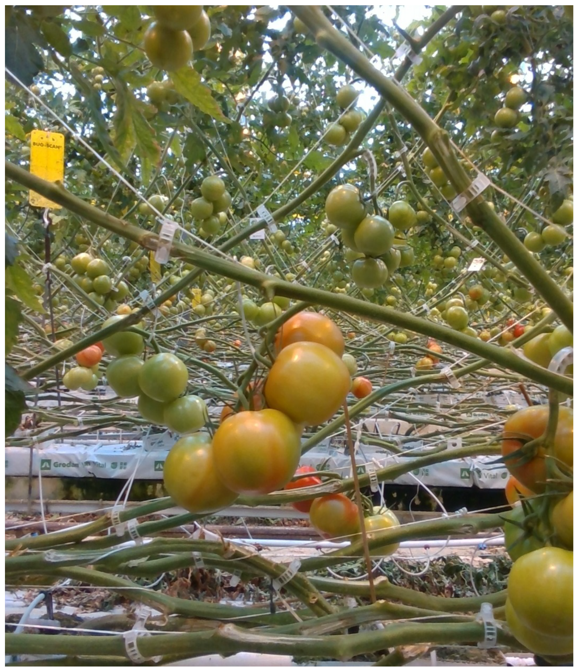
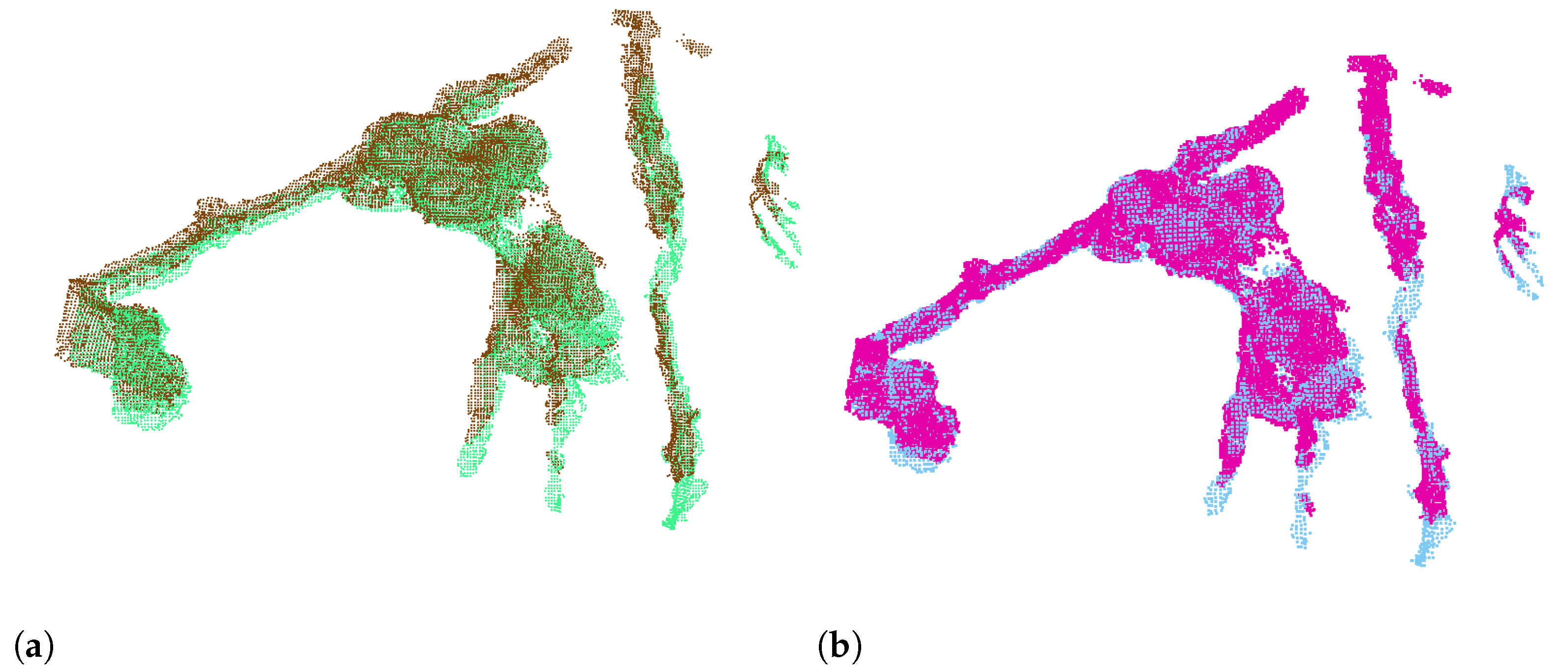
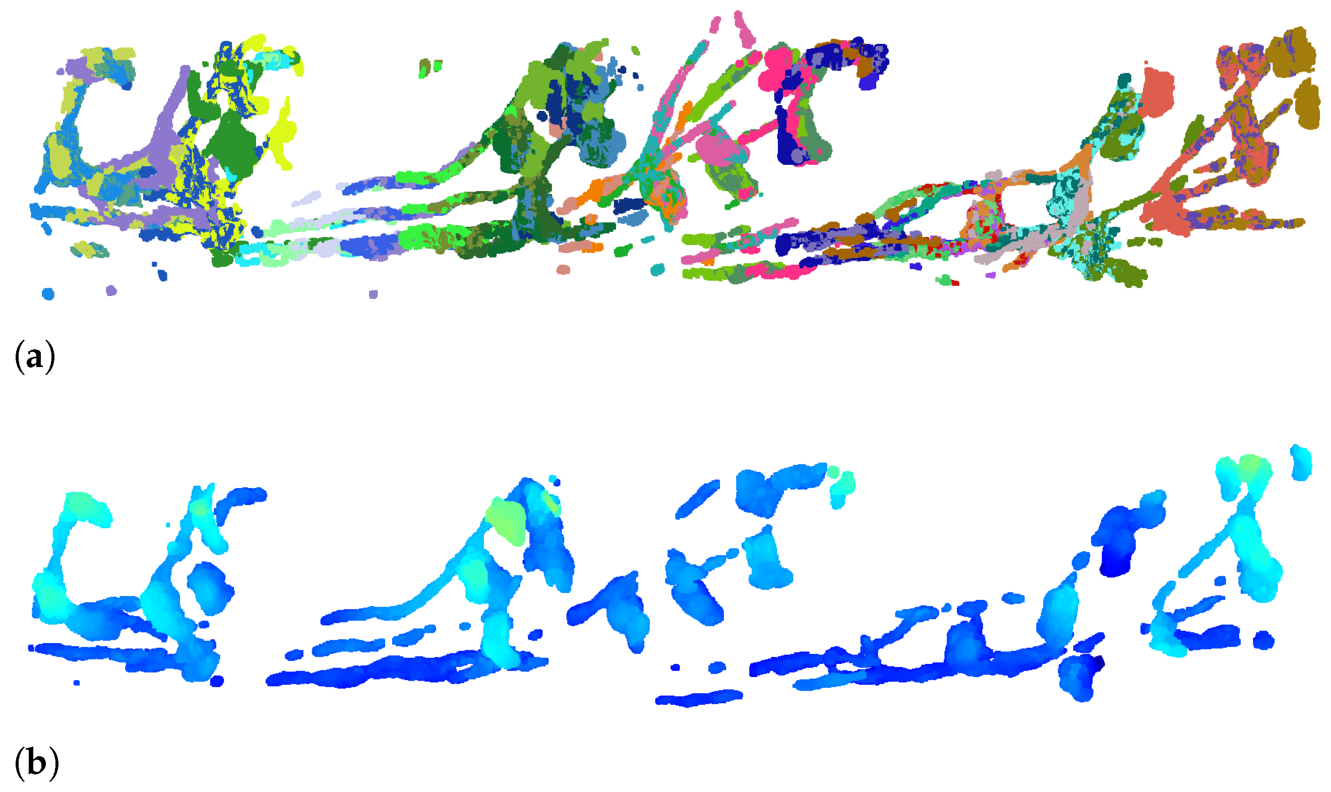
2.2. Three-Dimensional Mapping of a Vegetable Greenhouse

Figure 1 provides a brief overview of the methodology discussed in this section, as well as the Simulation Environment section.

In order to adequately create a simulation that mimics a greenhouse environment, the environment should reflect actual data from a greenhouse. Figure 2 shows an image taken from a commercial tomato greenhouse in Ontario, Canada. This represents a sample of the environment we wish to mimic in the simulation environment.

To enable simulation of a robotic picking operations, it is important to have a 3D map of the environment. To accomplish this task, images were collected using a three-camera system mounted on a tripod placed approximately 50 cm along the normal to each plant. Images were taken of the plant side along each row. The tripod was manually moved along the greenhouse rows, and images were collected approximately every 10 cm. An example of the collected images is seen in Figure 2. This process was repeated for two greenhouse rows. For each row, 150 images were captured for a total of 300 images. These images represent part of each row covering only the first 60 plants/row.

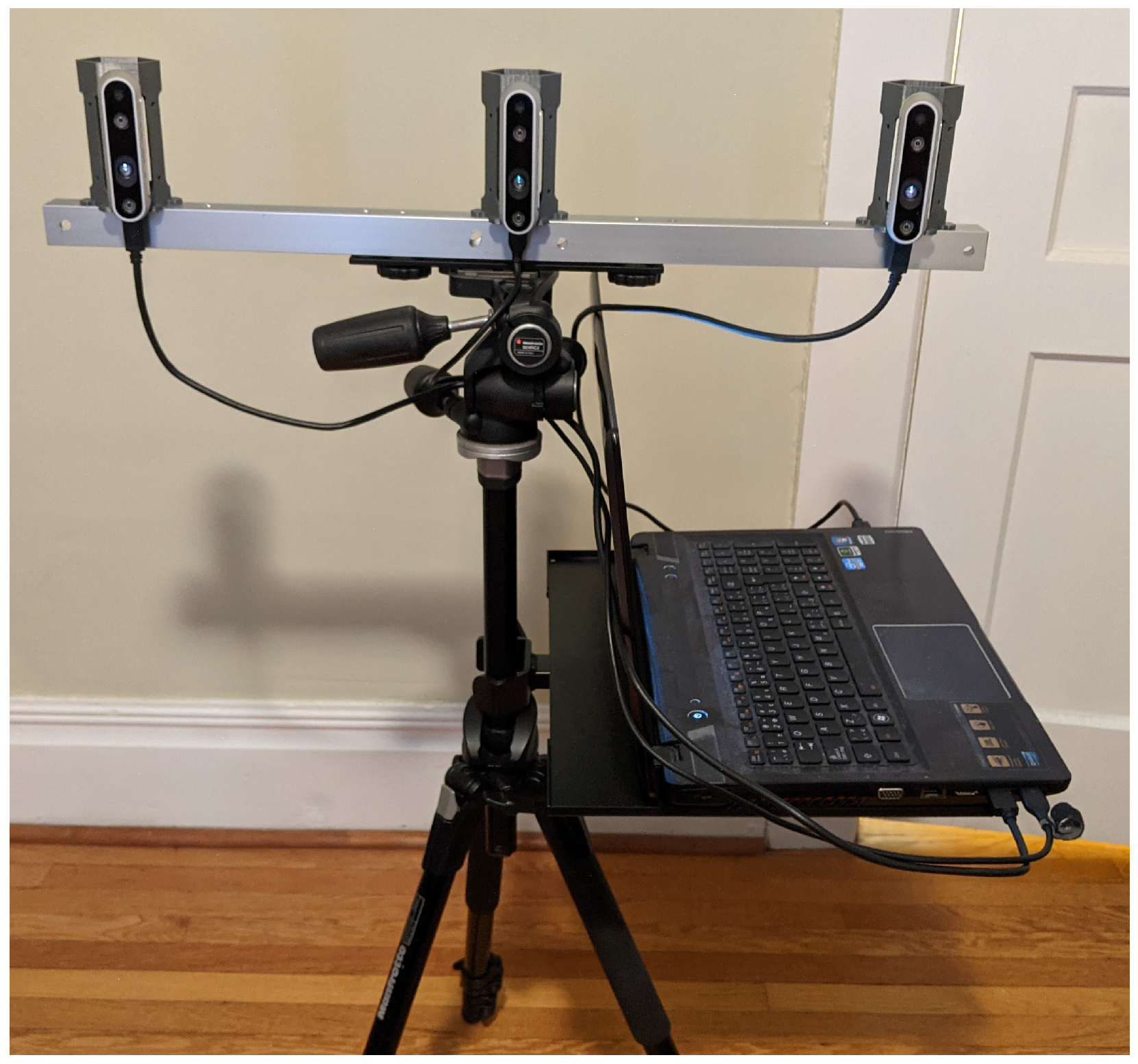
2.2.1. RGB-D Image Capture System

The RGB-D image capture system included three Intel® RealSense™ D435 cameras (Intel, Santa Clara, CA, USA) mounted on a tripod along with a laptop for collecting and storing the images. This camera has a colour camera sensor and two infrared sensors. The latter was used to detect the depth using stereo vision. The cameras were placed on a metal beam 25 cm apart, as shown in Figure 3. The outer two cameras were angled 25° toward the centre in order to obtain a more complete 3D view of the plants.

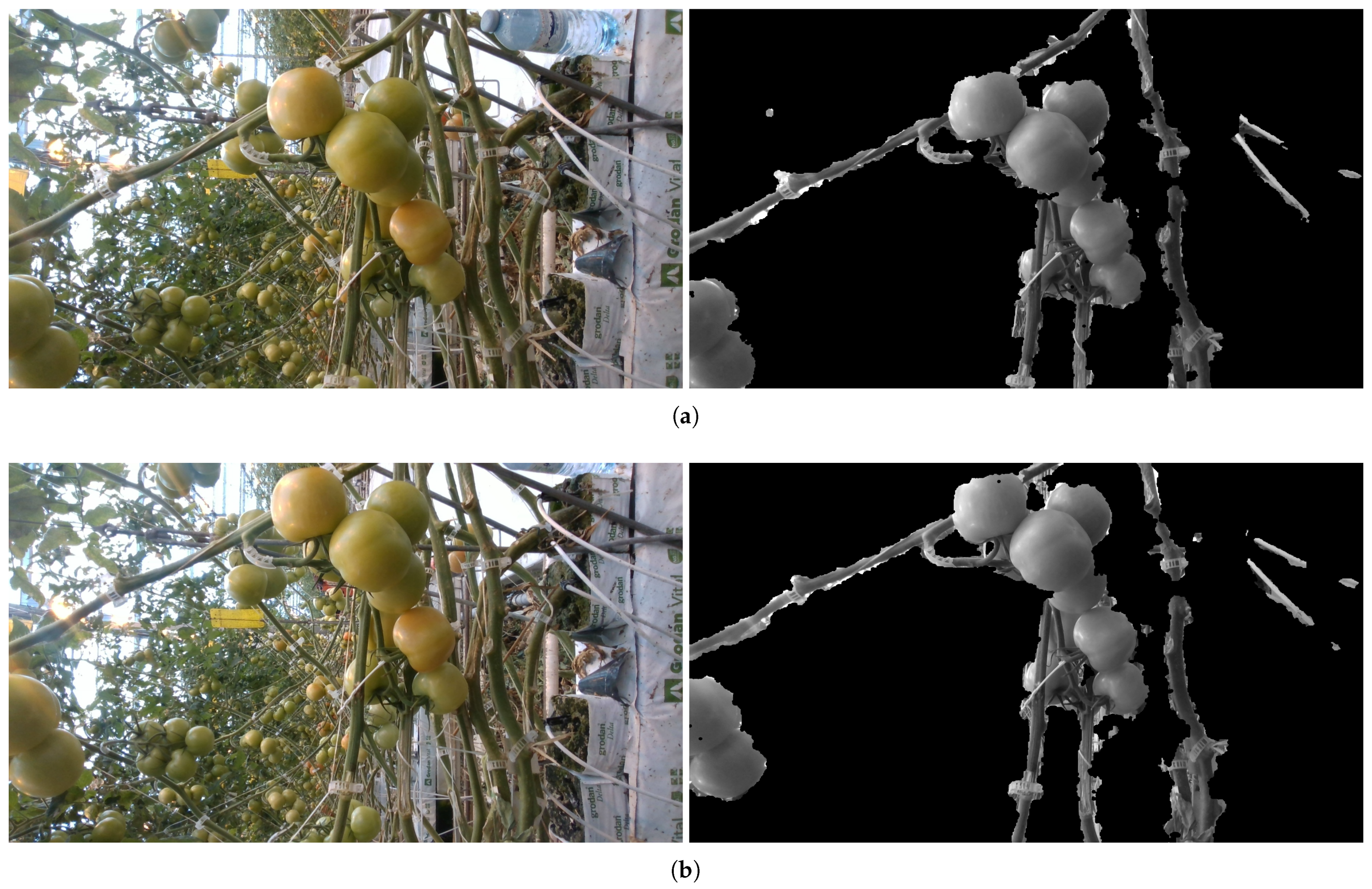
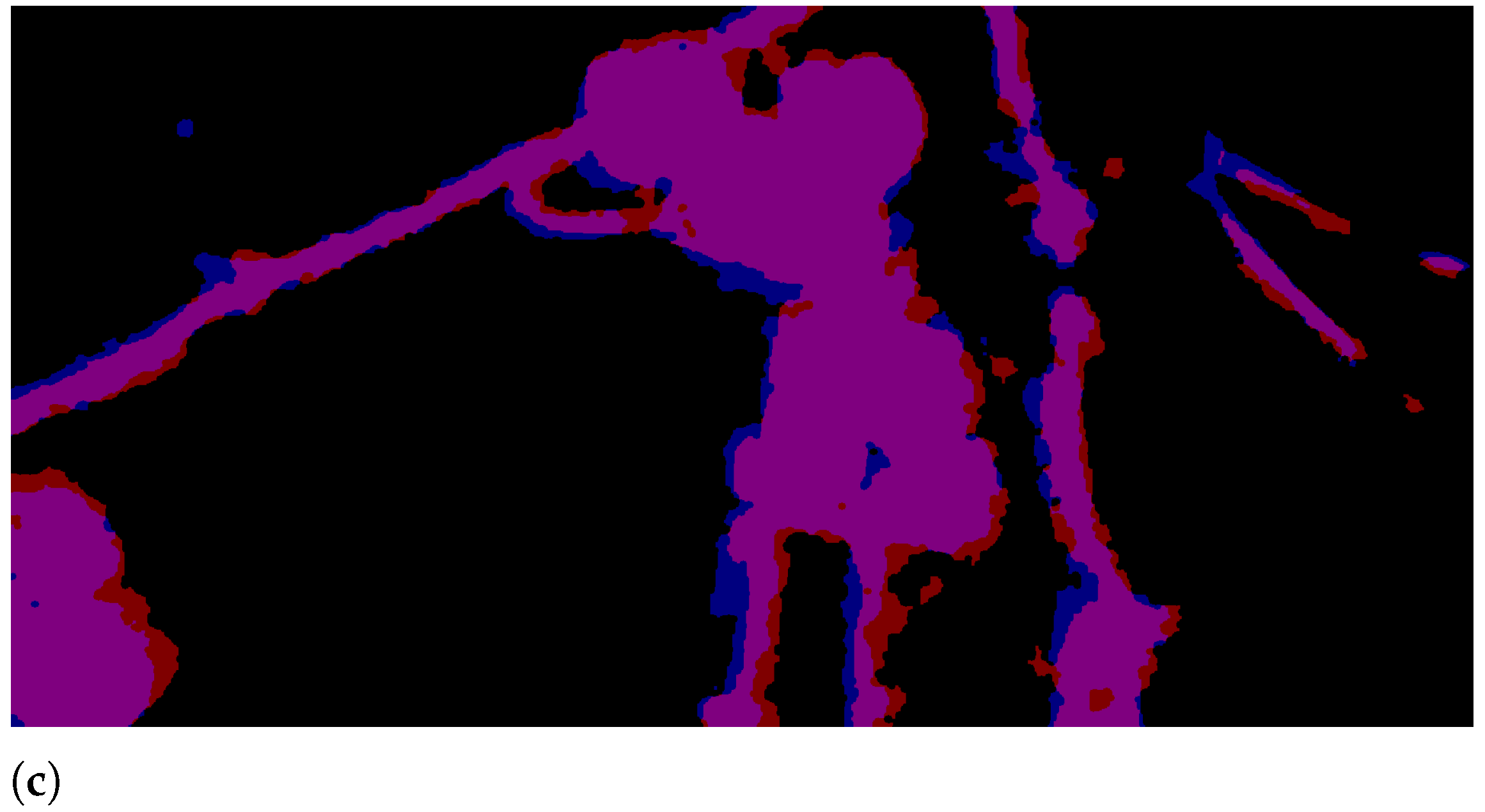
2.2.2. RGB-D Image Processing

The image processing algorithm was developed using Python and the open source OpenCV [19] and Open3D [20] libraries. The purpose of the algorithm is to combine the 3D data from the Realsense cameras to generate individual point clouds. Then all the point clouds from successive images are combined in order to generate a combined 3D point cloud of the entire row of plants.

The first step is to combine the 3D data from the different cameras into a single coordinate frame. Due to technical issues, we were not able to utilize the data from the camera on the right, and therefore only combined the data from the centre and left cameras. We chose the centre camera as the origin, and transformed the data from the left camera into this coordinate frame. As the cameras are at a fixed angle and distance relative to one another, this was possible using a constant transformation matrix.

Once the data from multiple cameras were combined, the next step was to stitch the successive images obtained as the cameras were moving along the row to create a continuous image of the greenhouse row. The RGB processing was performed using the images from the centre camera as it stays parallel to the row as the tripod moves. The process starts with removing the background plants by identifying regions in the depth image that are more than 60 cm from the camera. This background removal allows us to focus on the nearest vines and tomatoes. A sample of two successive images with the background removed is shown in Figure 4.

Next, we shift one of the images to attempt to match the foreground with the other image. The match is based only on the general shape of the foreground by setting the entire foreground white and the background black. Next, we gradually shift the first image up a few pixels at a time and subtract the images from one another until we find the pixel difference that produces the least difference between the images. An example of the comparison after shifting the first image is shown in Figure 5, where the blue and red images combine to show the shared purple regions between the images. This is the point at which the minimum pixel difference is achieved.

Once the shared regions in the successive images have been identified, we further refine the process using additional 3D data. For each image, we examine all of the shared pixels we identified from the RGB and determine their depth values using the aligned depth image. Using the depth value and the camera intrinsics, we can determine the XYZ position of each pixel relative to the camera coordinate frame. Using the shared pixels in successive images, we can determine the XYZ distance each pixel has moved since the last image and, therefore, determine the distance the camera has moved. While we know the tripod was manually moved approximately 10 cm along the row for each image, this provides us with a more accurate distance of the camera movement.

Once the camera movement is known, we can shift the 3D point clouds so that they are roughly aligned. As there may have also been some small changes in the angle of the cameras or distance from the plants, we can further refine the registration of the successive point clouds using iterative closest point (ICP). ICP is used here to minimize the distance between points in two point clouds. More information regarding ICP can be found in [21]. We use ICP implemented in the Python Open3D library to do so. An image of the two point clouds before and after using ICP is shown in Figure 6.

The RGB and 3D processing stages are repeated for all the available images to create a complete 3D point cloud of the row. In some cases, the RGB or 3D processing may fail to properly register two successive images together. In this case, the second image is skipped over, and we attempt to register the third image with the first image in the succession.

Once all of the successive images of the greenhouse row have been combined, some postprocessing is performed to simplify the point cloud. We use the radius outlier removal function in Open3D [20] to remove points that have less than 200 neighbours in a 5 cm radius. This removes any points that do not have a high degree of overlap as they may have failed to properly register in the RGB processing and ICP stages. A sample point cloud using 50 successive images before and after the outlier removal is shown in Figure 7.

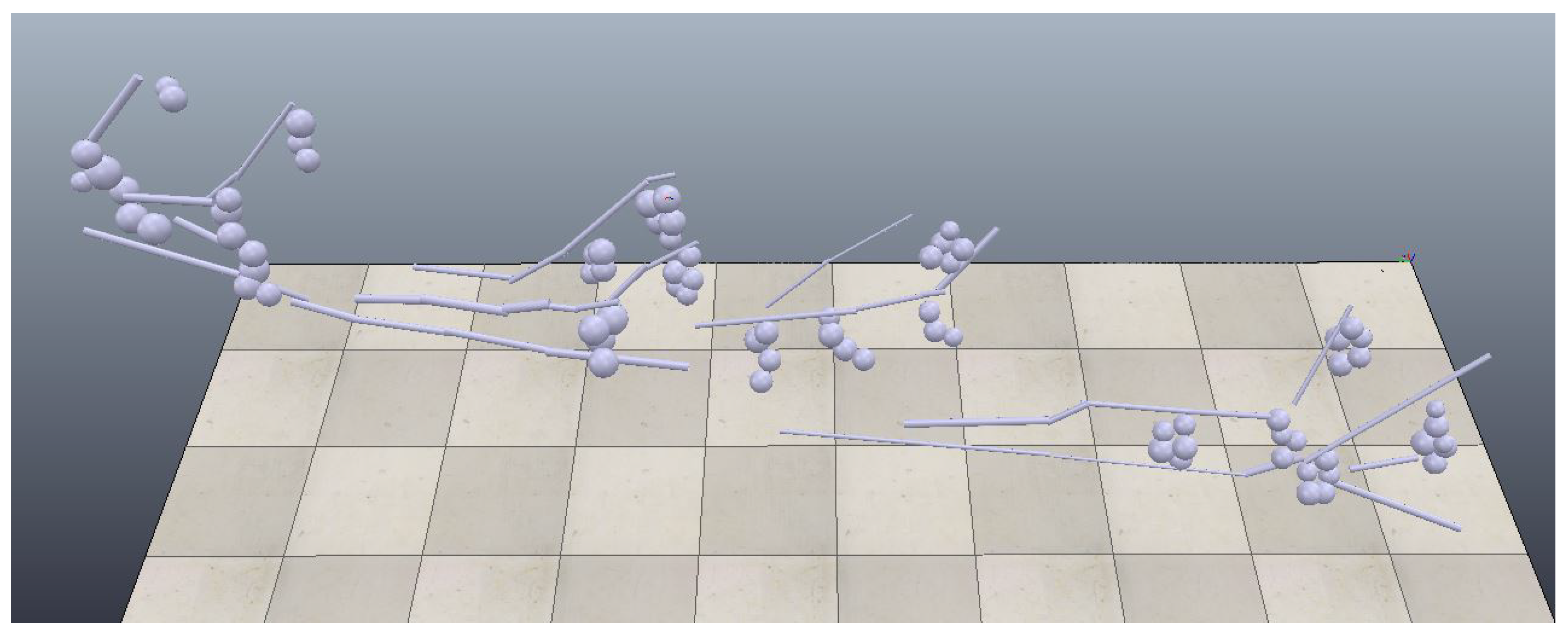
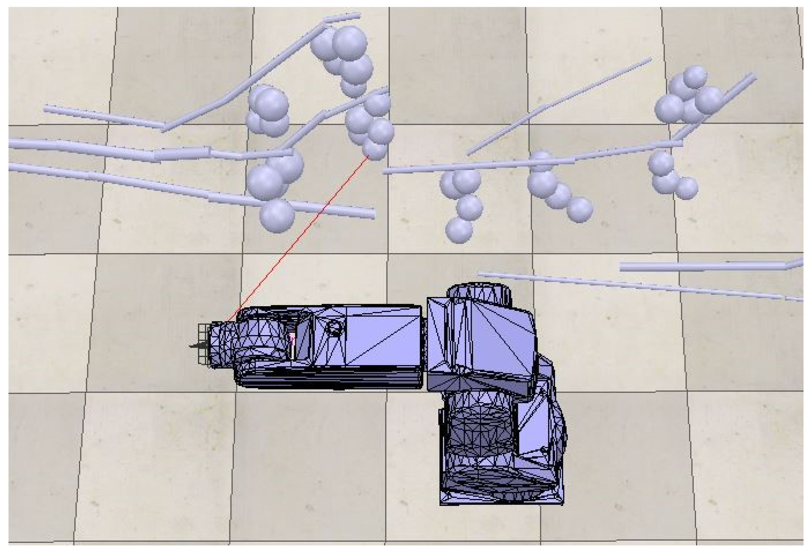
2.3. Simulation Environment

To import the point cloud into the robotics simulation environment, they are first converted into a triangular mesh. The mesh is then imported into CoppeliaSim [22] where it was then decomposed into cylinders and spheres, representing branches and tomatoes. The positions of the branches and tomatoes were determined using the remainder of the pointcloud image shown in Figure 7.

The point cloud was originally composed of 295,490 points by default; at this density it was computationally taxing to convert the point cloud into a triangular mesh. Meshlab [23] was used to complete the transition from point cloud to triangular mesh. It takes over an hour to convert the point cloud into a mesh. Beyond the processing time, it was effectively impossible to use within CoppeliaSim due to the complexity of the mesh, having 398,571 faces. Simplifying the mesh to approximately 10,000 points allowed for the physical features to be retained while simultaneously removing the issue of computational complexity. Using 10,000 points, the point cloud was converted into a triangular mesh that had 17,967 faces. It was then imported into CoppeliaSim to be converted into simple shapes that would represent the branches and tomatoes present on the vine. Cylinders were extracted from the mesh to represent branches and spheres were extracted to represent tomatoes. The provided greenhouse photos were used as reference to ensure the amount of tomatoes per bunch was accurate to reality. Using these images, the proportional sizes of the tomatoes were maintained. The branches were also sized using the provided set of images. Once all the tomatoes and environment obstacles had been created as simple shapes, the mesh was then able to be used with a simulated robotic arm. Figure 8 shows the entirety of the simulated environment.

3. Results

To provide an example of how the simulation environment can be used in developing robotics harvesting systems, a robotics picking operation is simulated. The goal of the operation is to move the robot’s end effector from its initial position to the position of the grasping target without making contact with any obstacles on the way. The grasping target can be changed by simply moving the position of the target in the simulation. Before the simulation begins working, two things have to be set for the simulator to continue. The first step is to create handles for every object within the simulation. A handle is a string that will refer to a respective object within the simulation. A handle must be obtained for every part of the robot and anything else that is manipulated in the simulation. After this, the robot is set to its initial position before each trial. This initial position can be easily changed if required, but currently the joint values are all set to 0, which corresponds to an initial configuration as seen in Figure 9. The red line is a straight line from the tip to the grasping target.

At this point, information regarding the target’s position is retrieved. A randomized forward kinematics search for manipulator configurations which fall within a specified threshold of the end effector’s position is conducted. If any configurations found are very similar to previously found configurations, the solution is discarded. Similarity is determined by whether or not each joint value is within 0.01 radians of the respective joint value in previously found solutions. From the randomized search, many configurations will be too far from the target to successfully compute the inverse kinematics, which is why a threshold is needed. This threshold is the maximum distance between the tip and target, indicating when inverse kinematics should attempt to bring the tip to the target. The larger the threshold, the longer the computation time. Conversely, if the threshold is too small, the subset of solutions will also be very small. The program recommends a value of 0.65, but the optimal value is going to be influenced by the robot and the environment.

With an appropriate value selected for the threshold, the simulation is able to determine a set of acceptable final configurations. The planner will have 60 different final configurations from this step to choose from. This step is where the path planning algorithms are used and where the majority of the computation time is consumed. The planner used at this step is user-defined; there are 25 different planners available in the OMPL library. At this point, the planner is told what the initial and final configurations are, and collision pairs are defined within the simulation, which defines obstacles and tells the planner what needs to be avoided in the simulation. It is at this point the path planning algorithm computes the path to move the robot’s end effector from the initial position to the target position. Figure 10 below shows the robot after the path planning is completed and the robot is at its target configuration. The pink line represents the path the end effector took to reach the final configuration.

From the method shown in this paper, we can create a realistic greenhouse environment that captures some of the real world greenhouse complexity. Regions in the image set that are greater than 60 centimeters from the camera are discarded, removing background noise and allowing path planning algorithms to focus on avoiding obstacles that are actually problematic for the grasp plan. Grasp planning and obstacle avoidance can be studied and improved through the use of real greenhouse data. The environment created from the greenhouse data naturally contains tomatoes that are easy to grasp, some that are hard, and some that are impossible without manipulating the surrounding clutter. This has resulted in a much more realistic complexity distribution than manually placed tomatoes and obstacles. Figure 11 shows an example of a simple grasping scenario. No obstacles exist between the robot and the grasping target.

We conducted 100 harvesting experiments for three different path planning algorithms. In these experiments, the average path length, motion time, computation time, and frequency of failed trials were tracked. These results are displayed in

Table 1. Simple grasping target.

Planner	Avg. Path Length (m)	Avg. Move Time (s)	Avg. Comp. Time (s)	Failed Trials
BiTRRT [24]	1.34	4.48	4.57	0
EST [25]	0.97	4.08	2.16	1
LazyRRT [8,26]	1.02	4.29	0.65	0

.

An example solution for this path planning task can be seen in Figure 10. Work such as this makes it easier to see which of the path planners are best inside a greenhouse environment. The highest performing planner may change depending on the level of clutter surrounding a grasping target, so the environment can be used to test more difficult harvesting scenarios to see how clutter affects the results.

4. Discussion

While the results show how this realistic simulated environment can be used to experiment with picking operation in a greenhouse, the accuracy of the simulation environment can be further improved. The image capturing system should be automated to ensure that coordinate frames of all cameras are calibrated relative to a base coordinate frame. That will enhance accuracy of stitching of various images. This could also allow true 3D mapping of the plants by taking images from different sides. A second improvement is to automate the object recognition system to enable recognition of various plant structures such as leaves, tomatoes, and stems. There has been significant work undertaken in this area using deep learning techniques [27]. These two improvements will enable automated capturing and converting of greenhouse environments using the pipeline demonstrated in this paper. The entire system can then be moved to enable harvesting operation in a real greenhouse by deploying the same 3D mapping technology for real-time harvesting operation.

A realistic simulation environment can also be very effective when used to develop various path planning algorithms. This paper provided examples of three different types of path planning. Additional testing can be conducted for other path planning such as the ones presented by Brent et al. [28]. Without a simulation, gathering results such as those shown in Table 1 would require a visit to a greenhouse with a robotics arm equipped with a suitable gripper and setting up the entire platform in the greenhouse. This is an expensive and time-consuming process, which can be avoided by simulating the environments that are found at the greenhouse.

Aside from the significant monetary value of developing robotic harvesting solutions, using this simulation environment can have a significant safety benefit for greenhouse employees. The workers can be added to the simulation and various scenarios can be simulated to test how to avoid safety problems with robots and workers that are sharing the same workspace. For example, collaborative robots arms, which include built-in safety sensors, can be used to enhance safety. However, these robots operate at a different speed than traditional robotic arms. This would change the role of many greenhouse workers, as many would have to work alongside the robots. Human–robot interaction is currently being studied and rapidly improved; sufficient advancement in this field would allow humans and robots to safely work together, resulting in improved productivity and cost [29]. Additional sensors can also be added to the simulation environment to investigate best practices for a safe workplace. Finally, automation of various tasks will require different roles for workers. One can use the simulation environment to investigate how to optimize operations leading to less waste and higher profits.

5. Conclusions

This paper has presented a method for creating realistic simulations of real vegetable greenhouse environments and demonstrated how to use this environment to simulate a robotics picking operation. This work can be used as an experimentation platform to test path planning algorithms. Any other considerations the user may have before implementation into a greenhouse may also be tested using this environment. We plan to extend this work by including automated tools for recognition of various plant features, such as fruits and leaves, so that they can be automatically imported into the simulation environment. This will enable testing of robotics systems throughout the growing season.

References

1. Statistics Canada, Government of Canada. Area, Production and Farm Gate Value of Marketed Vegetables. February 2021. Available online: https://www150.statcan.gc.ca/t1/tbl1/en/tv.action?pid=3210036501 (accessed on 3 March 2021).
2. Reuters, K.J. Canada’s Greenhouse Labour Shortage Worsens as Cannabis Growers Snap up Workers. July 2019. Available online: https://www.huffingtonpost.ca/entry/greenhouse-jobs-canada_ca_5d40567ce4b0d24cde064d6f (accessed on 3 March 2021).
3. Carpin, S. Randomized motion planning: A tutorial. Int. J. Robot. Autom. 2006, 21. [Google Scholar] [CrossRef] [Green Version]
4. Hwang, Y.K.; Ahuja, N. A potential field approach to path planning. IEEE Trans. Robot. Autom. 1992, 8, 23–32. [Google Scholar] [CrossRef] [Green Version]
5. Cohen, B.J.; Chitta, S.; Likhachev, M. Search-based planning for manipulation with motion primitives. In Proceedings of the 2010 IEEE International Conference on Robotics and Automation, Anchorage, AK, USA, 3–7 May 2010; pp. 2902–2908. [Google Scholar]
6. Ratliff, N.; Zucker, M.; Bagnell, J.A.; Srinivasa, S. CHOMP: Gradient optimization techniques for efficient motion planning. In Proceedings of the 2009 IEEE International Conference on Robotics and Automation, Kobe, Japan, 12–17 May 2009; pp. 489–494. [Google Scholar]
7. Kavraki, L.; Latombe, J.-C. (18) (PDF) probabilistic roadmaps for path planning in high-dimensional configuration spaces. IEEE Trans. Robot. Autom. 1996, 12, 566–580. [Google Scholar] [CrossRef] [Green Version]
8. Lavalle, S.M. Rapidly-Exploring Random Trees: A New Tool for Path Planning, Report No. TR 98-11, Computer Science Department, Iowa State University. Available online: http://janowiec.cs.iastate.edu/papers/rrt.ps (accessed on 27 August 2021).
9. Sucan, I.; Kavraki, L. (15) (PDF) kinodynamic motion planning by interior-exterior cell exploration. In Proceedings of the Algorithmic Foundation of Robotics VIII, Selected Contributions of the Eight International Workshop on the Algorithmic Foundations of Robotics, WAFR 2008, Guanajuato, Mexico, 7–9 December 2008. [Google Scholar]
10. Ladd, A.M.; Kavraki, L.E. Motion planning in the presence of drift, underactuation and discrete system changes. In Proceedings of the 2005 Robotics: Science and Systems I, Massachusetts Institute of Technology, Cambridge, MS, USA, 8–11 June 2005. [Google Scholar]
11. Sanchez-Ante, G.; Latombe, J.-C. (14) (PDF) a Single-Query Bi-Directional Probabilistic Roadmap Planner with Lazy Collision Checking. In International Symposium Robotics Research; Springer: Berlin, Germany, 2000. [Google Scholar]
12. Latombe, J.-C. Motion Planning: A Journey of Robots, Molecules, Digital Actors, and Other Artifacts; SAGE Publications Ltd. STM: Thousand Oaks, CA, USA, 1999; Volume 18, pp. 1119–1128. [Google Scholar]
13. Bontsema, J.; Best, S.; Baur, J.; Ringdahl, O.; Oberti, R.; Evain, S.; Debilde, B.; Ulbrich, H.; Hellström, T.; Hočevar, M.; et al. CROPS: Clever Robots for Crops. Eng. Technol. Ref. 2015, 1. [Google Scholar] [CrossRef]
14. Nguyen, T.; Kayacan, E.; De Baedemaeker, J.; Saeys, W. Task and Motion Planning for Apple Harvesting Robot. In Proceedings of the Conference on Modelling and Control in Agriculture, Espoo, Finland, 27–30 August 2013. [Google Scholar]
15. Shamshiri, R.R.; Hameed, I.A.; Pitonakova, L.; Weltzien, C.; Balasundram, S.K.; Yule, I.J.; Grift, T.E.; Chowdhary, G. Simulation software and virtual environments for acceleration of agricultural robotics: Features highlights and performance comparison. Int. J. Agric. Biolical Eng. 2018, 11, 15–31. [Google Scholar] [CrossRef]
16. Shamshiri, R.R.; Hameed, I.A.; Weltzien, M.K.A.C. Robotic harvesting of fruiting vegetables: A simulation approach in v-REP, ROS and MATLAB. In Automation in Agriculture—Securing Food Supplies for Future Generations; InTechOpen: London, UK, 2018. [Google Scholar]
17. Tran, T.; Becker, A.; Grzechca, D. Environment Mapping Using Sensor Fusion of 2D Laser Scanner and 3D Ultrasonic Sensor for a Real Mobile Robot. Sensors 2021, 21, 3184. [Google Scholar] [CrossRef] [PubMed]
18. Pitonakova, L.; Giuliani, M.; Pipe, A.; Winfield, A. Feature and performance comparison of the v-REP, gazebo and ARGoS robot simulators. In Towards Autonomous Robotic Systems; Giuliani, M., Assaf, T., Giannaccini, M.E., Eds.; Lecture Notes in Computer Science; Springer International Publishing: Berlin/Heidelberg, Germany, 2018; pp. 357–368. [Google Scholar]
19. Bradski, G. The OpenCV Library. Dr. Dobb’s J. Softw. Tools 2000, 120, 122–125. [Google Scholar]
20. Zhou, Q.Y.; Park, J.; Koltun, V. Open3D: A Modern Library for 3D Data Processing. arXiv 2018, arXiv:1801.09847. [Google Scholar]
21. Zhang, Z. Iterative point matching for registration of free-form curves and surfaces. Int. J. Comput. Vision 1994, 13, 119–152. [Google Scholar] [CrossRef]
22. Coppelia Robotics. CoppeliaSim. Available online: coppeliarobotics.com (accessed on 27 August 2021).
23. Cignoni, P.; Callieri, M.; Corsini, M.; Dellepiane, M.; Ganovelli, F.; Ranzuglia, G. MeshLab: An Open-Source Mesh Processing Tool. Italian Chapter Conference. 2008. Available online: http://dx.doi.org/10.2312/LocalChapterEvents/ItalChap/ItalianChapConf2008/129-136 (accessed on 27 August 2021).
24. Devaurs, D.; Simeon, T.; Cortes, J. Enhancing the transition-based RRT to deal with complex cost spaces. In Proceedings of the 2013 IEEE International Conference on Robotics and Automation, Karlsruhe, Germany, 6–10 May 2013; pp. 4120–4125. [Google Scholar]
25. Hsu, D.; Latombe, J.; Motwani, R. Path planning in expansive configuration spaces. In Proceedings of the International Conference on Robotics and Automation, Albuquerque, NM, USA, 20–25 April 1997; Volume 3, pp. 2719–2726. [Google Scholar]
26. Hauser, K. Lazy collision checking in asymptotically-optimal motion planning. In Proceedings of the 2015 IEEE International Conference on Robotics and Automation (ICRA), Washington State Convention Center, Seattle, WA, USA, 25–30 May 2015; pp. 2951–2957. [Google Scholar]
27. Wspanialy, P.; Moussa, M. A detection and severity estimation system for generic diseases of tomato greenhouse plants. Comput. Electron. Agric. 2020, 178, 105701. [Google Scholar] [CrossRef]
28. Van De Walker, B.; Moussa, M. Evaluation of robotic grasp planning approaches for picking operations in a vegetable greenhouse. In Proceedings of the European Conference on Mobile Robots 2021 Workshop on Agricultural Robotics and Automation, Poster Presentation, Bonn, Germany, 31 August–3 September 2021. [Google Scholar]
29. Benos, L.; Bechar, A.; Bochtis, D. Safety and ergonomics in human-robot interactive agricultural operations. Biosyst. Eng. 2020, 8, 55–72. [Google Scholar] [CrossRef]
Figure 1. Environment development pipeline.
Agronomy 11 01848 g001
Figure 2. An image from a commercial tomato greenhouse.
Agronomy 11 01848 g002
Figure 3. Setup.
Agronomy 11 01848 g003
Figure 4. Two images of the row taken approximately 10 cm apart with backgrounds removed on the right. (a) First image. (b) Second image.
Agronomy 11 01848 g004
Figure 5. Two images from different locations shifted to maximize overlapping areas. The purple regions represent the overlap. (a) First image. (b) Second image. (c) Both images overlaid.
Agronomy 11 01848 g005aAgronomy 11 01848 g005b
Figure 6. Images of the two point clouds before applying ICP and after applying ICP. (a) Before ICP. (b) After ICP.
Agronomy 11 01848 g006
Figure 7. Images of a point cloud using 50 successive images of the greenhouse row before and after applying outlier removal. (a) Point cloud created using 50 successive images. The points from each image are displayed in a random colour. (b) Point cloud after outlier removal. Points are colourized based on distance from the camera, where blue-green points are closest to the camera (approximately 0.3 m), while dark blue points are farthest away (approximately 0.7 m).
Agronomy 11 01848 g007
Figure 8. Simulation environment.
Agronomy 11 01848 g008
Figure 9. Robot initial position.
Agronomy 11 01848 g009
Figure 10. Robot final position.
Agronomy 11 01848 g010
Figure 11. Realistic simulated environment.
Agronomy 11 01848 g011