
Perennial Crop Dynamics May Affect Long-Run Groundwater Levels

1
The Nature Conservancy, Los Angeles, CA 90071, USA
2
School of Public Policy, University of California, Riverside, CA 92507, USA
3
Sustainable Agricultural Water Systems, USDA-ARS, Davis, CA 95616, USA
*
Author to whom correspondence should be addressed.
Land 2021, 10(9), 971; https://doi.org/10.3390/land10090971
Submission received: 26 July 2021
/
Revised: 3 September 2021
/
Accepted: 9 September 2021
/
Published: 15 September 2021
(This article belongs to the Special Issue Agricultural Land Use, Economics and Climate Change)
Abstract
:During California’s severe drought from 2011 to 2017, a significant shift in irrigated area from annual to perennial crops occurred. Due to the time requirements associated with bringing perennial crops to maturity, more perennial acreage likely increases the opportunity costs of fallowing, a common drought mitigation strategy. Increases in the costs of fallowing may put additional pressure on another common “go-to” drought mitigation strategy—groundwater pumping. Yet, overdrafted groundwater systems worldwide are increasingly becoming the norm. In response to depleting aquifers, as evidenced in California, sustainable groundwater management policies are being implemented. There has been little modeling of the potential effect of increased perennial crop production on groundwater use and the implications for public policy. A dynamic, integrated deterministic model of agricultural production in Kern County, CA, is developed here with both groundwater and perennial area by vintage treated as stock variables. Model scenarios investigate the impacts of surface water reductions and perennial prices on land and groundwater use. The results generally indicate that perennial production may lead to slower aquifer draw-down compared with deterministic models lacking perennial crop dynamics, highlighting the importance of accounting for the dynamic nature of perennial crops in understanding the co-evolution of agricultural and groundwater systems under climate change.
Keywords:
California; groundwater; Kern County; irrigation; perennials; SGMA; sustainability; water; climate change; agriculture1. Introduction
A significant consequence of climate change, particularly in arid and semi-arid regions globally, is the increase in the frequency and magnitude of drought [1,2]. Historically, two of the workhorses employed to mitigate the agricultural impacts of drought in irrigated regions have been increased groundwater pumping and land fallowing. In 2015, amidst California’s most recent drought, groundwater pumping on the order of six million acre-feet (MAF) was used to offset nearly two thirds of the surface water curtailments confronted by growers [3]. In the same year, it was estimated that California growers fallowed approximately 550,000 acres as a result of the drought, 45% higher than a normal year (ibid). During the height of Australia’s Millennium Drought, the Murray–Darling Basin, where high-quality groundwater is not readily available, saw fallowed land increase by 730,000 hectares (over 1.8 million acres), a decline in area cultivated of over 44% [4].
In areas where growers have access to aquifers such as California’s Central Valley, these two strategies are often used together, thereby allowing agricultural landowners the opportunity to diversify their drought mitigation options and to reduce the overall burden of a drought [5]. To wit, the ability to pump groundwater likely reduces the acreage that may need to be fallowed in response to a water shortage; conversely, the ability to fallow likely reduces the amount of groundwater that needs to be pumped when pumping costs are relatively high.
Trends associated with each strategy—increased groundwater pumping and fallowing—suggest that neither will be as easy to pursue in the future. A survey of groundwater levels globally indicates a significant overdraft that not only leads to additional pumping costs but may also result in loss of wetlands, connectivity with surface water supplies, and land subsidence [6,7,8]. In California, aquifers were overdrawn by approximately 2.4 million acre-feet per year from 2003 to 2017 [9], which led to the enactment of its first law regulating groundwater use in 2014, the Sustainable Groundwater Management Act [10]. As a result, it is likely that in future droughts, the opportunity cost of pumping groundwater will be higher, and growers will rely more on fallowing and alternative crops as responses to drought.
Yet, even as efforts to develop plans for sustainable groundwater management increase, trends in perennial crop production, which are characterized by significant capital investments over multiple years and a long life in commercial production, may jeopardize such efforts. For example, cultivation of nut crops increased by 30% in California over a decade, rising to over 1.5 million acres in total by 2018 [11]. These capital investments and the long life span of the trees increase the opportunity cost of fallowing relative to annual costs and thus incentivize growers to pump more groundwater.
While understanding the impacts of this rise in perennial crop production on groundwater use and the ability to mitigate drought or water shortages has obvious policy and management benefits, such analyses have been unexplored in the agricultural economics literature, particularly with a framework that recognizes the inherent dynamic and capital-intensive nature of the problem. Aside from Franklin et al. [12], there are no studies the authors know of which incorporated perennial production in a fully dynamic analysis of regional agricultural production. As shown in Table 1, dynamic analyses in programming studies of agricultural supply are rare. If perennial crops are included, they usually are treated as equivalent to an annual crop or have the area devoted to them fixed permanently. Among the regional programming studies that include perennials, e.g., [13,14,15], all of them modeled perennial planting decisions under uncertainty related to water availability using two-stage dynamic approaches. By construction, these analyses cannot address issues such as the timing of investment in perennials, transitional dynamics, and convergence to a steady-state land distribution. Moreover, none of these studies included groundwater dynamics.
The purpose of this paper is to investigate the interaction between perennial crop production and groundwater use within a framework that captures the dynamics of both. The first part of the paper discusses the development of the regional irrigated agricultural model, which includes perennial crop dynamics coupled to a lumped-parameter (“bathtub”) groundwater model. This model is used to understand both the transition dynamics of perennial crop production and its impact on groundwater pumping. Given the concern over how the rise in perennial crop production might affect the way growers use both fallowing and groundwater pumping to mitigate drought, alternate scenarios are developed to investigate the relative impacts of surface water reductions and increased perennial prices on land use patterns and groundwater pumping. An analysis of perennial price increases is included to further investigate how changes in the opportunity cost of fallowing may influence groundwater usage, a question motivated by almond prices rising over 100% during California’s most recent drought from 2010 to 2015 [16].
The empirical focus of our analysis is Kern County, California, in the heart of California’s Central Valley. The model includes almonds as the representative perennial crop and four annual crops (cotton, potatoes, wheat, and alfalfa, which is actually a perennial crop but is typically treated as an annual). The agricultural production model is linked to a lumped-parameter groundwater model of Kern County to investigate possible trends in perennial crop planting and management in conjunction with groundwater use in a deterministic setting. Perennial crops are represented as vintage capital stocks with age-dependent irrigation requirements.
As much of the literature models perennial crops either with a fixed acreage or as an annual crop (via overlooking the lumpy nature of capital investment and the long life spans), the second part of the paper explores whether such assumptions have any significant implications on our understanding of how this rise in perennial acreage might influence groundwater pumping and opportunities to mitigate water shortages. Alternate versions of the model without perennial crop dynamics are developed, and the results are contrasted with those of the dynamic perennial model to show the impacts of perennial crop dynamics on groundwater use. Such analysis is critical to our efforts to inform policymakers and society as to how agricultural and groundwater systems will co-evolve under increasing water scarcity and climate change.
2. Materials and Methods
Below, we describe the development of a regional irrigated agricultural production model linked to a lumped-parameter groundwater model and surface water source. The regional irrigated agricultural model consists of representative perennial and annual crops and irrigation systems, while the linked groundwater model is described by inflows, extractions, and a volume in a manner that maintains the water balance. We assumed a constrained optimization framework where the present value of agricultural profits is maximized over time subject to water, land, and biophysical constraints.
2.1. Dynamic Model
The optimization problem is to maximize the present value of net benefits from agriculture for each year t in the planning horizon:
where is the subjective discount factor, and is the discount rate. The composition of net benefits is given by Equations (2)–(4), representing profits from annual crops () plus profits from perennials () less the cost of pumping groundwater () and surface water costs (). The model assumes that costs accrue at the beginning of the time period and revenue is acquired at the end of the time period after harvesting; therefore, cost terms are brought forward (divided by ) to reflect the timing of the model. Costs are incurred up front, and profit is calculated at the end of the time period.
Sources of irrigation are denoted by and , representing the volume of surface water and groundwater used each period, respectively. While surface water is charged at a flat rate per acre-foot (), groundwater pumping costs are a function of the state of the aquifer, the details of which are explained below.
Annual crop area and applied water include all combinations of crops (i = alfalfa, cotton, tomato, wheat) and irrigation systems (j = drip, furrow, linear, low-energy precision application (LEPA), sprinkler).
Perennial crop age is indexed by , where the oldest age class is for almonds. The area of new perennial plantings is represented by s1,t, and land area devoted to older age classes is given by sk,t for k = 2, …, K.
The choice variables in the model are each year’s new perennial plantings (), water applied to annual crops (), annual crop area (), and perennial removals by age class (). Water applied per acre of perennials () is assumed fixed, implying that deficit irrigation is not allowed for perennials.
Cost terms include water pressurization costs per unit land (), removal costs () corresponding to the area of age k removed, and calibration costs ( and for perennial and annual crops, respectively). The perennial water use coefficients () and perennial yield per unit of land () are taken as exogenous. Per-acre net returns of annual crops are defined as in [22], including crop water production functions that endogenize water intensity by crop and irrigation systems. The prices of perennial and annual crops ( and , respectively) are assumed to be time-invariant.
2.2. Calibration
The model is calibrated to reproduce a representative mix of land uses by crop, including both perennial and annual crops. Table 2 shows reference crop acreages used in calibration.
Using positive quadratic programming (PQP) calibration [23], first, the crop area is constrained to the observed average levels. Then, the captured shadow values are used in order to make the cost functions quadratic in crop area using Equations (5) and (6).
where the and terms are calibration coefficients. Total land area at time t is given by for perennials and for annual crops.
2.3. Perennial Production
Perennial yields (), water requirements (), and non-water production costs () are all a function of crop age, as shown in Table 3. It is assumed that almonds reach maturity at age 6 and begin to decline at age 21 based on the available cost and yield data. Due to the vintage effect of perennial stocks, several rotation constraints must be specified for a complete representation of the dynamics.
Removals are restricted such that , which means that one cannot first plant and then remove the same plot in the same season. In addition, the final age class possible, if still in production (the data indicate that 25 years is the maximum age of almonds commonly in production; however, given that removals occur at the beginning of the time period in this model, we allow a maximum age of 26 so that age 25 almonds may be farmed), must be removed:
Equation (8) defines the law of motion for perennial stocks, indicating that the future area devoted to an age class is equal to the previous period level of the next youngest age class less removals of that class.
New plantings are constrained to be no greater than total land available given existing vintages’ net of removals and annual plantings, while removals are constrained by the area of each age class in production, as expressed by . The initial stock of land devoted to perennial vintages is constrained to be non-negative as well: .
2.4. Resource Constraints and Dynamics
Regional land use available for irrigation is assumed to be constrained to 0.9 million acres [24,25].
Total water use from surface water () and groundwater () is divided among perennial and annual crops, which is represented as
Surface water use is subject to , where is an upper bound on the regional surface water availability, and is the surface water infiltration coefficient (canal water loss to the aquifer). Deep percolation is calculated as
where the first term represents the contribution from perennial irrigation and the second from annual irrigation. Given a fixed water requirement for perennials of age k () and irrigation efficiency , the fraction contributes to deep percolation. For annual crops, evaporation is endogenous and is given by ; therefore, deep percolation per unit area from a given crop and irrigation system is .
Groundwater withdrawals are constrained by , where is a specific yield, is the aquifer bottom relative to the mean sea level, and ht is the height of the water table at time t. Groundwater pumping costs are quadratic in volume pumped and include well and pump capital costs along with energy costs [26]. The equation of motion for the water table is
where is natural recharge, and is the surface water infiltration coefficient. The water table height is constrained by . Equation (12) implies that the table height increases due to percolation from both irrigation and canal losses and decreases due to groundwater extractions for irrigation.
2.5. Data
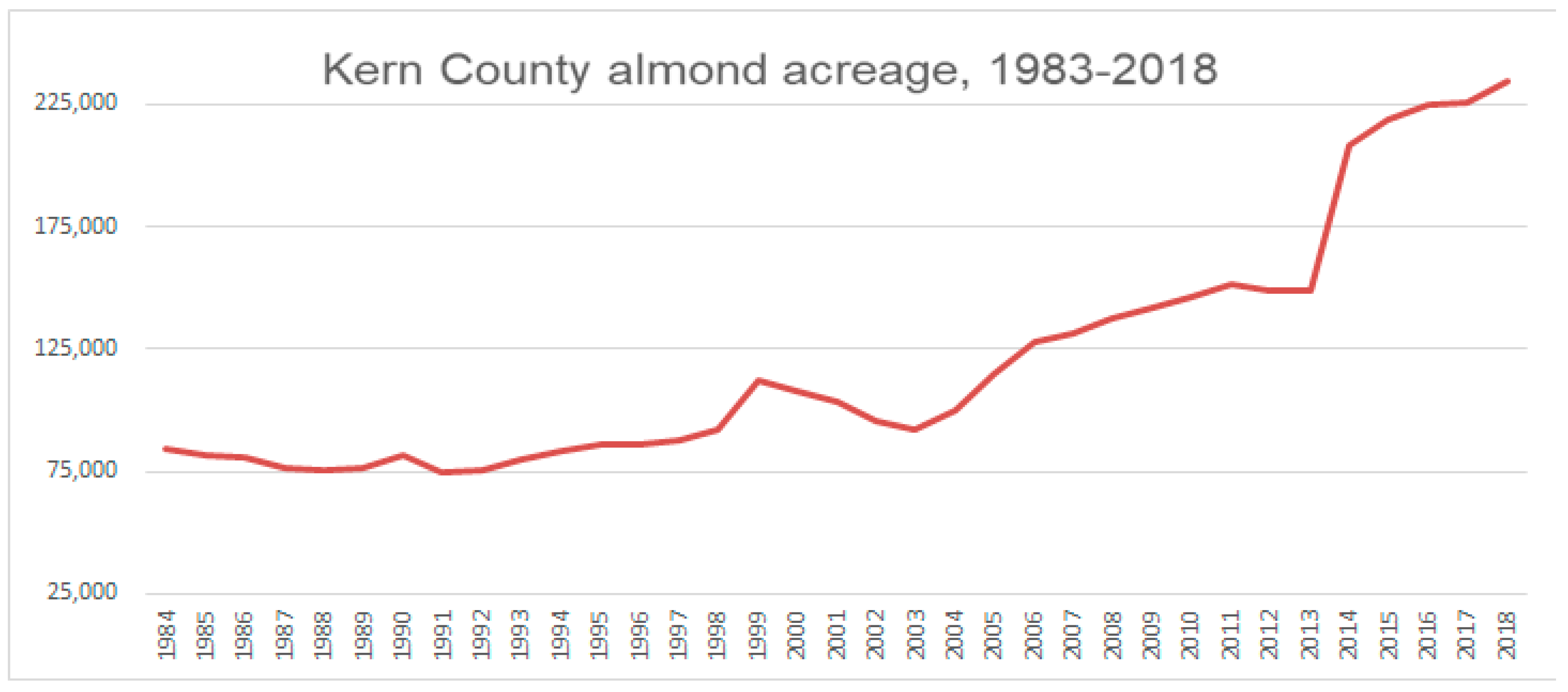
The analysis is for Kern County, California, which has an area of 1 million acres overlying usable groundwater and agricultural production limited to 0.9 million acres [24,25]. This region has access to high-quality surface water imports from a variety of sources, but groundwater also represents a significant source of supply to agricultural production. Kern County is a major producer of fruit and nut crops, among which crop area devoted to almonds has increased significantly over the last 20 years, concurrently with almond prices, and particularly since 2013 (Figure 1).
The average land use, agricultural prices, and cost budget, for all crops, are drawn from the Kern County agricultural reports [25,29], as well as almond lifecycle, and age-dependent inputs and related costs. Healthy almond trees remain in commercial production for approximately 22–25 years. They do not bear any yields in the first 2 years and only reach maturity (full yields) at age 6. It is also assumed that yields decline linearly after age 20, a stylized approximation of the observation that older perennial crops tend to decline in productivity after a certain age. A summary of the age-dependent parameters is presented in Table 4.
Production costs for both annual and perennial crops include capital recovery costs, irrigation system purchase and operating and maintenance costs (including taxes), insurance and estimated repair costs, and planting, cultivation, fertilization, and pesticide application costs. Harvest and production costs are from [22,29] with inflation adjustment. All monetary values are in 2016 dollars. Baseline parameter values are presented in Table 5.
2.6. Computational Model
The model is formulated as a dynamic, non-linear programming optimization problem and solved in GAMS using the CONOPT4 solver. Model dynamics are handled using a running horizon algorithm [30], which simulates an infinite-horizon dynamic programming problem. The model is calibrated using quadratic costs (as in PQP [23]) that increase with total area planted for both the perennial crop and each annual crop.
3. Results
3.1. Baseline
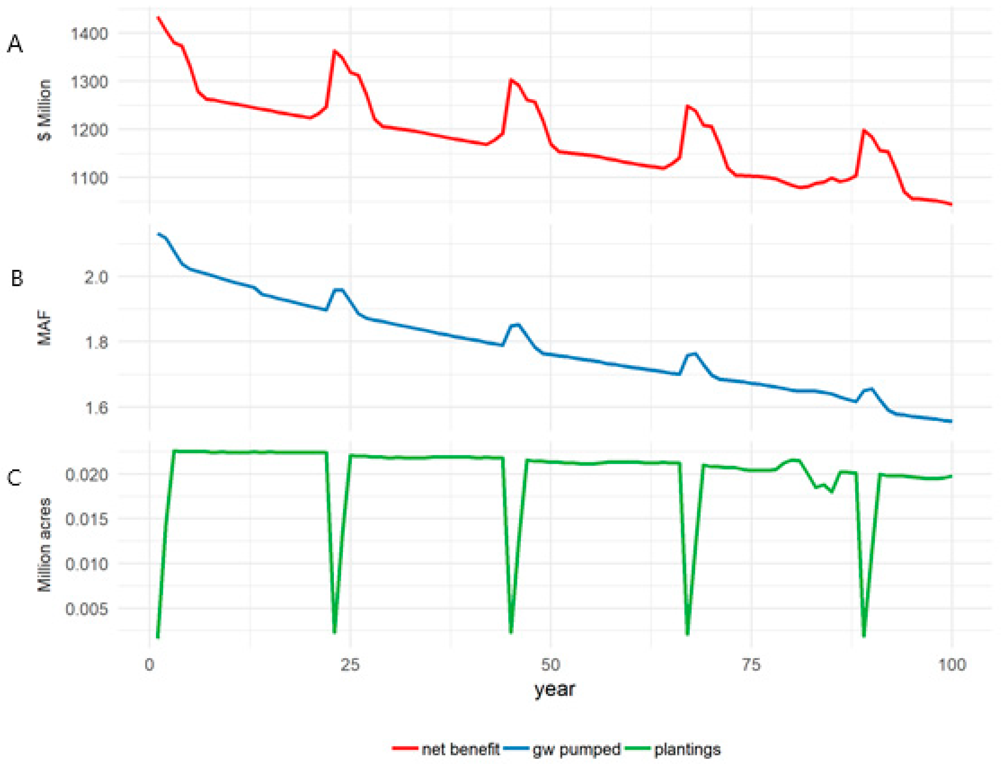
In this section, the dynamic model is run over a 100-year horizon on the baseline scenario, which assumes a perennial price of USD 2.53 per pound and 1.97 MAF of surface water available. Figure 2 shows the annual net benefits along with groundwater pumping and perennial plantings. Although other factors such as annual crop production and groundwater pumping costs factor into changes in benefits over time, the peaked nature of the annual net benefits time series follows directly from changes in the management of the perennial crop. Both net benefits and groundwater pumping spike in periods in which relatively less non-bearing almond area is in production. That is, underlying the aggregate perennial acreage, there is a constantly evolving age distribution of trees which is managed by plantings and removals. Both benefits and water requirements are higher with mature perennials, and therefore any period in which mature trees are slightly over-represented results in spikes, as seen here. The influence of replacement echoes in perennial crop area can be seen in the spikes in groundwater pumping, which decline over time as the age distribution smooths out. Groundwater pumping starts at around 2 AF per acre and steadily declines over time as the aquifer level drops and pumping costs increase. By the last time period, pumping levels are reduced to 1.5 AF per acre, and the aquifer is approximately 270 feet lower than in the first period, representing a draw-down of approximately 2.7 feet per year.
There are no plantings or removals of perennials in the first year, and subsequent plantings and removals (not shown) are in balance until year 23 when both fall to almost zero again. As perennials are replanted, there is a smoothing out of the land distribution across age classes such that, eventually, the model, ceteris paribus, will converge to completely smooth planting and removal time series. This finding is consistent with [31] and [12], although it should be noted that the smoothing in those papers follows from the use of a non-linear utility function, whereas here, it results from the model’s calibration.
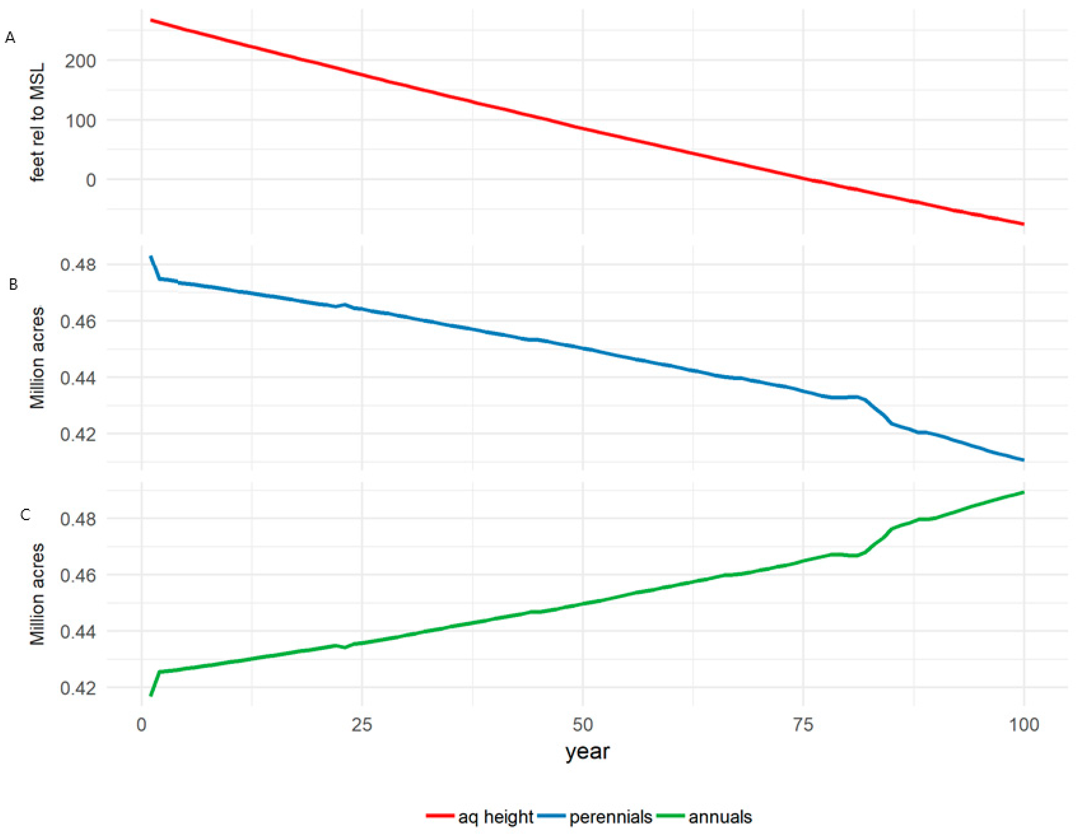
To further demonstrate the behavior of the model, Figure 3 shows the time series of the aquifer level and land use by crop type. Consistent with Figure 2, groundwater pumping steadily draws down the aquifer, resulting in higher pumping costs over time. Those costs then translate to a decrease in the area devoted to the more water-intensive perennial crop in favor of annual crops with no land left fallow in any time period.
3.2. Water Reductions
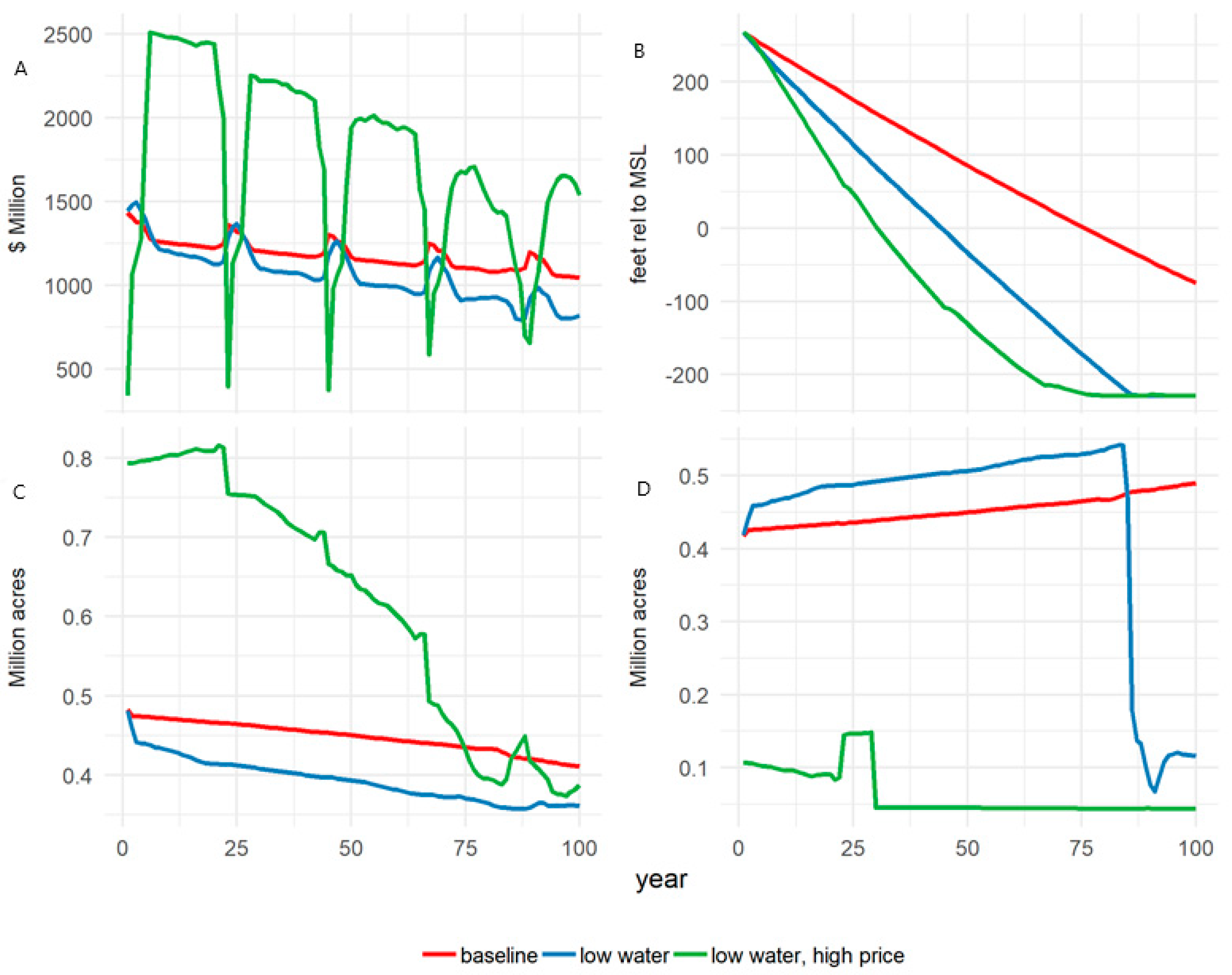
While no one knows precisely how climate change coupled with drought will impact future water supply availability for irrigated agriculture, agricultural regions in California, and likely throughout the world, likely will need to reduce water use to bring their basins into balance [32]. In this section, we investigate the impact of a permanent surface water reduction with and without a corresponding change in perennial prices for a 100-year horizon (referred to as “low water” and “low water, high price”, respectively). The reduction in surface water is assumed to be 25% relative to the baseline for a total annual supply of approximately 1.48 MAF. The perennial price increase is assumed to be 25%, for approximately USD 3.16 per pound.
Figure 4 depicts key time series for the “low water” and “low water, high price” scenarios. The corresponding results from the baseline scenario are also included for comparison. The annual net benefits in the “low water” and “low water, high price” scenarios are lower and higher than the baseline, respectively (USDM 1059 and USDM 1804 vs. USDM 1173). Perennial area in the “low water” scenario is about 40,000 acres lower than the baseline (396,000 vs. 436,000 acres) and approximately 219,000 acres (635,000) higher in the “low water, high price” scenario. Whereas the decline in perennial area in the “low water” scenario is rather muted, the change in the “low water, high price’ scenario is dramatic, falling by more than half (400,000 acres) over the 100-year time horizon. The apparent implication is that surface water reductions eventually lead to a decrease in perennial area, but a higher perennial price provides a strong incentive to start at a much higher level of perennial production. While annual crop area increases over time in the “low water” scenario over much of the time horizon, it eventually collapses due to high pumping costs. In contrast, annual crops are almost crowded out by perennials in the “low water, high price” scenario, with a spike in annual area occurring around year 25 as much of the perennial area is removed. Beyond that, the relatively high profitability of perennials and high pumping costs lead annual crop area to be drawn down to almost nothing by the end of the horizon. Both water reduction scenarios dramatically draw down the aquifer relative to the baseline, with each almost de-watering the aquifer at a height of −229 below MSL as compared to −12 feet in the baseline. The difference between the two water reduction scenarios is that the “low water, high price” scenario follows a steeper descent, dropping below −200 feet by approximately year 64, whereas the “low water” scenario does not do so until approximately year 87, again reflecting the reliance on groundwater to irrigate the large perennial crop area. While the baseline does not experience any fallowing, the “low water” and “low water, high price” scenarios experience high levels of fallowing in the last period with 371,000 and 436,000 acres fallowed, respectively.
3.3. Model Comparison
In this section, we consider two alternate ways of modeling perennial crops in which perennial area is either held fixed over time (“fixed”) or is assumed to be completely flexible from year to year (“as annual”) with costless area adjustment. The “fixed” model is the same as the “dynamic” model developed above except that perennial area is held constant at st = 504,000 acres, and age 10, representing a mature crop, is assumed for all age-dependent parameters. As a result, Equations (7) and (8) describing perennial dynamics are irrelevant as is the removal variable, which is set to zero (zkt = 0). Relatedly, a fraction of the cost of crop removal is deducted each year under the assumption of a 22-year productive lifecycle. (In general, the optimal rotation length is a function of groundwater management and other variables and hence cannot be determined precisely for an equivalent non-dynamic perennial model; however, given the age–yield relationship assumed here, a rotation length ranging from 21 to 25 years is very likely.) The “as annual” version of the model is essentially the same as the “fixed” model except that perennial area can take any level (St ∈ (0–900,000) acres).
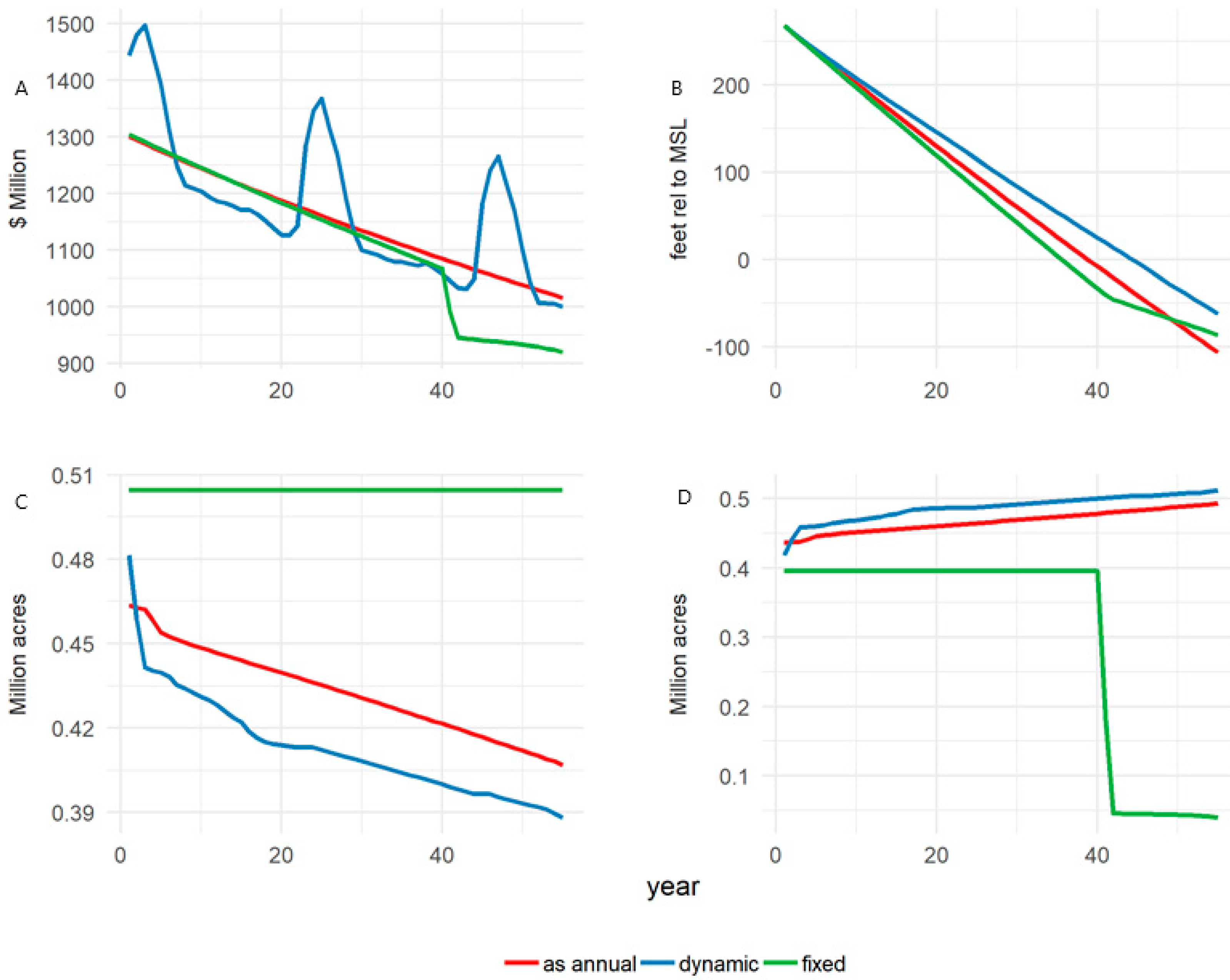
Since the results for several scenarios using the fixed model de-water the aquifer and result in model infeasibilities for periods longer than 55 years, to be consistent, we use a 55-year time horizon for comparison across models and scenarios for all results in this section. Figure 5 depicts the time series of key variables in the baseline scenario. Given the lack of perennial crop dynamics in the two alternate models, the annual net benefits smoothly decline over time, with median values slightly lower than the “dynamic” model (approximately USDM 1219, 1214, and 1233 for “as annual”, “fixed”, and “dynamic” models, respectively). Aquifer draw-down is significantly less in the “dynamic” model than in the other two, partially due to the lower water requirements of immature perennials, while the final aquifer height is approximately 35 and 7 feet, respectively, for the “as annual” and “fixed” models. On a per-year basis, this translates to median pumping volumes of 1.87 MAF for the “dynamic” model vs. 1.97 and 2.03 MAF for the “as annual” and “fixed” models. As groundwater pumping becomes more expensive over time, there is a corresponding shift away from water-intensive perennials and toward annual crops for the both the “dynamic” and “as annual” models, but not for the “fixed” model. The downward adjustment of perennial area is more immediate in the “as annual” model and then accelerates toward the end of the time horizon relative to the “dynamic” model, reflecting, again, the stickiness of investment in the “dynamic” model. Note that there is no fallowing across all three models and that land use by crop type (perennial vs. annual crops) for the “dynamic” model is bounded by the land use results from the other two models—the “fixed” model has a higher perennial and a lower annual crop area, while the reverse is true for the “as annual” model.
The results from the “low water” scenario for each model are shown in Figure 6. Similar to the results from the baseline scenario, the “dynamic” model displays slightly higher median annual net benefits (approximately USDM 1145, 1136, and 1163 for “as annual”, “fixed”, and “dynamic” models, respectively) and less draw-down of the aquifer (heights of approximately 74, 58, and 96 feet relative to MSL for “as annual”, “fixed”, and “dynamic” models, respectively). While the “as annual” and “dynamic” models show similar trends of substituting annual crops for perennials over time, they are reversed relative to the baseline scenario in that the “dynamic” model is more aggressive about replacing perennials, whereas in the baseline, the opposite is true. The “fixed” model holds annual crop area constant until year 40 when it collapses to almost zero, a pattern that is repeated in Figure 7 because the “fixed” model has no flexibility to take advantage of higher perennial prices. In contrast, the “as annual” and “dynamic” models take advantage of higher prices by dramatically increasing perennial crop area to close to 800,000 acres in the first year. Whereas the “as annual” model makes a smooth, continuous transition away from perennials over the whole time horizon, the perennial rotation dynamics results in a stable to slightly increasing trend in perennial area until after year 20 when removals of older crops result in a discrete drop in area. Perennial area continues to be drawn down over the rest of the time horizon, but changes in area continue to be bumpy due to differences in the area of different vintages. Again, in this scenario, the “dynamic” model has the highest median annual net benefits with a difference of USDM 397 and USDM 432 compared to the “as annual” and “fixed” models, respectively.
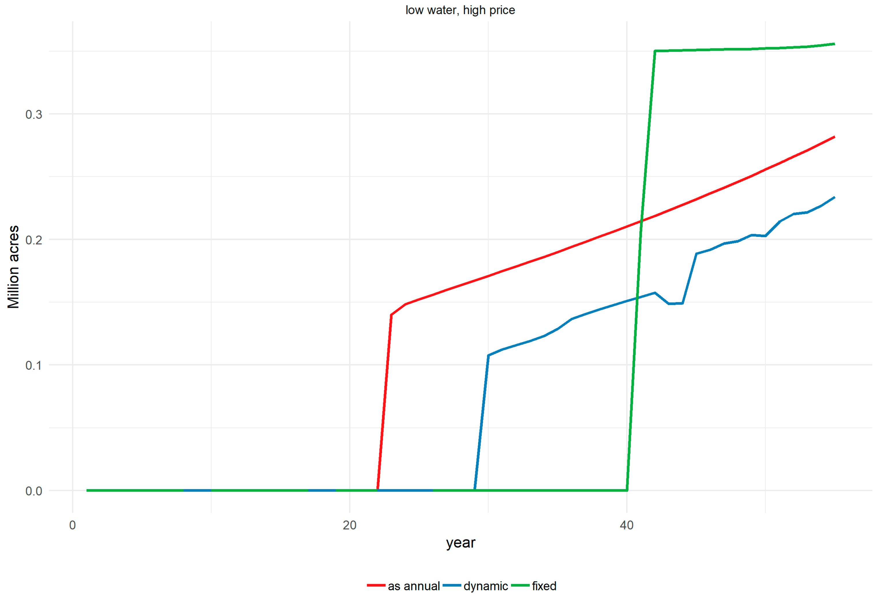
Other variables initially identified as being key ways to adapt to drought are land fallowing and groundwater pumping. Land fallowing occurs in the “low water” scenario only for the “fixed” model, but it varies significantly across models in the “low water, high price” scenario. As seen in Figure 8, the “as annual” model begins fallowing first in year 22 and increases fallowed area smoothly over the rest of the time horizon. The “dynamic” model starts later but follows a similar pattern, while the fixed model has an abrupt transition with 350,000 or more acres fallowed from year 42 onward, which is identical to the behavior in the “low water” scenario. As opposed to fallowing, differences in aquifer draw-down vary much more across scenarios, with the “dynamic” model drawing down the aquifer the least in all scenarios except for the “low water, high price” case. The range in draw-down across the baseline, “low water”, and “low water, high price” scenarios is approximately 62, 44, and 77 feet, respectively, amounting to average differences ranging from approximately 0.8 to 1.4 feet per year.
4. Discussion
In comparing the results for each of the model versions across all scenarios, some patterns emerge. Modest differences in the present value of the net benefits (PVNB) between the baseline and “low water” scenario (Table 6) for each model suggest that benefits are not very sensitive to water reductions per se. This may follow because there are numerous ways to adapt to surface water shortages included in the analysis: land fallowing, increased groundwater pumping, switching annual crops, and switching irrigation systems for annual crops. Clearly, as the options to adapt diminish, PVNB will likely be more sensitive to water reductions.
The biggest determinant of PVNB captured by these scenarios is, by far, the high perennial price in the “less surface water, high price” scenario. As seen above, this shifts production toward perennials despite increased pumping costs in a way that is consistent with recent experiences in California. The lack of fallowing in the baseline and “low water” scenarios indicates that, absent management rules to the contrary, adaptation to water shortages in this framework favors increased groundwater pumping over land fallowing—a result consistent with recent experiences in California. While the inability to deficit irrigate the perennial crop in the model may be a factor favoring increased pumping, reliance on groundwater seems to be a result of the fundamental economics of the problem faced by irrigators. That is, it is difficult to draw down the aquifer enough such that pumping costs become the primary determinant of production decisions, at least for the electricity price and time horizon considered here. It should be noted that this analysis assumes efficient management of the aquifer in a deterministic environment. It may be the case that either common property management, uncertainty, or the combination of the two could reverse this finding.
As we have seen, except for the “less surface water, high price” scenario, the “dynamic” model draws down the aquifer significantly less than the other models. This finding may not match the reader’s intuition as the more realistic representation of perennial crop dynamics might be expected to lead to demand hardening in the sense that the need to protect mature, productive perennials could put more pressure on the aquifer. While that may hold in the short run in a stochastic analysis, it does not hold in the long-run analysis here. Instead, it appears that given perfect foresight and the ability to efficiently manage the use of groundwater, the “dynamic” model accounts for future aquifer conditions when making perennial crop planting and removal decisions. Although it is understood that planting decisions early in the time horizon have an effect on the evolution of the aquifer potentially as long as 25 years later, it is also true that in a dynamic equilibrium, the expected future conditions inform decision making in earlier periods.
Lastly, the “dynamic” model’s more realistic representation of perennial crop production seems to result in more realistic land use patterns across scenarios. While the “fixed” model exhibits unrealistically abrupt land use transitions, the “as annual” model has very smooth transitions, as highlighted in the case of the “low water, high price” scenario. In contrast, the “dynamic” model has rigidities built into perennial crop production and exhibits oscillations that have long been noted in studies of the supply of different perennial crops [33,34].
5. Conclusions
To the authors’ knowledge, this study is one of the few, if not the first, that combines the economic dynamics of perennial crops and groundwater management, thus extending the literature on both topics. Characteristics of perennial crops including large fixed costs from planting, multi-year periods of establishment and senescence, and age-dependent productivity and input requirements are all included in the model here. The resulting transitional dynamics imply a strong incentive to pump groundwater in the face of surface water reductions, which may be exacerbated by market pressures favoring perennial crops. Moreover, the analysis shows that simpler models used in the literature are, by construction, limited in their ability to capture such effects and therefore may not be reliable aids for policy analysis in periods of water scarcity.
This study used one of the most common calibration techniques in the literature (PMP) and applied it to a dynamic setting to highlight how the representation of perennial crops might impact outcomes. Yet, whereas PMP calibrates to a reference year exactly for a static optimization problem, the approach taken here can only ensure an approximate calibration of crop area to a reference level due to the evolution of the perennial and groundwater stock variables over time. The development of a more general calibration method that accounts for the dynamics in this model is a topic for further research.
Given the rarity of models that account for perennial dynamics, it is likely that policymakers will be ill informed as to how irrigated agriculture and groundwater systems co-evolve, especially when the perennial crop acreage is significant. Particularly given the likely impacts of climate change in California, this underscores the need for further research on the economics of irrigated perennial crops and their influence on groundwater pumping. The results presented here indicate that including the dynamics of both perennial crops and groundwater levels can have a significant impact on the water demand for irrigation and land use transitions over time. A better understanding of such issues may help policymakers anticipate likely changes in irrigated agriculture in areas affected by California’s SGMA regulations, especially since established perennial crops are likely to factor heavily into land and water acquisitions during SGMA’s transitional period until 2040.
Author Contributions
Conceptualization, B.F. and K.S.; methodology, B.F. and K.S.; software, B.F.; validation, B.F.; formal analysis, B.F.; investigation, B.F.; resources, K.S.; data curation, B.F. and L.L.; writing—original draft preparation, B.F.; writing—review and editing, B.F., K.S., L.L.; visualization, B.F.; supervision, K.S.; project administration, B.F.; funding acquisition, K.S. All authors have read and agreed to the published version of the manuscript.
Funding
This research was partially supported by the UCR NSF INFEWS grant titled “INFEWS/T3: Decision Support for Water Stressed FEW Nevus Decisions (DS-WSND)”.
Institutional Review Board Statement
Not Applicable.
Informed Consent Statement
Not Applicable.
Data Availability Statement
Not Applicable.
Conflicts of Interest
The authors declare no conflict of interest.
References
- Loukas, A.; Vasiliades, L.; Tzabiras, J. Climate change effects on drought severity. Adv. Geosci. 2008, 17, 23–29. [Google Scholar] [CrossRef] [Green Version]
- Mahmoudi, M.H.; Najafi, M.R.; Singh, H.; Schnorbus, M. Spatial and temporal changes in climate extremes over northwestern North America: The influence of internal climate variability and external forcing. Clim. Chang. 2021, 165, 1–19. [Google Scholar] [CrossRef]
- Howitt, R.E.; MacEwan, D.; Medellin-Azuara, J.; Lund, J.R.; Sumner, D.A. Economic Analysis of the 2015 Drought for California Agriculture; Center for Watershed Sciences: Davis, CA, USA, 2015; p. 16. [Google Scholar]
- ABS. Water Use on Australian Farms. 2008–2009. Available online: https://www.abs.gov.au/AUSSTATS/[email protected]/Lookup/4618.0Main+Features12008-09 (accessed on 1 April 2019).
- Schwabe, K.; Connor, J. Drought issues in semi-arid and arid environments. Choices 2012, 27, 5. [Google Scholar]
- Rohde, M.M.; Froend, R.; Howard, J. A global synthesis of managing groundwater dependent ecosystems under sustainable groundwater policy. Groundwater 2017, 55, 293–301. [Google Scholar] [CrossRef] [PubMed]
- Faunt, C.C.; Sneed, M.; Traum, J.; Brandt, J.T. Water availability and land subsidence in the central valley, California, USA. Hydrogeol. J. 2016, 24, 675–684. [Google Scholar] [CrossRef] [Green Version]
- Nelson, T.; Chou, H.; Zikalala, P.; Lund, J.; Hui, R.; Medellin-Azuara, J. Economic and water supply effects of ending groundwater overdraft in california’s central valley. San Fr. Estuary Watershed Sci. 2016, 14. [Google Scholar] [CrossRef] [Green Version]
- Hanak, E.; Escriva-Bou, A.; Gray, B.; Green, S.; Harter, T.; Jezdimirovic, J.; Lund, J.; Azuara, J.M.; Moyle, P.; Seavy, N. Water and the Future of the San Joaquin Valley; Public Policy Institute of California: San Francisco, CA, USA, 2019. [Google Scholar]
- Sustainable Groundwater Management Act (SGMA). 2014. Available online: https://water.ca.gov/Programs/Groundwater-Management/SGMA-Groundwater-Management (accessed on 1 April 2019).
- CalAg. California Agricultural Statistics 2018. 2018. Available online: https://www.cdfa.ca.gov/Statistics/PDFs/2017-18AgReport.pdf (accessed on 1 April 2019).
- Franklin, B.; Knapp, K.C.; Schwabe, K.A. A dynamic regional model of irrigated perennial crop production. Water Econ. Policy 2017, 3, 1650036. [Google Scholar] [CrossRef]
- Marques, G.; Lund, J.; Howitt, R. Modeling irrigated agricultural production and water use decisions under water supply uncertainty. Water Resour. Res. 2005, 41, W08423. [Google Scholar] [CrossRef]
- Connor, J.; Schwabe, K.; King, D.; Kaczan, D.; Kirby, M. Impacts of climate change on lower Murray irrigation. Aust. J. Agric. Resour. Econ. 2009, 53, 437–456. [Google Scholar] [CrossRef]
- Adamson, D.; Loch, A.; Schwabe, K. Adaptation responses to increasing drought frequency. Aust. J. Agric. Resour. Econ. 2017, 19, 385–403. [Google Scholar] [CrossRef] [Green Version]
- Swegal, H. The Rise and Fall of Almond Prices: Asia, Drought, and Consumer Preference. 2017. Available online: https://hdl.handle.net/1813/78294 (accessed on 1 April 2019).
- Booker, F.J.; Young, R.A. Modeling intrastate and interstate markets for Colorado river water resources. J. Environ. Econ. Manag. 1994, 26, 66–87. [Google Scholar] [CrossRef]
- Howitt, R.; MacEwan, D.; Medellin-Azuara, J.; Lund, J. Economic Modelling of Agriculture and Water in the California Using the Statewide Agricultural Production Model; University of California: Davis, CA, USA, 2010. [Google Scholar]
- Rosegrant, M.W.; Ringler, C.; McKinney, D.C.; Cai, X.; Keller, A.; Donoso, G. Integrated economic-hydrologic water modeling at the basin scale: The Maipo river basin. Agric. Econ. 2000, 24, 33–46. [Google Scholar]
- Ward, A.F.; Michelsen, A. The economic value of water in agriculture: Concepts and policy applications. Water Policy 2002, 4, 423–446. [Google Scholar] [CrossRef]
- Zhu, T.; Marques, G.F.; Lund, J.R. Hydroeconomic optimization of integrated water management and transfers under stochastic surface water supply. Water Resour. Res. 2015, 51, 3568–3587. [Google Scholar] [CrossRef]
- Schwabe, K.A.; Kan, I.; Knapp, K.C. Drainwater management for salinity mitigation in irrigated agriculture. Am. J. Agric. Econ. 2006, 88, 133–149. [Google Scholar] [CrossRef]
- Howitt, R.E. Positive mathematical programming. Am. J. Agric. Econ. 1995, 77, 329–342. [Google Scholar] [CrossRef]
- DWR. San Joaquin Valley Groundwater Basin Kern County Subbasin. Available online: https://water.ca.gov/-/media/DWR-Website/Web-Pages/Programs/Groundwater-Management/Bulletin-118/Files/2003-Basin-Descriptions/5_022_14_KernCountySubbasin.pdf (accessed on 1 April 2019).
- Kern. 2017 Kern County Agriculture Report. 2017. Available online: http://www.kernag.com/caap/crop-reports/crop10_19/crop2017.pdf (accessed on 11 April 2019).
- Knapp, K.; Baerenklau, K.A. Ground water quantity and quality management: Agricultural production and aquifer salinization over long time scales. J. Agric. Resour. Econ. 2006, 31, 616–641. [Google Scholar]
- Kern. 2018 Kern County Agriculture Report. 2018. Available online: http://www.kernag.com/caap/crop-reports/crop10_19/crop2018.pdf (accessed on 15 April 2021).
- Kern. 2019 Kern County Agriculture Report. 2019. Available online: http://www.kernag.com/caap/crop-reports/crop10_19/crop2019.pdf (accessed on 15 April 2021).
- UCDavis. Archived Cost and Return Studies. 2019. Available online: https://coststudies.ucdavis.edu/en/archived/ (accessed on 11 April 2019).
- Knapp, K.C.; Schwabe, K.A. Spatial dynamics of water and nitrogen management in irrigated agriculture. Am. J. Agric. Econ. 2008, 90, 524–539. [Google Scholar] [CrossRef]
- Franklin, B. The Dynamics of Irrigated Perennial Crop Production with Applications to the Murray-Darling Basin of Australia. Ph.D. Thesis, University of California, Riverside, CA, USA, 2013. [Google Scholar]
- Mount, J.; Hanak, E.; Baerenklau, K.; Butsic, V.; Chappelle, C.; Escriva-Bou, A.; Fogg, G.; Gartrell, G.; Grantham, T.; Gray, B.; et al. Managing Drought in a Changing Climate: Four Essential Reforms; Public Policy Institute of California Water Policy Center: Sacramento, CA, USA, 2018. [Google Scholar]
- French, B.C.; Bressler, R.G. The lemon cycle. J. Farm Econ. 1962, 44, 1021–1036. [Google Scholar] [CrossRef]
- Knapp, K.C. Dynamic equilibrium in markets for perennial crops. Am. J. Agric. Econ. 1987, 69, 97–105. [Google Scholar] [CrossRef]

Figure 2.
Baseline scenario. (A) annual net benefits, (B) groundwater pumped, and (C) perennial plantings.
Figure 2.
Baseline scenario. (A) annual net benefits, (B) groundwater pumped, and (C) perennial plantings.

Figure 3.
Baseline scenario, where the rows (from top) are the (A) aquifer level, (B) perennial area, and (C) annual area.
Figure 3.
Baseline scenario, where the rows (from top) are the (A) aquifer level, (B) perennial area, and (C) annual area.

Figure 4.
Key time series for “baseline”, “low water”, and “low water, high price” scenarios. (A) annual net benefits, (B) aquifer height, (C) perennial area, and (D) annual area.
Figure 4.
Key time series for “baseline”, “low water”, and “low water, high price” scenarios. (A) annual net benefits, (B) aquifer height, (C) perennial area, and (D) annual area.

Figure 5.
Model comparison under baseline scenario, key time series. (A) annual net benefits, (B) aquifer height, (C) perennial area, and (D) annual area.
Figure 5.
Model comparison under baseline scenario, key time series. (A) annual net benefits, (B) aquifer height, (C) perennial area, and (D) annual area.

Figure 6.
Model comparison of key series for the “low water” scenario. (A) annual net benefits, (B) aquifer height, (C) perennial area, and (D) annual area.
Figure 6.
Model comparison of key series for the “low water” scenario. (A) annual net benefits, (B) aquifer height, (C) perennial area, and (D) annual area.

Figure 7.
Model comparison for key time series in the “low water, high price” scenario. (A) annual net benefits, (B) aquifer height, (C) perennial area, and (D) annual area.
Figure 7.
Model comparison for key time series in the “low water, high price” scenario. (A) annual net benefits, (B) aquifer height, (C) perennial area, and (D) annual area.

Figure 8.
Fallowing in the “low water, high price” scenario.


Table 1.
Sample of agricultural programming models of arid and semi-arid regions.
| Study | Region | Perennials? | Dynamic? |
|---|---|---|---|
| Adamson et al. (2017) [15] | Murray–Darling Basin | Yes | 2-stage |
| Booker and Young (1994) [17] | Colorado River | No | No |
| Connor et al. (2009) [14] | Murray–Darling Basin | Yes | 2-stage |
| Franklin et al. (2017) [12] | Murray–Darling Basin | Yes | Fully dynamic |
| Howitt et al. (2010) [18] | California | No | No |
| Marques et al. (2005) [13] | California | Yes | 2-stage |
| Rosegrant et al. (2000) [19] | Maipo Valley, Chile | No | No |
| Ward and Michelsen (2002) [20] | Rio Grande | No | No |
| Zhu et al. (2015) [21] | Mediterranean | Yes | 2-stage |
Table 2.
Crop area reference levels for calibration.
| Crop | Reference Level (Million Acres) |
|---|---|
| Almonds | 0.504 |
| Alfalfa | 0.253 |
| Cotton | 0.104 |
| Tomatoes | 0.042 |
| Wheat | 0.062 |
| Fallow | 0.045 |
Table 3.
Key model components.
| Variable | Interpretation | Units |
|---|---|---|
| πt | Agricultural profit | USD/acre |
| π0t | Perennial planting cost | USD/acre |
| πst | Perennial profit | USD/acre |
| πxt | Annual crop profit | USD/acre |
| ht | Aquifer height | feet relative to MSL |
| skt | Perennial area for age k | acres |
| xijt | Annual crop area | acres |
| wijt | Water applied to annual crops | AF/acre |
| zkt | Removals for age k perennial | acres |
| Index | ||
| i | Annual crop | |
| j | Irrigation system | |
| k | Perennial age | |
| dp | Deep percolation | |
| gw | Groundwater | |
| sw | Surface water | |
| t | Year | |
| Parameter | ||
| α | Discount factor | |
| r | Discount rate | |
| γk | Cost for age k perennial | USD/acre |
| γgw,t | Groundwater cost | USD/AF |
| γsw,t | Surface water cost | USD/AF |
| γz | Removal cost for perennials | USD/acre |
| γx | Cost for annual crop | USD/acre |
| γscal | Perennial calibration cost | USD/acre |
| γxcal | Annual crop calibration cost | USD/acre |
| p | Crop price | USD/lb |
| q | Water volume | AF |
| wk | Water required for perennial age k | AF/acre |
| y | Crop yield | lbs/acre |
Table 4.
Age-dependent parameter values for almonds.
| Age | Yield | Water Req. | Non-Water Cost |
|---|---|---|---|
| (lbs./Acre) | (Acre-Inches) | (USD per Acre) | |
| 1 | 0 | 11 | 3432 |
| 2 | 0 | 21 | 918 |
| 3 | 400 | 32 | 1684 |
| 4 | 800 | 42 | 2392 |
| 5 | 1600 | 42 | 2523 |
| 6–21 | 2246 | 42 | 2601 |
| 22 | 2021.4 | 42 | 2601 |
| 23 | 1796.8 | 42 | 2601 |
| 24 | 1572.2 | 42 | 2601 |
| 25 | 1347.6 | 42 | 2601 |
Table 5.
Baseline parameter values.
| Parameter | Symbol | Value | Units |
|---|---|---|---|
| Initial Aquifer Level | 268 | Feet relative to MSL | |
| Initial Perennial Area | 0.45 | Proportion of total land | |
| Perennial Crop Price | 2.53 | USD per lb. | |
| Surface Water Available | 1.97 | AF | |
| Surface Water Cost | 65 | USD per AF | |
| Energy Cost | 0.148 | USD | |
| Discount Rate | 0.05 | - |
Table 6.
Present Value Net Benefit by scenario and model.
| Scenario | Model | PVNB ($ M) |
|---|---|---|
| baseline | as annual | 24,535 |
| dynamic | 24,965 | |
| fixed | 24,493 | |
| low water | as annual | 23,644 |
| dynamic | 24,329 | |
| fixed | 23,439 | |
| low water, high price | as annual | 37,254 |
| dynamic | 37,897 | |
| fixed | 34,880 |
Publisher’s Note: MDPI stays neutral with regard to jurisdictional claims in published maps and institutional affiliations. |
© 2021 by the authors. Licensee MDPI, Basel, Switzerland. This article is an open access article distributed under the terms and conditions of the Creative Commons Attribution (CC BY) license (https://creativecommons.org/licenses/by/4.0/).
Share and Cite
MDPI and ACS Style
Franklin, B.; Schwabe, K.; Levers, L. Perennial Crop Dynamics May Affect Long-Run Groundwater Levels. Land 2021, 10, 971. https://doi.org/10.3390/land10090971
AMA Style
Franklin B, Schwabe K, Levers L. Perennial Crop Dynamics May Affect Long-Run Groundwater Levels. Land. 2021; 10(9):971. https://doi.org/10.3390/land10090971
Chicago/Turabian StyleFranklin, Bradley, Kurt Schwabe, and Lucia Levers. 2021. "Perennial Crop Dynamics May Affect Long-Run Groundwater Levels" Land 10, no. 9: 971. https://doi.org/10.3390/land10090971
Note that from the first issue of 2016, this journal uses article numbers instead of page numbers. See further details here.