Applying the Hubbard-Stratonovich Transformation to Solve Scheduling Problems Under Inequality Constraints With Quantum Annealing

1 Introduction

Since being first proposed by Richard Feynman in 1981, quantum computing has been an intriguing idea for both physicists and computer scientists [1]. The core concept of a quantum computer is to manipulate a quantum system in a large Hilbert space in order to gain a significant advantage over classical computing to solve certain classes of hard problems. For instance, it has been theoretically proven that quantum algorithms bring an exponential speed-up over traditional methods on the problems of factorization [2] and quantum simulation [3, 4], as well as a quadratic speed-up for unstructured search [5].

For many hard computational problems however, no approach, either classical or quantum, has been theoretically proven to outperform others. In practice, the investigation of quantum advantage is thus closely related to hardware development in order to obtain empirical evidence. Yet, controlling and manufacturing a quantum computer remains an unsolved challenge, although past decades have witnessed multiple breakthroughs. Despite the recently achieved significant milestones for quantum computing, with quantum supremacy tests being performed (Google’s superconducting quantum computer Sycamore [6], photonic quantum computer JiuZhang [7]), it is still a fundamental research question to determine which problems and applications should be solved more efficiently by using quantum computing in place of classical computers; and to what extent. Given the current technological advancement, quantum annealing-a metaheuristic optimization algorithm-achieves promising experimental performances in finding near-optimal solutions for some NP-hard optimization problems [8–11]. Quantum annealing requires to map an optimization problem to an Ising spin glass model with Hamiltonian H_P, to which QPUs are restricted to by construction, and then solve the problem by sampling the low-energy states of the physical system. The system is typically initialized in the ground state of an easy-to-implement driver Hamiltonian H_D, and then evolved progressively towards H_P:

where A(0) = 1, B(0) = 0 and B(1) = 1, A(1) = 0. With σ^x, σ^z the Pauli spin operators and $J_{ij},h_i^z,h_i^x$ some scalar coefficients, the problem Hamiltonian with n qubits is written $H_p={\sum }_{<i,j>}{J}_{ij}{\sigma }_i^z{\sigma }_j^z+{\sum }_{i=1}^n{h}_i^z{\sigma }_i^z$ while the driver Hamiltonian $H_D={\sum }_{i=1}^n{h}_i^x{\sigma }_i^x$ does not commute with H_P, thus creating the quantum fluctuations. The annealing process, which is a dynamic process of the quantum system, is non-trivial and techniques such as non-linear scheduling, pausing and reverse-annealing can further improve the quality of the final system state [12, 13].

The understanding of the underlying physical process and the speed-up that quantum annealing could provide over classical methods has been a heated topic of debate and interest. Indeed, the notion of quantum speed-up itself has been proven to be elusive, and varies from provable to limited speed-ups, depending on the question that is investigated [14–16]. It has been commonly believed that quantum annealing can exhibit speed-up over simulated annealing due to the fact that it can escape local minima via quantum tunneling effect [17]. However, some research is still needed to clarify to what extent quantum tunneling can accelerate the optimization process. Besides, another issue is whether the quantum tunneling effect can be observed in the current physical device. Finally, it has been shown that the speed-up of quantum annealing could be highly dependent on the high dimensional energy landscape determined by the problem structure [18].

Despite these key challenges, the rapid progresses achieved in hardware development suggest that practical applications of quantum computing are within reach. Particularly, the latest generation of D-Wave’s Quantum Processing Units (QPUs), designed to solve optimization problems with quantum annealing, reaches more than 5,000 qubits. As such, quantum annealing has already been applied to several real life problems with D-Wave’s experimental device. The applications range from scheduling and planning problems [19–21], machine learning [22, 23] and other domains such as molecular design [24, 25], portfolio optimization [26, 27] or robotic movement [28]. Notably, some experiments carried out on D-Wave’s 2000-qubit machine have shown that quantum annealing, when combined with classical solvers within an hybrid approach, can outperform some existing commercial solvers on industrial scale optimization problems, such as scheduling and traffic control [29, 30].

In this work, we are interested in solving an industrial energy problem, which can be written as a constrained integer programming problem: the optimal charging scheduling of electrical (EV) buses. Through this application, we aim at providing insights on two of the main research questions quantum annealing still needs to address, namely mapping to QUBO problems and embedding in hardware [19]. Due to the complex nature of the EV-bus charging problem, not tailored a priori for quantum computing, mapping to QUBO and then to hardware is effectively a costly step. In order to go beyond the penalty method commonly used for such mappings [31], we propose to use the Hubbard-Stratonovich transformation to obtain an efficient, with least qubit requirement, mapping. The transformation was first applied to quantum annealing problems by Ohzeki in 2020 [32], and we explore more deeply its practical implementation and performances by studying a problem of increased complexity, with several inequality constraints.

In the rest of this paper, we solve the EV bus charging scheduling problem on the D-Wave 2000q Quantum Processing Unit by firstly reformulating it into a QUBO problem with the penalty method, in Section 2. Besides, we also discuss the limitations of the penalty method, specifically the issues of graph connectivity and dynamic range. Next, by employing a method based on the Hubbard-Stratonovich transformation and described in Section 3, we reduce some of the quadratic penalties in the QUBO problem into linear terms, breaking thus the limitation of connectivity and dynamic range. Finally, we present and discuss some numerical experiments in Section 4 and conclude in Section 5.

2 EV-Bus Charging Scheduling Problem

2.1 Problem Definition

We consider a fleet of N_bus electrical buses and a set of N_pile piles. Assuming that the electricity consumption of all buses is known during their respective operating hours, the objective of the EV-bus charging scheduling problem is to find an optimal daily schedule for charging the buses by minimizing the cost of electricity while avoiding any breakdown. The EV-bus charging scheduling problem with minimization of price can thus be formulated as follows, with $\mathcal{T}=(t_1,t_2,\dots ,t_k,\dots ,t_T)$ being a discretization of time periods:

where z_ijk is a binary variable indicates whether bus i is charging at pile j for the time period t_k while o_ik = 0 if bus i is in operation and o_ik = 1 otherwise, i.e., if bus i is available for charging at time t_k. ω_j is the power output of pile j, p_k the cost of electricity at time t_k. We consider a time period of 24 h, and need only to find the values z_ijk during non-operating hours, i.e., during charging windows. This reduces the number of time steps to L_time ≤ T. In the sequel, we denote by S_il (respectively, D_il) the starting (respectively, ending) time of the l-th charging window of bus i. The constraints of the problem can be expressed as:

Constraint (3) ensures that any bus can only be charged at most one pile at a given time, while (4) means that the total number of buses being charged at the same time should not be greater than the total number of piles N_pile. (5) and (6) control the state-of-charge (SOC) of each bus i between 100 and 30% at all times by adding constraints at each time a bus leaves the charging station, with c_ik being the power consumption of bus i at time t_k. Note here that the power ω_j is also normalized to be consistent with SOC ∈ [0, 1]. Lastly (7) guarantees that a bus can only be charged continuously, and not intermittently, at most once during each charging window. Hence, the original EV-bus charging problem Eqs 2–7 is an integer programming problem with inequality constraints.

2.2 Reformulation of Constraints With the Penalty Method

Due to hardware constraints, quantum annealing can only be directly sampled from an Ising Hamiltonian. In this section, we reformulate thus the integer programming problem to a quadratic unconstrained binary optimization (QUBO) problem, which by definition does not include any constraint or non-binary variables [31, 33]. For each equality constraint of the form C_i(x) = 0 in the optimization problem, the penalty method consists in augmenting the cost function with a term $P_i^2(\mathbf{x})$ which penalizes the solutions that violate the constraint. For the inequality constraints, following [31], we first transform them into equality constraints with slack variables and then apply the penalty method. More specifically, constraints (3) and (7) are equivalent to

with s_1,ik, s_5,il ∈ {0, 1}. This yields the corresponding penalty functions:

It should be noted that Eq. 11 is of degree 4 in x, i.e, it is not a quadratic form. Therefore, a first limitation of the penalty method is that the already quadratic constraint (7) cannot be included in the augmented cost function.

Next, handling constraints (4) to (6) requires to introduce a slack variable that is either an integer [constraint (4)] or a real number [constraints (5)–(6)]. We choose to encode such non-binary variables s with binary encoding, i.e., $s=(1/\mathrm{\Gamma }){\sum }_{i=0}^{N-1}{2}^i{s}^{(i)},\mathrm{\Gamma }={\sum }_{i=0}^{N-1}{2}^i$, where N is the number of bits and upper-indexed s⁽ⁱ⁾ are used to denote the encoding binary variable of s. Other options, not explored in this article, for encoding the continuous variables include one-hot encoding and order encoding, as in [34]. Constraints (4)–(6) become

where s_2,jk is a binary-encoded integer slack variable in [0, N_pile] and s_3,il, s_4,il are binary-encoded continuous slack variables in [0, 1]. Furthermore, it is easy to see that the penalties P₃ and P₄ can be written into a single one:

with $s_{\mathrm{3,4},il}\in [\mathrm{0,0.7}-{\sum }_{k=D_{il}}^{S_{i\left(l+1\right)}}{c}_{ik}]$.

Finally, it can be observed that the barrier method in classical optimization is a more efficient way of handling inequality constraints [35], yet not applicable here due to the log function required by this method but not feasible in practice on the quantum annealer.

2.3 Quadratic Unconstrained Binary Optimization Formulation of the Original Problem

By employing the penalty method and encoding the continuous variables, the original constraints are reformulated into penalty functions P_{1 … 5}. The effective QUBO Hamiltonian reads then:

where H^∗ = ∑_i,j,kp_kω_jx_ijk is the Hamiltonian corresponding to the original cost function (2). It remains to determine the values of λ_i such that the structure of the original problem can be kept unchanged in the reformulated QUBO problem. More specifically, let $\mathbb{C}$ denote the set of all viable solutions x, we need to ensure that:

We proceed to an analysis of the different terms in Eq. 16, following the method in [31]. The detailed calculations are described in the Supplementary Material, and we find that in order to preserve the structure of the original problem, it is sufficient that the coefficients λ_i satisfy the following inequalities:

where   min δp is the minimal price difference between any two given times during the day (including the difference between lowest price and 0), ɛ is a margin to control the state of charge within the boundaries [0.3 + ɛ, 1 −ɛ], typically set to ɛ = 0.1. The non-quadratic penalty $P_5^2$ is omitted. These inequalities indicate thus how to appropriately set the values of the coefficients λ_i for the penalty functions. Another practical issue is the ratio r between the largest and smallest terms in the QUBO objective function H_QUBO. Indeed, a large ratio will require the hardware device to have high dynamic range and precision, which is challenging for the current technology advancement. More precisely, recalling that the original objective function is H* = ∑_i,j,kp_kω_jx_ijk, we obtain the lower and upper bounds, respectively:

where r_max, r_min give the range of the ratio r for which the structure of the problem stays the same. Hence, in order to guarantee that the structure of the problem is preserved, N, ɛ, L_time should be such that:

Furthermore, observe that the upper bound $\frac{L_{\text{time}}}{{\epsilon }^2}$ of r_min scales with the number of time steps, L_time but is independent of N_bus and N_pile. Consequently, increasing the size of this problem solved by quantum annealing and penalty method would not represent a higher challenge in terms of dynamic range of the physical device. This is a satisfying result as the QUBO form of many hard problems requires scaling dynamic range [36]. On the contrary, increasing the number of time steps requires higher performances from the QPUs.

2.4 Limitations of the Quadratic Penalty Model

Although the quadratic penalty model maps the constrained optimization problem to an unconstrained one while preserving the relation between solutions, there are several practical limitations while implementing the quadratic penalty model on a real quantum annealer. Firstly, the Hamiltonian that can be realized onto the real physical device is an Ising Hamiltonian which contains at most two-body interactions, i.e., quadratic terms in the objective function. In the previous Section 2.3, we have shown that some penalty functions can contain higher-order terms that can not be written into the QUBO objective function, cf. quadratic constraint (7) and the corresponding penalty (11).

The second practical limitation of the penalty method relates to the connectivity of the hardware architecture. We refer to the quadratic penalty term of the first constraint $P_{1,ik}^2(\mathbf{x})={({\sum }_j{x}_{ijk}-s_{1,ik})}^2$ as an example. To implement this constraint, we are requiring an all-to-all connectivity between the qubits representing x_ijk for some fixed i, j and an ancillary qubit s_1,ik. It is beyond current technology to realize arbitrary connectivity between qubits on a physical device, as the interactions are often restricted between neighbors. Specifically, the D-Wave 2000q architecture is based on a Chimera graph, which has only limited connectivity; each qubit being coupled to at most 6 other qubits. The next generation of D-Wave devices (D-Wave Advantage) has an improved connectivity with the Pegasus graph of degree 15 [37], but was not available for testing as of writing time. Nevertheless, it is still very challenging to solve a highly connected problem on either of these architectures. Besides, as shown in Section 2.3, the coefficient λ is typically much larger than the terms in the original objective function, which could out-range the practical dynamic range of current device.

In practice, before the logical Ising Hamiltonian can be sampled, the problem has to be mapped to the physical hardware graph via minor embedding [38, 39]. Minor embedding maps one logical qubit into a chain of physical qubits with negative neighboring interaction strength J_{chain_strength}. This process creates significantly more physical qubits, for example the number of physical qubits needed to embed a N-clique onto the Chimera graph of D-Wave 2000q is O(N²), i.e., only up to 64 fully connected qubits can be embedded onto over 2000 qubits. Besides, the interaction J_{chain_strength} must be of similar magnitude or greater than the penalties to prevent breaking of chains, which would further address the problem of effective dynamic range. We refer to [38, 40] for more discussion around the optimal value of J_{chain_strength}.

Several previous contributions have tried to find more efficient ways of embedding constraints with Quantum Annealing. Hen et al. propose to design a specific driver Hamiltonian H_D that commutes with the penalty Hamiltonian H_penalty: [H_D, H_penalty] = 0 but not with the original problem Hamilotnian H*: [H_D, H*] ≠ 0 [41, 42]. In this case, the state would only evolve in a sub-space of the Hilbert space that satisfies the constraints. This approach is however not yet implementable on the current version of quantum annealer devices. In another work, Vyskočil et al. suggest to solve the problem of embedding constraints by using ancillary variables and mixed-integer linear programming to find the optimal combinatorial design of these qubits on the hardware graph [43, 44]. Ajagekar et al. apply a decomposition of the problem into a constrained MILP problem and unconstrained QUBO sub-problems that would be solved by quantum annealer [45]. However, these methods either could not be implemented with the current hardware or very hard to generalize to realistic optimization problems with several constraints.

3 Breaking the Quadratic Penalty by Hubbard-Stratonovich Transformation

In this work, we follow a method described by M. Ohzeki and based on the Hubbard-Stratonovich transformation to reduce the quadratic terms into linear terms [32]. The transformation is a well-known technique in statistical physics [46, 47] and is defined via the integral identity

with a real positive a. Consider the former Hamiltonian structure with additional penalty terms $H(\mathbf{x})=H^{\ast }(\mathbf{x})+{\sum }_i{\lambda }_i{P}_i^2(\mathbf{x})$, with P(x) being a linear expression of x and H^∗(x) the original cost Hamiltonian. The partition function of the system subjected to the predefined Hamiltonian H can be written as

where $\beta \in \mathbb{R}$ is the inverse temperature of the system at equilibrium. By performing the Hubbard-Stratonovich transformation (22) on the quadratic penalty terms and applying a complex change of the integral variable $y\leftarrow i\sqrt{\beta /\lambda }\nu$, one can obtain the following expression of the partition function:

where ∏_i∫dν_i = ∫…∫dν₁ … dν_n. (24) is the partition function associated to an effective Hamiltonian H(x, ν) with continuous ν = (ν₁, ν₂, … ):

The remaining problem is to find the saddle point of the effective Hamiltonian H(x, ν) where ${⟨P_i(\mathbf{x})⟩}_{\mathbf{x}}=0$. Ohzeki proposes an iterative procedure, where for a fixed ν = (ν₁, ν₂, … ), we find the ground state with minimal energy min_xH(x, ν) with the quantum annealer as a powerful sampler for the Ising model. And the multipliers are updated based on gradient descent during the iterations.

Notice that now, it is only necessary to determine the ground state of the effective Hamiltonian H(x, ν) in Eq. 25, which depends on P_i instead of $P_i^2$. The method brings thus three significant improvements over the penalty method in Section 2.3. Firstly, the problem of connectivity mentioned in Section 2.4 is solved, and we can thus handle much larger problems with the same number of qubits. Secondly, the penalty P₅ (11) can be written into the objective function, with highest order term being quadratic. Finally, it can be observed from Eq. 25 that the penalty coefficients λ_i no longer explicitly affect the penalty terms P_i. Consequently, the penalty coefficients no longer causes problems in terms of the dynamic range of D-Wave QPUs. We also note that in our problem, solving the ground state of H(x, ν) remains a non-trivial problem, hence the necessity of the quantum sampler. However, it is also noted by Ohzeki that the relation between ${⟨P_k(\mathbf{x})⟩}_{\mathbf{x}}$ and ν could be non-monotonic for certain problems, causing difficulties for the gradient descent method to find the saddle point.

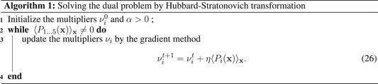
The algorithm is summarized as in Algorithm 1, where the braket notation ⟨⟩_x in Eq. 26 is the probabilistic summation of P(x), with the state of x sampled from the Hamiltonian H(x, ν) from Eq. 25 on the quantum annealing device or other optimization algorithm.

4 Experimental Results

In this section, we generate various problems with different settings in L_time, N_bus, N_pile based on realistic operational data of EV-buses. The continuous variables are discretized using N = 8 bit for binary encoding. We then analyze the experimental results on the minor embedding, directly sampling the QUBO model from the D-Wave-2000q quantum annealer, and the iterative method based on Hubbard-Stratonovich transformation. The ground truth optimal solution is obtained using the commercial solver Cplex. We also use the classical counterpart simulated annealing [48] as a benchmark.

4.1 Minor Embedding

First of all, we generate several instances of the EV-bus scheduling problem with different values of L_time, N_bus, N_pile based on real operational data. The problems are generated by randomly sampling from 15 typical bus operational schedules and randomly setting the number N_pile and power ω_j of charging piles in a reasonable range. We refer to Supplementary Figure S1 in the Supplementary Material for a visualization of these typical bus schedules.

To solve the problem via a quantum annealer, the logical problem (QUBO) graph needs first to be mapped to the hardware graph. In this case, the D-Wave-2000q has a Chimera architecture, which possesses a limited connectivity of degree 6. This implies that the number of physical qubits after the mapping is larger than the number of logical qubits in its original QUBO form, due to the minor embedding. We note that the minor embedding problem is NP-hard itself hence a heuristic algorithm is employed here [49]. Indeed, as analyzed in Section 2.4 and Section 3, the highly connected QUBO graph caused by the quadratic penalties increases significantly the number of qubits needed on the hardware to solve the EV-bus scheduling problem, even at a small scale.

The cost of embedding is illustrated in Figures 1A–D, where a problem with ∼ 150 qubits will cost ∼ 1,500 qubits on the hardware. We further observe a quadratic increase of physical qubits in Figure 1A when fixing N_bus = 1, N_pile = 1 and increasing L_time from 24 to 120, and a linear increase in Figures 1B–D where L_time is fixed. Consistently with the analysis in Section 2.3, we find thus that increasing the number of time steps L_time is more challenging in terms of hardware requirement than increasing N_bus, N_pile. This result further emphasizes that the extra qubits needed are mostly due to the quadratic penalty terms in $P_{\mathrm{3,4}}^2(\mathbf{x})={({\sum }_{j,k=1}^{D_{in}}{\omega }_j{x}_{ijk}+\dots )}^2$, where the number of variables x in the penalty increases with L_time.

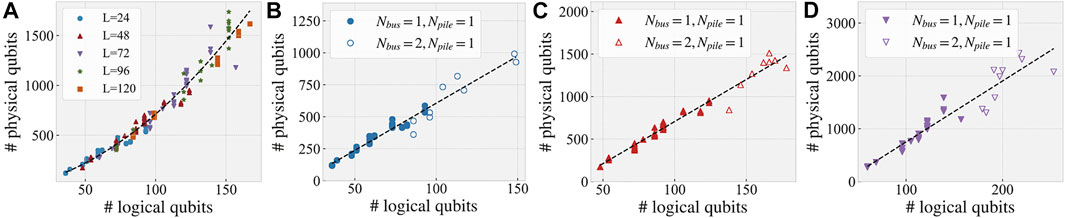
FIGURE 1. (A) The number of physical qubits needed to minor embed different problems, for fixed N_bus = 1, N_pile = 1 and L_time ∈ {24, 48, 72, 96, 120}. The dashed line is a quadratic regression fit. (B–D) Fixing L_time ∈{24, 48, 72}, and varying other problem parameters. N_bus, N_pile. The dashed lines are linear regression fits. The 16 × 16 Chimera graph from D-Wave 2000q sampler is used for all embeddings except for the large problems in (D), embedded onto a 24 × 24 Chimera graph.

4.2 Solving the Penalty Model

After minor embedding, the embedded problem is then sampled using the D-Wave quantum annealer as an efficient solver for QUBO problems. As discussed in Sections 2.3 and 2.4, the penalty coefficients λ_i for the penalties P_i need to be set appropriately to guarantee that the structure of the original problem is preserved. Additionally, the parameter J_{chain_strength} is introduced during minor-embedding to ensure that the physical qubits can be correctly mapped back to the logical qubits after the sampling. Although theoretical bounds, i.e., minimum theoretical values to ensure that the penalized optimal solution is the original one, are provided for λ_i in Section 2.3, in practice, the optimal values for P_i can not be directly calculated. Instead, we explore the trade-off between penalty and chain strength by computing the time to 99%-success, as defined in [14], and chain break fraction for an instance of the problem N_bus = 1, N_pile = 1, L_time = 24 solved with different settings of λ_3,4 and J_{chain_strength}. The coefficients λ_1,2 are constant to 10, since according to our previous results, these values are above their theoretical bounds and are of no significant effect on the efficiency of the solver.

As shown in Figure 2A, the time to 99%-success for this problem takes similar values along the lines J_{chain_strength} ∼ λ_3,4. However, this conclusion does not hold for other problems, as shown in Supplementary Figure S2 in the Supplementary Material, where the optimal λ_3,4 seems to be in the range [50, 800] for problems of larger sizes. We also observe that for λ_3,4 ≫ J_{chain_strength}, almost no solution could be found, which can be explained by an increased chain break fraction, as shown in Figure 2B. Equally for λ_3,4 ≪ J_{chain_strength}: although the quality of mapping is guaranteed by an increased chain strength, yet the efficiency of sampling by D-Wave QPUs is reduced. We conclude that choosing the optimal values for λ_3,4 and J_{chain_strength} is largely an empirical question that is problem dependent, but it is safer to set a penalty λ_3,4 close to the theoretical bounds and a chain strength J_{chain_strength} of the same order of magnitude as λ_3,4.

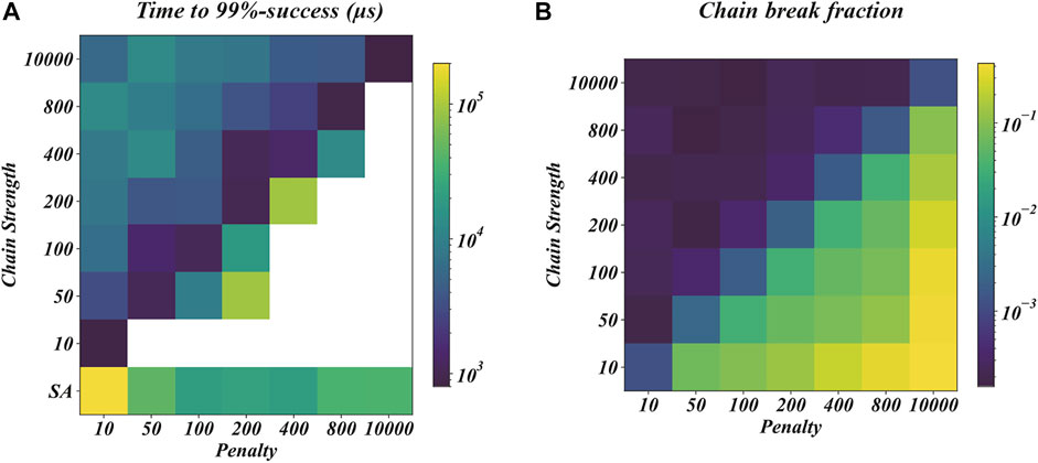
FIGURE 2. (A) Time to 99%-success in μs under different annealing parameters λ_3,4 (penalty coefficient) and J_{chain_strength} (chain strength for minor embedding) estimated based on 1,000 experiments on a problem with N_bus = 1, N_pile = 1, L_time = 24. White pixels indicate that no optimal solution has been found, “SA” label in the y-axis indicates solving the problem with simulated annealing. (B) Chain break fraction under the same experimental settings as in (A).

4.3 Solving With the Hubbard-Stratonovich Transformation

It is clear from the previous discussion that directly embedding and sampling the problem obtained with the penalty method suffers from several drawbacks and does not enable to solve large-scale problems. An alternative method discussed in Section 3 is proposed to obtain a better scaling with the quantum annealer. Using the Hubbard-Stratonovich transformation, the QUBO Hamiltonian H_QUBO(x) is transformed into an effective Hamiltonian H_QUBO(x, ν) with an additional multiplier ν. Then the remaining problem is to find the saddle point of the effective Hamiltonian, which is the original optimal solution. This method is similar to the Lagrangian dual method in classic optimization, and can reduce the quadratic terms into linear ones in the penalized QUBO energy.

To demonstrate the effectiveness of this method, we solve a bus charging scheduling problem with N_bus = 3, N_pile = 2 and L_time = 48. The QUBO formulation of this problem with quadratic penalty constraints could not be directly embedded onto the 16 × 16 Chimera graph of the D-Wave 2000q sampler. For reference, to embed such a problem onto a 24 × 24 Chimera graph would cost 2,499 physical qubits and the maximum chain length is 31. On the other hand, the dual Hamiltonian as defined in Eq. 25 only requires 320 physical qubits to embed with a maximum chain length of 4. This example illustrates thus clearly that the limitation for connectivity is well mitigated after the Hubbard-Stratonovich transformation.

We investigate then whether the iterative approach can lead to the ground state of the original Hamiltonian, i.e., the optimal schedule with minimum cost and satisfying all constraints. As shown in Figures 3A,B, the optimal solution is obtained after 96 iterations of updating the multipliers ν based on the sampling of the dual Hamiltonian with the D-Wave 2000q annealer. In Figure 3A, we visualize the state-of-charge SOC of the optimal solutions found while sampling the dual Hamiltonian at different iterations. It can be seen that while updating the multipliers ν according to Algorithm 1, the state of charge gradually falls into the interval [0.3, 1], where the constraints are satisfied. Figure 3B displays the distribution of different samples returned by both the D-Wave 2000q annealer and simulated annealing. We note that the multipliers ν are updated according to the lowest energy samples returned by D-Wave’s machine. We observe that the sampled lowest energy of the dual Hamiltonian does not decrease monotonically. This might be caused by multiple reasons. Firstly, the sampling, quantum or classical, is a heuristic process so that the actual ground states of the dual Hamiltonian are not necessarily found at each iteration, as shown in Figure 3B. Secondly, the energy landscape of the dual Hamiltonian might be non-convex, as also discussed by Ohzeki when this method is proposed [32]. Thirdly, the learning rate might be too large.

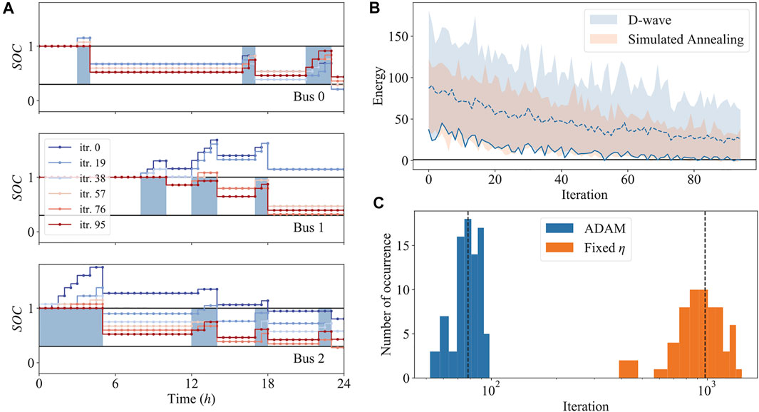
FIGURE 3. (A) State-of-charge SOC at different iterations calculated based on the lowest energy sample from D-Wave annealer with the Hubbard-Stratonovich (HS) transformation method. The two solid black lines indicate respectively SOC = 0.3 and SOC = 1, between which the constraints are satisfied. Blue shaded areas represent the time intervals during which the bus is available for charging. (B) Distribution of the sampled energy of the dual Hamiltonian at each iteration. The blue and orange shaded areas represent sampling results from the D-Wave sampler and simulated annealing, respectively. The blue solid (respectively, dashed) line indicates the lowest value (respectively, the median) of the samples. The black solid line marks the lowest energy of the original Hamiltonian (without HS transformation) sampled by simulated annealing with an extended period of time. (C) Histogram of number of iterations till convergence (all constraints are satisfied) with two different strategies of updating the multipliers μ: ADAM represents adaptive gradient and constant learning rate η = 0.1. All plots are obtained for the same problem with parameters N_bus = 3, N_pile = 2, L_time = 48.

From an optimization perspective, the aforementioned three points imply that in practice, the task of solving for the multipliers ν is carried out in a complex landscape with noisy evaluations of the gradient. In this context, finding the optimal multipliers, hence the saddle point could be very challenging, especially with a large number of multipliers. To resolve this problem, instead of using a fixed learning rate η = 0.1, we have employed an adaptive gradient method to update the multipliers ν, with ADAM solver for stochastic optimization [50]. To further confirm the effectiveness of the adaptive gradient methods, we have solved the problem multiple times with the two different strategies, ADAM or fixed learning rate. It is observed in Figure 3C that the adaptive gradient approach for updating ν has a significant advantage over fixing the learning rate, requiring about 10 times less iterations to converge. This emphasizes thus that the practical constraint caused by the transformation, namely performing a classical gradient descent, requires careful tuning in order to reduce the additional computational overhead, which ADAM achieves. Yet, we note that it has been proven that ADAM as described in [50] could possibly diverge, even in the convex case [51]. Hence, the convergence of ADAM-type methods has been analyzed theoretically in several recent contributions. For instance, Chen et al. derive a set of sufficient conditions to guarantee the convergence of AmsGrad, a variant of Adam, with a rate of $O\left(\frac{\log T+d^2}{\sqrt{T}}\right)$ for non-convex stochastic optimization [52], where T is the number of iterations of the algorithm and d the dimension of the problem. Similarly, Zhou et al. achieve a rate of $O(\sqrt{d/T}+d/T)$ for AmsGrad [53]. The interested reader is also referred to [54–57] for more in-depth analyses of adaptive gradient algorithms. Consequently, although ADAM has shown to be an appropriate choice for solving the bus charging scheduling problem, further work could explore the impact of the adaptive gradient method on the convergence and computational cost of this iterative approach.

5 Conclusion

In this work, we have solved a realistic EV-bus charging scheduling problem with D-Wave’s quantum annealer. Firstly, we have reformulated the original integer optimization problem with inequality constraints into a QUBO problem by the penalty method. Furthermore, theoretical analysis on the lower bound of the penalty and experimentation with minor embedding emphasize the fact that the key challenge for quantum annealing to solve the bus charging scheduling problem is two-fold: on one hand, the number of additional qubits needed for minor embedding and on the other hand, the penalty bounds to preserve the structure of the original problem. We analyze these problems with numerical experiments and find out that the former problem is caused by the quadratic penalty which makes it especially difficult to increase the number of time steps when modeling the problem. The latter challenge is linked to the case-dependent problem structure and the dynamic range of the physical device, which have a joint effect on the efficiency of quantum annealing.

To mitigate the above problems, we have employed an iterative approach based on the Hubbard-Stratonovich transformation proposed by Ohzeki [32]. This method reduces the quadratic penalty terms in the original QUBO Hamiltonian into linear terms in its dual Hamiltonian with the Hubbard-Stratonovich transformation. Then by iteratively solving the dual Hamiltonian to update the multipliers ν introduced by the transformation, the ground state of the original QUBO Hamiltonian, hence the optimal solution of the original problem, can be found. We demonstrated that it is possible to solve a larger-scale problem which can not be directly embedded onto the D-Wave 2000q′s Chimera graph with this approach. Besides, we observed that due to the noisy gradient evaluation caused by the heuristic sampling process and the complex energy landscape, it is significantly more efficient to update the multipliers in an adaptive manner, for instance with ADAM solver, instead of using a fixed learning rate.

As believed by many, quantum annealing can provide speedup for certain optimization problems with quantum tunneling effect. However in practice, the physical implementation for a quantum annealer contains only two-body and mostly neighbouring interactions between qubits (spins). This means that the ideal problems for a physical quantum annealer to solve in the near future are limited to problems which can be formulated as QUBO problems on a sparsely connected graph. While a large portion of the optimization problems can be eventually reformulated as QUBOs by encoding continuous variables, introducing penalties and ancillary qubits, it will generally induce an additional burden in terms of connectivity and dynamic range of the physical device. The Hubbard-Stratonovich transformation can be a possible way of alleviating this cost and solving larger-scale problems with an iterative procedure. Under the Hubbard-Stratonovich transformation, the complexity of solving the original problem is transformed into both solving the dual problem and the optimization of the multipliers, where the latter can be achieved using a classical computer. In this sense, this approach can be considered as a hybrid classical-quantum algorithm where the advantage of the quantum computing is better utilized. We believe that similar to the EV-bus charging scheduling problem considered in this work, many more realistic use-cases can be better solved by quantum annealing with the combination of Hubbard-Stratonovich transformation and adaptive gradient descent.

Data Availability Statement

The datasets presented in this article are not readily available because Bus electrical consumption is a proprietary data shared by a third party entity. Requests to access the datasets should be directed to TN, tahar.nabil@edf.fr.

Author Contributions

All authors listed have made a substantial, direct, and intellectual contribution to the work and approved it for publication.

Conflict of Interest

SY and TN were employed by EDF R&D China Center.

Publisher’s Note

All claims expressed in this article are solely those of the authors and do not necessarily represent those of their affiliated organizations, or those of the publisher, the editors and the reviewers. Any product that may be evaluated in this article, or claim that may be made by its manufacturer, is not guaranteed or endorsed by the publisher.

Acknowledgments

The authors thank EDF Group for supporting such exploratory research projects as well as Marc Porcheron and Bingqian Liu from EDF R&D for comments on the manuscript and useful discussions. We also thank D-Wave’s team, in particular Andy Mason, for providing easy access to the Quantum Processing Units.

Supplementary Material

The Supplementary Material for this article can be found online at: https://www.frontiersin.org/articles/10.3389/fphy.2021.730685/full#supplementary-material

References

1. Feynman RP Simulating Physics with Computers. Int J Theor Phys (1982) 21:467–88. doi:10.1007/BF02650179
2. Shor PW Algorithms for Quantum Computation: Discrete Logarithms and Factoring. In: Proceedings 35th annual symposium on foundations of computer science; Singer Island, FL. IEEE (1994). p. 124–34.
3. Lloyd S Universal Quantum Simulators. Science (1996) 273:1073–8. doi:10.1126/science.273.5278.1073
4. Berry DW, Childs AM, Cleve R, Kothari R, Somma RD Exponential Improvement in Precision for Simulating Sparse Hamiltonians. In: Proceedings of the forty-sixth annual ACM symposium on Theory of computing; New York, NY (2014) p. 283–92. STOC ’14. doi:10.1145/2591796.2591854
5. Grover LK A Fast Quantum Mechanical Algorithm for Database Search. In: Proceedings of the twenty-eighth annual ACM symposium on Theory of computing; Philadelphia, PA (1996) p. 212–9. doi:10.1145/237814.237866
6. Arute F, Arya K, Babbush R, Bacon D, Bardin JC, Barends R, et al. Quantum Supremacy Using a Programmable Superconducting Processor. Nature (2019) 574:505–10. doi:10.1038/s41586-019-1666-5
7. Zhong HS, Wang H, Deng YH, Chen MC, Peng LC, Luo YH, et al. Quantum Computational Advantage Using Photons. Science (2020) 370. 1460, 3. doi:10.1126/science.abe8770
8. Kadowaki T, Nishimori H Quantum Annealing in the Transverse Ising Model. Phys Rev E (1998) 58:5355–63. doi:10.1103/PhysRevE.58.5355
9. Brooke J, Bitko D, Aeppli G Quantum Annealing of a Disordered Magnet. Science (1999) 284:779–81. doi:10.1126/science.284.5415.779
10. Farhi E, Goldstone J, Gutmann S, Lapan J, Lundgren A, Preda D A Quantum Adiabatic Evolution Algorithm Applied to Random Instances of an NP-Complete Problem. Science (2001) 292:472–5. doi:10.1126/science.1057726
11. Santoro GE, Martoňák R, Tosatti E, Car R Theory of Quantum Annealing of an Ising Spin Glass. Science (2002) 295:2427–30. doi:10.1126/science.1068774
12. Marshall J, Venturelli D, Hen I, Rieffel EG Power of Pausing: Advancing Understanding of Thermalization in Experimental Quantum Annealers. Phys Rev Appl (2019) 11:044083. doi:10.1103/PhysRevApplied.11.044083
13. Chancellor N An Overview of Approaches to Modernize Quantum Annealing Using Local Searches. Electron Proc Theor Comput Sci (2016) 214:16–21. doi:10.4204/EPTCS.214.4
14. Ronnow TF, Wang Z, Job J, Boixo S, Isakov SV, Wecker D, et al. Defining and Detecting Quantum Speedup. Science (2014) 345:420–4. doi:10.1126/science.1252319
15. Boixo S, Rønnow TF, Isakov SV, Wang Z, Wecker D, Lidar DA, et al. Evidence for Quantum Annealing with More Than One Hundred Qubits. Nat Phys (2014) 10:218–24. doi:10.1038/nphys2900
16. Hen I, Job J, Albash T, Rønnow TF, Troyer M, Lidar DA Probing for Quantum Speedup in Spin-Glass Problems with Planted Solutions. Phys Rev A (2015) 92:042325. doi:10.1103/PhysRevA.92.042325
17. Denchev VS, Boixo S, Isakov SV, Ding N, Babbush R, Smelyanskiy V, et al. What Is the Computational Value of Finite-Range Tunneling? Phys Rev X (2016) 6:1–17. doi:10.1103/PhysRevX.6.031015
18. Mandrà S, Zhu Z, Wang W, Perdomo-Ortiz A, Katzgraber HG Strengths and Weaknesses of Weak-strong Cluster Problems: A Detailed Overview of State-Of-The-Art Classical Heuristics versus Quantum Approaches. Phys Rev A (2016) 94:022337. doi:10.1103/PhysRevA.94.022337
19. Rieffel EG, Venturelli D, O’Gorman B, Do MB, Prystay EM, Smelyanskiy VN A Case Study in Programming a Quantum Annealer for Hard Operational Planning Problems. Quan Inf Process (2015) 14:1–36. doi:10.1007/s11128-014-0892-x
20. Venturelli D, Marchand DJ, Rojo G Job-shop Scheduling Solver Based on Quantum Annealing. In: Proceedings of the 11th Workshop on Constraint Satisfaction Techniques for Planning and Scheduling Problems; London, United Kingdom (2016). COPLAS 2016.
21. Tran TT, Do M, Rieffel EG, Frank J, Wang Z, O’Gorman B, et al. A Hybrid Quantum-Classical Approach to Solving Scheduling Problems. In: Proceedings of the 9th Annual Symposium on Combinatorial Search; Tarrytown, NY (2016). p. 98–106. SoCS 2016.
22. Adachi SH, Henderson MP Application of Quantum Annealing to Training of Deep Neural Networks. arXiv (2015). arXiv:1510.06356. Available from: https://arxiv.org/abs/1510.06356.
23. Amin MH, Andriyash E, Rolfe J, Kulchytskyy B, Melko R Quantum Boltzmann Machine. Phys Rev X (2018) 8:021050. doi:10.1103/PhysRevX.8.021050
24. Perdomo-Ortiz A, Dickson N, Drew-Brook M, Rose G, Aspuru-Guzik A Finding Low-Energy Conformations of Lattice Protein Models by Quantum Annealing. Sci Rep (2012) 2:571. doi:10.1038/srep00571
25. Hernandez M, Aramon M Enhancing Quantum Annealing Performance for the Molecular Similarity Problem. Quan Inf Process (2017) 16:133. doi:10.1007/s11128-017-1586-y
26. Rosenberg G, Haghnegahdar P, Goddard P, Carr P, Wu K, De Prado ML Solving the Optimal Trading Trajectory Problem Using a Quantum Annealer. IEEE J Sel Top Signal Process (2016) 10:1053–60. doi:10.1109/JSTSP.2016.2574703
27. Venturelli D, Kondratyev A Reverse Quantum Annealing Approach to Portfolio Optimization Problems. Quan Mach. Intell. (2019) 1:17–30. doi:10.1007/s42484-019-00001-w
28. Mehta A, Muradi M, Woldetsadick S Quantum Annealing Based Optimization of Robotic Movement in Manufacturing. In: International Workshop on Quantum Technology and Optimization Problems. Munich, Germany: Springer (2019) p. 136–44. doi:10.1007/978-3-030-14082-3_12
29. Neukart F, Compostella G, Seidel C, Von Dollen D, Yarkoni S, Parney B Traffic Flow Optimization Using a Quantum Annealer. Front ICT (2017) 4:29. doi:10.3389/fict.2017.00029
30. Ajagekar A, You F Quantum Computing for Energy Systems Optimization: Challenges and Opportunities. Energy (2019) 179:76–89. doi:10.1016/j.energy.2019.04.186
31. Lucas A Ising Formulations of many NP Problems. Front Phys (2014) 2:1–14. doi:10.3389/fphy.2014.00005
32. Ohzeki M Breaking Limitation of Quantum Annealer in Solving Optimization Problems under Constraints. Sci Rep 10 (2020) 1–12. doi:10.1038/s41598-020-60022-5
33. Glover F, Kochenberger G, Du Y Quantum Bridge Analytics I: a Tutorial on Formulating and Using QUBO Models. 4or-q J Oper Res (2019) 17:335–71. doi:10.1007/s10288-019-00424-y
34. Tamura N, Taga A, Kitagawa S, Banbara M Compiling Finite Linear CSP into SAT. Constraints (2009) 14:254–72. doi:10.1007/s10601-008-9061-0
35. Fiacco AV, McCormick GP Nonlinear Programming: Sequential Unconstrained Minimization Techniques. Philadelphia: SIAM (1990).
36. D-Wave Systems Inc D-wave System Documentation (2021). Available at: https://docs.dwavesys.com/docs/latest/c_qpu_1.html (Accessed June 24, 2021).
37. Boothby K, Bunyk P, Raymond J, Roy A Next-Generation Topology of D-Wave Quantum Processors. arXiv (2020). arXiv:2003.00133. Available from: https://arxiv.org/abs/2003.00133.
38. Choi V Minor-embedding in Adiabatic Quantum Computation: I. The Parameter Setting Problem. Quan Inf Process (2008) 7:193–209. doi:10.1007/s11128-008-0082-9
39. Choi V Minor-embedding in Adiabatic Quantum Computation: II. Minor-Universal Graph Design. Quan Inf Process (2011) 10:343–53. doi:10.1007/s11128-010-0200-3
40. Fang Y-L, Warburton PA Minimizing Minor Embedding Energy: an Application in Quantum Annealing. Quan Inf Process (2020) 19:191. doi:10.1007/s11128-020-02681-x
41. Hen I, Sarandy MS Driver Hamiltonians for Constrained Optimization in Quantum Annealing. Phys Rev A (2016) 93:062312. doi:10.1103/PhysRevA.93.062312
42. Hen I, Spedalieri FM Quantum Annealing for Constrained Optimization. Phys Rev Appl (2016) 5:034007. doi:10.1103/PhysRevApplied.5.034007
43. Vyskocil T, Djidjev H Embedding equality Constraints of Optimization Problems into a Quantum Annealer. Algorithms (2019) 12:77–24. doi:10.3390/A12040077
44. Vyskočil T, Pakin S, Djidjev HN Embedding Inequality Constraints for Quantum Annealing Optimization. In: S Feld, and C Linnhoff-Popien, editors. Quantum Technology and Optimization Problems. Munich, Germany: Springer International Publishing (2019) p. 11–22. doi:10.1007/978-3-030-14082-3_2
45. Ajagekar A, Humble T, You F Quantum Computing Based Hybrid Solution Strategies for Large-Scale Discrete-Continuous Optimization Problems. Comput Chem Eng (2020) 132:106630–50. doi:10.1016/j.compchemeng.2019.106630
46. Hubbard J Calculation of Partition Functions. Phys Rev Lett (1959) 3:77–8. doi:10.1103/PhysRevLett.3.77
47. Stratonovich RL On a Method of Calculating Quantum Distribution Functions. Soviet Phys Doklady (1957) 2:416.
48. Van Laarhoven PJM, Aarts EHL Simulated Annealing. In: Simulated Annealing: Theory and Applications. Dordrecht: Springer (1987) p. 7–15. doi:10.1007/978-94-015-7744-1_2
49. Cai J, Macready WG, Roy A A Practical Heuristic for Finding Graph Minors. arXiv (2014). arXiv:1406.2741. Available from: https://arxiv.org/abs/1406.2741.
50. Kingma DP, Ba J Adam: A Method for Stochastic Optimization. In: 3rd International Conference on Learning Representations; San Diego, CA (2015).
51. Reddi SJ, Kale S, Kumar S On the Convergence of Adam and Beyond. In: 6th International Conference on Learning Representations; Vancouver, Canada (2018).
52. Chen X, Liu S, Sun R, Hong M On the Convergence of a Class of Adam-type Algorithms for Non-convex Optimization. In: 7th International Conference on Learning Representations; New Orleans, LA (2019).
53. Zhou D, Chen J, Cao Y, Tang Y, Yang Z, Gu Q On the Convergence of Adaptive Gradient Methods for Nonconvex Optimization. arXiv (2018). arXiv:1808.05671. Available from: https://arxiv.org/abs/1808.05671.
54. Basu A, De S, Mukherjee A, Ullah E Convergence Guarantees for RMSProp and ADAM in Non-Convex Optimization and Their Comparison to Nesterov Acceleration on Autoencoders. In: ICML Workshop on Modern Trends in Nonconvex Optimization for Machine Learning; Stockholm, Sweden (2018).
55. Zou F, Shen L, Jie Z, Zhang W, Liu W A Sufficient Condition for Convergences of Adam and RMSProp. In: Proceedings of the IEEE/CVF Conference on Computer Vision and Pattern Recognition; Long Beach, CA (2019). p. 11119–27. doi:10.1109/CVPR.2019.01138
56. Luo L, Xiong Y, Liu Y, Sun X Adaptive Gradient Methods with Dynamic Bound of Learning Rate. In: 7th International Conference on Learning Representations; New Orleans, LA (2019). Available from: https://openreview.net/forum?id=Bkg3g2R9FX.
57. Barakat A, Bianchi P Convergence Analysis of a Momentum Algorithm with Adaptive Step Size for Non Convex Optimization. arXiv (2019). arXiv:1911.07596. Available from: https://arxiv.org/abs/1911.07596.
Keywords: optimization, quantum annealing, hubbard-stratonovich transformation, integer programing, scheduling problem, quantum applications
Citation: Yu S and Nabil T (2021) Applying the Hubbard-Stratonovich Transformation to Solve Scheduling Problems Under Inequality Constraints With Quantum Annealing. Front. Phys. 9:730685. doi: 10.3389/fphy.2021.730685
Received: 25 June 2021; Accepted: 26 August 2021;
Published: 14 September 2021.
Edited by:
Alexandre M. Souza, Centro Brasileiro de Pesquisas Físicas, BrazilReviewed by:
Celso Villas-Boas, Federal University of Sao Carlos, BrazilEduardo Inacio Duzzioni, Federal University of Santa Catarina, Brazil
Copyright © 2021 Yu and Nabil. This is an open-access article distributed under the terms of the Creative Commons Attribution License (CC BY). The use, distribution or reproduction in other forums is permitted, provided the original author(s) and the copyright owner(s) are credited and that the original publication in this journal is cited, in accordance with accepted academic practice. No use, distribution or reproduction is permitted which does not comply with these terms.
*Correspondence: Sizhuo Yu, yusizhuo@buaa.edu.cn; Tahar Nabil, tahar.nabil@edf.fr