
W-band MIMO GB-SAR for Bridge Testing/Monitoring


Department of Information Engineering, University of Florence, Via di Santa Marta 3, 350139 Firenze, Italy
*
Author to whom correspondence should be addressed.
Electronics 2021, 10(18), 2261; https://doi.org/10.3390/electronics10182261
Submission received: 27 August 2021
/
Revised: 10 September 2021
/
Accepted: 13 September 2021
/
Published: 14 September 2021
(This article belongs to the Special Issue Intelligent Radar Platform Technology for Smart Environments)
Abstract
:Interferometric radars are widely used for static and dynamic monitoring of large structures such as bridges, culverts, wind turbine towers, chimneys, masonry towers, stay cables, buildings, and monuments. Most of these radars operate in Ku-band (17 GHz). Nevertheless, a higher operative frequency could allow the design of smaller, lighter, and faster equipment. In this paper, a fast MIMO-GBSAR (Multiple-Input Multiple-Output Ground-Based Synthetic Aperture Radar) operating in W-band (77 GHz) has been proposed. The radar can complete a scan in less than 8 s. Furthermore, as its overall dimension is smaller than 230 mm, it can be easily fixed to the head of a camera tripod, which makes its deployment in the field very easy, even by a single operator. The performance of this radar was tested in a controlled environment and in a realistic case study.
1. Introduction
Bridges require testing before going into service and need to be periodically monitored during their operative life for evaluating possible damage. Both testing and monitoring can be performed by static and dynamic measurements. The static test of a bridge is carried out by loading the deck with a dead load of several tons, and dynamic measurements are aimed at evaluating the response of the bridge stimulated by dynamic loads such as mechanical impulses, vibrodynes, and vehicular traffic.
Interferometric radars can perform both tests [1] operating in the real-aperture modality [2,3,4] or synthetic aperture modality [5,6]. The latter is usually called GB-SAR (Ground-Based Synthetic Aperture Radar).
Drawbacks of the current GB-SAR systems for structural monitoring are the slow acquisition rate (up to 90 s), physical dimensions (2–3 m) and weight (50–100 kg), which could preclude installation in many operative scenarios.
In order to reduce the acquisition time, MIMO (Multiple-Input Multiple-Output) systems have been proposed for bridge monitoring [7,8] and for environmental monitoring [9,10]. The MIMO radar reduces the acquisition time but dramatically increases hardware cost and complexity.
A way to reduce the size of a GB-SAR is operating at a higher frequency; for example, in W-band (77 GHz) instead of Ku-band (17 GHz). Radars operating in W-band have been proposed for different applications, especially in the automotive field [11,12,13,14]. These radars are characterized by small dimensions (often they are installed inside the headlight of a car) and by a fast repetition rate (up to 1500 Hz).
The first interferometric ArcSAR (circular synthetic aperture) operating in W-band was presented in 2018 [15,16,17,18,19] by IDS Georadar, Pisa, Italy. This sensor, named HYDRA, operates at 77 GHz and performs a scan with a minimum time of 30 s. The sensor is able to co-register a radar image with a three-dimensional lidar scanner. The radar acquisition is projected on the 3D surface and the sensor can provide the displacement information of a 3D volume.
In this paper, the authors present a fast and small GB-SAR operating at 77 GHz based on a multiple MIMO radar. The MIMO antennas are positioned orthogonally with respect to the linear rail (or actuator) and the radar moves at constant speed along the guide. The azimuth resolution is provided by the movement along the linear rail, while the elevation resolution is provided by the MIMO architecture. The GB-SAR operates on-the-fly acquisition [20] for increasing the acquisition speed, reducing the blurring due to moving targets, and for increasing the duty cycle (the ratio between the total acquisition time and the repetition time during a measurement cycle). The radar is able to scan the scene in less than 8 s (which is the mechanic limit of the used actuator).
The main novelty of the proposed radar, with respect to the scientific literature (e.g., [15,16]) is the scan time of the order of a few seconds obtained by combining on-the-fly acquisition and MIMO architecture for elevation resolution. This feature opens many practical applications that are precluded by slower radar systems.
2. Materials and Methods
2.1. The Radar Protype
The MIMO-GBSAR reported in this article is based on the AWR1843BOOST [21] by Texas Instruments. The radar is a MIMO that provides a Continuous Wave Frequency Modulated (FMCW) signal.
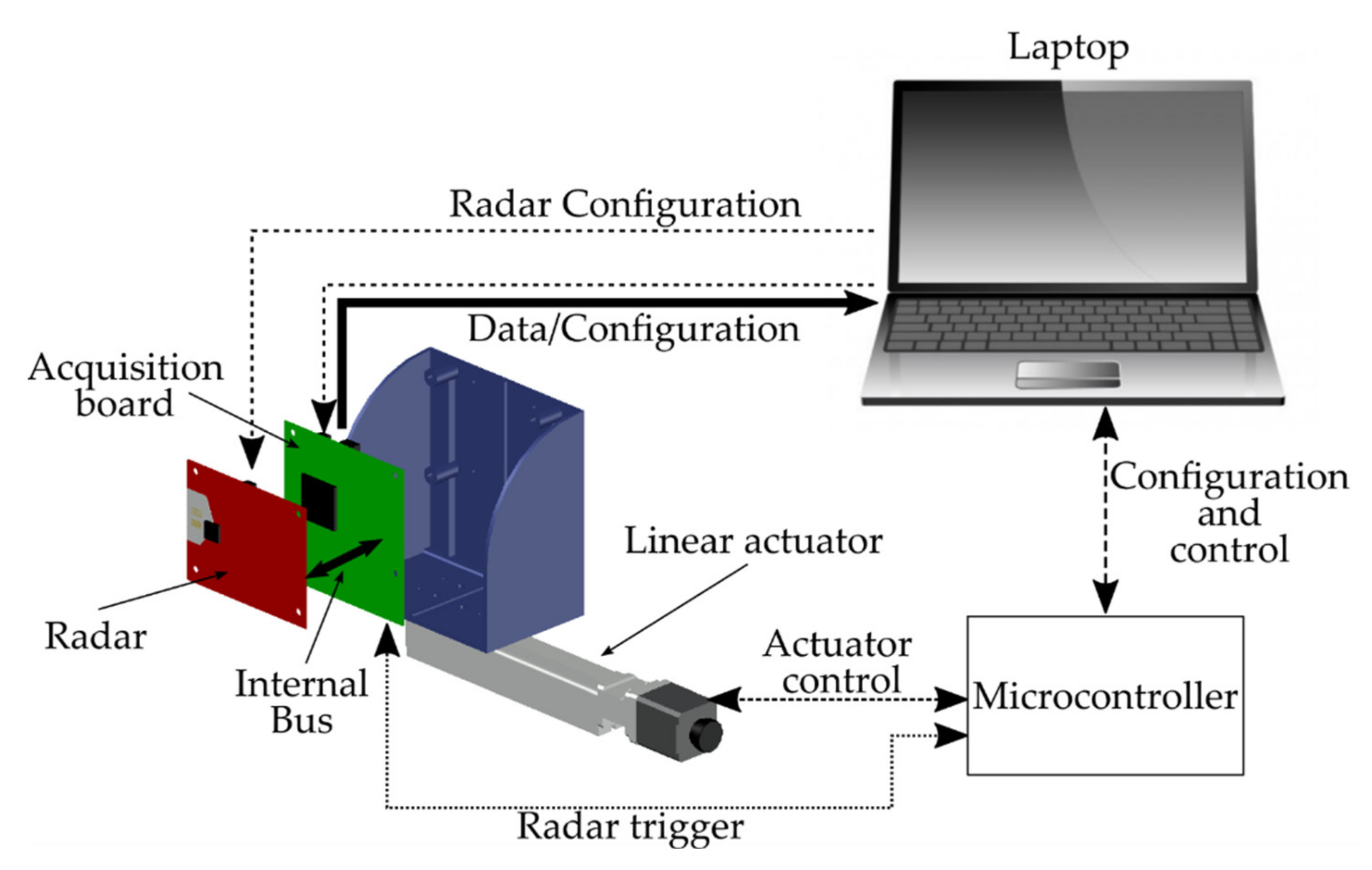
Figure 1 shows a sketch of the GB-SAR prototype. The radar is connected to an acquisition board (DCA1000EVM by Texas Instruments, Dallas, TX, USA). The acquisition board ensures the transfer of RAW data to the laptop. The radar and the acquisition board are fixed on a linear actuator.
A microcontroller provides the trigger to the radar and controls the movement of the actuator.
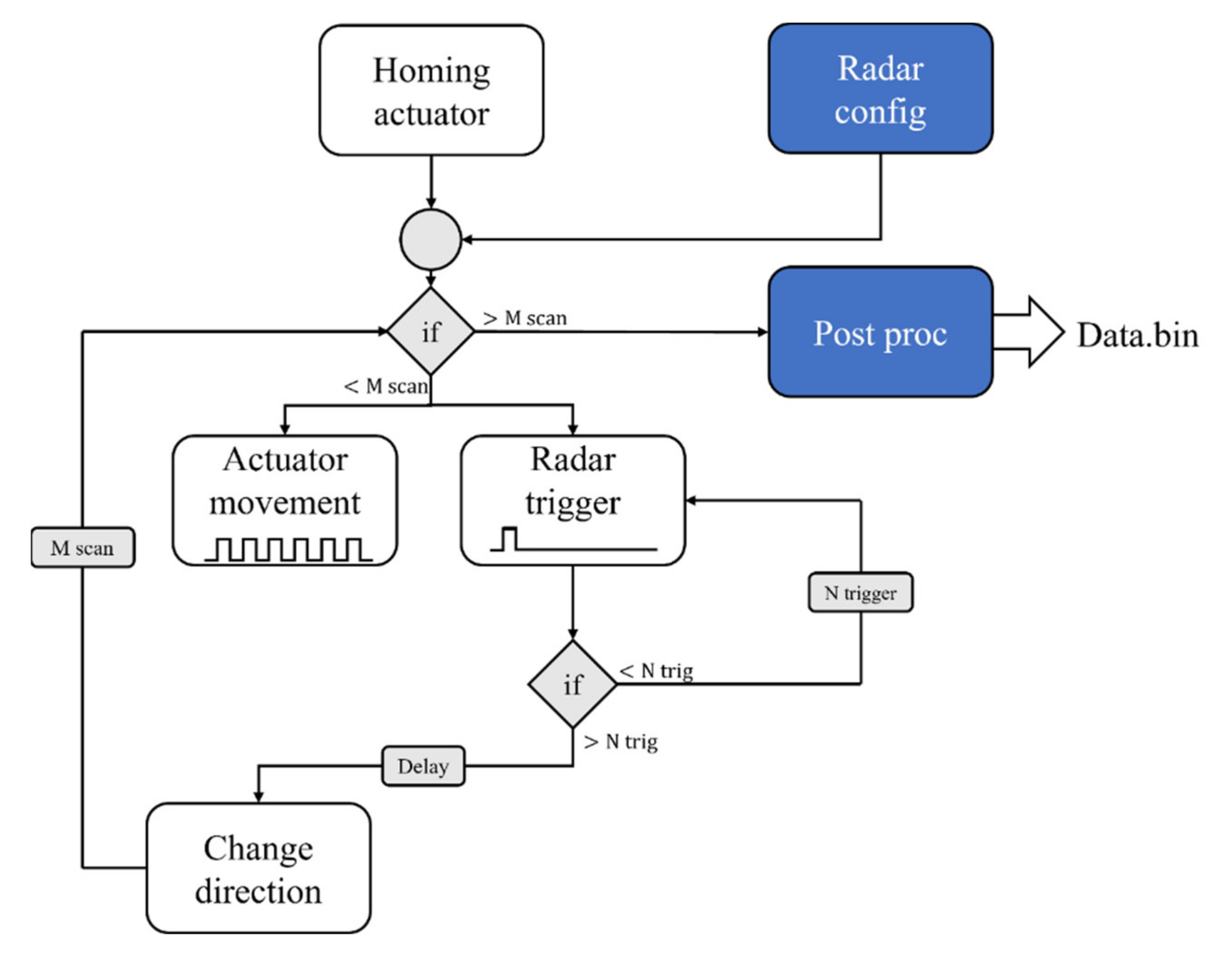
The microcontroller manages the movement of the actuator and the trigger of the radar (the white block in Figure 2). When the preliminary configuration has been set (Radar config and Homing actuator), the microcontroller generates N trigger to the radar and moves the actuator for performing a scan.
After N trigger, the microcontroller changes the actuator direction and the system performs a reverse scan. Indeed, this radar can perform the acquisition in both scan directions (from right to left and vice versa). This feature increases the measurement duty cycle.
The radar configuration and the data acquisition were performed by software provided by Texas Instruments [22] (the blue blocks in Figure 2). When all the scans are acquired (M scans), a post-processing routine generates a binary file from RAW data by zero padding the possible missing data. Indeed, the protocol between the radar and acquisition board is the User Datagram Protocol (UDP).
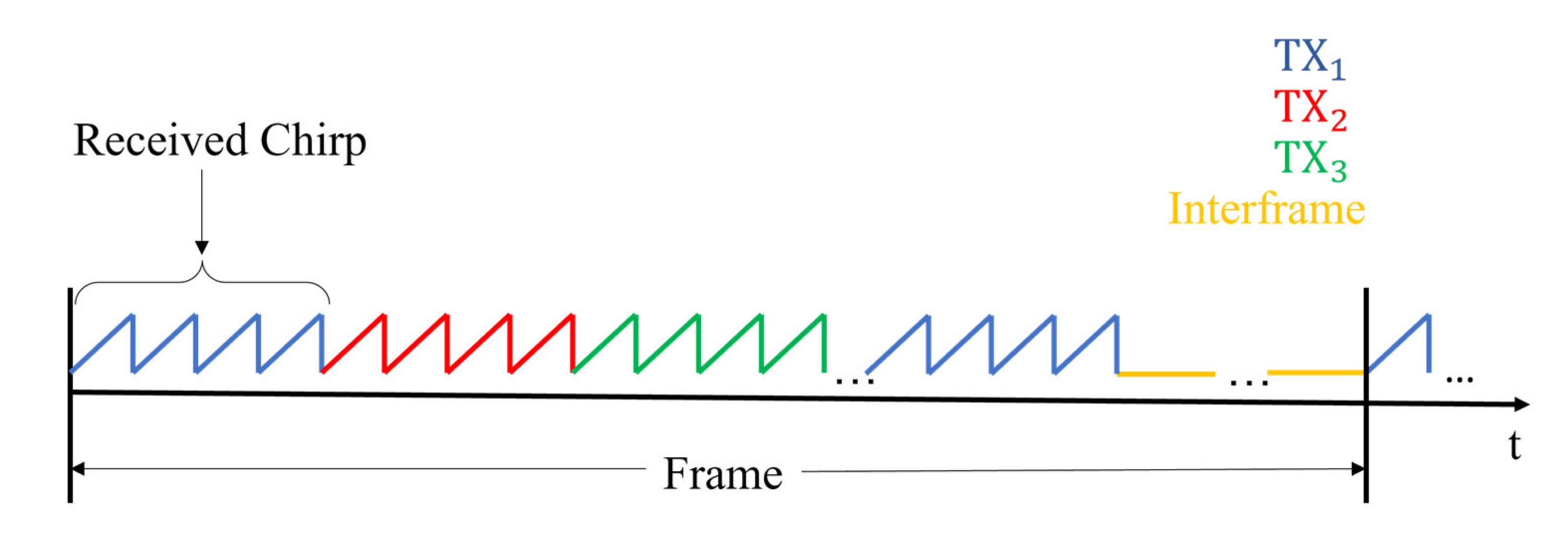
AWR1843 was designed for automotive purposes. The operation of this radar is shown in Figure 3: a frequency sweep, called a chirp, is transmitted by the three TX antennas sequentially. The back-scattered signal is received simultaneously by the four RX antennas. The chirps are grouped in a structure called a frame. The numbers of the chirps can be selected, and this depends on the kind of application. The radar can perform preprocessing analysis (e.g., target detection in obstacle avoidance applications) in the time between two frames. In this specific implementation, the interframe time has been reduced to its minimum, as the data are processed after an entire acquisition. Each frame can be triggered by the microcontroller (Figure 2) or by the acquisition software.
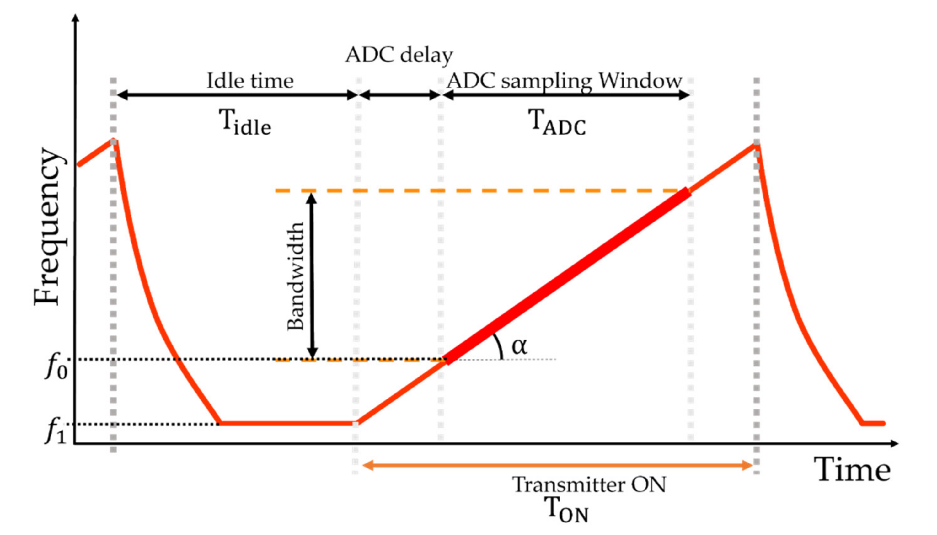
Figure 4 shows an example of a chirp. The signal is transmitted during the period named and it is acquired by a digital converter within the “ADC sampling Window”; finally, it is saved on the acquisition board.
The duration of the “ADC sampling Window” depends on the frequency of the digital converter () and on the number of ADC samples (). After the period T_ON, the transmitting channels are switched off for a time equal to .
The unambiguous range of the radar is given by [23]:
with c as the speed of light and α as the frequency slope.
The bandwidth is given by:
with .
The radar provides up to 2 GHz of bandwidth from to and from to . The maximum ADC sample is 4096 and the typical acquisition frequency is 10.00 MHz. The transmitting power is 0 dBm and the receiving gain is . The antenna gain is .
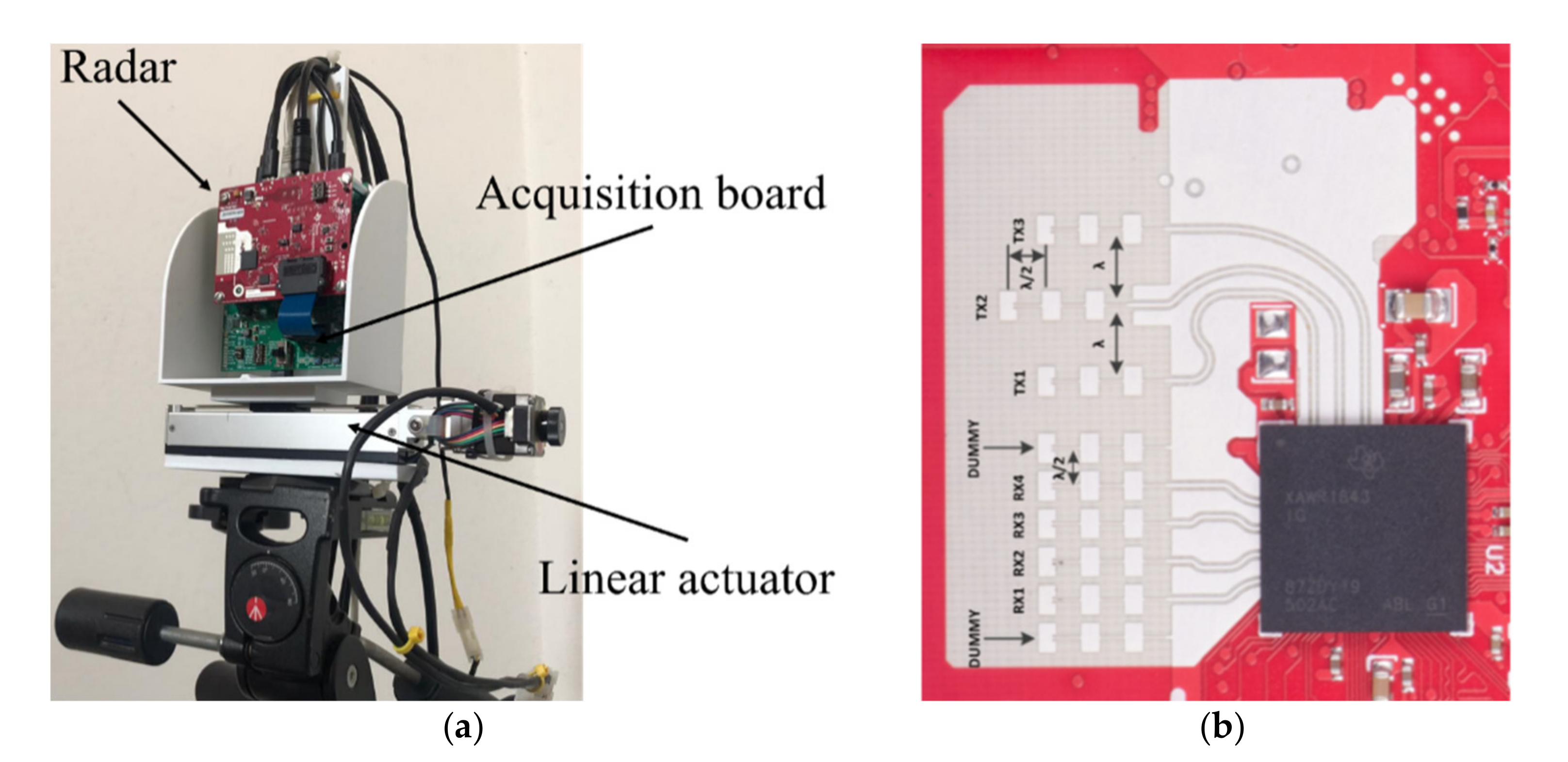
A picture of the GB-SAR prototype is shown in Figure 5. The scan length is 63.50 mm for an azimuth resolution of 1.75°. This resolution corresponds to ∼300 mm of scan at 17 GHz ().
The elevation resolution, given by the MIMO (Figure 5b), is about 10°. Indeed, the virtual antennas are arranged with a step of .
The GB-SAR completes a single scan in about with a duty cycle of about (). The scan time is limited by the maximum speed of the actuator.
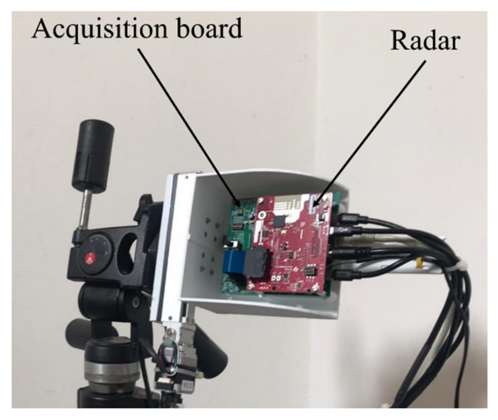
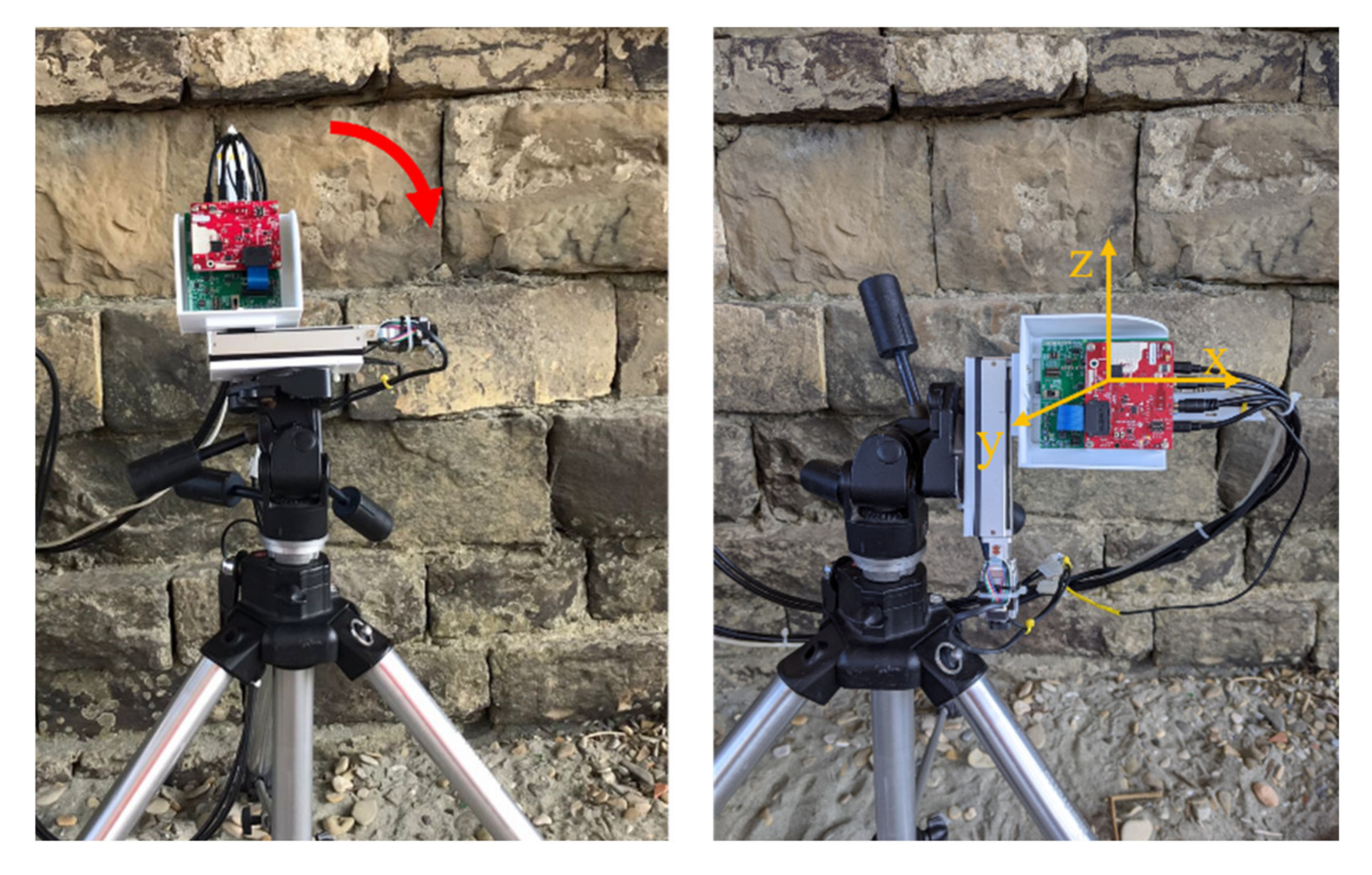
The radar prototype can operate in two modalities: the MIMO-SAR modality and the only-MIMO modality. The MIMO-SAR modality allows a high resolution in range and azimuth but poor resolution in elevation. In this modality, the scan interval is of the order of seconds and can be used for the static monitoring of bridges. The same radar operating in the only-MIMO modality can be used in the dynamic monitoring of bridges. Indeed, by rotating the radar 90° along the y axis (Figure 6) and by stopping the mechanical linear actuator, the MIMO radar can sample the environment with a high repetition rate (more than 500 Hz) [24,25]. The azimuth resolution is given by the MIMO antennas, and it is about 10°. In this operative modality, the trigger is provided by the acquisition software.
2.2. Data Processing
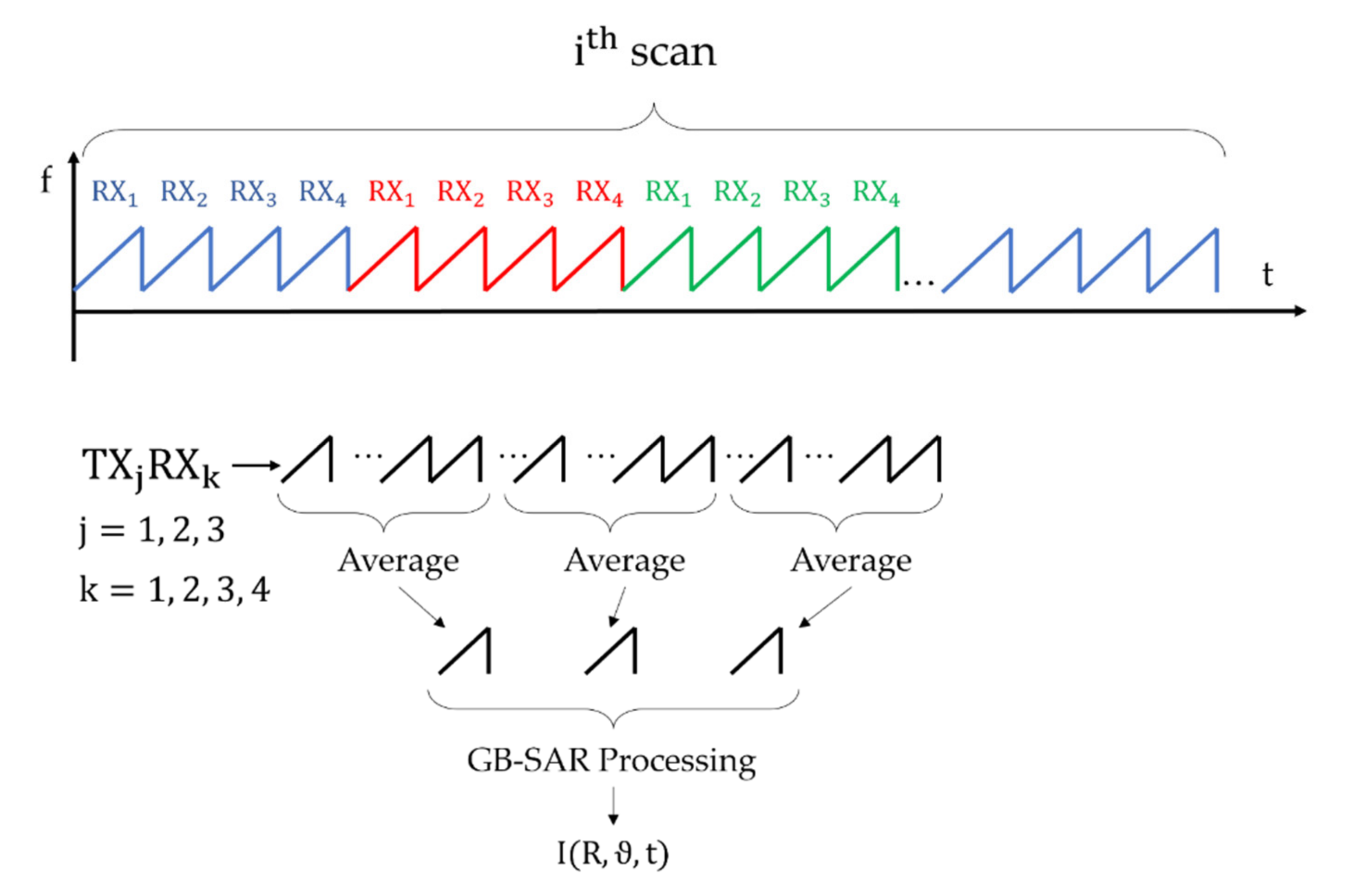
Figure 7 shows the data processing flow schematically. The signals of the same TX-RX couple were grouped and time averaged for reducing the computational time. Indeed, each single scan produces more than 50,000 chirps (12,500 chirps for each receiving antenna) and the computational cost could be very expensive in terms of time and memory space.
The reduced chirps were spaced with a step of about . The reduction factor depends on the radar parameters, and it is typically between 100 and 150.
After averaging, the Fast Fourier Transform (FFT) of each (averaged) chirp was calculated along the range. The result of FFT was focused on a plane image (typically horizontal or vertical) by considering the electromagnetic path from the antenna position to each point of the plane. This is basically a back propagation processing, as described in [26]. Kaiser windows () were applied along the range, azimuth, and elevation direction for lowering the side lobes. The result of focusing processing is a complex number, , which depends on range (R), azimuth or elevation angle (), and time (t).
The time-averaging does not affect the focusing algorithm; indeed, it is a high pass for the continuous signals.
The amplitude of represents the focused radar image. The phase can be used for radar interferometry:
with as the interferometric phase, ds as the displacement, and as the wavelength of the central frequency. The symbol represents the phase of a complex number.
3. Results
The radar was tested in a controlled scenario and during an in-field monitoring campaign on the historical Vespucci bridge in Florence, Italy.
3.1. Controlled Scenario
In order to evaluate the performance of the GB-SAR, the radar was operated in a controlled scenario. During these tests, the azimuth and elevation resolutions, and the interferometric uncertainty, were experimentally measured.
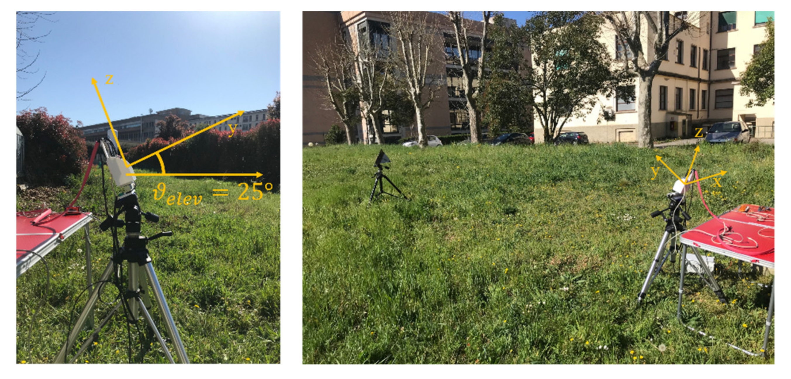
A corner reflector was located in front of the radar at a distance of . The radar and the target were at the same height above the ground. Then, the radar was back-tilted with an elevation angle of 25°, as shown in Figure 8. Using this method, the target appeared to be lower than the radar. A micrometric displacement stage was fixed to the corner reflector. The micrometric displacement stage allows us to move the target using a micrometric screw with high reliability. The radar parameters are reported in Table 1.
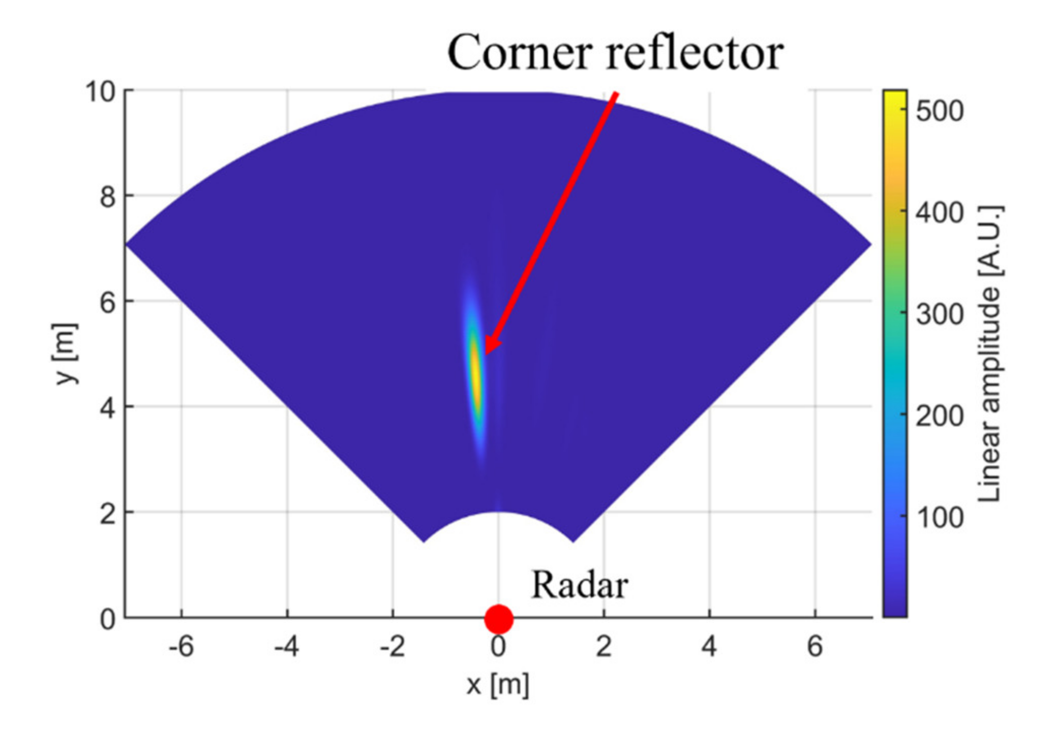
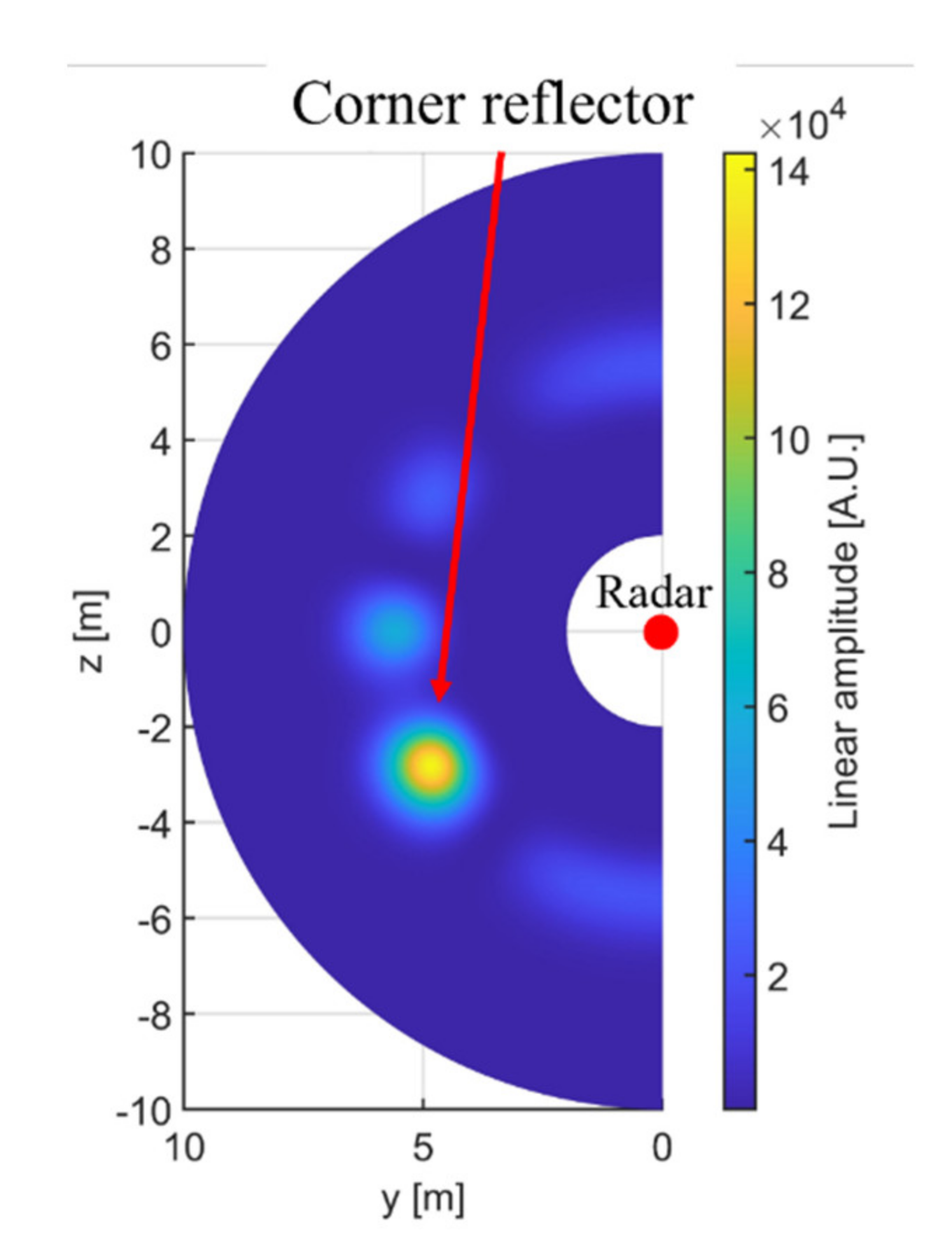
The radar image can be focused on the vertical or horizontal plane. We focused the radar image on a horizontal x-y plane (Figure 9) by fixing the altitude, and on a vertical z-y plane (Figure 10) by fixing the abscissa. The altitude and the abscissa correspond to the target position.
Figure 9 shows the radar image focused on the horizontal plane at . The target position in this plane was on the left with respect to the radar at .
Figure 10 shows the radar image focused on the vertical plane at , which is the position retrieved in Figure 9. As we expected, the target was at , which corresponds to an elevation of about 30°. These two images demonstrate the 3D capability of the system.
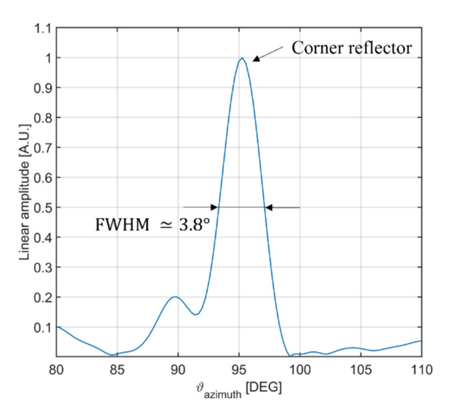
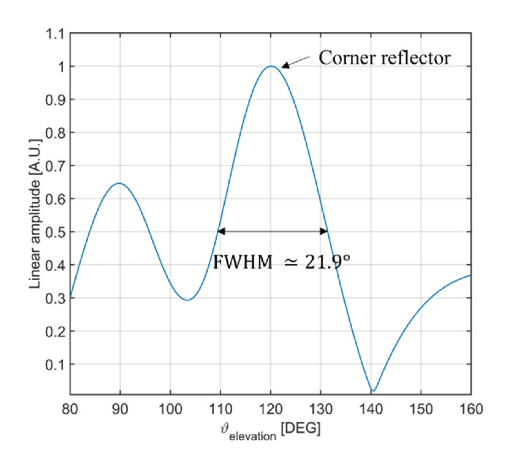
Figure 11 and Figure 12 show the normalized point spread functions (PSF) at the range of the target in terms of azimuth and elevation. We can estimate the angular resolution using the PSF. Indeed, the angular resolution can be retrieved using the full-width at half-maximum (FWHM) by:
where is the angular resolution. Equation (5) also considers the contribution of the Kaiser window to the resolution with the factor . This factor is equal to with .
The FWHM in azimuth was about 3.8° (Figure 11), and the FWHM in elevation was about 22° (Figure 12). Both values are in good agreement with theoretical values.
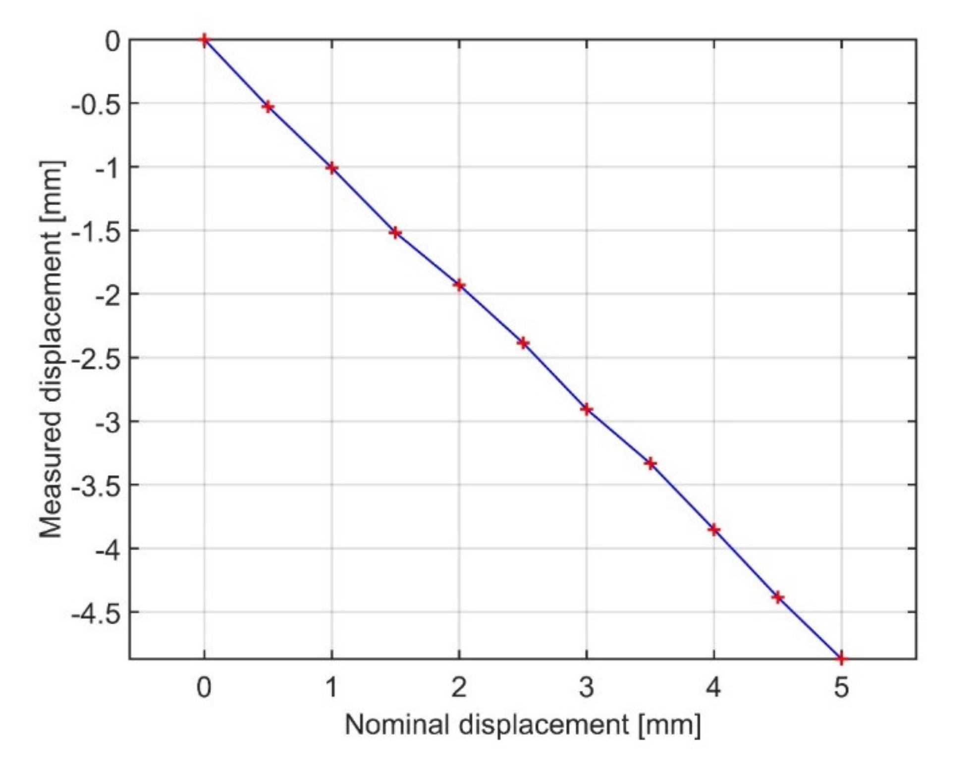
In order to verify the interferometric capability, the corner reflector was moved along the range direction with steps of 0.5 mm, towards the radar. The result of interferometric measurement is shown in Figure 13. The average displacement was and the standard deviation 0.04 mm. These values are in good agreement with the current GB-SAR [27,28] (the measurement uncertainty of conventional GB-SAR is about 0.1 mm).
3.2. Vespucci Bridge, Florence, Italy
Static and a dynamic monitoring were performed on the Vespucci bridge in Florence, Italy. The bridge was designed and built between 1955 and 1957. The bridge is composed of three spans and two pillars. Since 2018, the bridge has been the object of a renovation and monitoring plan for consolidating the two pillars and the stalls inside the carriage [8].
The monitoring campaign, presented in this work, was interested in the central span, which is about 53 m long and 6.5 m in height. Figure 14 shows the radar setup and the bridge span. The radar was located under the bridge, close to the right pillar of the central span in the middle of the carriage. The radar was back-tilted along the x-axis of about α = 19°. This value was considered during the focusing process. Figure 14a shows the reference system. The origin of the axis was in the middle of the radar scan. The x-y plan was leveled, so it can be considered on a horizonal plane. The z-axis was assumed to be vertical.
The radar was at below the bridge and the left pillar was at about from the radar. The radar was exactly in the center of the roadway.
Radar parameters are reported in Table 2.
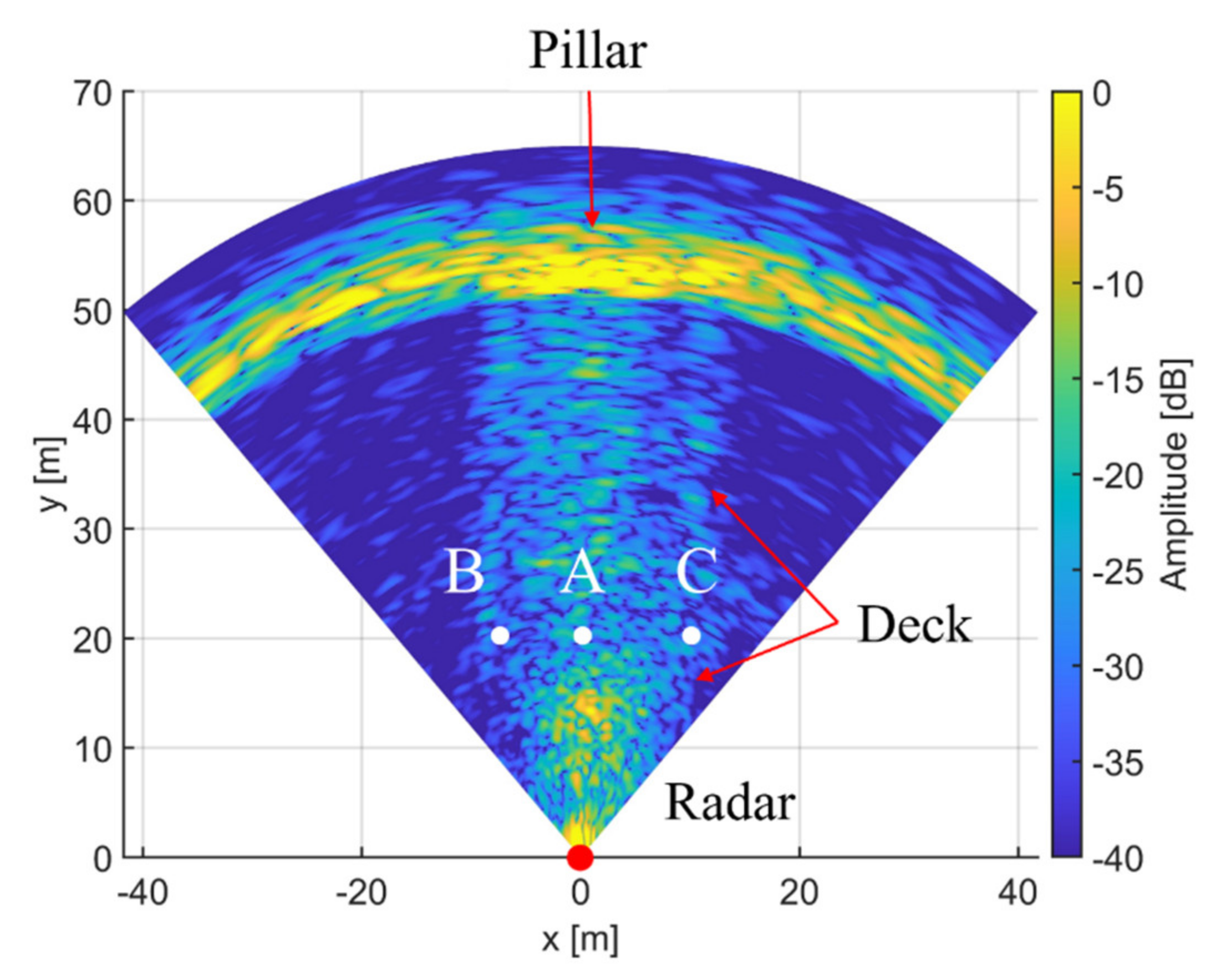
The focused image is shown in Figure 15. The echo was focused on a horizontal plane that corresponds to the bridge deck (z = 6.5 m). The deck shape is well recognizable, and the signal from the pillar generated high side lobes.
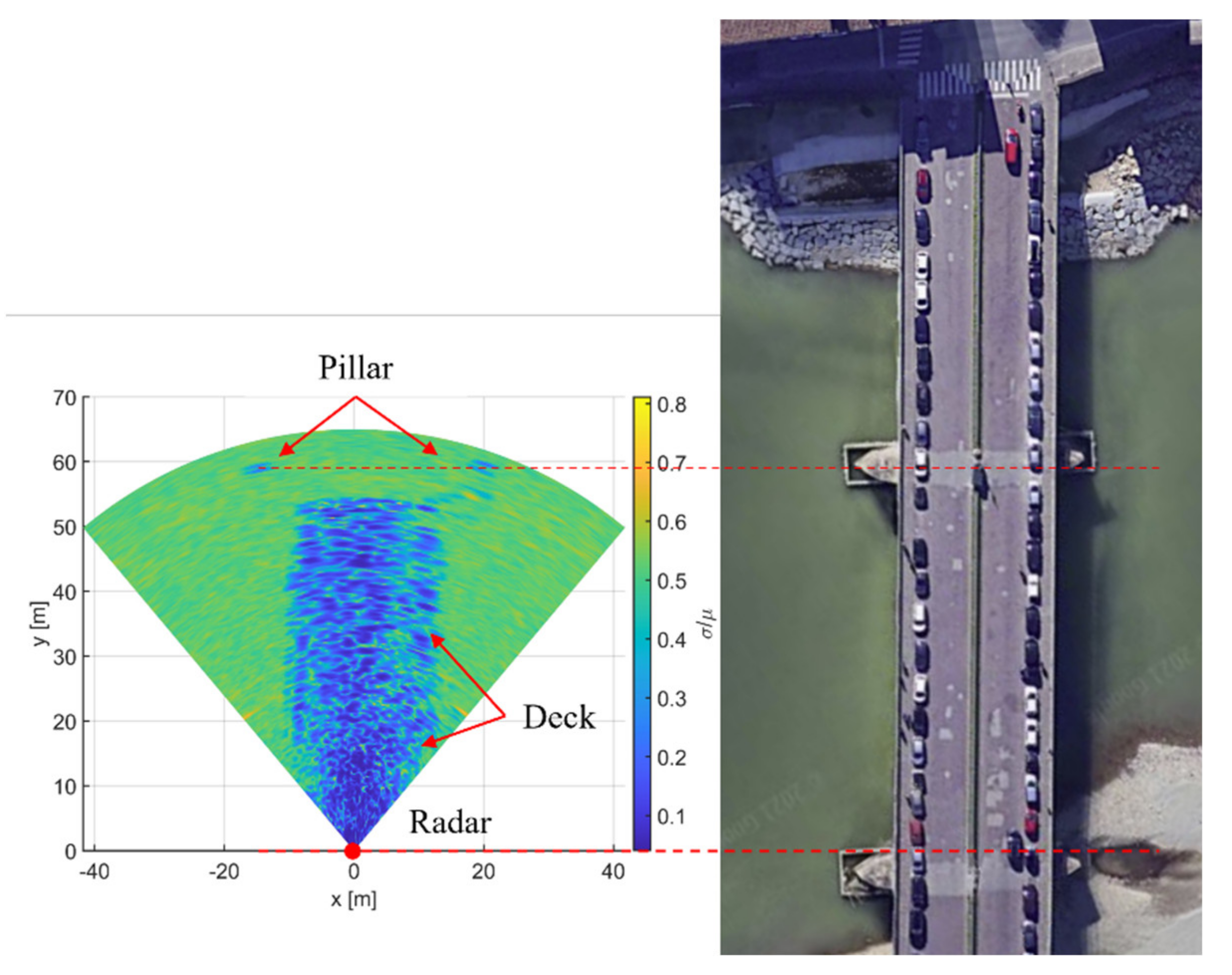
The index of dispersion [29] image was calculated for discriminating the coherent pixels in the radar image (see Figure 16). Generally speaking, the dispersion index of a permanent scatterer has to be lower than 0.3. This value corresponds to the blue color in Figure 16. Most of the targets on the deck can be considered as permanent scatterers.
We can clearly recognize the shape of the deck. It is also possible to see the left pillar wings that are covered by the pillar sidelobes in Figure 15.
The static test was performed using a truck of 25 tons. The truck approached the bridge from the left side, and it was stationed in the center of the deck, on the left carriage, for almost 23 min.
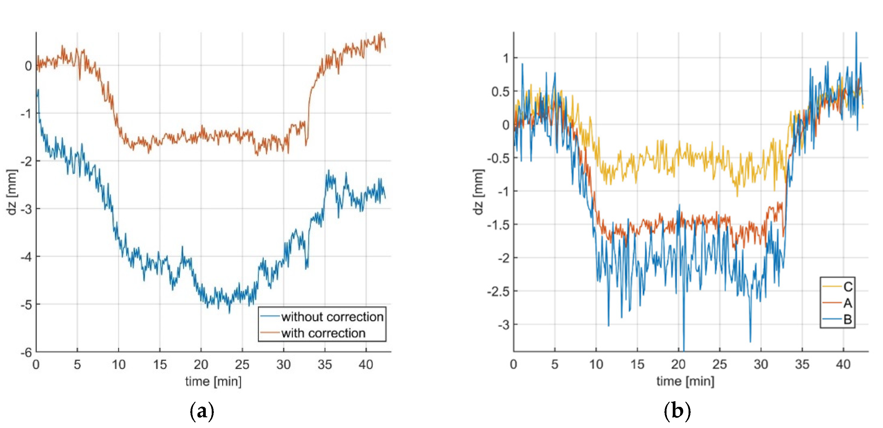
Figure 17a shows the vertical displacement in time of point A with and without any atmospheric correction. Point A was in . It is evident that the atmospheric changes generate false movements that have to be compensated. So, we applied an atmospheric correction as, for example, reported in [30,31]. The target at , , and was used as a stable reference target for the atmospheric correction. This target corresponds to the left pillar, which can be surely considered stable throughout the duration of the test.
The comparison between the displacement of point A, B, and C (see Figure 15), after atmospheric correction, is shown in Figure 17b. Point B was in , and point C was in .
The track was located on the left carriage, as visible by the asymmetry between left (target B) and right (target C). Indeed, the maximum displacement of target C was about , while for target B it was about .
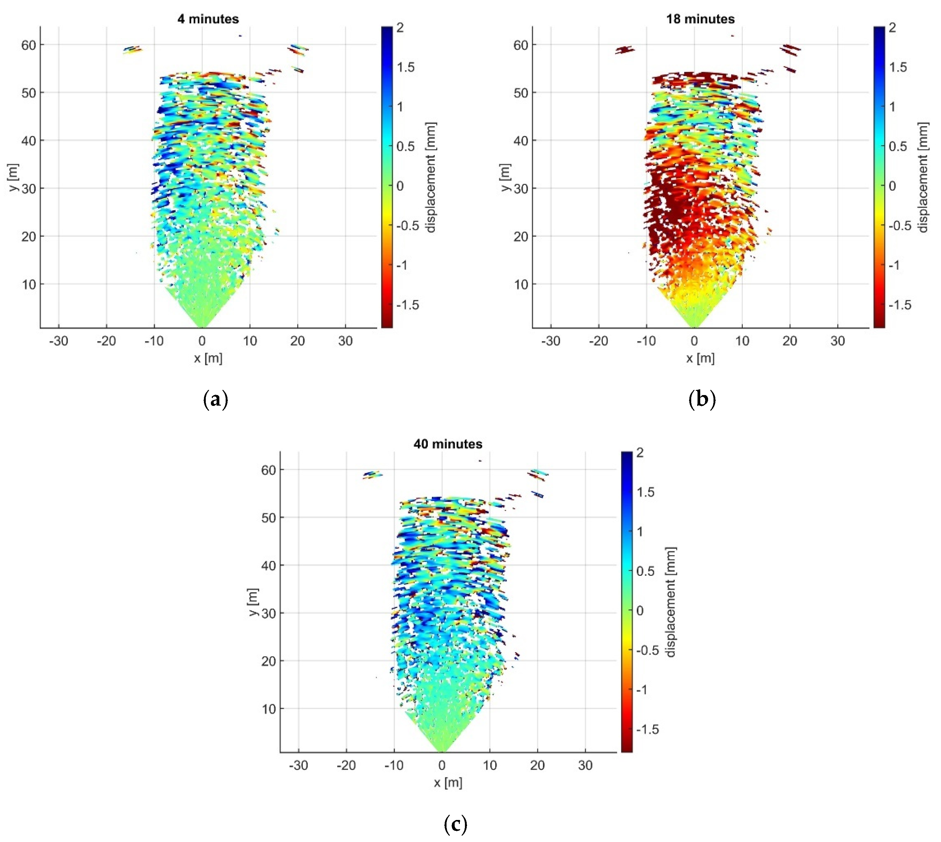
Finally, in Figure 18 some displacement maps are reported. The map shows the displacement map after 4 min (Figure 18a), 18 min (Figure 18b), and 40 min (Figure 18c).
The displacement maps confirm the displacement asymmetry of Figure 17b. Indeed, the maximum displacement was in the area between and on the left carriage (negative x).
The blue areas (displacement along positive z direction) in Figure 18a,c can be associated with the structure of the bridge as discussed in [10].
For evaluating the capability of the radar to perform dynamic structural tests, the radar was rotated 90° along the y axis (see Figure 14a), as shown in Figure 19. The radar parameters were the same as those used for the static test. The sampling rate of each transmitting antenna was 529.10 Hz and reduced to 105.82 Hz by averaging, as described in Figure 7.
For the dynamic test, the truck crossed the bridge in both directions at an average speed between 23 km/h and 50 km/h. The truck’s speed was limited by the bridge status.
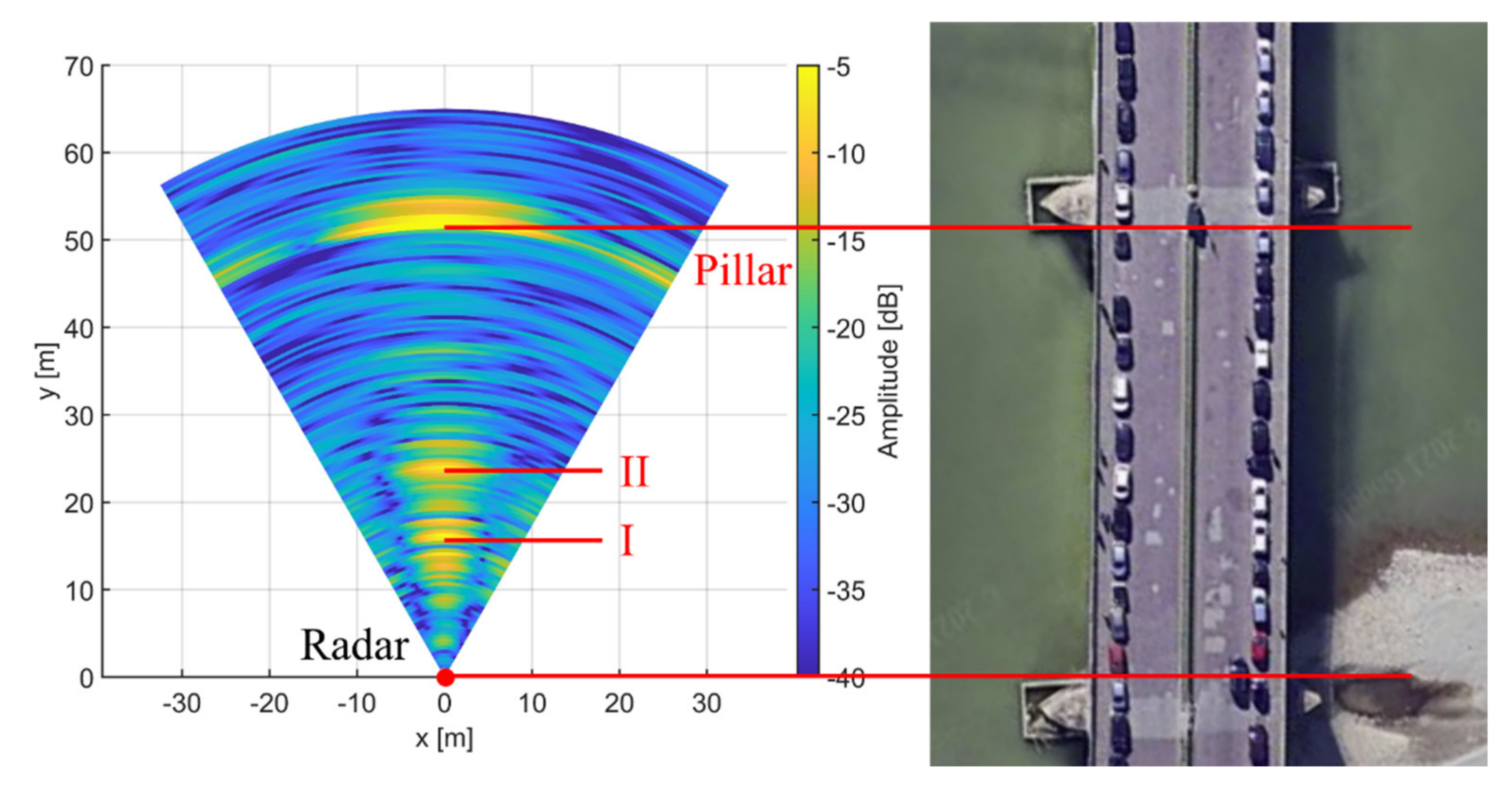
The focused radar image is shown in Figure 20 As the radar head does not move during the acquisition, only the virtual antennas of MIMO are considered in the focusing algorithm. Obviously, the angular resolution is not as high as when the radar head can move along its mechanical guide.
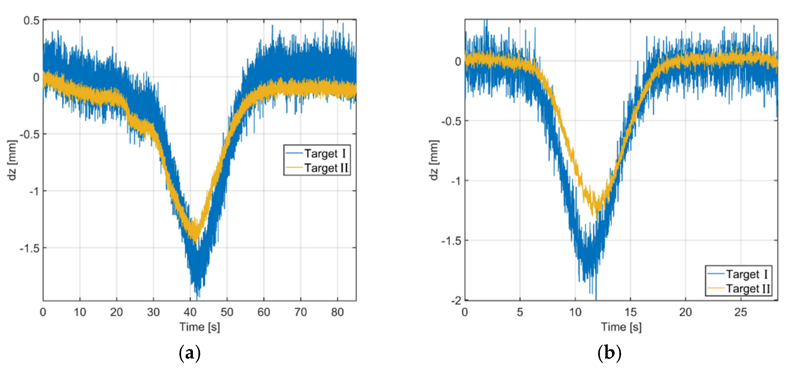
The measured displacement in time of target I and target II (labeled in Figure 20) is shown in Figure 21. Target I was at 16 m in front of the radar, and target II was at 24 m. The pillar was at about 53 m. In Figure 21a, the truck approached the bridge from the left side, and in Figure 21b the truck approached the bridge from the right side. Note that the displacement of point B is affected by a larger error. This is just due to the lower signal amplitude of point II, which is at a larger distance from the radar.
4. Discussion
The proposed 77 GHz GB-SAR with 3D capability was tested in a controlled environment to demonstrate the 3D capability and to determine the experimental performances. The azimuth and elevation resolution were retrieved (, ), and they were in good agreement with the theoretical value. Additionally, the displacement capability was evaluated, and the displacement accuracy was about 0.04 mm.
The radar was also used in a real scenario for monitoring the Vespucci bridge, Florence, Italy. The sensor was able to detect left/right movement of the bridge during static monitoring. Indeed, the truck was located on the left roadway. The results of this monitoring are reported in Figure 17 and Figure 18. It is possible to note a difference between left and right displacement in Figure 17b and Figure 18b.
The radar was also used for dynamic monitoring by measuring the displacement due to truck movement. In this case, no further analysis was carried out due to the speed limits.
5. Conclusions
In this paper, a fast interferometric MIMO GB-SAR operating at 77 GHz is proposed. The MIMO GB-SAR is based on a single-chip radar. The radar can acquire 3D images in less than 8 s with a theoretical azimuth resolution of 1.75° and an elevation resolution of 10°.
The system is also able to perform dynamic structural tests with an angular resolution of 10° and acquisition frequency up to 500 Hz.
The performance of the radar, in terms of angular resolution and interferometric capability, was preliminarily tested in a controlled environment.
Furthermore, the sensor was operated during a monitoring campaign on the historical Vespucci bridge in Florence, Italy. The MIMO GB-SAR was able to provide the displacement map on the deck surface with 0.125 Hz sampling frequency. Finally, operating in the only-MIMO modality, the radar was able to acquire the dynamic displacements of the deck stimulated by a truck crossing the bridge at speeds between 23 km/h and 50 km/h.
In conclusion, the fast MIMO GB-SAR proposed in this paper is able to perform both 3D GB-SAR acquisition in less than 8 s and dynamic measurement (at 500 Hz sampling frequency), even if with poor azimuth resolution. The proposed sensor is far from ready for industrialization, but it opens many practical applications precluded by slower and bulkier radar systems.
Author Contributions
Conceptualization, M.P. and L.M.; methodology, T.C. and L.M.; software, T.C.; validation, L.M. and A.B.; formal analysis, L.M.; resources, M.P.; data curation, A.B.; writing—original draft preparation, L.M.; writing—review and editing, L.M., M.P. and A.B.; supervision, M.P. and L.M.; project administration, M.P.; funding acquisition, M.P. All authors have read and agreed to the published version of the manuscript.
Funding
This work was supported in part by the Fondazione Cassa di Risparmio di Firenze Grant: 2323.1639”.
Conflicts of Interest
The authors declare no conflict of interest.
References
- Pieraccini, M.; Miccinesi, L. Ground-Based Radar Interferometry: A Bibliographic Review. Remote Sens. 2019, 11, 1029. [Google Scholar] [CrossRef] [Green Version]
- Pieraccini, M. Monitoring of civil infrastructures by interferometric radar: A review. Sci. World J. 2013, 2013, 786961. [Google Scholar] [CrossRef] [PubMed]
- Luzi, G.; Crosetto, M.; Fernández, E. Radar interferometry for monitoring the vibration characteristics of buildings and civil structures: Recent case studies in Spain. Sensors 2017, 17, 669. [Google Scholar] [CrossRef] [PubMed] [Green Version]
- Shao, Z.; Zhang, X.; Li, Y.; Jiang, J. A comparative study on radar interferometry for vibrations monitoring on different types of bridges. IEEE Access 2018, 6, 29677–29684. [Google Scholar] [CrossRef]
- Dei, D.; Mecatti, D.; Pieraccini, M. Static testing of a bridge using an interferometric radar: The case study of ‘ponte degli alpini,’ Belluno, Italy. Sci. World J. 2013, 2013, 7. [Google Scholar] [CrossRef] [PubMed]
- Wang, Z.; Li, Z.; Mills, J. A new approach to selecting coherent pixels for ground-based SAR deformation monitoring. ISPRS J. Photogramm. Remote. Sens. 2018, 144, 412–422. [Google Scholar] [CrossRef] [Green Version]
- Pieraccini, M.; Miccinesi, L. An Interferometric MIMO Radar for Bridge Monitoring. IEEE Geosci. Remote. Sens. Lett. 2019, 16, 1383–1387. [Google Scholar] [CrossRef]
- Pieraccini, M.; Miccinesi, L.; Rojhani, N. Monitoring of Vespucci bridge in Florence, Italy using a fast real aperture radar and a MIMO radar. In Proceedings of the IEEE International Geoscience and Remote Sensing Symposium, Yokohama, Japan, 28 July–2 August 2019; pp. 1982–1985. [Google Scholar] [CrossRef]
- Tarchi, D.; Oliveri, F.; Sammartino, P.F. MIMO Radar and Ground-Based SAR Imaging Systems: Equivalent Approaches for Remote Sensing. IEEE Trans. Geosci. Remote. Sens. 2013, 51, 425–435. [Google Scholar] [CrossRef]
- Hu, C.; Wang, J.; Tian, W.; Zeng, T.; Wang, R. Design and Imaging of Ground-Based Multiple-Input Multiple-Output Synthetic Aperture Radar (MIMO SAR) with Non-Collinear Arrays. Sensors 2017, 17, 598. [Google Scholar] [CrossRef] [PubMed]
- Cong, X.; Liu, J.; Long, K.; Liu, Y.; Zhu, R.; Wan, Q. Millimeter-wave spotlight circular synthetic aperture radar (scsar) imaging for Foreign Object Debris on airport runway. In Proceedings of the 12th International Conference on Signal Processing (ICSP), Hangzhou, China, 19–23 October 2014; pp. 1968–1972. [Google Scholar]
- Steiner, M.; Grebner, T.; Waldschmidt, C. Millimeter-Wave SAR-Imaging With Radar Networks Based on Radar Self-Localization. IEEE Trans. Microw. Theory Tech. 2020, 68, 4652–4661. [Google Scholar] [CrossRef]
- Hasch, J.; Topak, E.; Schnabel, R.; Zwick, T.; Weigel, R.; Waldschmidt, C. Millimeter-Wave Technology for Automotive Radar Sensors in the 77 GHz Frequency Band. IEEE Trans. Microw. Theory Tech. 2012, 60, 845–860. [Google Scholar] [CrossRef]
- Feger, R.; Haderer, A.; Stelzer, A. Experimental verification of a 77-GHz synthetic aperture radar system for automotive applications. In Proceedings of the 2017 IEEE MTT-S International Conference on Microwaves for Intelligent Mobility (ICMIM); Institute of Electrical and Electronics Engineers (IEEE), Nagoya, Japan, 19–21 March 2017; pp. 111–114. [Google Scholar]
- Daria, D.; Amoroso, G.; Bicci, A.; Coppi, F.; Cecchetti, M.; Rossi, M.; Falcone, P. Advanced tomographic tool for HYDRA radar system. In Proceedings of the 12th European Conference on Synthetic Aperture Radar, Aachen, Germany, 4–7 June 2018; pp. 1–3. [Google Scholar]
- Cecchetti, M.; Rossi, M.; Coppi, F. Performance evaluation of a new MMW Arc SAR system for underground deformation monitoring. In Active and Passive Microwave Remote Sensing for Environmental Monitoring II; SPIE: Bellingham, WA, USA, 2018; Volume 10788, p. 1078801. [Google Scholar]
- Gale, S.; Farrington, L.; Bergstrom, P.; Suikkanen, M.; Boldrini, N.; Rubino, M.; Coli, N.; Naude, S.; Stopka, C.; Preston, C. Monitoring applications for safe mining practices: Case studies of sub-bench scale failures in hard rock and coal open cut mines. In Proceedings of the 2020 International Symposium on Slope Stability in Open Pit Mining and Civil Engineering, Perth, Australia, 12–14 May 2020; 2020; pp. 1563–1576. [Google Scholar]
- Giannino, F.; Manacorda, G.; Simi, A.; Cecchetti, M.; Vacca, D. Radar for structural monitoring and assets mapping. In Proceedings of the 2020 IEEE Radar Conference (RadarConf20), Institute of Electrical and Electronics Engineers (IEEE), Firenze, Italia, 21–25 September 2020; 2020; pp. 1–3. [Google Scholar]
- Romeo, S.; Cosentino, A.; Giani, F.; Mastrantoni, G.; Mazzanti, P. Combining Ground Based Remote Sensing Tools for Rockfalls Assessment and Monitoring: The Poggio Baldi Landslide Natural Laboratory. Sensors 2021, 21, 2632. [Google Scholar] [CrossRef] [PubMed]
- Miccinesi, L.; Michelini, A.; Pieraccini, M. Blurring/Clutter Mitigation in Quarry Monitoring by Ground-Based Synthetic Aperture Radar. IEEE Trans. Geosci. Remote. Sens. 2021, 1–8, Early Access. [Google Scholar] [CrossRef]
- Texas Instruments. AWR1843BOOST and IWR1843BOOST Single-Chip mmWave Sensing Solution User’s Guide (Rev. B). Available online: https://www.ti.com/tool/AWR1843BOOST (accessed on 1 September 2021).
- Texas Instruments. Mmwave-Studio. Available online: https://www.ti.com/tool/MMWAVE-STUDIO (accessed on 1 September 2021).
- Texas Instruments. Programming Chirp Parametersin TI Radar Devices. Available online: https://www.ti.com/lit/an/swra553a/swra553a.pdf?ts=1631521293806&ref_url=https%253A%252F%252Fwww.ti.com%252Fsitesearch%252Fdocs%252Funiversalsearch.tsp%253FlangPref%253Den-US%2526searchTerm%253DProgramming%2BChirp%2BParameters%2Bin%2BTI%2BRadar%2BDevices%2526nr%253D540 (accessed on 1 September 2021).
- Ciattaglia, G.; de Santis, A.; Disha, D.; Spinsante, S.; Castellini, P.; Gambi, E. Performance Evaluation of Vibrational Measurements through mmWave Automotive Radars. Remote. Sens. 2021, 13, 98. [Google Scholar] [CrossRef]
- Pieraccini, M.; Miccinesi, L.; Morini, F. An Interferometric W-BAND Radar for Large Structures Monitoring. In Proceedings of the IEEE International Geoscience and Remote Sensing Symposium, Waikoloa, HI, USA, 26 September–2 October 2020; pp. 4207–4210. [Google Scholar] [CrossRef]
- Pieraccini, M.; Miccinesi, L. ArcSAR: Theory, Simulations, and Experimental Verification. IEEE Trans. Microw. Theory Tech. 2016, 65, 293–301. [Google Scholar] [CrossRef]
- Pieraccini, M.; Fratini, M.; Parrini, F.; Atzeni, C.; Bartoli, G. Interferometric radar vs. accelerometer for dynamic monitoring of large structures: An experimental comparison. NDT E Int. 2008, 41, 258–264. [Google Scholar] [CrossRef]
- Castagnetti, C.; Bassoli, E.; Vincenzi, L.; Mancini, F. Dynamic assessment of masonry towers based on terrestrial radar interferometer and accelerometers. Sensors 2019, 19, 1319. [Google Scholar] [CrossRef] [PubMed] [Green Version]
- Ferretti, A.; Prati, C.; Rocca, F. Permanent scatterers in SAR interferometry. IEEE Trans. Geosci. Remote. Sens. 2001, 39, 8–20. [Google Scholar] [CrossRef]
- Yang, H.; Liu, J.; Peng, J.; Wang, J.; Zhao, B.; Zhang, B. A method for GB-InSAR temporal analysis considering the atmospheric correlation in time series. Nat. Hazards 2020, 104, 1465–1480. [Google Scholar] [CrossRef]
- Karunathilake, A.; Sato, M. Atmospheric Phase Compensation in Extreme Weather Conditions for Ground-Based SAR. IEEE J. Sel. Top. Appl. Earth Obs. Remote. Sens. 2020, 13, 3806–3815. [Google Scholar] [CrossRef]
Figure 1.
Scheme of proposed GB-SAR.

Figure 2.
Flow chart of acquisition system of W-band GB-SAR.

Figure 3.
Working principle of 77 GHz radar.

Figure 4.
Chirp geometry of AWR1843.

Figure 5.
Prototype of GB-SAR (a), and details of the antennas’ configuration (b).

Figure 6.
Prototype of interferometric radar.

Figure 7.
Data analysis procedure.

Figure 8.
GB-SAR setup during the measurement in the controlled scenario.

Figure 9.
Radar image focused on the horizontal plane at .

Figure 10.
Radar image focused on the vertical plane at .

Figure 11.
Point spread function in terms of azimuth.

Figure 12.
Point spread function in terms of elevation.

Figure 13.
Displacement measured by GB-SAR in controlled scenario.

Figure 14.
Radar setup (a) during the measurement campaign at Vespucci bridge (b).

Figure 15.
Radar image of Vespucci bridge focused on the horizontal plane at . The targets A, B, C were used for the displacement analysis.
Figure 15.
Radar image of Vespucci bridge focused on the horizontal plane at . The targets A, B, C were used for the displacement analysis.

Figure 16.
Index of dispersion of radar images of Vespucci bridge focused on the horizontal plane at .
Figure 16.
Index of dispersion of radar images of Vespucci bridge focused on the horizontal plane at .

Figure 17.
Vertical component of displacement during time: (a) comparison between vertical displacement with and without atmospheric correction; (b) comparison between three points at the same distance located on the right, on the center, and on the left of the carriage.
Figure 17.
Vertical component of displacement during time: (a) comparison between vertical displacement with and without atmospheric correction; (b) comparison between three points at the same distance located on the right, on the center, and on the left of the carriage.

Figure 18.
Map of vertical displacement of the bridge deck: (a) after 4 min; (b) after 18 min; and (c) after 40 min.
Figure 18.
Map of vertical displacement of the bridge deck: (a) after 4 min; (b) after 18 min; and (c) after 40 min.

Figure 19.
Radar setup for dynamic test.

Figure 20.
Radar image of Vespucci bridge focused using the MIMO system.

Figure 21.
Measured displacement of target I and II (see Figure 20): (a) the truck approaches the bridge from the left side; (b) the truck approaches the bridge from the right side.
Figure 21.
Measured displacement of target I and II (see Figure 20): (a) the truck approaches the bridge from the left side; (b) the truck approaches the bridge from the right side.

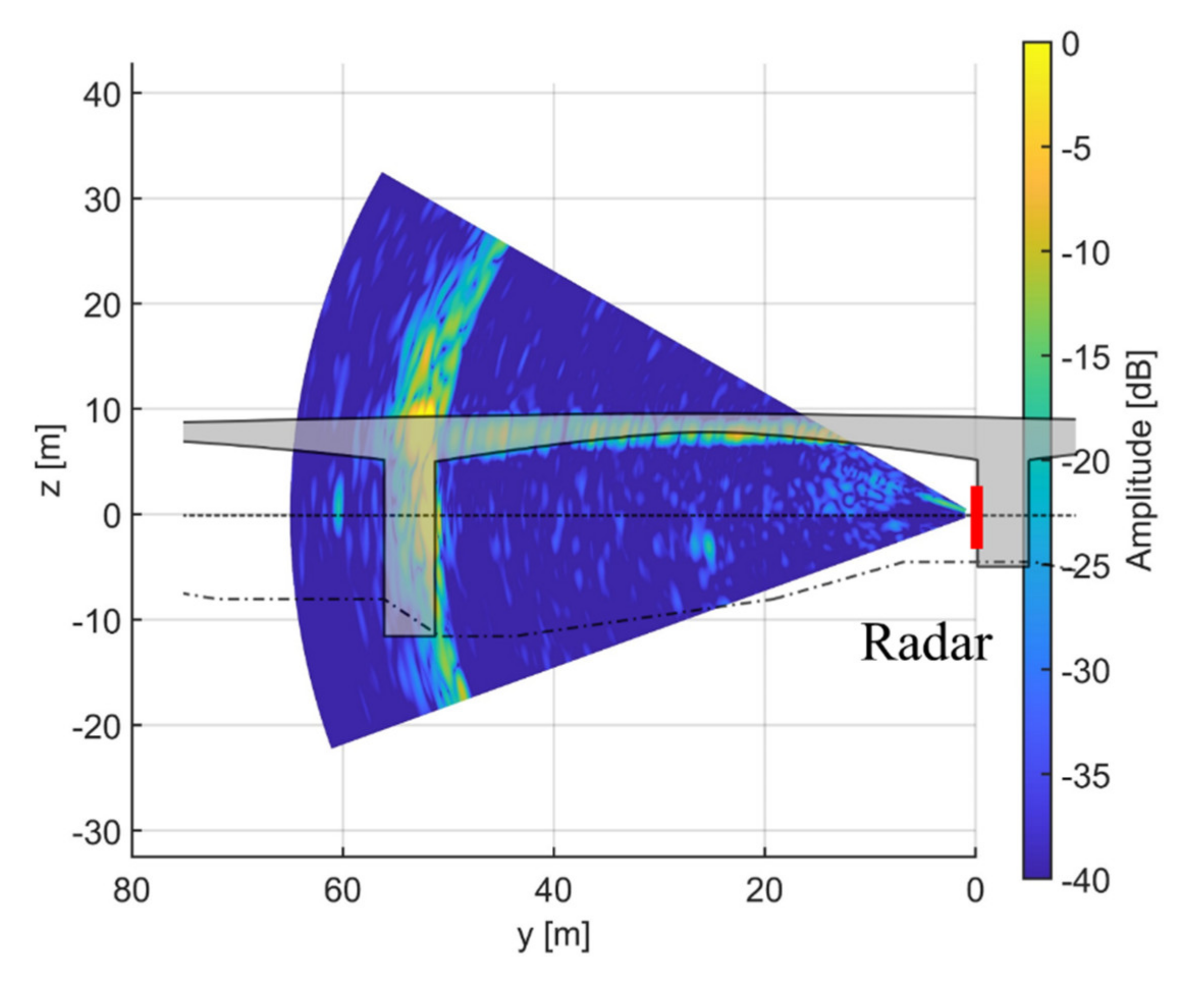
Figure 22.
Radar image with vertical GB-SAR focused on the plane .


Table 1.
Radar parameters in controlled scenario.
| Parameter | Description | |
|---|---|---|
| Numbers of ADC samples | 256 | |
| Slope | 4.007 MHz/μs | |
| Starting frequency | 77 GHz | |
| Bandwidth | 103 MHz | |
| Chirp periodicity | 6.3 μs | |
| Scan time | ~8 s | |
| Actuator speed | 8 mm/s |
Table 2.
Radar parameters during the Vespucci bridge monitoring.
| Parameter | Description | |
|---|---|---|
| Numbers of ADC samples | 1024 | |
| Slope | 4.007 MHz/μs | |
| Starting frequency | 77 GHz | |
| Bandwidth | 103 MHz | |
| Chirp periodicity | 6.3 μs | |
| Scan time | ~8 s | |
| Actuator speed | 8 mm/s |
Publisher’s Note: MDPI stays neutral with regard to jurisdictional claims in published maps and institutional affiliations. |
© 2021 by the authors. Licensee MDPI, Basel, Switzerland. This article is an open access article distributed under the terms and conditions of the Creative Commons Attribution (CC BY) license (https://creativecommons.org/licenses/by/4.0/).
Share and Cite
MDPI and ACS Style
Miccinesi, L.; Consumi, T.; Beni, A.; Pieraccini, M. W-band MIMO GB-SAR for Bridge Testing/Monitoring. Electronics 2021, 10, 2261. https://doi.org/10.3390/electronics10182261
AMA Style
Miccinesi L, Consumi T, Beni A, Pieraccini M. W-band MIMO GB-SAR for Bridge Testing/Monitoring. Electronics. 2021; 10(18):2261. https://doi.org/10.3390/electronics10182261
Chicago/Turabian StyleMiccinesi, Lapo, Tommaso Consumi, Alessandra Beni, and Massimiliano Pieraccini. 2021. "W-band MIMO GB-SAR for Bridge Testing/Monitoring" Electronics 10, no. 18: 2261. https://doi.org/10.3390/electronics10182261
Note that from the first issue of 2016, this journal uses article numbers instead of page numbers. See further details here.