Design of Composite Disturbance Observer and Continuous Terminal Sliding Mode Control for Piezoelectric Nanopositioning Stage

Abstract

The nonlinearities of piezoelectric actuators and external disturbances of the piezoelectric nanopositioning stage impose great, undesirable influences on the positioning accuracy of nanopositioning stage systems. This paper considers nonlinearities and external disturbances as a lumped disturbance and designs a composite control strategy for the piezoelectric nanopositioning stage to realize ultra-high precision motion control. The proposed strategy contains a composite disturbance observer and a continuous terminal sliding mode controller. The composite disturbance observer can estimate both periodic and aperiodic disturbances so that the composite control strategy can deal with the disturbances with high accuracy. Meanwhile, the continuous terminal sliding mode control is employed to eliminate the chattering phenomenon and speed up the convergence rate. The simulation and experiment results show that the composite control strategy achieves accurate estimation of different forms of disturbances and excellent tracking performance.

1. Introduction

In the field of manufacturing and processing of micro and nano equipment, the piezoelectric nanopositioning stage is widely used, due to its advantages of large driving force and fast response speed. On the basis of this nanopositioning stage, many kinds of high-precision engineering studies can be carried out, such as scanning probe microscope [1] and cell injection [2]. It is well known that the proportional–integral (PI) control scheme is already widely applied in the piezoelectric nanopositioning stage, due to its relative simple implementation [3,4].

However, the piezoelectric nanopositioning stage is driven by piezoelectric actuators that exhibit hysteresis nonlinearity, creep nonlinearity and badly damped vibration nonlinearity [5,6]. In actual working conditions, the nanopositioning stage is affected by a variety of disturbances [7]. It is difficult to achieve high precision motion control requirements of the nanopositioning stage using conventional linear control methods. For this reason, nonlinear control strategies have been applied to the nanopositioning stage, e.g., sliding mode control [8,9] and robust control [10]. As one of them, sliding mode control (SMC) has become a common control method in the nanopositioning stage systems for its strong robustness and capacity of disturbance rejection. In order to further improve the performance of sliding mode control, some scholars designed terminal sliding mode control (TSMC) based on the construction of nonlinear sliding surface to achieve convergence in finite time and reduce the steady-state tracking error [8,11,12].

Neither conventional SMC nor TSMC can avoid the phenomenon of chattering due to the existence of the high frequency switching effect [13]. In the nanopositioning stage system, chattering may seriously affect control performance, cause system instability and even damage the piezoelectric actuators [14]. So, the elimination of the chattering phenomenon has attracted more and more attention recently. For example, adaptive sliding mode control [14,15], fuzzy sliding mode control [16], discrete-time sliding mode control [8,17], neural dynamic sliding mode control [18] and integral sliding mode control [19] have been proposed to mitigate the adverse effects of the chattering phenomenon. It has been reported that designing a continuous sliding mode control law to replace the discontinuous law, e.g., continuous TSMC (CTSMC) can reduce the impact of the chattering [20,21]. The CTSMC method is able to not only eliminate chattering, but also realize the convergence of the system state in finite time. However, as mentioned before, the positioning accuracy of the piezoelectric nanopositioning stage is severely affected by nonlinear characteristics and external disturbance, so high gain is required to achieve the desired control performance for CTSMC method, which may make the control energy beyond the limitation of the real actuator.

In terms of disturbance rejection, the nonlinear characteristics and external disturbances are lumped together and then estimated for feedforward compensation; many common approaches have been proposed to estimate disturbances, including the unknown input observer (UIO) [22], the disturbance observer (DOB) [23,24], and the extended state observer (ESO) [25,26]. ESO is considered to be an effective method, which regards the lumped disturbance as a new system state; then, the state and disturbance of the system can be observed by simple calculation. Then, the observed disturbance is compensated in the feedforward channel to improve the performance of the system [27,28]. Although ESO-based control methods are widely used in industry, satisfactory results are difficult to achieve in estimating periodic disturbances [29,30,31]. However, there are friction transmission and mechanical resonance in the work of the piezoelectric nanopositioning stage, to which it is easy to bring periodic disturbance. For better control performance, a composite observer is needed to estimate both periodic and aperiodic disturbances simultaneously.

In this paper, a composite control strategy which combines composite disturbance observer and continuous terminal sliding mode control to realize the high-precision control of the piezoelectric nanopositioning stage is proposed. The CTSMC is used to improve the dynamic performance of the piezoelectric nanopositioning stage system and realize finite time convergence, while composite disturbance is proposed to precisely estimate the lumped disturbance and carry out the feedforward compensation. The proposed strategy has the following advantages: (1) finite time convergence, (2) continuous rather than discontinuous control action, and (3) accurate estimation of both periodic and aperiodic disturbances. The simulation and experimental results show that the proposed control strategy can significantly improve the tracking performance of the system.

The remaining parts of the paper are organized as follows. The model of the piezoelectric nanopositioning stage and conventional control design are introduced in Section 2. Section 3 shows the design of the new control strategy. Then, Section 4 gives the simulations and experimental results. The research conclusions are summarized in Section 5.

2. Modeling and Conventional Control Design

2.1. Modeling of the Piezoelectric Nanopositioning Stage

Applying pressure on the surface of piezoelectric material can produce electric charge. This direct piezoelectric effect, also known as the generator or sensor effect, converts mechanical energy into electrical energy. On the contrary, when a certain voltage is applied, the inverse piezoelectric effect can change the length of such materials. This actuator effect converts electrical energy into mechanical energy. The piezoelectric nanopositioning stage is a kind of driving equipment that uses the inverse piezoelectric effect of piezoelectric ceramics, friction transmission and the principle of elastic resonance deformation amplification to promote the movement.

The dynamics model of the piezoelectric nanopositioning stage can be described as follows [14]:

$$m\ddot{x}+p\dot{x}+qx+h=ku,$$

(1)

where u is the input voltage, x is the output displacement, h is the lumped disturbance that consists of the nonlinearities and external disturbances, k denotes the piezoelectric coefficient, while m, p and q represent the mass, damping coefficient, and stiffness of the piezoelectric nanopositioning stage, respectively.

The position x is defined as $x_1=x$ and its derivative is defined as $x_2={\dot{x}}_1$. The dynamics model of the stage can be rewritten as follows:

$$\left\{\begin{array}{c}{\dot{x}}_1=x_2,\hfill \\ {\dot{x}}_2=a_1{x}_1+a_2{x}_2+b_{0}u+d,\hfill \\ y=x_1,\hfill \end{array}\right.$$

(2)

where:

$$a_1=-\frac{q}{m},a_2=-\frac{p}{m},b_0=\frac{k}{m},d=-\frac{h}{m},$$

(3)

and d is the lumped disturbance in system (2).

2.2. Analysis of Disturbances in the Piezoelectric Nanopositioning Stage

The purpose of this section is to analyze the specific composition and source of lumped disturbance d in system (2).

(1) The nonlinearities: As mentioned before, hysteresis nonlinearity, creep nonlinearity and badly damped vibration nonlinearity are the inherent nonlinearities of the piezoelectric nanopositioning stage. Hysteresis nonlinearity is the factor to reduce the displacement output accuracy of the piezoelectric nanopositioning stage, which is manifested in the non-coincidence of voltage and displacement curves. Creep nonlinearity means that when the voltage applied to the stage does not change, the displacement value is not stable at a fixed value, but changes over time and reaches a stable value after a certain time, which affects the stability of the control system. Badly damped vibration nonlinearity of the piezoelectric nanopositioning stage may cause the problem of low gain margin, which limits the improvement of the response speed of the stage and the control bandwidth of the system.

(2) External disturbances: While the piezoelectric nanopositioning stage works, it is affected by many kinds of external disturbances. When the external input signal contains high-frequency components, it is easy to excite the mechanical resonance of the system, resulting in the jitter of the output trajectory. Due to the high accuracy of the piezoelectric nanopositioning stage, the subtle changes of the experimental environment will cause obvious adverse effects on the experimental results.

2.3. Design of Conventional Composite Control Strategy

If the lumped disturbances d is regarded as a new state $x_3$, then system (2) can be extended to the following:

$$\left\{\begin{array}{c}{\dot{x}}_1=x_2,\hfill \\ {\dot{x}}_2=a_1{x}_1+a_2{x}_2+x_3+b_{0}u,\hfill \\ {\dot{x}}_3=\dot{d},\hfill \\ y=x_1,\hfill \end{array}\right.$$

(4)

Next, we design the extended state observer based on the new system model Equation (4):

$$\left\{\begin{array}{c}{\dot{\widehat{x}}}_1={\widehat{x}}_2-l_1\left({\widehat{x}}_1-x_1\right),\hfill \\ {\dot{\widehat{x}}}_2=a_1{\widehat{x}}_1+a_2{\widehat{x}}_2+{\widehat{x}}_3+b_{0}u-l_2\left({\widehat{x}}_1-x_1\right),\hfill \\ {\dot{\widehat{x}}}_3=-l_3\left({\widehat{x}}_1-x_1\right),\hfill \\ \widehat{y}={\widehat{x}}_1,\hfill \end{array}\right.$$

(5)

where $\widehat{y}$ is the output of the observer, and $l_1$, $l_2$ and $l_3$ are the observer gains (adjustable parameters). ${\widehat{x}}_1$, ${\widehat{x}}_2$ and ${\widehat{x}}_3$ are the estimations of the system states $x_1$, $x_2$ and $x_3$, respectively. The disturbance of the system can be estimated by the observer state ${\widehat{x}}_3$.

Based on the estimation of disturbance by Equation (5), designing the sliding surface as follows:

$$s=c_1{\widehat{x}}_1+c_2{\widehat{x}}_2,$$

(6)

where $c_1>0$, $c_2>0$ and $c_1$, $c_2$ are control parameters to be designed.

The control law of the composite control is chosen as the following:

$$u=-\frac{1}{b_0}\left(a_1{\widehat{x}}_1+a_2{\widehat{x}}_2+{\widehat{x}}_3+\frac{c_1}{c_2}{\widehat{x}}_2+K\mathrm{sgn}\left(s\right)\right),$$

(7)

where K is the switching gain.

Definition 1.

The system [32]:

$$\dot{x}=f\left(t,x,u\right),x\in {\mathbf{R}}^n,u\in {\mathbf{R}}^m$$

(8)

is input-to-state stable (ISS), if there exist a class $\mathcal{KL}$, function β and a class $\mathcal{K}$, function γ such that for any initial state $x\left(t_0\right)$ and any bounded input $u\left(t\right)$, the solution $x\left(t\right)$ exists for all $t\ge t_0$ and satisfies the following:

$$∥x\left(t\right)∥\le \beta \left(∥x\left(t_0\right)∥,t-t_0\right)+\gamma \left(\underset{t_0\le \tau \le t}{sup}∥u\left(\tau \right)∥\right).$$

(9)

Lemma 1

([32]). Let $V:\left[0,\infty \right)\times {\mathbf{R}}^n\to \mathbf{R}$ be a continuously differentiable function such that $\forall \left(t,x,u\right)\in \left[0,\infty \right)\times {\mathbf{R}}^n\times \mathbf{R}$:

$${\alpha }_1\left(∥x\left(t\right)∥\right)\le V\left(t,x\right)\le {\alpha }_2\left(∥x\left(t\right)∥\right),$$

(10)

$$\frac{\partial V}{\partial t}+\frac{\partial V}{\partial x}f\left(t,x,u\right)\le -W_3\left(x\right),\forall ∥x∥\ge \rho \left(∥u∥\right)>0,$$

(11)

where ${\alpha }_1$ and ${\alpha }_2$ are class ${\mathcal{K}}_{\infty }$ functions, ρ is a class $\mathcal{K}$ function, and $W_3\left(x\right)$ is a continuous positive definite function on ${\mathbf{R}}^n$. Then, system (8) is ISS to u.

Lemma 2

([32]). System (8) is ISS. If the input satisfies ${lim}_{t\to \infty }u=0$, then the states satisfy ${lim}_{t\to \infty }x\left(t\right)=0$.

Assumption 1.

The lumped disturbance of the system (4) satisfies that d is a slow-varying and bounded disturbance.

Theorem 1.

Under Assumption 1, the conditions, and the control law Equation (7), the closed-loop system is asymptotically stable if the gain satisfies: $K>\frac{\left(c_2{l}_2+c_1{l}_1\right)\left|e_1\right|}{c_2}$.

Proof of Theorem 1.

Observer estimation error is defined as $e_i=x_i-{\widehat{x}}_i,i=1,2,3$, then we can obtain the following:

$$\left\{\begin{array}{c}{\dot{e}}_1=e_2-l_1{e}_1,\hfill \\ {\dot{e}}_2=a_1{e}_1+a_2{e}_2+e_3-l_2{e}_1,\hfill \\ {\dot{e}}_3=\dot{d}-l_3{e}_1.\hfill \end{array}\right.$$

(12)

Since the disturbance considered in this paper is slow-varying and bounded. Then, Equation (12) can be described as follows:

$$\left[\begin{array}{c}{\dot{e}}_1\hfill \\ {\dot{e}}_2\hfill \\ {\dot{e}}_3\hfill \end{array}\right]=\underset{\mathsf{\Lambda }}{\underbrace{\left[\begin{array}{ccc}-l_1& 1& 0\\ a_1-l_2& a_2& 1\\ -l_3& 0& 0\end{array}\right]}}\left[\begin{array}{c}{e}_1\\ e_2\\ e_3\end{array}\right]+\left[\begin{array}{c}0\\ 0\\ 1\end{array}\right]\dot{d},$$

(13)

where $l_1$, $l_2$, $l_3$ are parameters to be designed to make the matrix $\mathsf{\Lambda }$ a Hurwitz matrix. According to Lemma 2, it can be found that the observer estimates system states asymptotically if $\mathsf{\Lambda }$ is Hurwitz. We use poles assignment to choose the following parameters:

$$det\left(\lambda I-\mathsf{\Lambda }\right)={\left(\lambda +p\right)}^3,$$

(14)

where $p>0$ is the observer bandwidth. By expanding Equation (13), a set of selectable observer gains can be obtained:

$$\left\{\begin{array}{c}{l}_1=3p+a_2,\hfill \\ l_2=3p^2+3a_{2}p+\left(a_1+a_2^2\right),\hfill \\ l_3=p^3.\hfill \end{array}\right.$$

(15)

Choosing the Lyapunov function as follows,

$$V=\frac{1}{2}{s}^2.$$

(16)

then the derivative of V in Equation (16) is as follows:

$$\begin{array}{c}\dot{V}=s\dot{s}=s\left(-c_{2}K\mathrm{sgn}\left(s\right)+c_1{l}_1{e}_1+c_2{l}_2{e}_1\right)\hfill \\ =-c_{2}K\left|s\right|+\left[\left(c_1{l}_1+c_2{l}_2\right)e_1\right]s\hfill \\ \le -\left[c_{2}K-\left(c_1{l}_1+c_2{l}_2\right)\left|e_1\right|\right]\left|s\right|\hfill \\ =-2^{\frac{1}{2}}\left[c_{2}K-\left(c_2{l}_2+c_1{l}_1\right)\left|e_1\right|\right]V^{\frac{1}{2}}<0.\hfill \end{array}$$

(17)

Known from the analysis, when K satisfies the following,

$$K>\frac{\left(c_2{l}_2+c_1{l}_1\right)\left|e_1\right|}{c_2},$$

(18)

the system states will reach the defined sliding surface $s=0$ in Equation (6) in finite time (while $\left|e_1\right|$ is bounded). When $s=0$, the following equations can be obtained:

$$\begin{array}{c}s=c_1{\widehat{x}}_1+c_2{\widehat{x}}_2=0,\hfill \\ \Rightarrow {\widehat{x}}_2=-\frac{c_1}{c_2}{\widehat{x}}_1.\hfill \end{array}$$

(19)

The original system degenerates into the following:

$${\dot{x}}_1=x_2={\widehat{x}}_2+e_2=-\frac{c_1}{c_2}{x}_1+\frac{c_1}{c_2}{e}_1+e_2.$$

(20)

Combining Equations (20) and (12) gives the following:

$$\left\{\begin{array}{c}{\dot{x}}_1=-\left(c_1/\phantom{c_1{c}_2}{c}_2\right)x_1+\left(c_1/\phantom{c_1{c}_2}{c}_2\right)e_1+e_2,\hfill \\ {\dot{e}}_1=e_2-l_1{e}_1,\hfill \\ {\dot{e}}_2=a_1{e}_1+a_2{e}_2+e_3-l_2{e}_1,\hfill \\ {\dot{e}}_3=\dot{d}-l_3{e}_1.\hfill \end{array}\right.$$

(21)

Then, Equation (21) can be rewritten as the following:

$$\left[\begin{array}{c}{\dot{x}}_1\\ {\dot{e}}_1\\ {\dot{e}}_2\\ {\dot{e}}_3\end{array}\right]=\left[\begin{array}{cccc}-\left(c_1/\phantom{c_1{c}_2}{c}_2\right)& \left(c_1/\phantom{c_1{c}_2}{c}_2\right)& 1& 0\\ 0& -l_1& 1& 0\\ 0& a_1-l_2& a_2& 1\\ 0& -l_3& 0& 0\end{array}\right]\left[\begin{array}{c}{x}_1\\ e_1\\ e_2\\ e_3\end{array}\right]+\left[\begin{array}{c}0\\ 0\\ 0\\ 1\end{array}\right]\dot{d}.$$

(22)

Under the conditions that $\mathsf{\Lambda }$ is Hurwitz, $c_1>0$, $c_2>0$ and the disturbance satisfies Assumption 1, the closed-loop system is asymptotically stable.

This completes the proof. □

3. Design of New Control Strategy

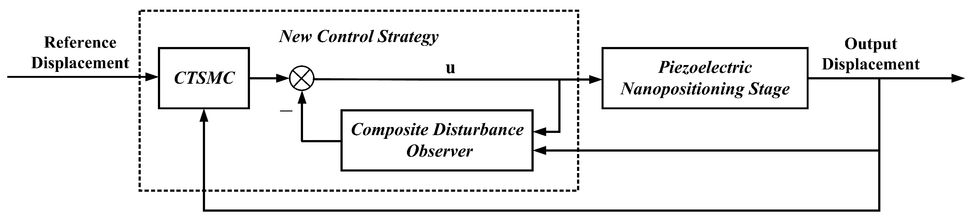
In order to improve the anti-disturbance performance of the piezoelectric nanopositioning stage system and the accuracy of position tracking, a new control strategy is designed. The design process of the control method can be described as follows: a continuous terminal sliding mode controller is designed to eliminate chattering and achieve finite time convergence, while a composite disturbance observer is designed to estimate the periodic and aperiodic disturbances in the system at the same time; then, the estimated value of the lumped disturbance is introduced into the controller to compensate for the disturbance of the system. Finally, the design of the composite controller is completed. The control block diagram is shown in Figure 1.

3.1. Composite Disturbance Observer Design

Assumption 2.

The lumped disturbance d satisfies that d is bounded, there exists a $K_1$ constant that satisfies $K_1\ge \left|\dot{d}\right|$, and d consists of aperiodic disturbance $d_{ap}$ and periodic disturbance $d_p$. $d_{ap}$ is a slow-varying and bounded disturbance, while $d_p$ is a sinusoidal disturbance, and its frequency is known.

Define the aperiodic disturbance $d_{ap}$ and the periodic disturbance $d_p$ as two augmented states, $x_3=d_{ap}$ and $x_4=d_p$; at the same time, another state $x_5$ is introduced to satisfy ${\dot{x}}_4=\omega x_5$. Then, three new states can be obtained as follows:

$$\left\{\begin{array}{c}d=d_{ap}+d_p=x_3+x_4,\hfill \\ x_4=Asin\left(\omega t+\phi \right),\hfill \\ x_5=Acos\left(\omega t+\phi \right).\hfill \end{array}\right.$$

(23)

System (2) obtains an extended state-space model as follows:

$$\left\{\begin{array}{c}{\dot{x}}_1=x_2,\hfill \\ {\dot{x}}_2=a_1{x}_1+a_2{x}_2+x_3+x{}_4+b_{0}u,\hfill \\ {\dot{x}}_3={\dot{d}}_{ap},\hfill \\ {\dot{x}}_4=\omega x_5,\hfill \\ {\dot{x}}_5=-\omega x_4,\hfill \\ y=x_1.\hfill \end{array}\right.$$

(24)

Then, the composite disturbance observer for system (24) is designed as follows:

$$\left\{\begin{array}{c}{\dot{\widehat{x}}}_1={\widehat{x}}_2-l_1\left({\widehat{x}}_1-x_1\right),\hfill \\ {\dot{\widehat{x}}}_2=a_1{\widehat{x}}_1+a_2{\widehat{x}}_2+{\widehat{x}}_3+{\widehat{x}}_4+b_{0}u-l_2\left({\widehat{x}}_1-x_1\right),\hfill \\ {\dot{\widehat{x}}}_3=-l_3\left({\widehat{x}}_1-x_1\right),\hfill \\ {\dot{\widehat{x}}}_4=\omega {\widehat{x}}_5-l_4\left({\widehat{x}}_1-x_1\right),\hfill \\ {\dot{\widehat{x}}}_5=-\omega {\widehat{x}}_4-l_5\left({\widehat{x}}_1-x_1\right),\hfill \\ \widehat{y}={\widehat{x}}_1.\hfill \end{array}\right.$$

(25)

Similar to Equation (12), the estimation error is defined as $e_i=x_i-{\widehat{x}}_i,i=1,\cdots ,5$, and the following can be obtained:

$$\left[\begin{array}{c}{\dot{e}}_1\hfill \\ {\dot{e}}_2\hfill \\ {\dot{e}}_3\hfill \\ {\dot{e}}_4\hfill \\ {\dot{e}}_5\hfill \end{array}\right]=\underset{\mathsf{\Theta }}{\underbrace{\left[\begin{array}{ccccc}-l_1& 1& 0& 0& 0\\ -l_2+a_1& a_2& 1& 1& 0\\ -l_3& 0& 0& 0& 0\\ -l_4& 0& 0& 0& \omega \\ -l_5& 0& 0& -\omega & 0\end{array}\right]}}\left[\begin{array}{c}{e}_1\\ e_2\\ e_3\\ e_4\\ e_5\end{array}\right]+\left[\begin{array}{c}0\\ 0\\ 1\\ 0\\ 0\end{array}\right]{\dot{d}}_{ap},$$

(26)

where $l_1$, $l_2$, $l_3$, $l_4$ and $l_5$ are parameters to be designed such that the matrix $\mathsf{\Theta }$ is a Hurwitz matrix. Then, under Assumption 2 and Lemma 2, the estimation error converges to zero asymptotically.

3.2. Continuous Terminal Sliding Mode Control Design

The control goal is to enforce the position tracking error to zero, which ensures that the output position $x_1$ tracks the given reference signal $x_r$. The tracking error is defined as follows:

$$e_t=x_r-x_1.$$

(27)

Taking the derivative and the second derivative of the tracking error, then substituting Equation (2) into it, we obtain the following:

$$\left\{\begin{array}{c}{\dot{e}}_t={\dot{x}}_r-{\dot{x}}_1,\hfill \\ {\ddot{e}}_t={\ddot{x}}_r-a_1\left(x_r-e_t\right)-a_2\left({\dot{x}}_r-{\dot{e}}_t\right)-b_{0}u-d.\hfill \end{array}\right.$$

(28)

Design the sliding surface as follows [20]:

$$s={\ddot{e}}_t+c_2\mathrm{sgn}\left({\dot{e}}_t\right){\left|{\dot{e}}_t\right|}^{{\alpha }_2}+c_1\mathrm{sgn}\left(e_t\right){\left|e_t\right|}^{{\alpha }_1},$$

(29)

where $0<{\alpha }_1<1,0<{\alpha }_2<1$, $c_1>0$, $c_2>0$ and $c_1$, $c_2$ are control parameters to be designed, and $\mathrm{sgn}$ is the standard symbolic function.

The CTSMC can be designed as follows:

$$u=b_0^{-1}\left(u_1+u_2\right),$$

(30)

$$u_1={\ddot{x}}_r-a_1\left(x_r-e_t\right)-a_2\left({\dot{x}}_r-{\dot{e}}_t\right)+c_2\mathrm{sgn}\left({\dot{e}}_t\right){\left|{\dot{e}}_t\right|}^{{\alpha }_2}+c_1\mathrm{sgn}\left(e_t\right){\left|e_t\right|}^{{\alpha }_1},$$

(31)

$$u_2=K{\int }_0^t\mathrm{sgn}\left(s\right)d\tau .$$

(32)

where $K>0$ and K is the gain of the controller.

Remark 1.

A method is proposed in [20] for calculating $\mathrm{sgn}\left(s\right)$, when the acceleration signal cannot be obtained directly.

Theorem 2.

Under Assumption 2 and the control law Equations (30)–(32), the error of the system will converge to zero in finite time if the gain satisfies $K>K_1$.

Proof of Theorem 2.

Considering Equation (28), the sliding surface (29) can be described as follows:

$$\begin{array}{c}s={\ddot{x}}_r-a_1\left(x_r-e_t\right)-a_2\left({\dot{x}}_r-{\dot{e}}_t\right)-\left(u_1+u_2\right)-d\hfill \\ +c_2\mathrm{sgn}\left({\dot{e}}_t\right){\left|{\dot{e}}_t\right|}^{{\alpha }_2}+c_1\mathrm{sgn}\left(e_t\right){\left|e_t\right|}^{{\alpha }_1}.\hfill \end{array}$$

(33)

Taking into account Equations (30) and (32)–(34), we can obtain the following:

$$s=-u_2-d.$$

(34)

Choosing the Lyapunov function as Equation (16), then taking the derivative of Equation (34), we have the following:

$$\dot{s}=-K\mathrm{sgn}\left(s\right)-\dot{d}.$$

(35)

Based on Assumption 2, the derivative of the Lyapunov function is as follows:

$$\begin{array}{c}\dot{V}=s\dot{s}=-K\left|s\right|-\dot{d}s\hfill \\ \le -K\left|s\right|+\left|\dot{d}s\right|\hfill \\ =-\left(K-\left|\dot{d}\right|\right)\left|s\right|\hfill \\ \le -\left(K-K_1\right)\left|s\right|\hfill \\ =-\sqrt{2}\left(K-K_1\right)V^{\frac{1}{2}}.\hfill \end{array}$$

(36)

Known from the analysis, when K satisfies $K>K_1$, the system states will reach the defined sliding surface $s=0$ in finite time.

This completes the proof. □

3.3. Composite Control Structure

A composite control structure based on the composite disturbance observer and CTSMC for the piezoelectric nanopositioning stage can be designed as follows:

$$\widehat{d}={\widehat{x}}_3+{\widehat{x}}_4,$$

(37)

$$s=-u_2-d.$$

(38)

$$u_1={\ddot{x}}_r-a_1\left(x_r-e_t\right)-a_2\left({\dot{x}}_r-{\dot{e}}_t\right)+c_2\mathrm{sgn}\left({\dot{e}}_t\right){\left|{\dot{e}}_t\right|}^{{\alpha }_2}+c_1\mathrm{sgn}\left(e_t\right){\left|e_t\right|}^{{\alpha }_1},$$

(39)

$$u_2=K{\int }_0^t\mathrm{sgn}\left(s\right)d\tau .$$

(40)

where $0<{\alpha }_1<1,0<{\alpha }_2<1$, $c_1>0$, $c_2>0$ and $c_1$, $c_2$ are control parameters to be designed, and $\mathrm{sgn}$ is the standard symbolic function.

The estimation of the lump disturbance is defined as $\widehat{d}$, and $\widehat{d}$ is used for compensation in addition to the CTSMC feedback part in order to reduce the steady-state fluctuation and tune down the gain of the CTSMC. The disturbance estimation error is defined as follows:

$$e_d=d-\widehat{d}.$$

(41)

Assumption 3.

The derivative of $e_d$ is bounded, and there exists a constant $K_2$ that satisfies $K_2\ge \left|{\dot{e}}_d\right|$.

Theorem 3.

Under Assumption 3 and the control law Equations (38)–(40), the error of the system will converge to zero in finite time if the gain satisfies $K>K_2$.

Proof of Theorem 3.

Considering Equation (24), the sliding surface can be described as follows:

$$\begin{array}{c}s={\ddot{x}}_r-a_1\left(x_r-e_t\right)-a_2\left({\dot{x}}_r-{\dot{e}}_t\right)-\left(u_1+u_2-\widehat{d}\right)-d\hfill \\ +c_2\mathrm{sgn}\left({\dot{e}}_t\right){\left|{\dot{e}}_t\right|}^{{\alpha }_2}+c_1\mathrm{sgn}\left(e_t\right){\left|e_t\right|}^{{\alpha }_1},\hfill \end{array}$$

(42)

$$s=-u_2-e_d.$$

(43)

Choosing the Lyapunov function as Equation (15), then taking the derivative of Equation (43), we obtain the following:

$$\dot{s}=-K\mathrm{sgn}\left(s\right)-{\dot{e}}_d.$$

(44)

Based on Assumption 2, the derivative of the Lyapunov function is as follows:

$$\begin{array}{c}\dot{V}=s\dot{s}=-K\left|s\right|-{\dot{e}}_{d}s\hfill \\ \le -K\left|s\right|+\left|{\dot{e}}_{d}s\right|\hfill \\ =-\left(K-\left|{\dot{e}}_d\right|\right)\left|s\right|\hfill \\ \le -\left(K-K_2\right)\left|s\right|\hfill \\ =-\sqrt{2}\left(K-K_2\right)V^{\frac{1}{2}}.\hfill \end{array}$$

(45)

Known from the analysis, when K satisfies: $K>K_2$ the system states will reach the defined sliding surface in finite time.

When $s=0$, the following equation can be obtained:

$$s={\ddot{e}}_t+c_2\mathrm{sgn}\left({\dot{e}}_t\right){\left|{\dot{e}}_t\right|}^{{\alpha }_2}+c_1\mathrm{sgn}\left(e_t\right){\left|e_t\right|}^{{\alpha }_1}=0.$$

(46)

Therefore, considering $c_1>0$ and $c_2>0$, the tracking error of the system will converge to zero along the sliding surface in finite time.

This completes the proof. □

4. Simulation Results and Experimental Tests

4.1. Experimental Setup and Model Identification

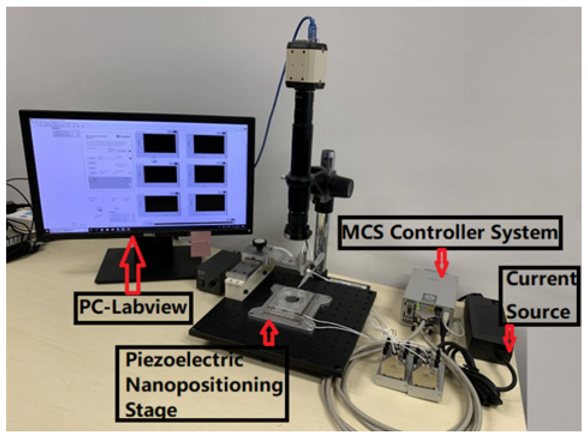
The experimental setup is shown in Figure 2. The piezoelectric nanopositioning stage (model: SLC1780, from SmarAct Inc., Oldenburg, Germany) is equipped with a linear slide, which is controlled by MCS2 (SmarAct Modular Control System 2). The piezoelectric nanopositioning stage travels approximately 51 mm. The MSC2 controller is equipped with a USB interface and can be controlled by Labview running on a PC. The positioners are equipped with integrated sensors, which deliver the digitized data to the main controller.

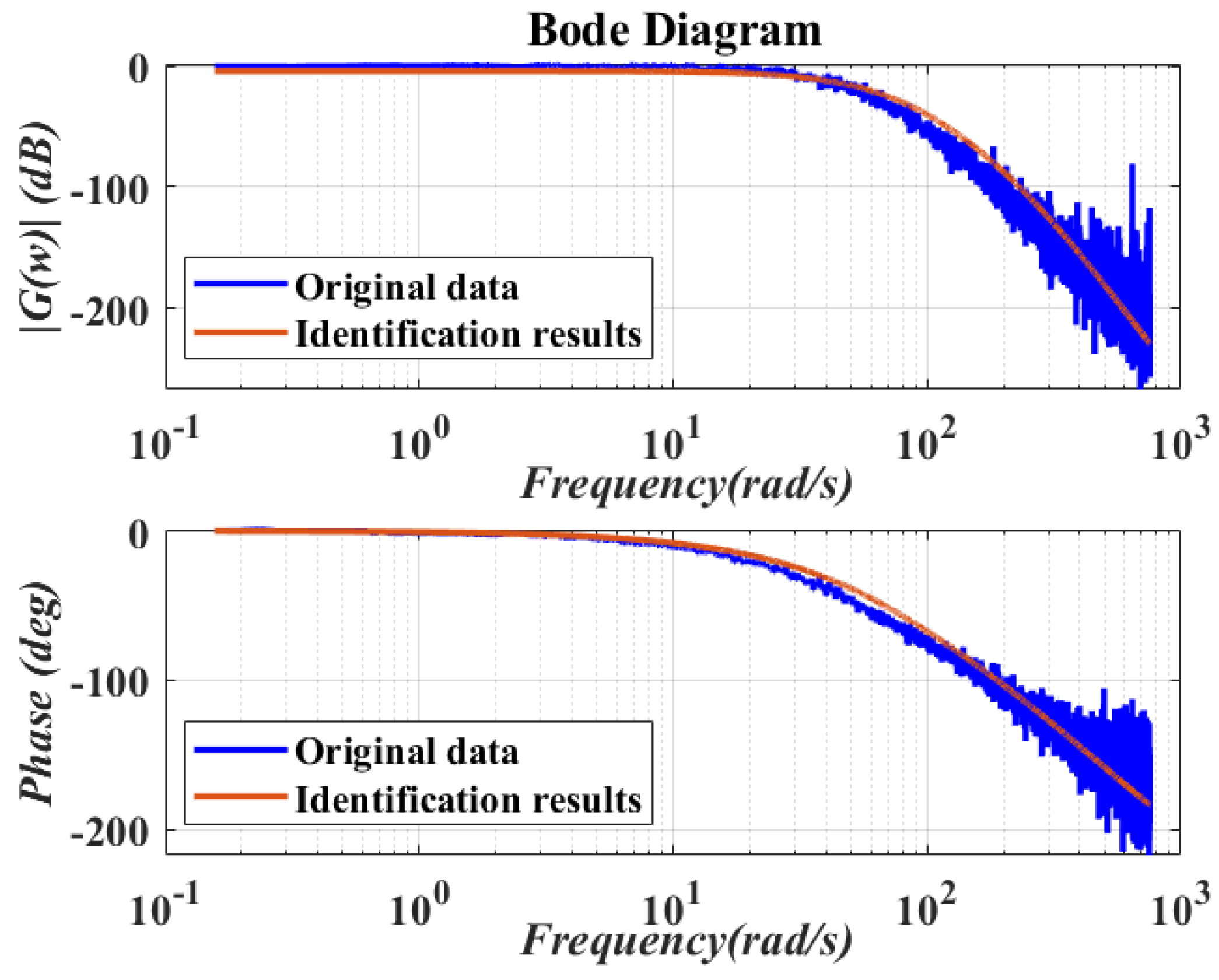
Under the voltage drive, the piezoelectric nanopositioning stage has a small positioning distance, and there is an approximate linear relationship between the input and output. To achieve the linear model, setting the scan velocity to a fixed value, we then input the Chrip signal to the move value module, where the amplitude is 10%, the frequency is 0.02–120 Hz, and the sampling frequency is 100 Hz.

According to Equation (1), the piezoelectric nanopositioning stage is a second-order system, so the system transfer function to be identified is also preset as second-order to identify the parameters of the system.

Figure 3 shows the frequency responses obtained from the experimental data and the identified model. The parameters of the linear second-order system can be identified by the least squares method:

$$G\left(s\right)=\frac{\mathrm{153,700}}{s^2+72.75s+1315}.$$

(47)

By comparing the coefficients of Equations (2) and (47), it can be seen that $a_1=-1315$, $a_2=-72.75$ and $b_0$ = 153,700, respectively.

4.2. Simulation Results

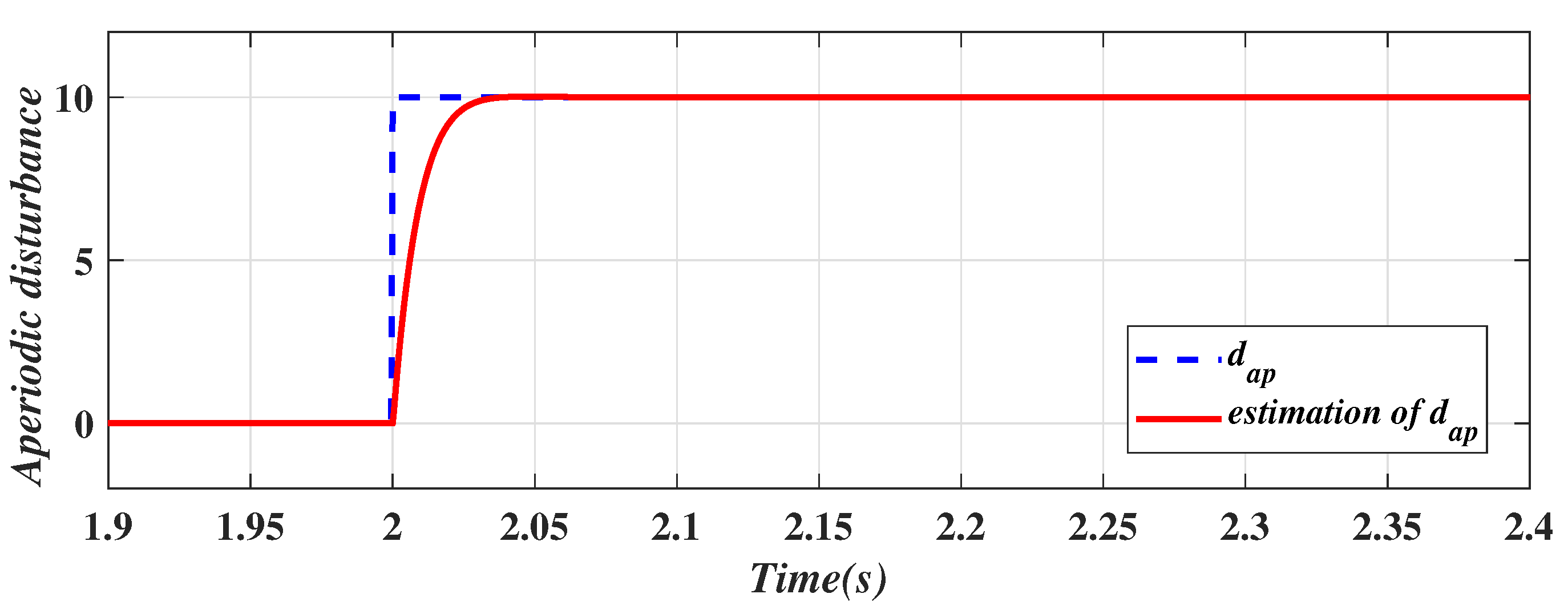
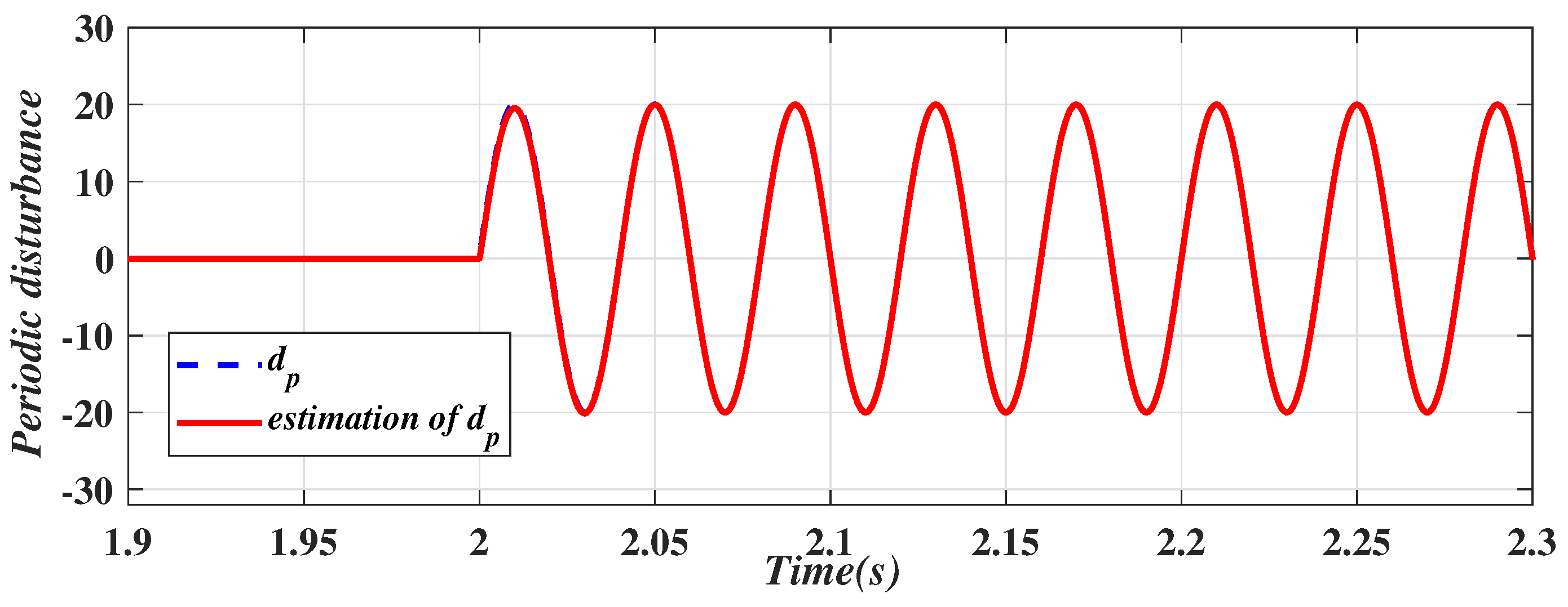
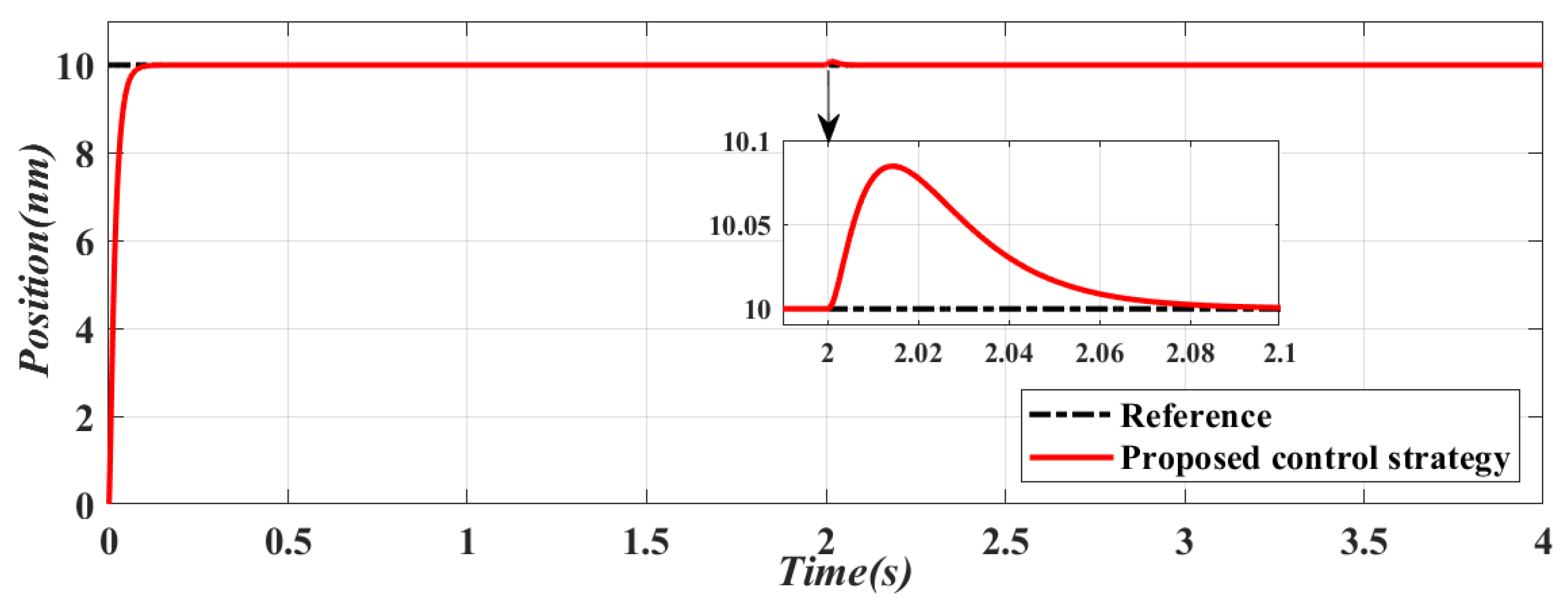
Simulations based on MATLAB are carried out to verify the performance of the proposed control strategy, especially in tracking ability, estimating and rejecting disturbance. In the simulation, the reference signal is set as a constant signal with the value of 10 nm (10,000 pm). In order to demonstrate the effectiveness of disturbance rejection, a lumped disturbance (including aperiodic disturbance and periodic disturbance) is added to the control channel at 2 s. The value of aperiodic disturbance is 10, while the amplitude of the periodic disturbance is 20, and the frequency of the periodic disturbance is 50 Hz. According to Equations (22), (35) and (36), the parameters are selected as follows: $l_1$ = 80, $l_2$ = 800, $l_3$ = 1000, $l_4$ = 5000, $l_5$ = 10,000, $c_1=10$, $c_2=7$, ${\alpha }_1$ = 9/23, ${\alpha }_2$ = 9/16 and K = 100,000.

It can be seen in Figure 4 and Figure 5 that both aperiodic disturbance and periodic disturbance can be estimated accurately. Figure 6 shows that the output can still track the reference signal with the proposed method when there is a lumped disturbance at 2 s.

4.3. Experiment Results

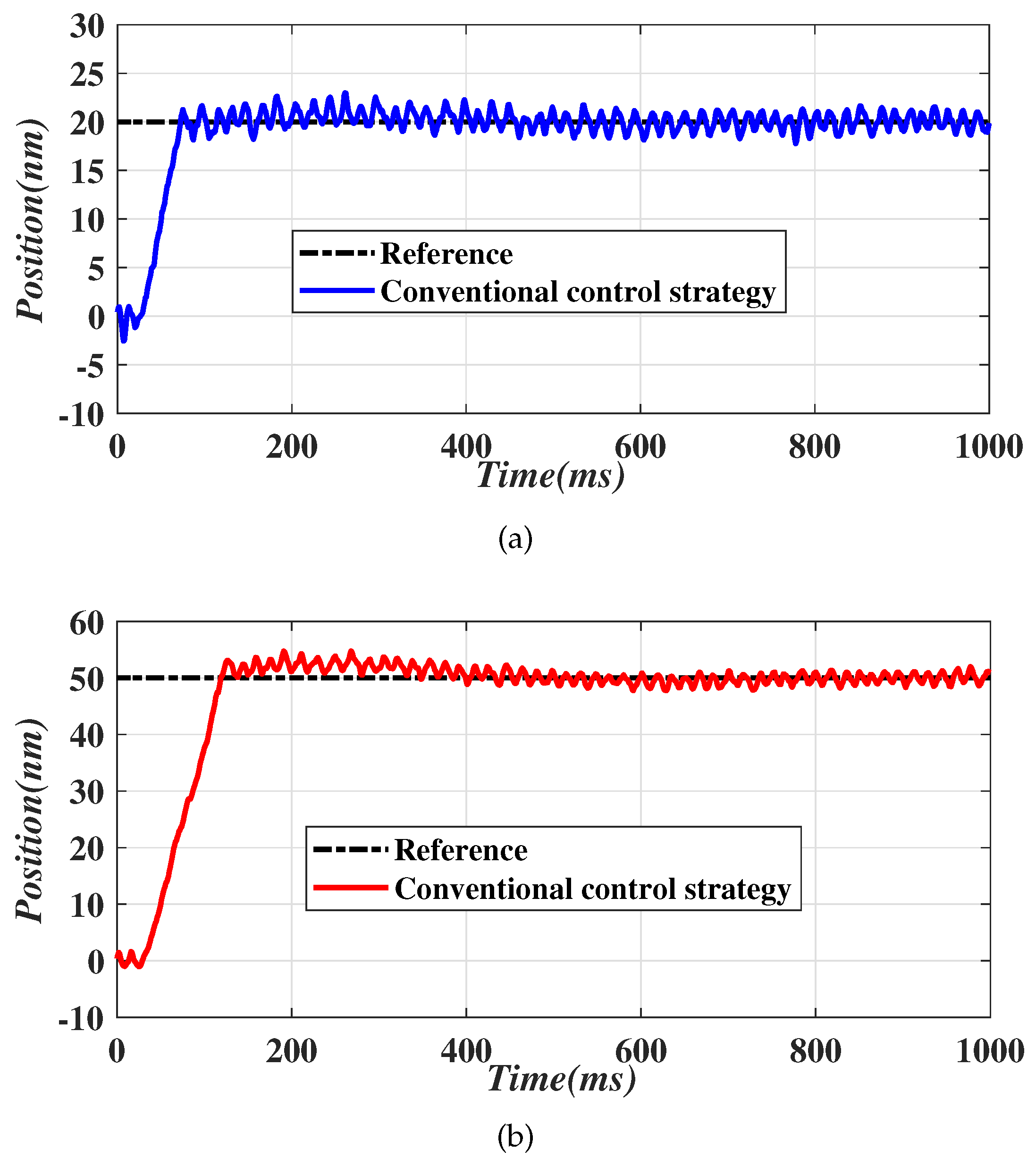
This experimental stage shown in Figure 2 is a part of the cell puncture composite system, whose main function is to transport the culture dishes containing cells to the designated location. Therefore, selecting the constant signal as the reference signal is more practical. In order to present the abundant experimental results, the author designed experiments to track two groups of constant signals (20 nm and 50 nm), respectively.

The conventional control designed in Section 2 is applied to the piezoelectric nanopositioning stage. Taking Equations (6), (15) and (18) into consideration, parameters are selected as follows: $l_1=78$, $l_2=563$, $l_3=62,500$, $c_1=60$, $c_2=10$ and K = 60,000.

Figure 7 shows the actual position trajectories, and Figure 8 shows the tracking error.

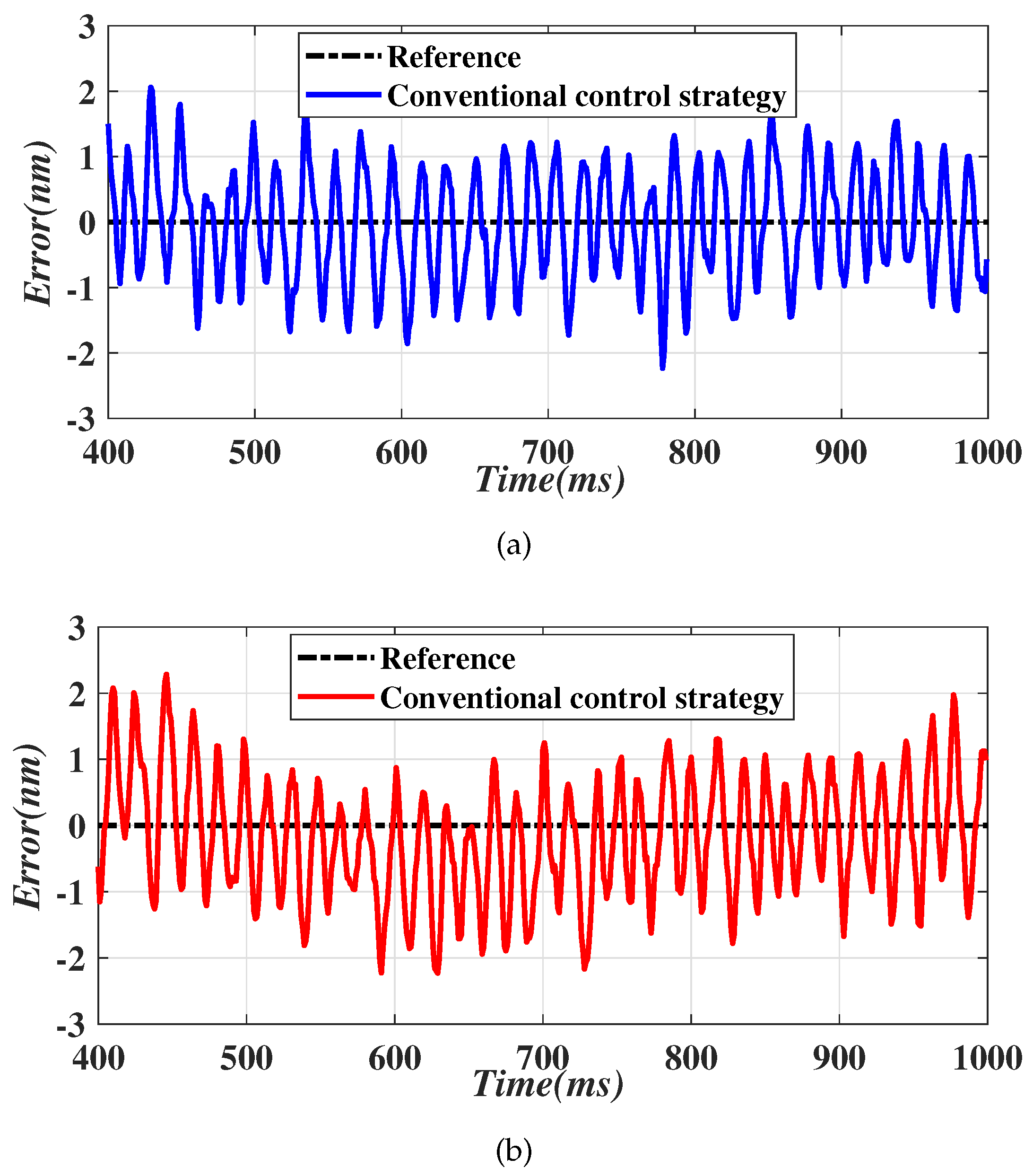
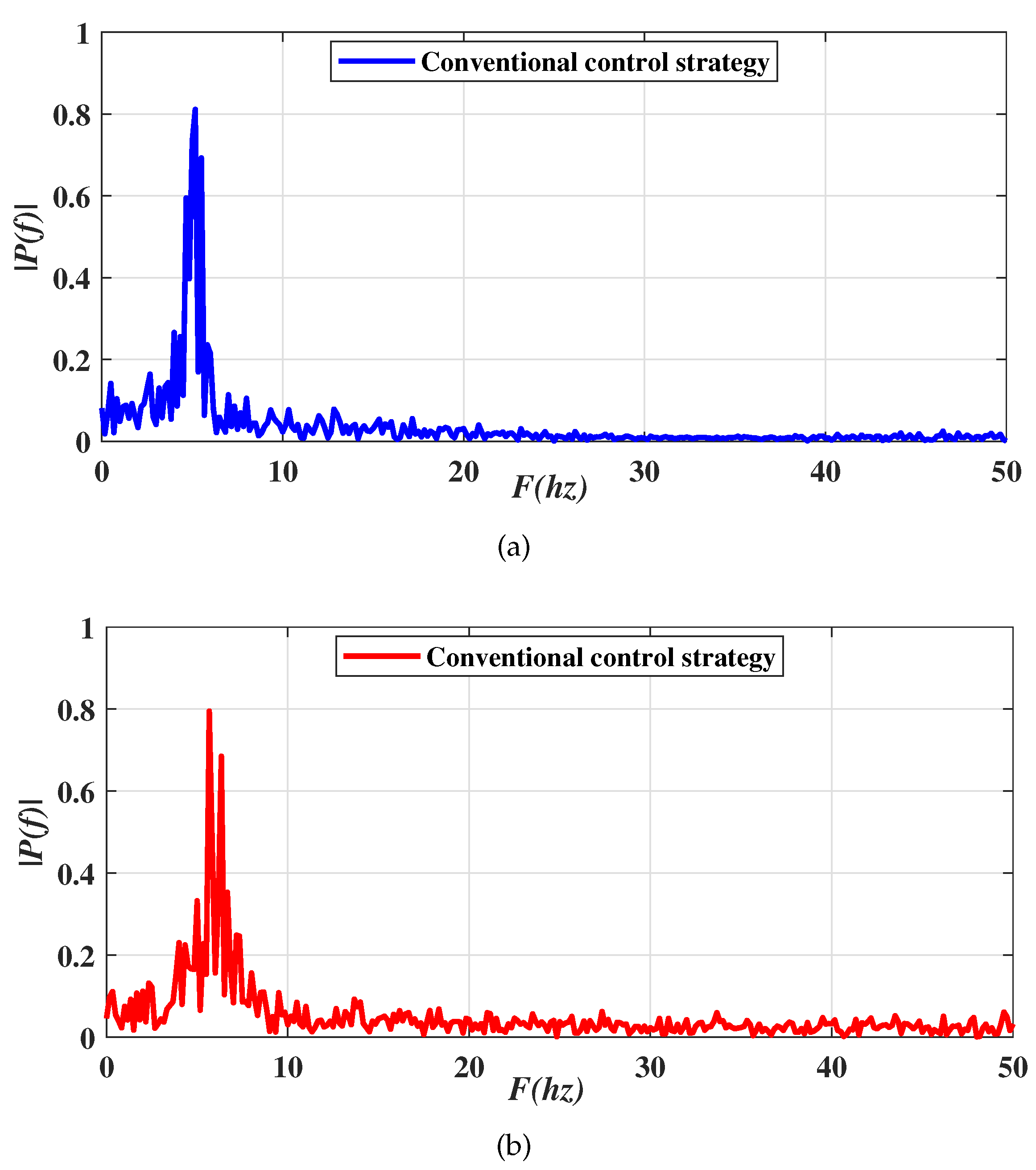
The steady-state errors shown in Figure 8 are to be transformed into one side Fourier transform. Figure 9 shows the transformed results. It is obvious that the frequency point at 5 Hz needs to be eliminated.

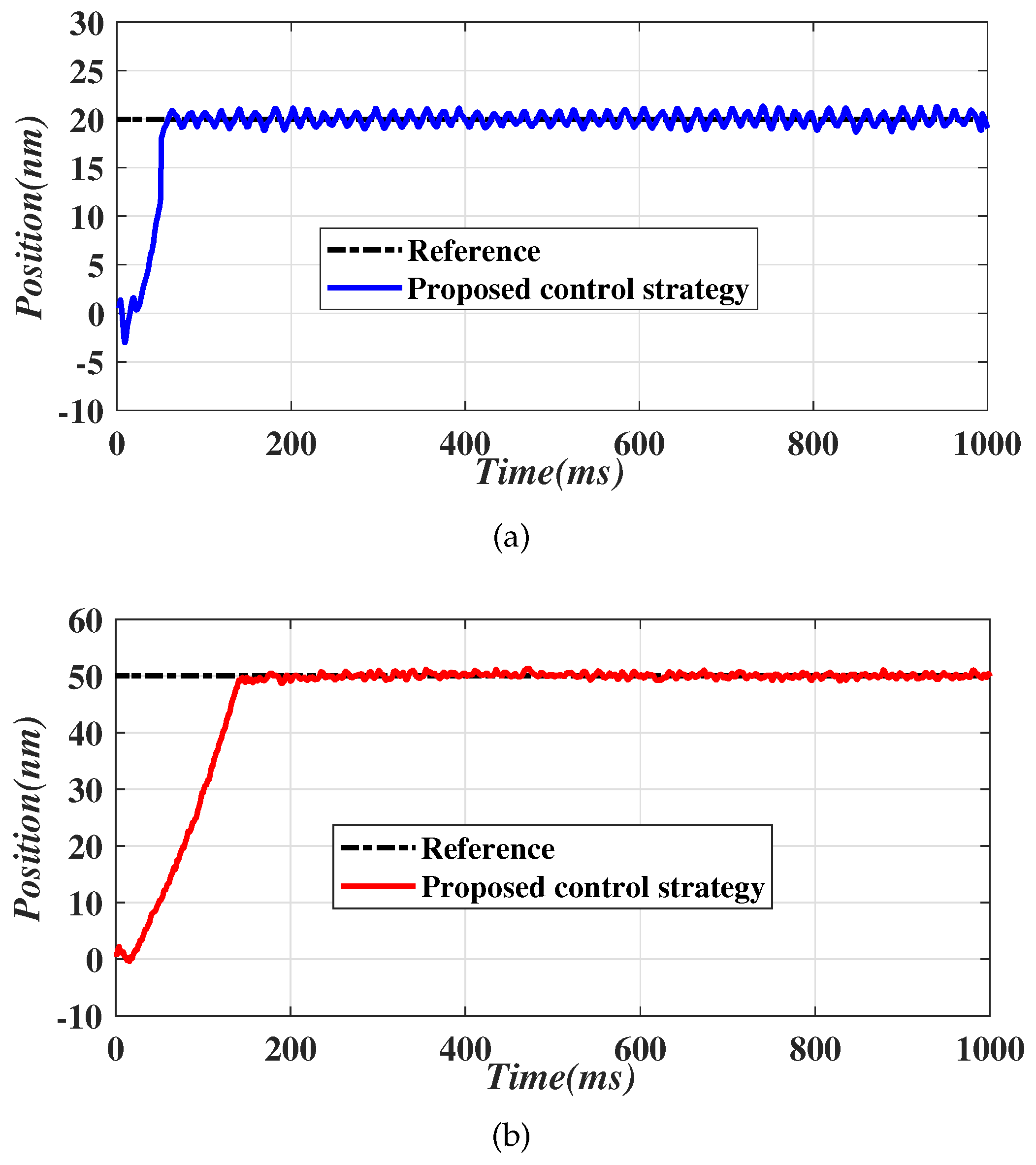
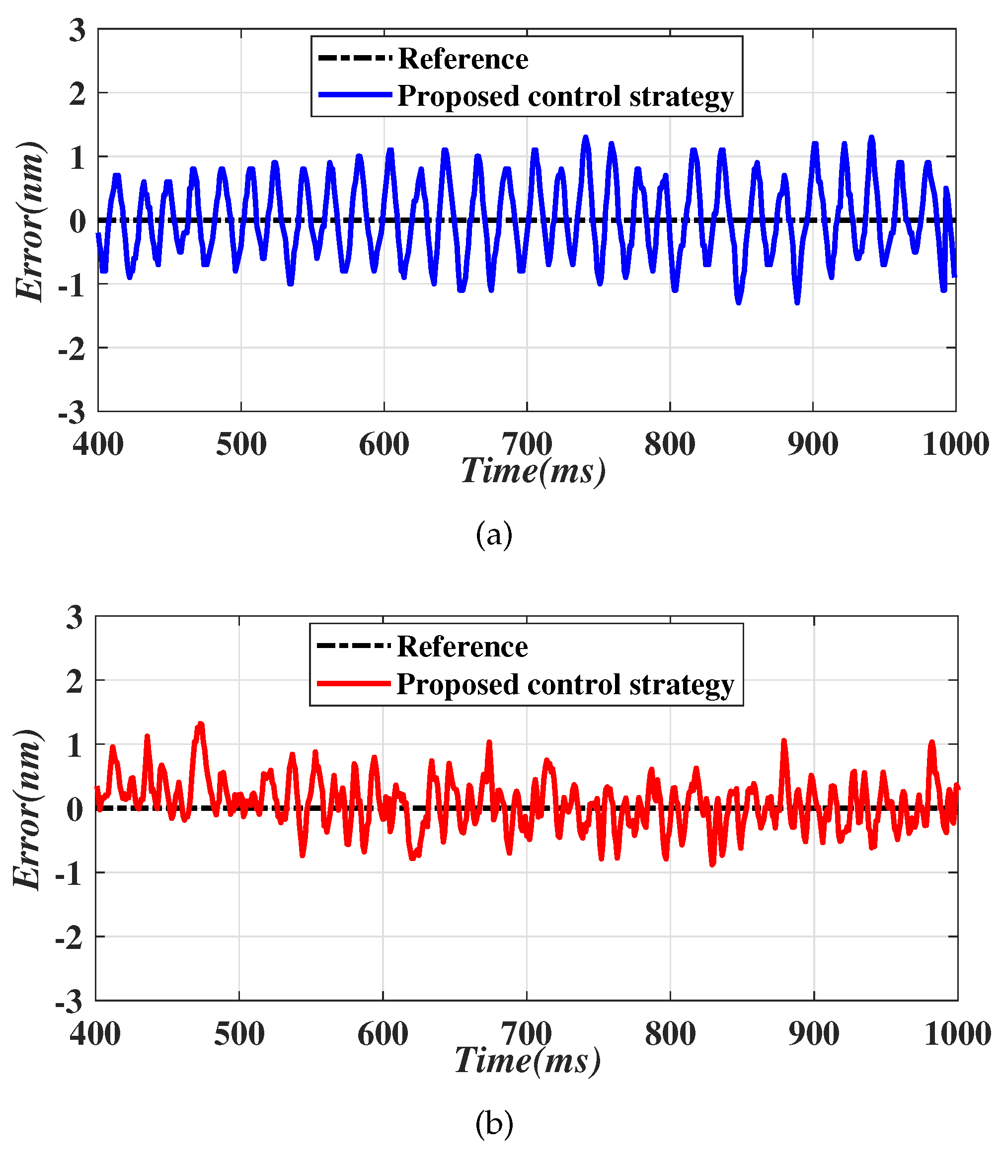
After obtaining the frequency of periodic disturbance, the proposed control strategy can be applied to the piezoelectric nanopositioning stage. The selection of the experimental parameters is similar to the simulation, except the control gain, which is chosen as K = 50,000. Figure 10 shows the actual position trajectories and Figure 11 shows the tracking error.

It can be seen from Figure 10 that the response of the system is faster in both working conditions. Obviously, Figure 11 shows that the steady-state error is controlled in the range of $\pm 1$ nm nearly, while the steady-state error of the conventional composite control strategy is in the range of $\pm 2$ nm. In fact, the position reading always fluctuates within $\pm 1$ nm without the reference signal and the control input, which is caused by the drift of the sensor.

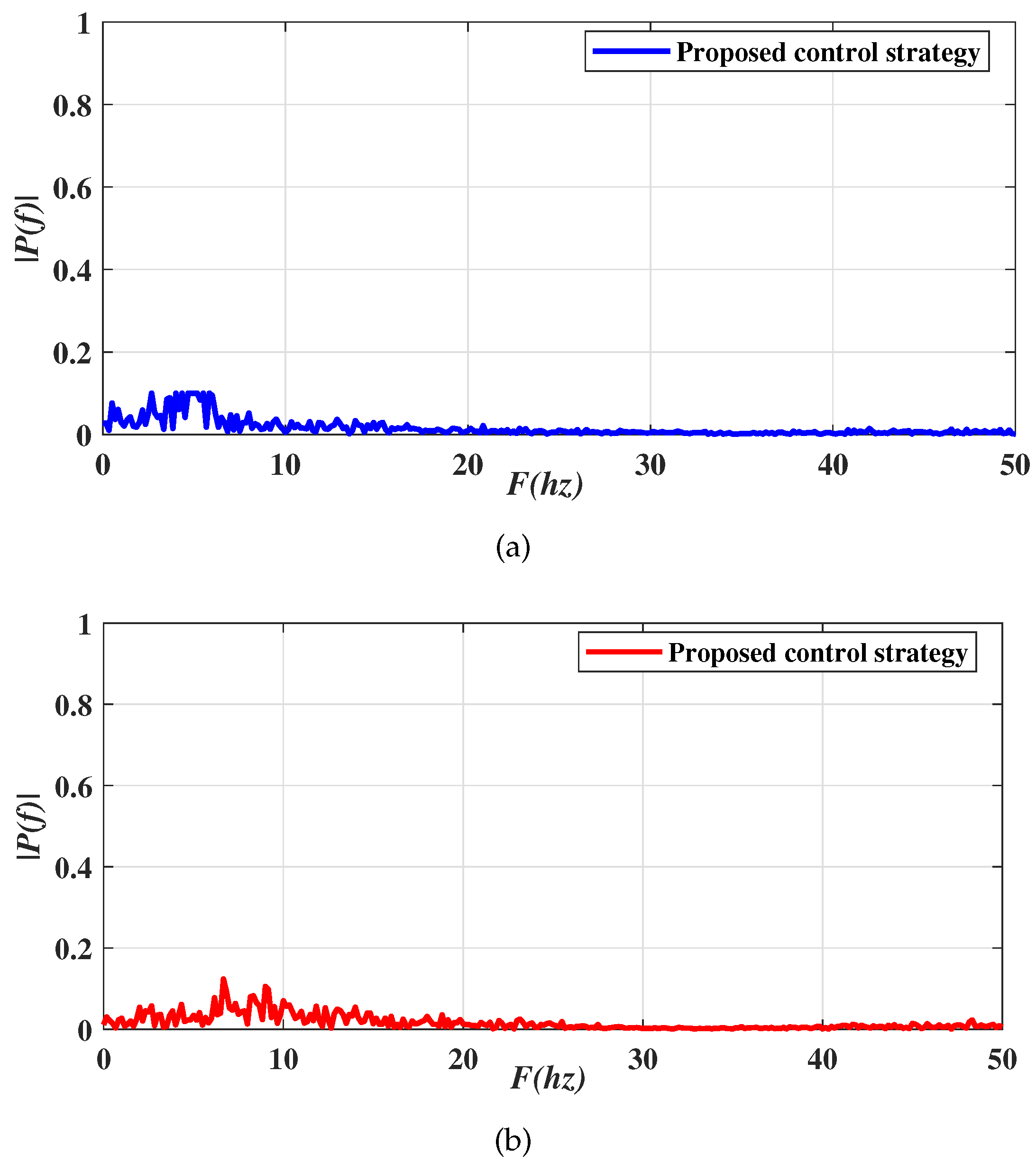
Similar to the above analysis, a single-sided Fourier transform is performed for the steady-state error. Figure 12 shows the transformed results; not only the frequency point at 5 Hz, but also the frequency points near 5 Hz obtain a significant decrease under the proposed composite control strategy.

5. Conclusions

As a single nonlinear control strategy can only improve the system performance in one aspect, it is difficult to meet the comprehensive performance index, and it is difficult to achieve the balance of anti-disturbance ability and dynamic and static performance. A composite control strategy based on composite disturbance observer and continuous terminal sliding mode control is proposed for piezoelectric nanopositioning stage in this paper. Continuous terminal sliding mode control is designed to eliminate the chattering phenomenon and ensure the tracking performance, and a composite disturbance observer is introduced to estimate both the periodic and aperiodic disturbances, simultaneously. The stability of the composite control strategy is demonstrated in theory based on the Lyapunov analysis. The effectiveness of the composite control strategy is verified by conducting experimental studies on a piezoelectric nanopositioning stage. The results show that the strategy is useful for the piezoelectric nanopositioning stage. In order to further improve the control performance and motion performance of the system, the author intends to combine the theoretical knowledge of fractional order controller [33,34] with the piezoelectric nanopositioning stage to complete the theoretical derivation and experimental verification.

References

- Vorbringer-Dorozhovets, N.; Hausotte, T.; Manske, E.; Shen, J.; Jaeger, G. Novel control scheme for a high-speed metrological scanning probe microscope. Meas. Sci. Technol. 2011, 22, 094012. [Google Scholar] [CrossRef]
- Yu, S.; Xie, M.; Manske, E.; Wu, H.; Ma, J.; Wang, R.; Kang, S. Design and control of a piezoactuated microfeed mechanism for cell injection. Int. J. Adv. Manuf. Technol. 2019, 105, 4941–4952. [Google Scholar] [CrossRef]
- Gu, G.; Zhu, L. An experimental comparison of proportional-integral, sliding mode, and robust adaptive control for piezo-actuated nanopositioning stages. Rev. Sci. Instrum. 2014, 85, 055112. [Google Scholar] [CrossRef] [Green Version]
- Li, C.; Ding, Y.; Gu, G.; Zhu, L. Damping control of piezo-actuated nanopositioning stages with recursive delayed position feedback. IEEE-ASME Trans. Mechatron. 2017, 22, 855–864. [Google Scholar] [CrossRef]
- Habineza, D.; Zouari, M.; Le, G.Y.; Rakotondrabe, M. Multivariable compensation of hysteresis, creep, badly damped vibration, and cross couplings in multiaxes piezoelectric actuators. IEEE Trans. Autom. Sci. Eng. 2018, 15, 1639–1653. [Google Scholar] [CrossRef] [Green Version]
- Gu, G.; Zhu, L.; Su, C.; Ding, H. Motion control of piezoelectric positioning stages: Modeling, controller design, and experimental evaluation. IEEE-ASME Trans. Mechatron. 2013, 18, 1459–1471. [Google Scholar] [CrossRef]
- Li, Y.; Xu, Q. Design and robust repetitive control of a new parallel-kinematic XY piezostage for micro/nanomanipulation. IEEE-ASME Trans. Mechatron. 2012, 17, 1120–1132. [Google Scholar] [CrossRef]
- Xu, Q. Piezoelectric nanopositioning control using second-order discrete-time terminal sliding-mode strategy. IEEE Trans. Ind. Electron. 2015, 12, 7738–7748. [Google Scholar] [CrossRef]
- Xu, Q. Digital sliding mode prediction control of piezoelectric micro/nanopositioning system. IEEE Trans. Control Syst. Technol. 2015, 23, 297–304. [Google Scholar] [CrossRef]
- Zhong, J.; Yao, B. Adaptive robust precision motion control of a piezoelectric positioning stage. IEEE Trans. Control Syst. Technol. 2008, 16, 1039–1046. [Google Scholar] [CrossRef] [Green Version]
- Li, S.; Wu, C.; Sun, Z. Design and implementation of clutch control for automotive transmissions using terminal-sliding-mode control and uncertainty observer. IEEE Trans. Veh. Technol. 2016, 65, 1890–1898. [Google Scholar] [CrossRef]
- Li, S.; Zhou, M.; Yu, X. Design and implementation of terminal sliding mode control method for PMSM speed regulation system. IEEE Trans. Ind. Inform. 2016, 9, 1879–1891. [Google Scholar] [CrossRef]
- Wang, H.; Li, S.; Lan, Q.; Zhao, Z.; Zhou, X. Continuous terminal sliding modecontrol with extended state observer for PMSM speed regulation system. Trans. Inst. Meas. Control 2017, 39, 1195–1204. [Google Scholar] [CrossRef]
- Xu, Q. Precision motion control of piezoelectric nanopositioning stage with chattering-free adaptive sliding mode control. J. Microelectromech. Syst. 2016, 25, 347–355. [Google Scholar] [CrossRef]
- Du, C.; Li, F.; Yang, C. An improved homogeneous polynomial approach for adaptive sliding-mode control of markov jump systems with actuator faults. IEEE Trans. Autom. Control 2020, 65, 955–969. [Google Scholar] [CrossRef]
- Zhang, X.; Lin, H. Backstepping fuzzy sliding mode control for the antiskid braking system of unmanned aerial vehicles. Electronics 2020, 9, 1731. [Google Scholar] [CrossRef]
- Bartoszewicz, A.; Adamiak, K. Discrete-time sliding-mode control with a desired switching variable generator. IEEE Trans. Autom. Control 2020, 65, 1807–1814. [Google Scholar] [CrossRef]
- Karamiz, A.; Tirandaz, H.; Barambones, O. Neural dynamic sliding mode control of nonlinear systems with both matched and mismatched uncertainties. J. Frankl. Inst.-Eng. Appl. Math. 2019, 356, 4577–4600. [Google Scholar]
- Xia, C.; Wang, X.; Li, S.; Chen, X. Improved integral sliding mode control methods for speed control of PMSM system. J. Int. J. Innov. Comput. Inf. Control 2011, 7, 1971–1982. [Google Scholar]
- Feng, Y.; Han, F.; Yu, X. Chattering free full-order sliding mode control. Automatica 2014, 50, 1310–1314. [Google Scholar] [CrossRef]
- Hou, H.; Yu, X.; Xu, L.; Rsetam, K.; Cao, Z. Chattering free full-order sliding mode control. IEEE Trans. Ind. Electron. 2020, 67, 5647–5656. [Google Scholar] [CrossRef]
- Mondal, S. Design of unknown input observer for nonlinear systems with time-varying delays. Intl. J. Dyn. Control 2015, 3, 448–456. [Google Scholar] [CrossRef]
- Yang, J.; Zheng, W.; Li, S.; Wu, B.; Cheng, M. Design of a prediction-accuracy-enhanced continuous-time MPC for sisturbed systems via a disturbance observer. IEEE Trans. Ind. Electron. 2015, 62, 5807–5816. [Google Scholar] [CrossRef]
- Chen, X.; Li, J.; Yang, J.; Li, S. A disturbance observer enhanced composite cascade control with experimental studies. Int. J. Control Autom. Syst. 2013, 11, 555–562. [Google Scholar] [CrossRef]
- Li, S.; Liu, Z. Adaptive speed control for permanent-magnet synchronous motor system with variations of load inertia. IEEE Trans. Ind. Electron. 2009, 56, 5807–5816. [Google Scholar]
- Han, J. From PID to active disturbance rejection control. IEEE Trans. Ind. Electron. 2009, 56, 900–906. [Google Scholar] [CrossRef]
- Yang, J.; Li, S.; Yu, X. Sliding-mode control for systems with mismatched uncertainties via a disturbance observer. IEEE Trans. Ind. Electron. 2013, 60, 160–169. [Google Scholar] [CrossRef]
- Chen, W.; Yang, J.; Guo, L.; Li, S. Disturbance-observer-based control and related methods-an overview. IEEE Trans. Ind. Electron. 2016, 63, 1083–1095. [Google Scholar] [CrossRef] [Green Version]
- Yan, Y.; Yang, J.; Sun, Z.; Zhang, C.; Li, S.; Yu, H. Robust speed regulation for PMSM servo system with multiple sources of disturbances via an augmented disturbance observer. IEEE-ASME Trans. Mechatron. 2018, 23, 769–780. [Google Scholar] [CrossRef]
- Wang, Z.; Yan, Y.; Yang, J.; Li, S.; Li, Q. Robust voltage regulation of a DC-AC inverter with load variations via a HDOBC approach. IEEE Trans. Circuits Syst. II 2019, 66, 1172–1176. [Google Scholar] [CrossRef]
- Sayem, A.; Cao, Z.; Man, Z. Model free ESO-based repetitive control for rejecting periodic and aperiodic disturbances. IEEE Trans. Ind. Electron. 2017, 64, 3433–3441. [Google Scholar] [CrossRef]
- Khalil, H. Nonlinear Systems, 3rd ed.; Prentice Hall: Hoboken, NJ, USA, 2002; pp. 110–125. [Google Scholar]
- Sami, I.; Ullah, S.; Ullah, N.; Ro, J.-S. Sensorless fractional order composite sliding mode control design for wind generation system. ISA Trans. 2021, 111, 275–289. [Google Scholar] [CrossRef] [PubMed]
- Sami, I.; Ullah, S.; Ali, Z.; Ullah, N.; Ro, J.-S. A super twisting fractional order terminal sliding mode control for DFIG-based wind energy conversion system. Energies 2020, 13, 2158. [Google Scholar] [CrossRef]
Figure 1.
Control block diagram of piezoelectric nanopositioning stage system.
Figure 2.
Experimental setup of piezoelectric nanopositioning stage system.
Figure 3.
Frequency responses obtained by original data and identification results.
Figure 4.
Aperiodic disturbance and estimation of aperiodic disturbance.
Figure 5.
Periodic disturbance and estimation of periodic disturbance.
Figure 6.
Tracking curve for reference displacement.
Figure 7.
Tracking curve for reference displacement. (a) Reference = 20 nm. (b) Reference = 50 nm.
Figure 8.
Tracking error under the conventional composite control strategy. (a) Reference = 20 nm. (b) Reference = 50 nm.
Figure 9.
Transformed results of tracking error under conventional composite control strategy. (a) Reference = 20 nm. (b) Reference = 50 nm.
Figure 10.
Tracking curve under the proposed composite control strategy. (a) Reference = 20 nm. (b) Reference = 50 nm.
Figure 11.
Tracking error under the proposed composite control strategy. (a) Reference = 20 nm. (b) Reference = 50 nm.
Figure 12.
Transformed result of tracking error under theproposed composite control strategy. (a) Reference = 20 nm. (b) Reference = 50 nm.
Publisher’s Note: MDPI stays neutral with regard to jurisdictional claims in published maps and institutional affiliations. |
© 2021 by the authors. Licensee MDPI, Basel, Switzerland. This article is an open access article distributed under the terms and conditions of the Creative Commons Attribution (CC BY) license (https://creativecommons.org/licenses/by/4.0/).
Share and Cite
MDPI and ACS Style
Qiao, P.; Yang, J.; Dai, C.; Xiao, X. Design of Composite Disturbance Observer and Continuous Terminal Sliding Mode Control for Piezoelectric Nanopositioning Stage. Electronics 2021, 10, 2242. https://doi.org/10.3390/electronics10182242
AMA Style
Qiao P, Yang J, Dai C, Xiao X. Design of Composite Disturbance Observer and Continuous Terminal Sliding Mode Control for Piezoelectric Nanopositioning Stage. Electronics. 2021; 10(18):2242. https://doi.org/10.3390/electronics10182242
Chicago/Turabian StyleQiao, Pengyu, Jun Yang, Chen Dai, and Xi Xiao. 2021. "Design of Composite Disturbance Observer and Continuous Terminal Sliding Mode Control for Piezoelectric Nanopositioning Stage" Electronics 10, no. 18: 2242. https://doi.org/10.3390/electronics10182242
Note that from the first issue of 2016, this journal uses article numbers instead of page numbers. See further details here.