Design Optimization of Wearable Multiband Antenna Using Evolutionary Algorithm Tuned with Dipole Benchmark Problem

Abstract

In this paper we present the optimal design of wearable four band antenna that is suitable to work in the fifth-generation wireless systems as well as in cellular systems and in unlicensed bands. The design of the antenna relies on a careful study of optimization algorithms that are suitable for antenna design. We have proposed a benchmark problem to compare different optimization algorithms. It is the space of voltage standing wave ratio and the gain of dipole antenna that was identified for wide range of dipole length and radius. Using this pre-calculated data, we have tuned the parameters of optimization routine for optimal performance with our benchmark. After this, we optimized the geometry of four-band wearable antenna. In the optimization process, we used finite-difference time-domain method together with simplified model of human body. The antenna design was assessed with a fabricated prototype.

1. Introduction

Systems for wireless monitoring of human vital parameters have been intensively developed in recent years [1]. They find numerous applications in medicine for monitoring cardiac patients and convalescents [2]. Such systems are also used in sports medicine to monitor the parameters of training people [3]. Another application is the control of the working environment and people working in dangerous conditions [4]. In each of these applications, it is important to use an appropriate wireless data transmission technology. the bandwidth of which is matched to the amount of data sent in such a system. It is equally important that the data transmission technology is available in the assumed locations and enables the planned range of the system to be achieved.

The dynamic development of wireless communication systems has resulted in the development of many standards that coexist with each other in different frequency bands. In recent years, fifth generation systems (5G) have been introduced to the market, for which the 3.6 GHz band is currently used. At the same time, systems using the 1.8 GHz band such as LTE are still working. Wireless computer networks (WiFi) operating in the 2.4 GHz and 5.8 GHz bands are also very widespread, which enable the implementation of transmission systems independent of cellular network operators. In the case of people monitoring systems, networks of this type are particularly important because they provide the possibility of data transmission inside buildings where the range of cellular systems is often limited.

Due to the coexistence of various wireless communication technologies, it is possible to simultaneously use several systems for data transmission. This solution substantially improves the reliability of transmission because in the case of lack of coverage of one of the systems, it is possible to use another one [5]. In wireless systems designed for human monitoring, high certainty and reliability of transmission is required because the inability to send a message about the occurrence of anomalous medical parameters may pose a threat to the patient’s health.

In the article, we presented a design of a wearable antenna designed to work in a wireless patient monitoring system, which can use several transmission technologies. We assumed that the operating frequency range of such an antenna should cover the 1.8 GHz. 2.4 GHz. 3.6 GHz and 5.8 GHz bands. Thanks to this, the antenna can be used to work in the 5G, LTE, as well as WiFi and Bluetooth systems. An important design assumption is the use of thin-film laminate technology, thanks to which a flexible wearable antenna can be made, which minimally reduces the user’s comfort. For operational reasons, antennas of this type should be as small as possible so that it can be easily integrated with both the transmitter system and clothing. At the same time, the gain of such an antenna should be as large as possible, so that there is no need to use too much transmission power in the link, which would significantly reduce the battery life.

Due to numerous design requirements for the wearable multiband antenna, we used an automated optimization algorithm and electromagnetic analysis code taking into account the antenna model and a simplified human body model. Due to the fact that there are numerous optimization algorithms available, and they require proper selection of parameters. We have performed preliminary research on the evaluation of the properties of optimization algorithms. They were carried out with the use of a benchmark problem which was to design a rod dipole antenna.

2. Materials and Methods

2.1. Benchmark Problem

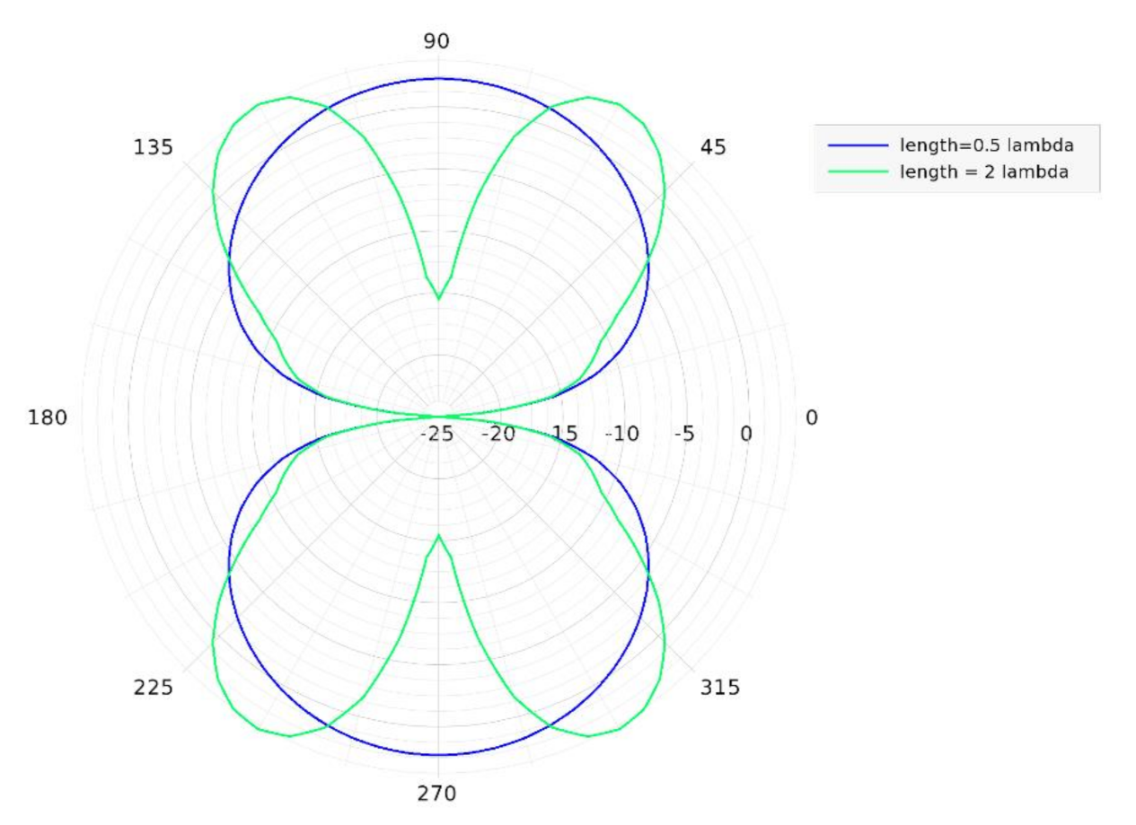
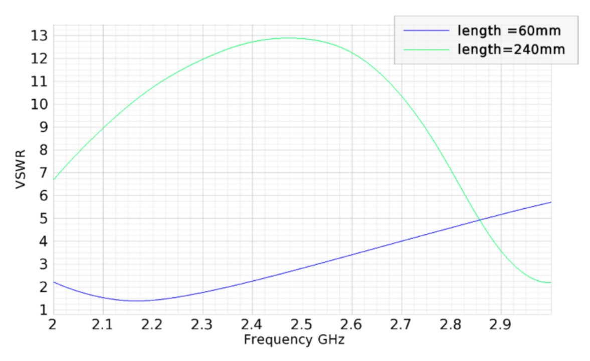
Dipole antenna is very simple radiating structure (presented in Figure 1). Of very well identified performance. Its electric properties depend on two design parameters: antenna length and antenna radius. In Figure 2 the radiation pattern of dipole with different length are presented. In Figure 3, the impedance matching of the dipoles varying in length is presented using for simplicity of comparison the Voltage Standing Wave Ratio (VSWR) with reference impedance equal to 50 Ω. It can be noted that the change in one parameter of this antenna significantly changes both radiation pattern and input impedance matching.

For a thin dipole that has radius r much smaller than length L, there is an analytical solution for antenna input impedance and gain [6]. In turn, for thick antennas in which radius is comparable to length, numerical methods have to be applied due to more complex antenna current distribution. Thanks to simple design of dipole antennae, it can be simulated with almost any full wave numerical method that is used nowadays in computational electromagnetics.

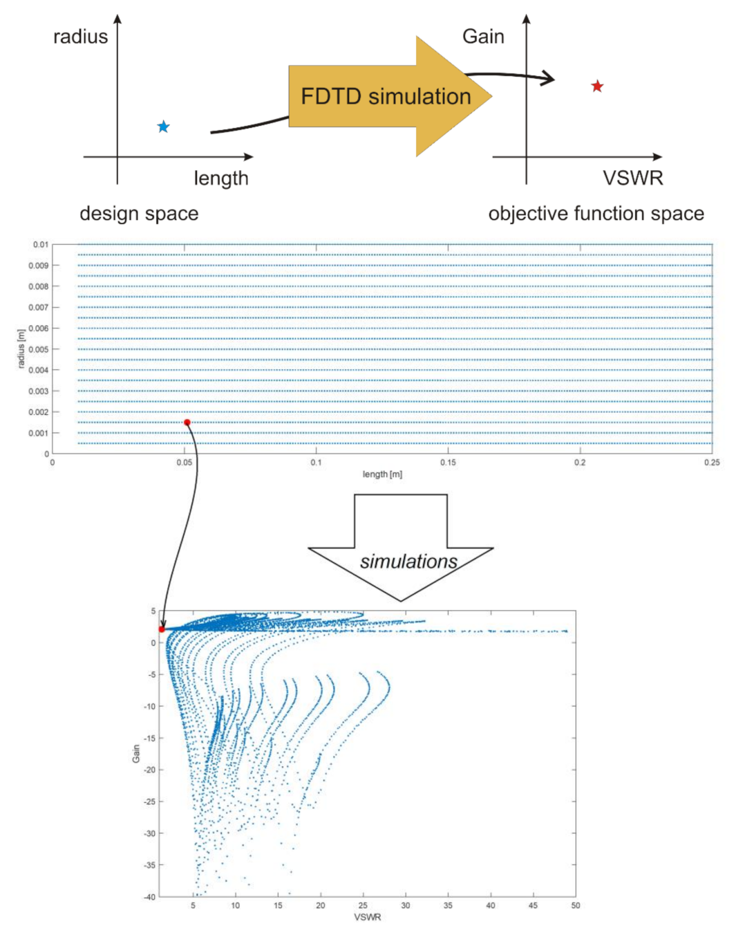
Due to this features we decided to use dipole as a benchmark for testing optimization algorithms. For this purpose, we have proposed the objective function (1) that has the value of dipole VSWR and gain G in the direction perpendicular to the antenna axis subject to dipole length L and radius r. for frequency of 2.5 GHz (wavelength λ = 0.12 m)

$$\left(VSWR.G\left(\theta =90°\right)\right)=f\left(r.L\right)$$

(1)

where f is a vectorial two-component function dependent on the two design variables.

The values of Equation (1) were obtained using full-wave simulations with finite-difference time-domain method (FDTD). We applied for this purpose Remcom Xfdtd software [7,8]. The design space (r.L) was searched in the wide range addressing thin structures as well as thick. The antenna radius varied in the range of 0.0005 m < r < 0.01 m with the step of 0.0005 m. Antenna length was scanned in the wide range: 0.01 m < L < 0.25 m with 0.001 m step. The length of dipole antennae varied from 0.083·λ to 2.083·λ. All combinations of radius and length gave rich set of 4820 points, for which VSWR and G(θ = 90°) is simulated. In Figure 4, the full design space is presented, as well as the majority of points in objective function components space (for this case, a few points are not shown due to the scaling effect).

The values of sampled function (1) were stored in a look-up table. We have used Matlab environment to create the function that implemented data search in the table. If the required value of {r.L} parameters was not matching the exact value of samples, then the closest values were identified and the output {VSWR.G} was calculated as an average of the values available for the closest arguments.

2.2. Algorithm Comparison—Single Objective

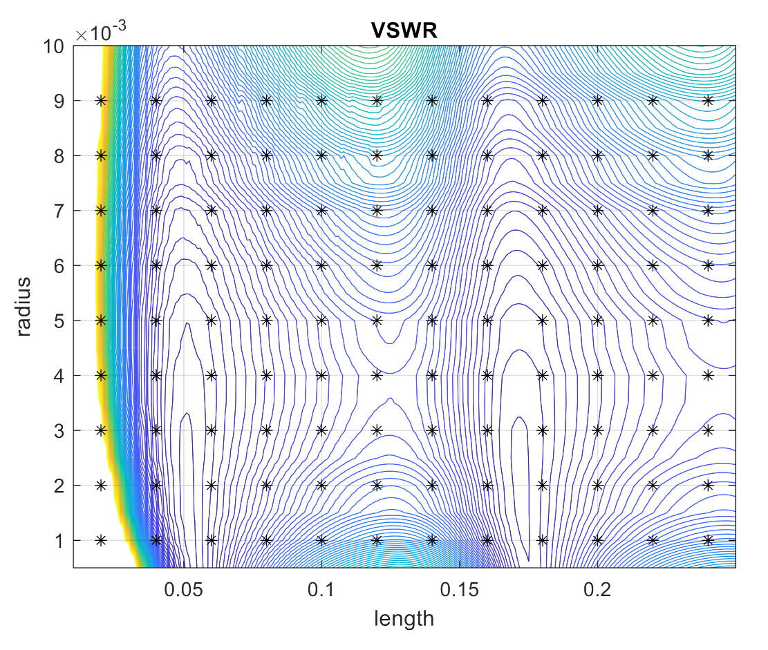
In the first stage of our research, we have exploited the benchmark problem to test in a comparative way the performance of algorithms that can be used for single objective optimization. Specifically, we used algorithms that are implemented in Matlab such as the Nelder-Mead simplex direct search [9,10], Interior point [11,12,13], and Quasi Newton [14,15]. We also used our own implementation of Powell algorithm of conjugate directions and also a single-objective evolutionary algorithm of the lowest order—EStra [16]. Each algorithm was tested with 108 runs using different starting points. In Figure 5, the set of starting points is presented in (r-L) design parameter space. In the same diagram, the values of VSWR are shown by means of contour lines.

Table 1. Performance of the optimization in the case of VSWR minimization for 108 starting points (O.F.—Objective Function).

nr	Method	Minimum Value of O.F.	Average Value of O.F.	Maximum Value of O.F.	Minimum Number of O.F. Calls	Average Number of O.F. Calls	Maximum Number of O.F. Calls
1	Nelder-Mead	1.32352	2.10497	8.25074	13	38	200
2	Interior point	1.39020	4.65605	27.46539	3	34.96296	67
3	Quasi-Newton (Matlab fminunc function)	2.22250	12.94491	159.88125	3	24.7	53
4	Powell	1.32352	1.81385	7.84942	200	530.37	2083
5	EStra	1.32352	1.66089	2.58385	41	48.5	67

presents the performance parameters of different optimization algorithms that were minimizing VSWR. In this case EStra algorithm had the best performance in terms of average and maximum value of objective function (VSWR) that was calculated over 108 final values identified from different starting points.

Table 2. Performance of the optimization in the case of Gain maximization (108 starting points).

nr	Method	Minimum Value of O.F.	Average Value of O.F.	Maximum Value of O.F.	Minimum Number of O.F. Calls	Average Number of O.F. Calls	Maximum Number of O.F. Calls
1	Nelder-Mead	−14.6865	1.71705	4.77681	15	56.80556	403
2	Interior point	−9.3953	1.77494	4.73644	3	35.9722	68
3	Quasi-Newton (Matlab fminunc)	−30.6766	−2.902	4.75	3	25.018	53
4	Powell	Inf	inf	4.77681	198	2551.129	19,804
5	EStra	3.7473	4.5014	4.7768	41	58.2037	97

presents the performance parameters of different optimization algorithms that were maximizing Gain. Also, the EStra algorithm has the best performance here in terms of average and minimum value of objective function (Gain) over different starting points. This is a good feature of the optimization algorithm that is not sensitive to starting point selection and gives solutions that are close to optimal.

2.3. Pareto-Inspired Evolutionary Optimization: P-EStra Algorithm

Eventually, a full multi-objective approach in terms of (VSWR.G) space was considered, without resorting to a scalar preference function like in Section 2.2.

In the literature, there are plenty of algorithms for local or global optimization: generally speaking, they can be categorized as belonging to the class of deterministic computing or evolutionary computing or nature-inspired computing; a few of them were specifically designed for multi-objective optimization purposes like, e.g., the popular NSGA-II [16]. In fact, the algorithmic paradigm offered by evolutionary computing is particularly suited for implementing the Pareto optimality criterion in the search for non-dominated solutions trading off two or more conflicting objectives. On the other hand, however, the major drawback of every algorithm of evolutionary computing is the substantial computational burden that is required. The cost issue is particularly important when the computation of the objective functions and constraint functions imply the solution of a field analysis problem by means of finite-element or finite-difference models in three dimensions, like it was in our case.

Moving from this background, a cost-effective algorithm based on a multiobjective (1 + 1)-evolution strategy (P-EStra) inspired by Pareto optimality theory was utilized [16]. The key concept is twofold: considering the design variables as random numbers characterized by mean values and standard deviations, on the one hand, and accepting a new solution according to the Pareto-like criterion of non-dominated solution, on the other hand.

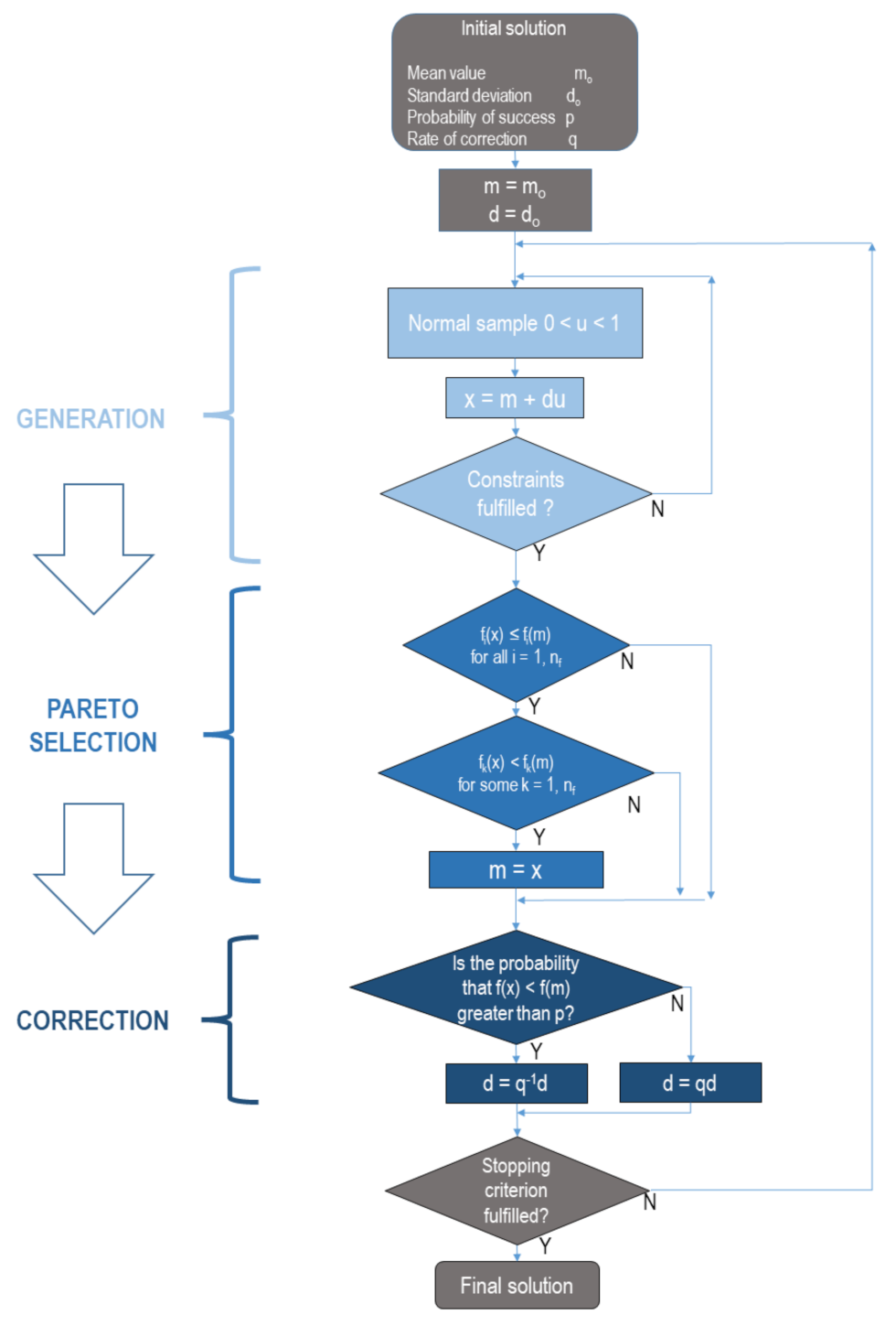
In more detail, the P-EStra algorithm is based on the following scheme: consider the design vector m at the current iteration, and the relevant vector d of standard deviation values; this means that d(k) is the standard deviation value of the k-th design variable whose mean value is m(k). At the subsequent iteration, a new design vector x is generated after perturbing the d vector by means of a normally distributed sample $u \in \left[0,1\right]$. and then the perturbation ud is added to the mean value m (parent solution); it turns out to be x = m + ud. This simple operation implements a principle of evolutionary computing: at this point in time, in fact, the offspring solution x is accepted if and only if it simultaneously improves all the objective functions, subject to the problem constraints; otherwise, the parent m is kept, and a new perturbation takes place. In other words, an offspring solution is selected if it is better, or at least non-worse, than the parent solution against all the m objective functions: this way, given an initial guess solution, there is a non-null probability that the optimization trajectory eventually converges to a point belonging to the Pareto optimal front.

Every algorithm of numerical optimization depends on a number of characteristic parameters, and P-EStra is no exception. The most important parameters that influence the performance of the algorithm are called p and q, respectively, in particular. p is the prescribed probability of successful iteration: an iteration is considered to be successful if the values of the objective functions improve with respect to the previous iteration (or, equivalently, if x is preferred to m). Accordingly, the ratio of the number of successful iterations to the total number of iterations is the effective probability p_e; in turn. q is the rate of correction the standard deviation d must undergo during the optimization.

As far as the convergence criterion is concerned, the following remark can be put forward: Vector d, which drives the search, undergoes a modification which is ruled by a randomized process. In fact, given the correction rate $q \in \left(0.1\right)$. considering the k-th iteration. $d_{k+1}=q^{-1}·d_k$ is set to force a larger standard deviation of Gaussian distribution associated with x in the next iteration; this happens when p_e > p in order to increase the exploration capability of the algorithm. In contrast. $d_{k+1}=q·d_k$ is set to force a smaller standard deviation of the Gaussian distribution in the next iteration; this happens when p_e < p in order to increase the exploitation capability of the algorithm. It appears that an appropriate tuning of p and q values is mandatory for a good performance of the algorithm; the issue is discussed in the subsequent Section 2.4.

P-EStra algorithm converges when the ratio of the largest value of the elements of the current standard deviation d vector to the corresponding element of the initial standard-deviation vector d_o is smaller than the prescribed search tolerance.

As far as initialization is concerned, the following remark can be put forward. Vector m is initialized as m_o, which contains the initial guess solution, and in turn, vector d is initialized as d_o and the value of its elements is proportional to the admissible range of the corresponding design variables.

Moreover, it is possible to a priori compute a rough estimation of the cost c of P-EStra algorithm by multiplying the following factors:

• c₀. the hardware-dependent time necessary to run a single solution of the direct problem associated to the optimization problem;
• n_i. the number of convergence iterations for a prescribed search accuracy;
• n_p. the number of evolving solutions (in our case. n_p = 1);
• n_f. the number of objective functions.

It turns out to be:

$$c\approx c_0·n_i·n_p·n_f$$

which gives a reasonable estimate of the computational budget to be allotted.

The principal flow-chart of the algorithm is shown in Figure 6.

Summing up, the evolutionary algorithm starts from a guess solution, which can be either user-supplied or randomly generated, iteratively originating a search trajectory driven by the concept of non-dominated solution, and eventually converges to a Pareto-optimal solution.

2.4. Algorithm Tuning—Bi-Objective Case

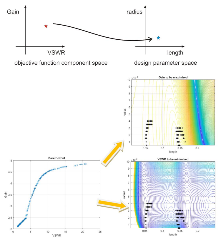
The analysis of the performance of algorithms that we used for single objective optimization showed very good performance of EStra algorithm. For this reason, we decided to test P-EStra algorithm in its bi-objective version. The results of P-EStra optimization are presented in Figure 7, which shows the points located on Pareto-front in objective function space and in design space, respectively.

In turn.

Table 3. Analysis of Pareto EStra Algorithm sensitivity against p and q parameters.

nr	p	q	VSWRmin	Gmax	RG(VSWRmin)	RG(Gmax)	Callmax	Call avg
1	0.1	0.7	1.414632	4.591953	1.996183906	−0.75110921	50	32.97777778
2	0.1	0.75	1.34811575	4.42096375	2.015335957	−0.182593774	67	38.15555556
3	0.1	0.8	1.445974	4.77681375	1.981397027	−2.279198103	73	44.55555556
4	0.1	0.85	1.34811575	4.58963775	2.015335957	−0.678137816	73	56.55555556
5	0.1	0.9	1.39427975	4.771963	2.000326514	−2.080904046	96	78.22222222
6	0.1	0.95	1.48944775	4.5113045	1.965376331	−0.481571138	150	146.4
7	0.15	0.7	1.392596	4.44949325	1.963651401	−0.162833517	60	32.57777778
8	0.15	0.75	1.38949375	4.66783225	1.983534412	−1.249282283	61	38.73333333
9	0.15	0.8	1.34811575	4.47306625	2.015335957	−0.230794849	69	43.75555556
10	0.15	0.85	1.32351925	4.77637975	2.021862788	−2.182204644	73	55.97777778
11	0.15	0.9	1.39020125	4.66783225	1.997481276	−1.249282283	96	78.75555556
12	0.15	0.95	1.32351925	4.44949325	2.021862788	−0.162833517	150	146.1555556
13	0.2	0.7	1.5989625	4.66783225	1.909027684	−1.249282283	44	30.44444444
14	0.2	0.75	1.48614675	4.54797475	1.94579842	−0.708278582	55	35.75555556
15	0.2	0.8	1.33607375	4.499961	2.01051999	−0.362681899	55	41.75555556
16	0.2	0.85	1.32351925	4.771963	2.021862788	−2.080904046	71	53.93333333
17	0.2	0.9	1.33607375	4.5113045	2.01051999	−0.481571138	82	76.17777778
18	0.2	0.95	1.33607375	4.66783225	2.01051999	−1.249282283	150	145.2444444
19	0.25	0.7	1.39020125	4.77561775	1.997481276	−2.367162409	34	30.08888889
20	0.25	0.75	1.32351925	4.5113045	2.021862788	−0.481571138	59	36.15555556
21	0.25	0.8	1.32351925	4.581255	2.021862788	−0.604848098	55	41.31111111
22	0.25	0.85	1.39020125	4.42096375	1.997481276	−0.182593774	69	53.93333333
23	0.25	0.9	1.39020125	4.75530625	1.997481276	−1.979800714	90	76.8
24	0.25	0.95	1.32351925	4.581255	2.021862788	−0.604848098	150	145.2
25	0.3	0.7	1.59242375	4.522489	1.883580045	−0.366358967	34	30.08888889
26	0.3	0.75	1.32351925	4.5070495	2.021862788	−0.42351266	39	35.08888889
27	0.3	0.8	1.38949375	4.5070495	1.983534412	−0.42351266	41	41
28	0.3	0.85	1.32351925	4.47306625	2.021862788	−0.230794849	53	53
29	0.3	0.9	1.5184325	4.66783225	1.955894016	−1.249282283	76	76
30	0.3	0.95	1.5272455	4.547011	1.937485067	−0.44992074	145	145

shows the results of the analysis of P-EStra Algorythm sensitivity to p and q parameters. For each combination of p and q parameters, optimization was performed for 108 starting points. The table presents VSWR_min and G_max that are the best values of those parameters identified over 108 runs. For VSWR_min and the corresponding to this value of antenna gain: G ≠ G_max we have calculated:

$$RG=G-10\ast {\log }_{10}\left(1-{\left(\frac{VSWR-1}{VSWR+1}\right)}^2\right)$$

(2)

Realized gain was used here as a measure of antenna performance that addresses both impedance matching and antenna gain. The RG(VSWR_min) was calculated for the solution which exhibits minimum value of VSWR, while RG(G_max) was for solution with maximal Gain. It can be noted that the selection of p_ann and q_ann parameter influences computational cost of the algorithm, as well as the quality of the final solution.

After examining Table 3, one can note that the average number of objective function calls is moderate and never exceeds the value of 150. For the sake of a comparison, let the typical cost of a GA fur multi-objective optimization be considered: we could reasonably state that a few tenths of individuals (e.g., 30) are mandatory for obtaining a satisfactory approximation of the Pareto front in the case of two objective functions; moreover, several generations (e.g., 10) are necessary for obtaining a good convergence. This means that using a GA, the average number of calls would be in the order of 600 for the same benchmark problem. Furthermore, we were interested to find out a single non-dominated solution rather than an approximating the whole front. This two-fold rationale, i.e., cost-effectiveness and single Pareto-optimal solution was the rationale behind the choice of P-EStra as the optimization algorithm.

2.5. Case Study: Wearable Antenna Design

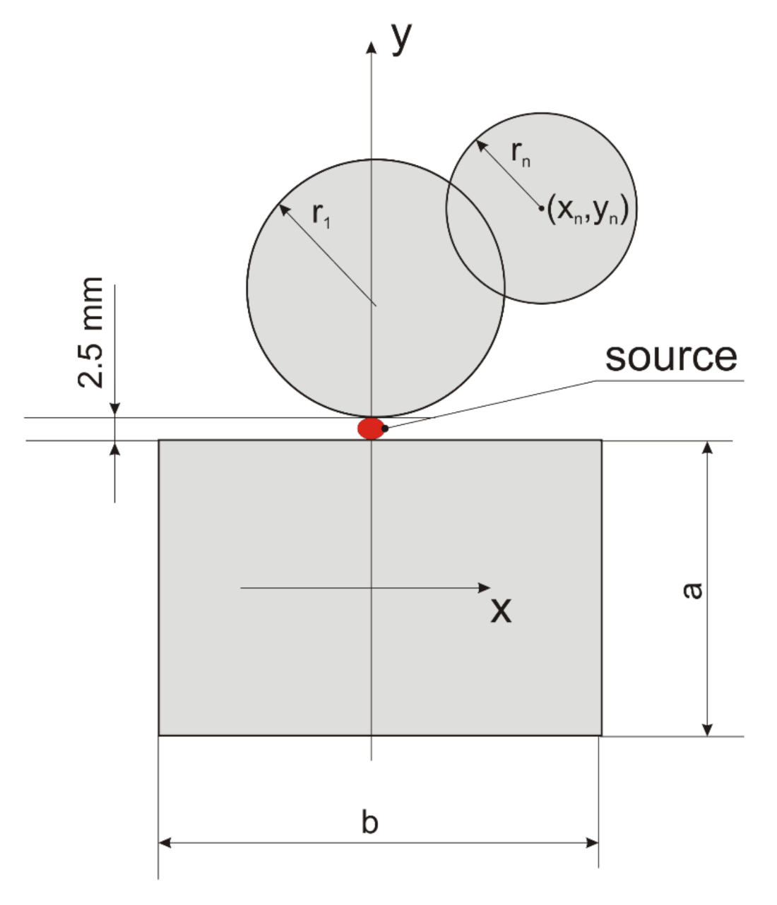
The wearable antenna that we designed is presented in Figure 8. It is a modified UWB antenna that uses a circular monopole. The original antenna was a coplanar waveguide (CPW) fed circular disc monopole antenna [17]. As was shown in [18], antennas that are characterized by a big circle overlapped with four small circles exhibit improved wideband performance over original, single circle antenna. This inspired us to experiment with a circular UWB antenna that has more than one circular element. In our case the design variables are the dimensions of ground plane (a.b), the radius of first circle (r₁) and the relevant coordinates (x_n.y_n), as well as the radius (r_n) of other circles. Figure 8 presents an antenna with two circles (n = 2), but we have also investigated the design with 3 circles.

For circular monopole antenna, the size of the feeding gap has a major influence on the antenna bandwidth. We have found that, having coaxial probe, we could not fabricate the transition of the line to the structure for the gap size that was smaller than 2.5 mm (that is approximately the diameter of the outer conductor of the cable). For this reason, the feeding gap is fixed to 2.5 mm.

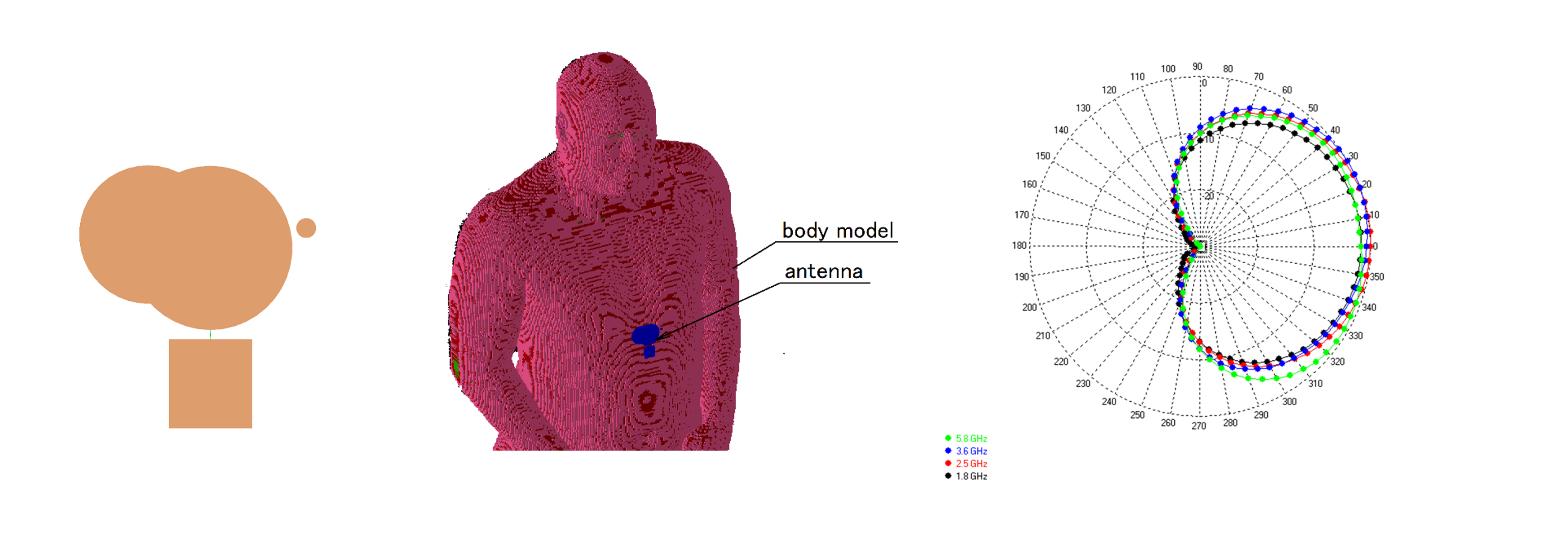
Since we design wearable antenna, human body had to be included in the design stage. To improve the computational cost of wearable antenna optimization process we have used the simplified model of human body presented in [19]. The antenna together with body model is shown in Figure 9. The human body model consists of 2 concentric cylinders. The parameters of models are the following: H = 300 mm, r_o = 271 mm, r_i = 102 mm, ε_o = 3.35, σ_o = 0.36, ε_i = 42.94, σ_i = 2.03. The antenna was placed at half of the model height.

As for the dipole benchmark, we used Remcom XFdtd software to simulate antenna impedance matching and antenna gain G(θ.ϕ = 0°) in z-x plane. The FDTD voxel size was set up to 1 mm for the whole domain and 0.5 mm for the antenna region, respectively. We were aiming at making final prototype of the optimized antenna with thin, flexible substrate (DuPont Pyralux^®). Its thickness is only 25 μm and the thickness of metallization is 35 μm that is much smaller than the voxel size used for antenna simulation. The dielectric constant of base material given by the manufacturer is ε_r = 3.4 and the dielectric loss tg(δ) = 0.005; however, in our previous research we have found that its effective value that can be used for numerical simulation with voxels that are thicker than the substrate (0.5 mm in our case) is ε_r = 1.7 and the dielectric loss tg(δ) = 0.001. The dielectric properties and the dimensions (75 mm by 75 mm) of substrate materials remained unchanged in the optimization process. For the clarity of drawings, we have omitted the layer of this material in figures that are presenting the antenna.

We used P-EStra optimization algorithm presented above to optimize our four-band wearable antenna; the algorithm was implemented in Matlab. In the optimization procedure, we wanted to improve antenna performance in terms of two objective function components: impedance matching and maximum value of Gain in the x-z plane that, assuming on-body location of the antenna, would be the horizontal plane. Those two components were obtained from numerical simulations with the Remcom XFdtd full-wave simulation code, in which the antenna geometry model was created automatically in each iteration of the optimization loop using new geometry parameter values. In XFdtd, four subsequent simulations with sinusoidal excitation (single frequency) in all the considered bands were run for each optimization step in order to simulate antenna gain and impedance matching. We found it to be faster than using broadband excitation and calculating the radiation pattern with postprocessing from steady-state data. In fact, the latter approach was computationally ineffective, and more computer memory was needed to store electromagnetic field for each time step.

We wanted to improve the impedance matching of the antenna in the four bands, which corresponded to minimizing the largest value of VSWR. The other objective was to maximize antenna gain in the bands. Formally, this optimization problem can be stated as follows:

We define:

• g: design vector (geometric parameters defining the multi-band antenna shape)
• Ω_g: set of admissible values
• B₁: band at 1.8 MHz
• B₂: band at 2.4 GHz
• B₃: band at 3.5 GHz
• B₄: band at 5.8 GHz
• VSWR: voltage standing wave ratio
• G₁: maxim gain in x-z plane for band 1
• G₂: maxim gain in x-z plane for band 2
• G₃: maxim gain in x-z plane for band 3
• G₄: maxim gain in x-z plane for band 4
• G: minimum gain of bands 1–4

Starting from a feasible solution g₀ within Ω_g. the following f₁ objective is to be minimized:

$$f_1\left(g\right)=\underset{f\in {\mathrm{B}}_{1234}}{\sup }\left|VSWR\left(g,x,\mathrm{f}\right)\right|,{ \mathrm{where} \mathrm{B}}_{1234}=\underset{k=1}{\overset{4}{{\displaystyle U}}}{\mathrm{B}}_{\mathrm{k}}, g\in {\mathsf{\Omega }}_{\mathrm{g}}$$

and simultaneously. The following f₂ objective is to be maximized (3):

$$f_2\left(g\right)=\underset{f\in {\mathrm{B}}_{1234}}{\inf }\left|G\left(g,x,\mathrm{f}\right)\right|,{ \mathrm{where} \mathrm{B}}_{1234}=\underset{k=1}{\overset{4}{{\displaystyle U}}}{\mathrm{B}}_{\mathrm{k}}, g\in {\mathsf{\Omega }}_{\mathrm{g}}$$

(3)

The P-EStra algorithm makes the doublet (f₁.f₂) evolve from the guess solution g₀ to convergence, treating f₁ and f₂ as individual objectives in mutual conflict.

3. Results of Wearable Antenna Optimization

3.1. Wearable Antenna Optimization

The wearable antenna was optimized with Pareto–Estra algorithm that was tuned basing on the dipole benchmark problem. For this purpose, we set parameters values to p = 0.25 and q = 0.7 because this specific combination allowed to obtain very good impedance matching and antenna gain for a small number of objective function calls, which was equal to 34 (according to line 19 in Table 3).

We started our numerical experiment with optimization of the antenna that has one circle only; this is the classical design of UWB circular monopole antenna. There were 3 design parameters: a, b and r₁. The ground rectangle can be integrated with a printed circuit board that contains electronic circuits. The dimensions of the ground plane (a, b parameters) were limited to 5 cm because we wanted to keep the antenna as small as possible, which is crucial for a wearable application. The maximum radius of the circle allowed in optimization procedure was equal to 25 mm.

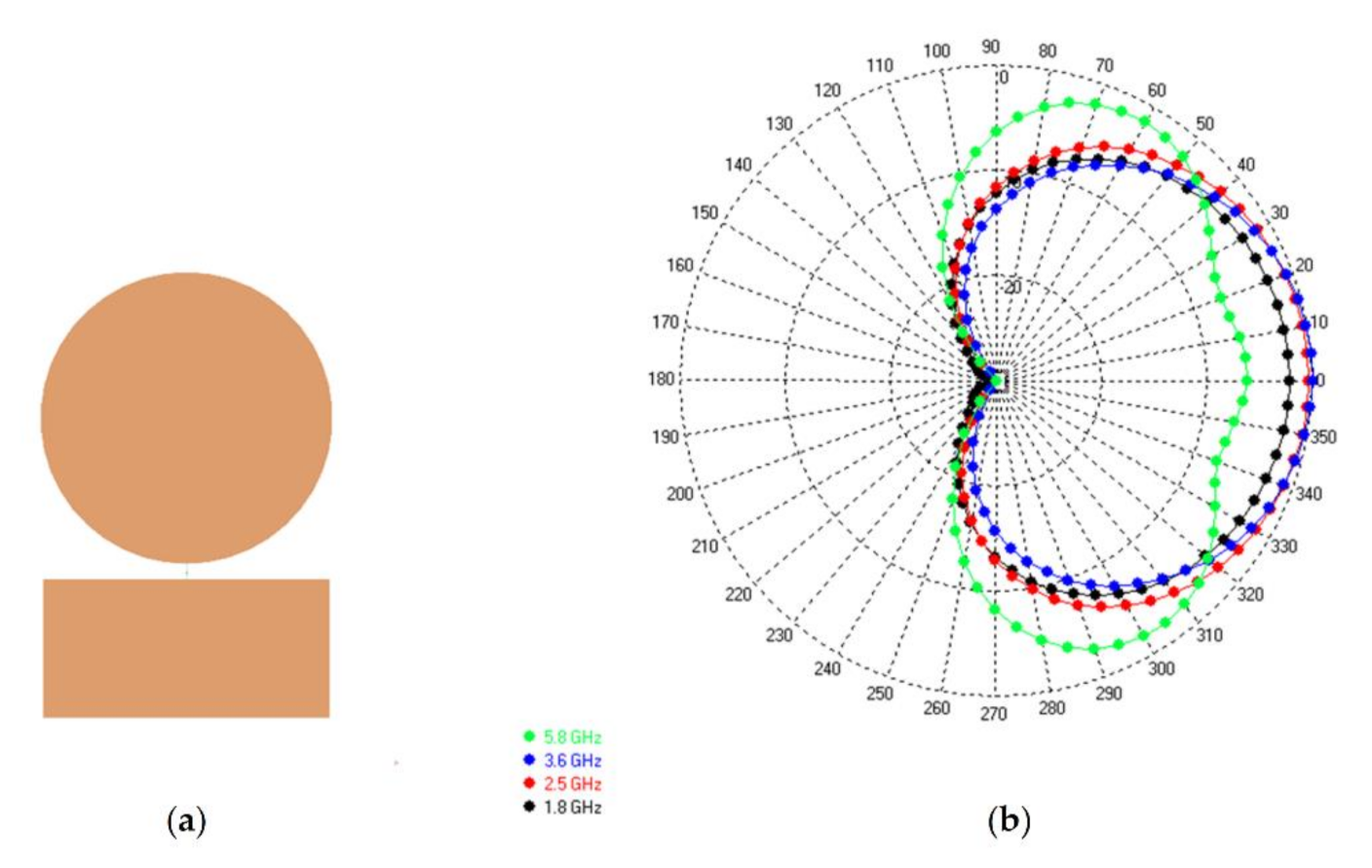
The initial set of design parameter values was selected by trial and error. This provided the starting point for antenna optimization using the P-EStra algorithm. The initial values of design parameters were the following: r_1start = 0.0228, a_start = 0.033, b_start = 0.033. For this starting point the VSWR component of the objective function was VSWR_start = 3.64 and the Gain component was G_start = 0.28 dBi. The constraints in the optimization process were geometry oriented, allowing only for sets of design variable values that preserved the assumed geometry of the antenna without self-intersections or overlapping sections. The optimization process required 56 iterations to satisfy the automatic stopping condition. The condition relies on the ratios of the standard deviation within the current iteration $d_k$ to the initial standard deviation iteration d_0k for each k-th optimization variable. The deviation is normalized across all the variables. The process stops when $\underset{k}{sup}\left[\frac{d_k}{d_{0k}}\right]<s$. where s << 1 is a prescribed search tolerance. This corresponds to the situation when the current search region is sufficiently small for all variables. In this study, basing on experience gathered on optimization of benchmark problem, we assumed $s={10}^{-2}$. Final set of parameters was identified with 56 iterations r_1stop = 0.02366. a_stop = 0.02241. b_stop = 0.04619 and the final objective function components were the following: G_stop = 2.08. VSWR_stop = 2.36. The final geometry of antenna and its radiation pattern is presented in Figure 10.

Table 4. Parameters of optimized single circle antenna.

nr	f [GHz]	G [dBi]	VSWR	RG [dBi]
1	1.8	2.08	1.49	1.91
2	2.5	3.7	1.59	3.47
3	3.6	4.1	1.65	3.83
4	5.8	2.66	2.36	1.96

presents the parameters of optimized antenna: VSWR, gain G and realized gain (RG) for all 4 bands.

The optimization of single circle antenna improved it performance, but its impedance matching is still insufficient. To find the geometry that would have better performance we optimized antenna that consisted of 2 circles. Initial values of design parameters r_1start. a_start and b_start were the same as final parameter*rs of single circle antenna. The set of initial parameters had the following values: r_1start = 0.02366. r_2start = 0.02. x_2start = 0.025 y_2start = 0. a_start = 0.02241. b_start = 0.04619 For this starting point the VSWR component of the objective function was VSWR_start = 2.26 and the Gain component was G_start = 1.33 dBi.

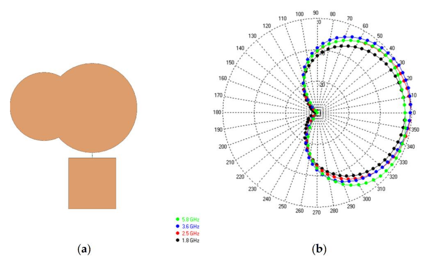
The final set of parameters of two circle antenna was identified with 54 iterations. The final values of design parameters are the following: r_1stop = 0.0209. r_2stop = 0.016. x_2stop = 0.0216. y_2stop = 0.0225. a_stop = 0.02388. b_stop = 0.02217. The final values of objective function components were and G_stop = 1.98. VSWR_stop = 2.26. The final geometry of antenna and its radiation pattern is presented in Figure 11.

Table 5. Parameters of optimized two-circle antenna.

nr	f [GHz]	G [dBi]	VSWR	RG [dBi]
1	1.8	1.98	1.42	1.85
2	2.5	3.74	2.09	3.16
3	3.6	4.13	1.99	3.62
4	5.8	3.08	2.26	2.37

presents the parameters of optimized antenna: VSWR. gain G and realized gain (RG) for all 4 bands.

The double circle antenna exhibits a performance slightly better than the one of the single circle antennae. In this case, VSWR was reduced from 2.36 to 2.26. The gain was similar in both cases: 2.08 dBi for single circle and 1.98 dBi for two circles and is comparable to half-wave dipole antenna.

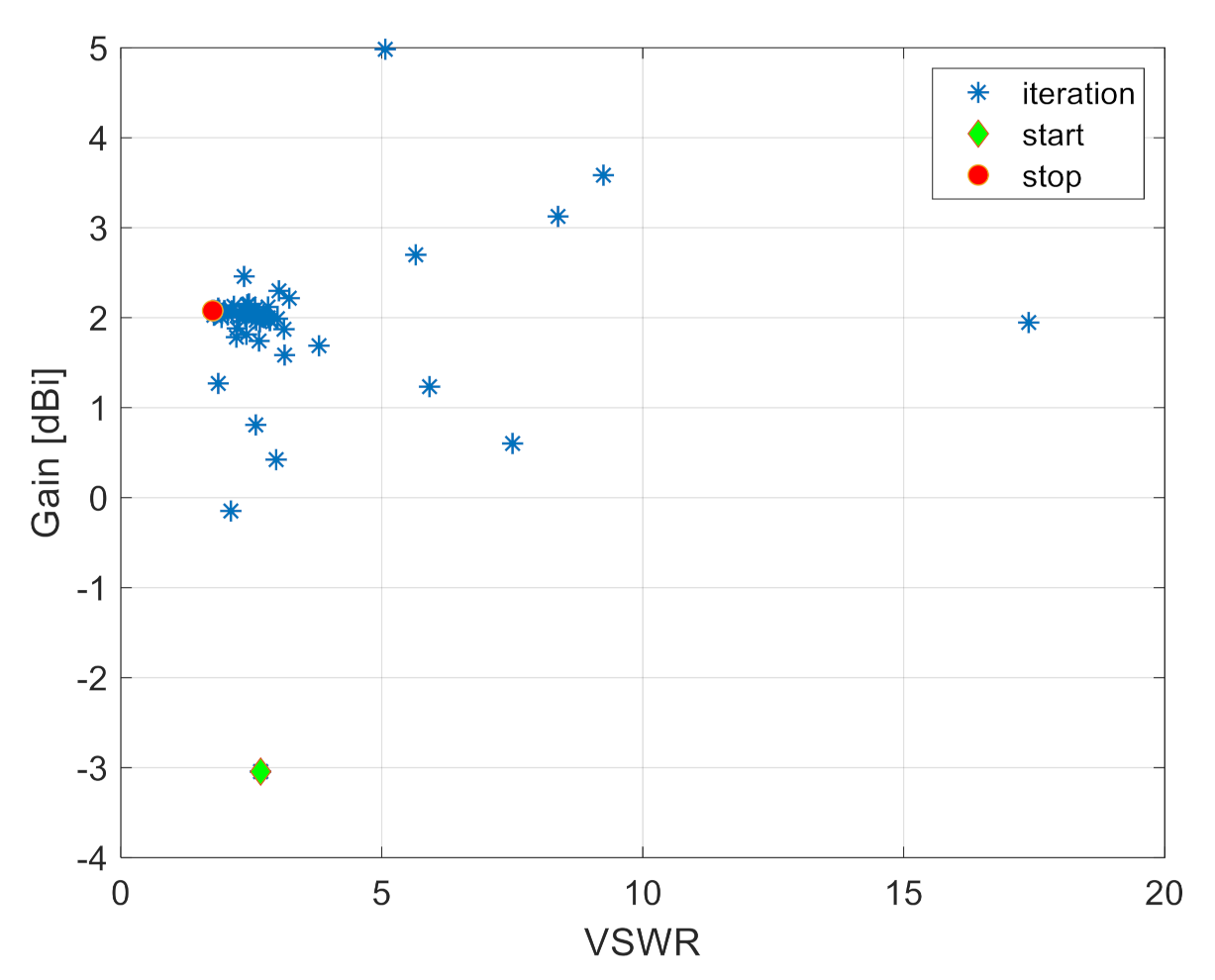
Since we design wearable antenna, we wanted to obtain better impedance matching because the presence of clothes can detune the antenna. Having better impedance matching, there would be some tolerance to this effect even for antenna covered with other materials. For this reason, we have investigated a more complex antenna geometry, that consists of 3 circles. Adding another circle brings 3 more design variables, which in turn increases the number of iterations and overall computational cost of optimization procedure. In our opinion, 3 circle antennae that are controlled by 9 design variables implies a feasible number of parameters to handle by P-EStra algorithm. Initial values of design parameters were inspired by the geometry of optimized two circle antenna and had following values: r_1start = 0.0209, r_2start = 0.016, x_2start = 0.0216, y_2start = 0.0225, r_3start = 0.00279, x_3start = 0.02793, y_3start = −0.01242, a_start = 0.02388, b_start = 0.02217. For this starting point, the VSWR component of the objective function was VSWR_start = 2.21 and the Gain component was G_start = 2.0 dBi.

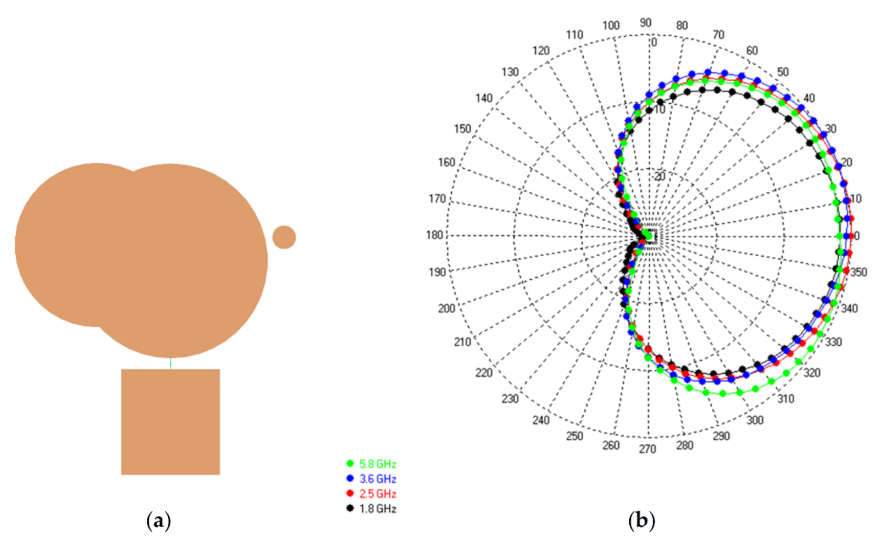
The history of the optimization process from the initial point in the objective function space is shown in Figure 12. The final set of parameters of two circle antenna was identified after 87 iterations. The final values of design parameters are the following: r_1stop = 0.02195, r_2stop = 0.01852, x_2stop = 0.02552, y_2stop = 0.01648, r_3stop = 0.00266, x_3stop = 0.02725, y_3stop = −0.02574, a_stop = 0.02384, b_stop = 0.0226. The final values of objective function components were G_stop = 2.08, VSWR_stop = 1.76. The final geometry of the antenna and its radiation pattern is shown in Figure 13.

Table 6. Parameters of optimized three circle antenna.

nr	f [GHz]	G [dBi]	VSWR	RG [dBi]
1	1.8	2.08	1.18	2.05
2	2.5	3.75	1.76	3.41
3	3.6	3.73	1.69	3.43
4	5.8	3.04	1.73	2.72

presents the parameters of optimized antenna: VSWR, gain G and realized gain (RG) for all four bands.

The antenna with 3 circles has the best impedance matching compared to single circle antenna and two circle antennae. The maximum value of VSWR is 1.76. At the same time the minimum value of Gain is 2.08. The smallest value of realized gain was for 1.8 GHz and was equal to 2.05 dBi. Current distribution for antenna with 3 circles is presented in

Table 7. Parameters of optimized three circle antenna.

nr	f [GHz]	Current Distribution on the Antenna Surface
1	1.8
2	2.5
3	3.6
4	5.8

for all 4 considered frequencies.

Wearable antenna was optimized with simplified model of human body that represents only its part with cylindrical structure. To verify the radiation pattern of three circle antenna in more realistic scenario, we have used heterogenous model of entire body that is available in Remcom Xfdtd program. It has 3mm voxel size and models not only the shape of human body, but also the inner tissues. We assumed that the antenna is located in the front of the torso, at the distance of 10 mm from the surface of the model. Figure 14 presents the position of antenna on heterogenous model and obtained radiation pattern in horizontal plane. The results are very similar to those obtained with simplified model. The maximum gain varies in this case form 2.5 dBi for 1.8 GHz to 4.5 dBi for 2.5 GHz.

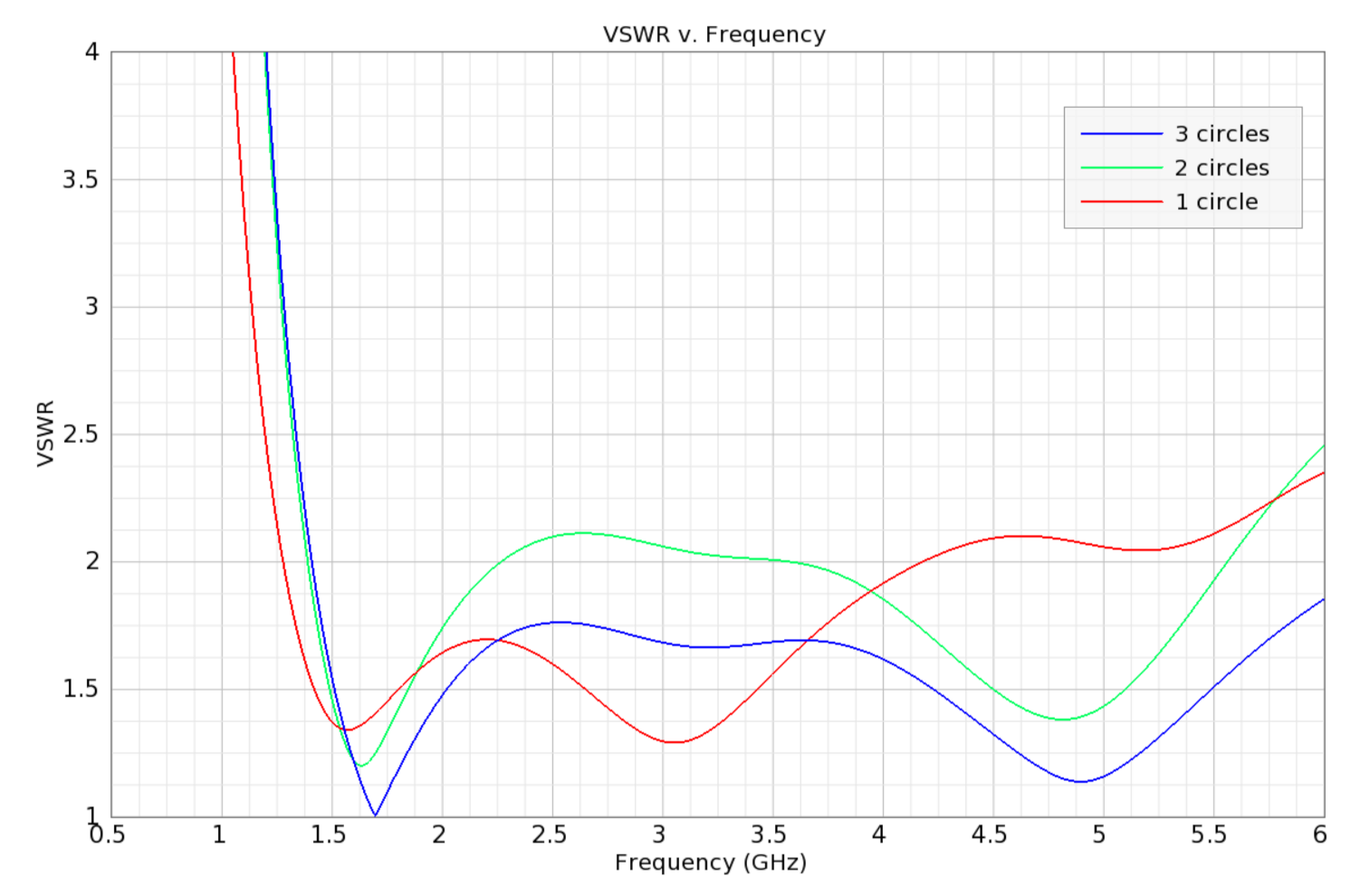
In Figure 15 the impedance matching of three optimized antennas is presented for on-body position. It is evident that optimized 3 circle antennae have the best impedance matching for all considered bands from 1.8 GHz to 5.8 GHz.

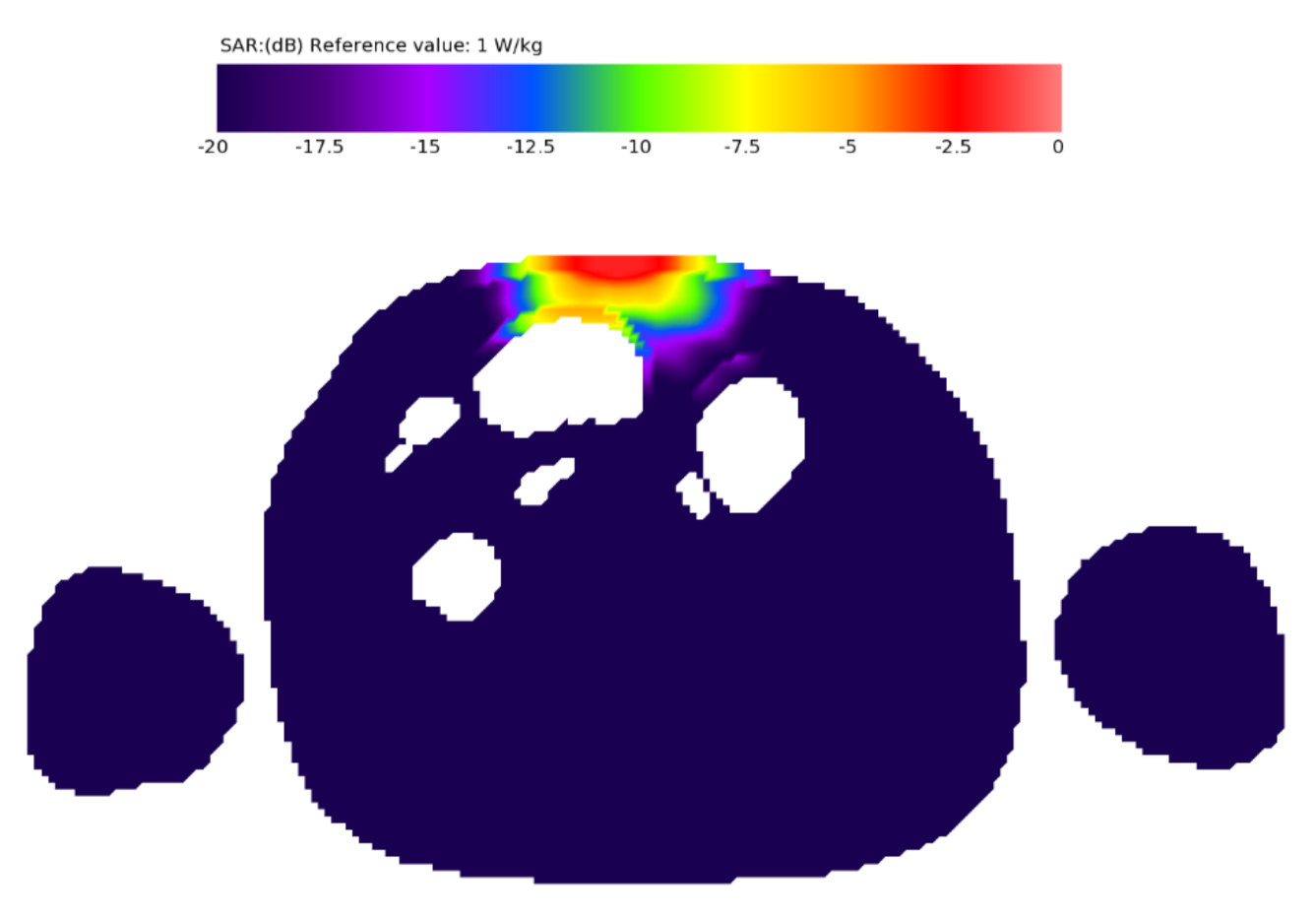
Wearable antenna is the source of electromagnetic wave that is partially absorbed by the human body. This effect can be illustrated with Specific Absorption Rate (SAR) parameter that presents the amount of energy dissipated by the mass of human tissues. For the optimized antenna with three circular elements, we have simulated the SAR parameter using heterogenous model of human body that is available in Remcom Xfdtd software. The possible application of this antenna could be the portable, battery operated device with limited power resources. Thus, for SAR simulations we have assumed that the power of transmitter connected to the antenna is 200 mW, which corresponds to the power class 2 of LTE and 5 G portable terminals. The distribution of the SAR parameter on the cross-section of the body is presented in Figure 16. It shows that the body region that is close to the antenna absorbs the most of energy. The maximum values of SAR (SAR_max) and average values for the whole body (SAR_AVG) averaged for 10 g of tissue are presented in

Table 8. SAR values averaged in 10 g of tissue.

nr	f [GHz]	SARmax [W/kg]	SARAVG [W/kg]
1	1.8	0.894	0.00094
2	2.5	0.335	0.00045
3	3.6	0.688	0.00041
4	5.8	0.032	0.00002

for all considered bands. The SAR values are below the limits for mobile phones that for Europe are 2 W/kg.

3.2. Assessment of Antenna Prototype

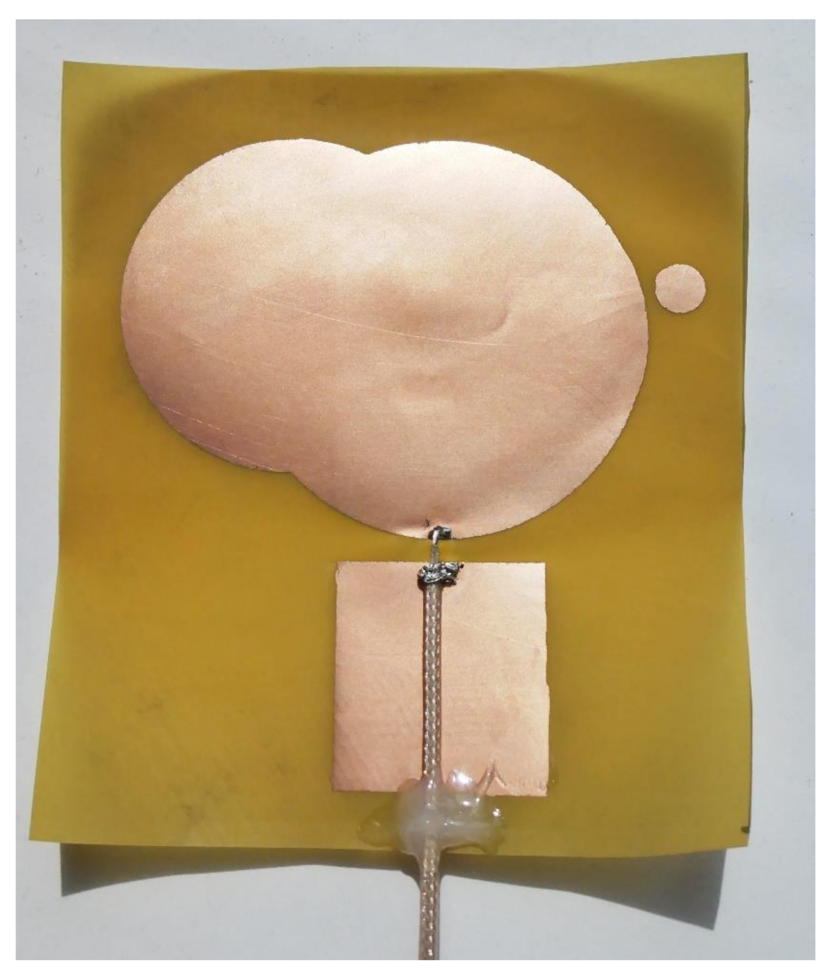
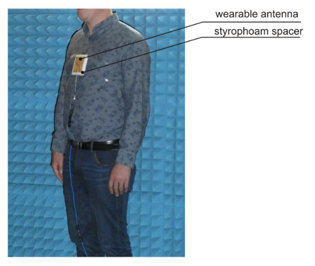
The impedance matching of the optimized antenna was experimentally assessed using a prototype. We used DuPont Pyralux^® material that is a polymer foil with one side of coper metallization. The thickness of the base material is only 25 μm and the thickness of metallization is 35 μm. This makes the antenna flexible and lightweight what is beneficial in wearable applications. The dielectric constant of base material given by the manufacturer is ε_r = 3.4 and the dielectric loss tg(δ) = 0.005; however, in our previous research we have found that its effective value that can be used for numerical simulation with voxels that are thicker than the substrate (0.1 mm in our case) is ε_r = 1.7 and the dielectric loss tg(δ) = 0.001 [20] Due to the small thickness of substrate and its flexibility we used laser printer to put the mask on the substrate. To make it solid, we printed 4 layers of mask and then etched the metallization. The prototype is presented in Figure 17. The impedance matching of the prototype antenna located on human subject was measured using a Rohde & Schwarz ZVB 14 vector network analyzer. To avoid reflections that may influence the results of measurements they were conducted in anechoic chamber. The antenna was attached to the torso of human subject. To control the distance between antenna and human body we have used the Styrofoam spacer that is presented in Figure 18. The prototype antenna was fed by a coaxial probe and the calibration plane was moved to the end of the coaxial cable.

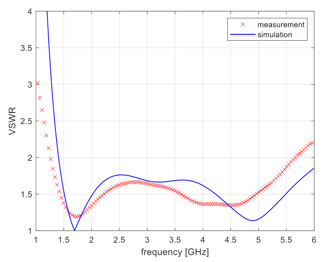
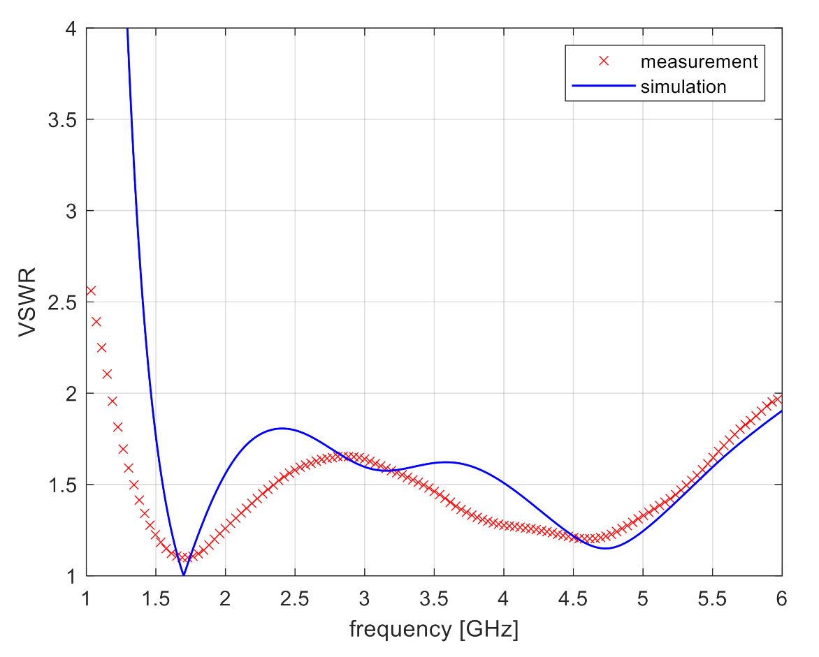
The impedance matching of the prototype for antenna located 10 mm, 20 mm and 30 mm from body are presented in Figure 19, Figure 20, Figure 21. The results of measurements are compared with results of simulations obtained with NMR human body model. The results of measurements are similar to the results of simulations. The impedance matching of the prototype antenna is satisfactory in all assumed bands, with VSWR < 2.2. For the antenna located 10 mm from body, the VSWR value for 5.8 GHz is 2.2, which may result from a difference between a numerical model of the body and a human subject.

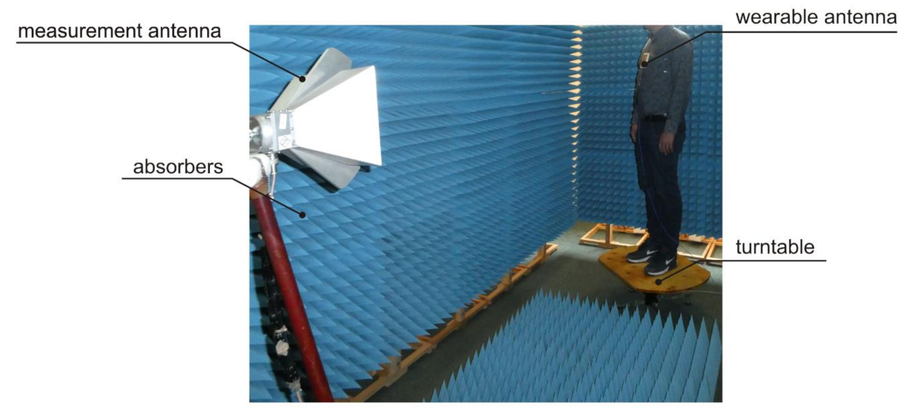
The radiation pattern of the prototype antenna was measured in anechoic setup presented in Figure 22. The measurement antenna was a Rohde & Schwarz HF 907. It was connected to a Rohde & Schwarz SMB 100A signal generator. The prototype antenna was attached to human subject that was standing on the turntable. For each angle of rotation (with 5 degrees step), the power of signal was measured with Rohde & Schwarz FSC 6 spectrum analyzer. The antenna gain was measured using gain comparison method [21]. After the experiment, the human subject and prototype antenna were replaced with second Rohde & Schwarz HF 907 that we used as standard gain antenna, for which the received power was measured. Knowing the gain of HF 907 antenna, we then recalculated received power level into antenna gain. The results of radiation pattern and antenna gain measurements are presented in

Table 9. Results of radiation pattern and antenna gain measurements in horizontal plane.

Frequency [GHz]	Simulated Gain [dBi]	Measured Gain [dBi]	Radiation Pattern
1.8	2.5	2
2.5	6	5
3.6	2.6	1.8
5.8	5.9	4

.

Results of radiation pattern measurements correspond with results of simulations. Some difference may result with antenna placement on the body that could be slightly different in the case of simulations and measurements. The antenna gain obtained from measurements was slightly lower than obtained from simulations. This could be caused by losses introduced by feeding cable.

4. Discussion

The benchmark problem proposed in this paper allowed us to study the performance of different optimization algorithms. We used this to compare properties of single-objective optimization routines, as well as for analysis of bi-objective optimization strategy. Due to its effective numerical implementation that is based on pre-calculated lookup table implemented in Matlab it was possible to perform an experiment with wide range of 108 starting points for each algorithm run. Even for this rich set of optimization runs, it took only few minutes on typical personal computer to obtain results. This feature of the proposed benchmark allowed us deep study of bi-objective EStra algorithm sensitivity to its parameters. We examined 30 combinations of algorithm parameters and each combination was launched from 108 starting points. This experiment was completed in the time of 1 h.

The proposed antenna design based on ultra-wideband circular monopole supplemented with two additional circular elements showed good performance in a wide range of frequencies. The impedance matching of this antenna in the proximity of human body is characterized by VSWR < 1.76 for the frequency range from 1.8 GHz to 5.8 GHz. Also, the antenna gain is comparable to half wave dipole and is not smaller than 2.08 dBi for 1.8 GHz, while for other bands it was greater than 3 dBi. Such parameters of wearable antenna are satisfactory considering its small dimensions. The largest dimension (in y direction referring to Figure 7) is equal to 70.4 mm. This antenna is compact and suitable for wearable applications. The important feature of this antenna is that it can be manufactured with thin, flexible substrate: thanks to this, it remains flexible and can be integrated with clothes.

Future research will focus on improving the technology of prototype fabrication. The laser printing of mask used for antenna etching will be replaced with inkjet printing that allows to keep substrate in fixed position. This will allow for more precise alignment of multiple layers and more precise fabrication of antenna prototype.

We also plan to assess the performance of the antenna with respect to its gain for on-body location including different on-body locations (e.g., torso, arm, leg). The results obtained in this paper address only the case of antenna located on torso because the body model applied here was elaborated for this part of the body.

5. Conclusions

In this paper we present a simple benchmark problem that is suitable for analysis of optimization algorithm performance that is applied to antenna design. It was successfully used for identifying the values of algorithm parameters that we applied for design optimization.

The proposed design of a wearable antenna was significantly improved by an optimization algorithm that was based on evolution strategy. The final project is characterized by good impedance matching and acceptable gain for a wide range of frequencies (from 1.8 GHz to 5.8 GHz). This antenna was optimized being located in the proximity of the human body model and can operate well in proximity of the human body.

In our opinion this design can be applicable to wearable systems for wireless patient monitoring.

References

- El-Rashidy, N.; El-Sappagh, S.; Islam, S.M.R.; El-Bakry, H.M.; Abdelrazek, S. Mobile Health in Remote Patient Monitoring for Chronic Diseases: Principles, Trends, and Challenges. Diagnostics 2021, 11, 607. [Google Scholar] [CrossRef] [PubMed]
- Olatinwo, D.D.; Abu-Mahfouz, A.; Hancke, G. A Survey on LPWAN Technologies in WBAN for Remote Health-Care Monitoring. Sensors 2019, 19, 5268. [Google Scholar] [CrossRef] [PubMed] [Green Version]
- Rozas, A.; Araujo, A.; Rabaey, J.M. Analyzing the Performance of WBAN Links during Physical Activity Using Real Multi-Band Sensor Nodes. Appl. Sci. 2021, 11, 2920. [Google Scholar] [CrossRef]
- Youssef, S.B.H.; Rekhis, S.; Boudriga, N. Design and Analysis of a WBAN-Based System for Firefighters. In Proceedings of the 2015 International Wireless Communications and Mobile Computing Conference (IWCMC), Dubrovnik, Croatia, 24–28 August 2015; pp. 526–531. [Google Scholar]
- García-Martín, J.P.; Torralba, A. Model of a Device-Level Combined Wireless Network Based on NB-IoT and IEEE 802.15.4 Standards for Low-Power Applications in a Diverse IoT Framework. Sensors 2021, 21, 3718. [Google Scholar] [CrossRef] [PubMed]
- Balanis, C.A. Antenna Theory, Analysis and Design; John Wiley & Sons: Hoboken, NJ, USA, 2016. [Google Scholar]
- Luebbers, R. XFDTD and Beyond-from Classroom to Corporation. In Proceedings of the 2006 IEEE Antennas and Propagation Society International Symposium, Albuquerque, NM, USA, 9–14 July 2006; pp. 119–122. [Google Scholar]
- Homsup, N.; Breakall, J. Application of XFDTD and FEKO Program to the Analysis of Planar Antennas. In Proceedings of the 2010 10th International Symposium on Communications and Information Technologies, Tokyo, Japan, 26–29 October 2010; pp. 646–650. [Google Scholar]
- Nelder, J.A.; Mead, R. A simplex method for function minimization. Comput. J. 1965, 7, 308–313. [Google Scholar] [CrossRef]
- Matlab documentation: Fminsearch. Available online: https://www.mathworks.com/help/matlab/ref/fminsearch.html (accessed on 20 April 2021).
- Byrd, R.H.; Hribar, M.E.; Nocedal, J. An Interior Point Algorithm for Large-Scale Nonlinear Programming. SIAM J. Optim. 1999, 9, 877–900. [Google Scholar] [CrossRef]
- Byrd, R.H.; Gilbert, J.C.; Nocedal, J. A Trust Region Method Based on Interior Point Techniques for Nonlinear Programming. Math. Program. 2000, 89, 149–185. [Google Scholar] [CrossRef] [Green Version]
- Matlab documentation: Fmincon. Available online: https://www.mathworks.com/help/optim/ug/fmincon.html (accessed on 20 April 2021).
- Shanno, D.F. Conditioning of Quasi-Newton Methods for Function Minimization. Math. Comput. 1970, 24, 647–656. [Google Scholar] [CrossRef]
- Matlab documentation: Fminunc. Available online: https://www.mathworks.com/help/optim/ug/fminunc.html (accessed on 20 April 2021).
- Di Barba, P. Multiobjective Shape Design in Electricity and Magnetism; Springer: Berlin/Heidelberg, Germany, 2010. [Google Scholar]
- Liang, J.; Guo, L.; Chiau, C.C.; Chen, X. CPW-fed circular disc monopole antenna for UWB applications. In Proceedings of the IWAT 2005. IEEE International Workshop on Antenna Technology: Small Antennas and Novel Metamaterials, Singapore, 7–9 March 2005; pp. 505–508. [Google Scholar]
- Taha-Ahmed, B.; Lasa, E.M.; Sanchez Olivares, P.; Masa-Campos, J.L. Uwb antennas with multiple notched-band function. PIER Lett. 2018, 77, 41–49. [Google Scholar] [CrossRef] [Green Version]
- Januszkiewicz, Ƚ.; Barba, P.D.; Hausman, S. Automated Identification of Human-Body Model Parameters. Int. J. Appl. Electromagn. Mech. 2016, 51, S41–S47. [Google Scholar] [CrossRef]
- Januszkiewicz, Ł.; Barba, P.; Hausman, S. Optimization of wearable microwave antenna with simplified electromagnetic model of the human body. Open Phys. 2017, 15, 1055–1060. [Google Scholar] [CrossRef] [Green Version]
- Stutzman, W.L.; Thiele, G.A. Antenna Theory and Design, 3rd ed.; Wiley: Hoboken, NJ, USA, 2012. [Google Scholar]
Figure 1.
Dipole antenna geometry.
Figure 2.
Gain of dipole in the plane parallel to the antenna G(θ)—for different antenna length.
Figure 3.
Impedance matching of dipole antenna for different antenna length.
Figure 4.
Design parameter space (L.r) and objective function component space (VSWR. G) for dipole benchmark.
Figure 5.
Set of 108 starting points regularly located in the parameter space (L.r) that are marked with “*” and objective function component—VSWR presented with contour lines for dipole benchmark.
Figure 6.
Flow-chart of P-EStra algorithm.
Figure 7.
Results of P–EStra optimization located on Pareto–front in objective space and in design space.
Figure 8.
Design of wearable multiband antenna: design variables.
Figure 9.
Simplified human body model used for antenna optimization.
Figure 10.
Single circle antenna optimized with Pareto Estra algorithm: (a)—antenna geometry. (b)—radiation pattern in x-z plane for on-body position.
Figure 11.
Two circle antennae optimized with Pareto Estra algorithm: (a)—antenna geometry. (b)—radiation pattern in x-z plane for on-body position.
Figure 12.
Objective space: history of optimization process of antenna with 3 circles.
Figure 13.
Three circle antenna optimized with P-EStra algorithm: (a)—antenna geometry. (b)—radiation pattern in x-z plane for on-body position.
Figure 14.
Three circle optimized antenna radiation pattern: (a)—antenna position on heterogenous model. (b)—radiation pattern in horizontal plane.
Figure 15.
The impedance matching of three optimized antennas for on-body position.
Figure 16.
The distribution of Specific Absorption Rate (SAR) parameter in the cross-section of human body model, at the position of antenna for 3.5 GHz.
Figure 17.
The prototype of three circle antenna fabricated with thin flexible substrate.
Figure 18.
The prototype antenna attached to human subject for measurements.
Figure 19.
The impedance matching of prototype antenna for on-body location for 10 mm distance from the body.
Figure 20.
The impedance matching of prototype antenna for on-body location for 20 mm distance from the body.
Figure 21.
The impedance matching of prototype antenna for on-body location for 30 mm distance from the body.
Figure 22.
The measurement setup for measurement of wearable antenna radiation pattern.