the Creative Commons Attribution 4.0 License.
the Creative Commons Attribution 4.0 License.
 | 13 Sep 2021
Mesospheric gravity wave activity estimated via airglow imagery, multistatic meteor radar, and SABER data taken during the SIMONe–2018 campaign
Jorge L. Chau
Harikrishnan Charuvil Asokan
Michael Gerding
We describe in this study the analysis of small and large horizontal-scale gravity waves from datasets composed of images from multiple mesospheric airglow emissions as well as multistatic specular meteor radar (MSMR) winds collected in early November 2018, during the SIMONe–2018 (Spread-spectrum Interferometric Multi-static meteor radar Observing Network) campaign. These ground-based measurements are supported by temperature and neutral density profiles from TIMED/SABER (Thermosphere, Ionosphere, Mesosphere Energetics and Dynamics/Sounding of the Atmosphere using Broadband Emission Radiometry) satellite in orbits near Kühlungsborn, northern Germany (54.1∘ N, 11.8∘ E). The scientific goals here include the characterization of gravity waves and their interaction with the mean flow in the mesosphere and lower thermosphere and their relationship to dynamical conditions in the lower and upper atmosphere. We have obtained intrinsic parameters of small- and large-scale gravity waves and characterized their impact in the mesosphere via momentum flux (FM) and momentum flux divergence (FD) estimations. We have verified that a small percentage of the detected wave events is responsible for most of FM measured during the campaign from oscillations seen in the airglow brightness and MSMR winds taken over 45 h during four nights of clear-sky observations. From the analysis of small-scale gravity waves (λh < 725 km) seen in airglow images, we have found FM ranging from 0.04–24.74 m2 s−2 (1.62 ± 2.70 m2 s−2 on average). However, small-scale waves with FM > 3 m2 s−2 (11 % of the events) transport 50 % of the total measured FM. Likewise, wave events of FM > 10 m2 s−2 (2 % of the events) transport 20 % of the total. The examination of large-scale waves (λh > 725 km) seen simultaneously in airglow keograms and MSMR winds revealed amplitudes > 35 %, which translates into FM = 21.2–29.6 m2 s−2. In terms of gravity-wave–mean-flow interactions, these large FM waves could cause decelerations of FD = 22–41 m s−1 d−1 (small-scale waves) and FD = 38–43 m s−1 d−1 (large-scale waves) if breaking or dissipating within short distances in the mesosphere and lower thermosphere region.
- Article
(17371 KB) -
Supplement
(5246 KB) - BibTeX
- EndNote


Atmospheric gravity waves represent a class of atmosphere oscillations where buoyancy is the restoring force. These waves transport momentum and energy over large distances within the atmosphere and have as primary sources troposphere disturbances like flow over topography, convective systems, or jets (e.g., Vincent and Alexander, 2020). To preserve kinetic energy, the amplitudes of the gravity waves grow nearly exponentially as they propagate upward into less dense air at higher altitudes. When these waves break and dissipate, they deposit their momentum and energy into the background atmosphere. This affects the atmosphere over a broad range of scales, from local generation of turbulence to forcing of large-scale circulation (Fritts and Alexander, 2003; Vincent and Alexander, 2020).
This dynamical forcing is most prominent within the mesosphere and lower thermosphere (MLT) at altitudes of typically 50–130 km. Within this range, a large fraction of upward-propagating gravity waves reach their maximum amplitudes and break. The resulting dynamical forcing causes a global-scale circulation within the mesosphere with strong upwelling within the summer polar region and downwelling within the winter polar region (Houghton, 1978; Holton, 1984). Adiabatic cooling and heating connected to this circulation cause thermal conditions within the mesosphere to deviate greatly from radiative equilibrium (Solomon et al., 1987; Vargas et al., 2015).
The role of gravity waves is further complicated as they interact with the background flow as they propagate through the atmosphere. This results in an altitude-dependent filtering of the gravity wave spectrum by the background wind, planetary, and tidal waves. The gravity wave spectrum reaching higher altitudes thus carries an imprint of the dynamics at lower altitudes. Interactions between gravity waves and the mean flow and subsequent wave breaking then generate secondary waves within the mesosphere that propagate both upward and downward. This happens through the creation of temporally and spatially localized momentum and energy fluxes, which successively create strong local body forces and flow imbalances which then excite the secondary waves (Fritts et al., 2006; Vargas et al., 2016; Vadas et al., 2018; Vadas and Becker, 2018; Becker and Vadas, 2018).
While today the essential nature of the wave-driven circulation of the middle atmosphere is known, important mechanisms and interactions remain to be quantified. Most notably, this concerns wave sources, wave dissipation, and therefore the resulting forcing of the mean flow. A decisive quantity to be specified is the directional FM, including its altitude dependence and its spectral distribution with reference to horizontal (λh) and vertical (λz) wavelengths. Ern et al. (2011) have provided global distributions of gravity wave FM in the mesosphere for the first time using global temperature measurements by the Sounding of the Atmosphere using Broadband Emission Radiometry (SABER). They have shown clearly the dependency of gravity wave FM deposition according to latitude and longitude (non‐uniform longitudinal distribution of flux) at different altitude levels from the stratosphere up to the mesosphere along with their seasonal and longer‐term variations. Also, attempts of estimating FM of small-scale, short-period waves using multiple observation platforms such as aircraft, lidar, airglow sounders, radars, and satellites have been done (e.g, Suzuki et al., 2010; Bossert et al., 2015), while Gong et al. (2019) and Reichert et al. (2019) have relied on lidar, meteor radar, and SABER data to study large-scale, long-period waves perturbing the mesosphere temperature and the winds simultaneously. These studies report attempts to characterize the wave field and provide FM estimations of observed events as well.
To bridge gaps in gravity wave dynamics while estimating their FM, an observation campaign named SIMONe–2018 (Spread-spectrum Interferometric Multi-static meteor radar Observing Network) was carried from 2–9 November 2018, to collect a large number of specular meteor echoes from several locations (e.g., Vierinen et al., 2019; Charuvil et al., 2020). Also, an all-sky airglow imager system running out of the Leibniz Institute of Atmospheric Physics, Kühlungsborn, Germany, observed the region in parallel to provide image data of the mesosphere and the horizontal structure of atmospheric oscillations during the campaign.
SIMONe–2018 campaign measurements permit us to study distinct spatial and temporal scales of gravity waves perturbing the background wind and the airglow simultaneously. In this paper, we have analyzed all-sky imager (ASI) airglow images and multistatic specular meteor radar (MSMR) wind data to access small-scale as well as large-scale gravity wave dynamics using two different analysis methods for each wave category. Airglow images are processed directly using our auto-detection method for small-scale (< 725 km), short-period (< 1 h) gravity waves aided by MSMR background wind measurements for Doppler correction of wave-apparent periods (τo). For nights presenting obvious large-scale (> 725 km), long-period (> 1 h) oscillations, wave features are studied via direct examination of large-amplitude wind fluctuations and airglow keogram spectral analysis. We have also obtained measurements of the neutral density, temperature, and OH emission volume emission rates from the SABER instrument (Russell et al., 1999; Mlynczak, 1997) aboard the NASA TIMED (Thermosphere, Ionosphere, Mesosphere Energetics and Dynamics) satellite (http://saber.gats-inc.com, last access: 6 September 2021) to determine the state of the mesosphere region near the observatory during the campaign. This study shows remarkable instances of waves perturbing the airglow and the wind, providing a singular opportunity to examine the linear gravity wave theory's predictions and the occurrence of gravity waves perturbing multiple mesospheric quantities simultaneously. The main contributions here regard the fraction of observed waves carrying substantial FM with the potential to impart significant changes in the 75–110 km dynamics since we show evidence that most observed waves likely experience dissipation in that region.
2.1 All-sky airglow imager
An all-sky imager (ASI) assembled at Boston University was deployed in late 2016 at the Leibniz Institute of Atmospheric Physics (IAP) in Kühlungsborn, Germany. The imager is equipped with an Andor back-illuminated bare CCD camera and a 30 mm fish-eye lens which record several nightglow emissions over the entire 180∘ of the night sky. Andor's iKon-M 934 camera is a 1024 × 1024 array and 13 µm pixel pitch with a 13.3 × 13.3 mm active image area. High sensitivity is achieved through a combination of > 90 % QE (quantum efficiency; back-illuminated sensor), low noise readout electronics, and deep TE (thermoelectric) cooling down to −60∘C. The ASI system uses six interference filters enabling the observation of four mesosphere airglow emissions with a background filter for the hydroxyl emission. A filter for the thermospheric redline (at 630.0 nm) is also available, but images of this emission were not taken during SIMONe–2018 due to filter technical issues. The imaging system operates autonomously via a PC on a nightly basis during moonless periods. Images are obtained on a continuously repeating cycle every ∼ 2 min with each particular filter accessed every ∼ 10 min. The specifications of filter wavelengths and integration times are in Table 1. Emission altitudes are discussed in Sect. 2.3. Preprocessed, low-resolution images collected by the ASI are available for visualization at http://sirius.bu.edu/data/ (last access: 6 September 2021). Raw images used in this study are available at https://doi.org/10.13012/B2IDB-8585682_V1 (Vargas, 2021).
Table 1Configuration of the all-sky imager system used to collect airglow images during the SIMONe–2018 campaign. Airglow images of the campaign are available at http://sirius.bu.edu/data/. NaD represents a sodium atom at the D transition line.

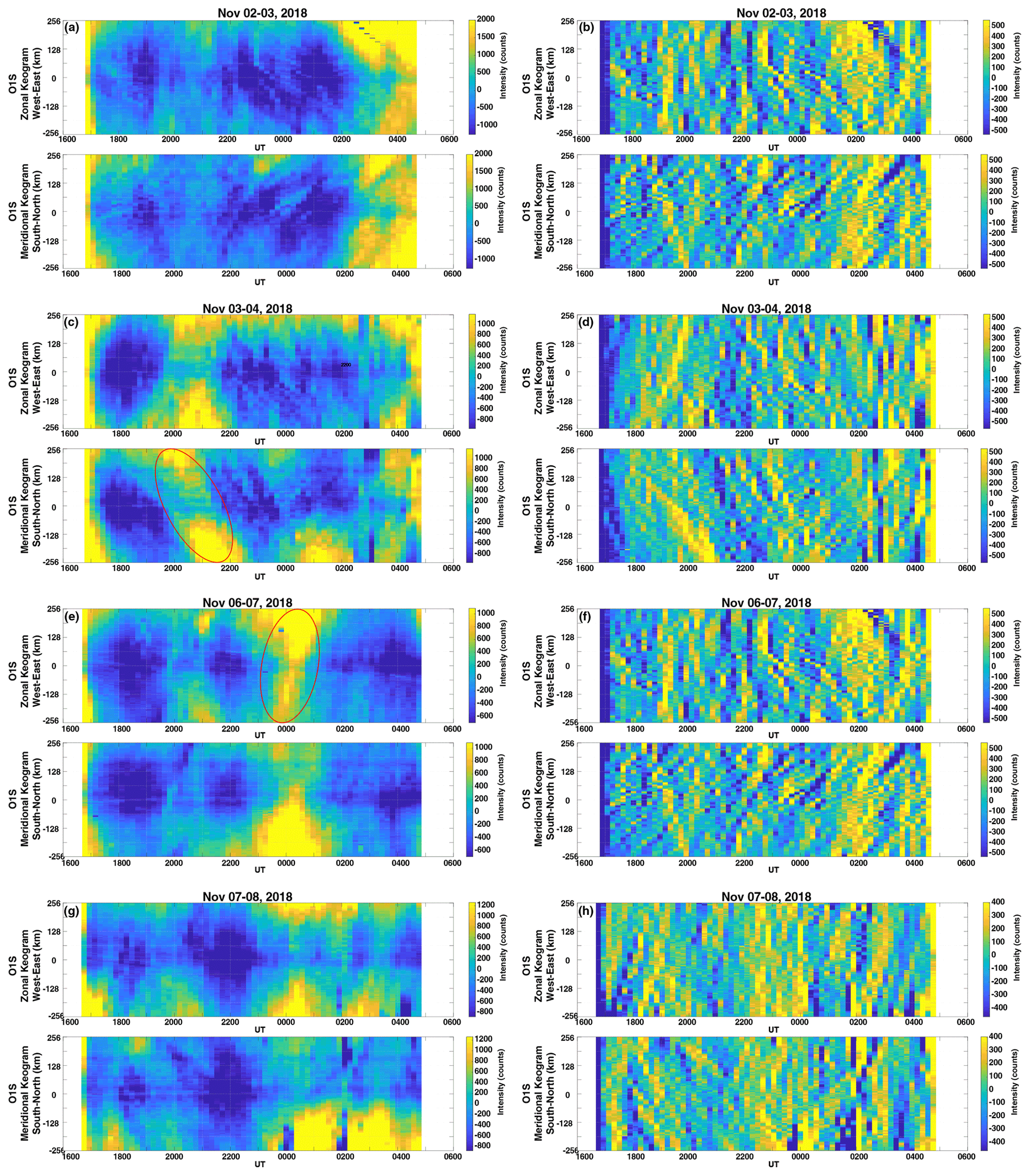
Figure 1Composite keograms of O(1S) airglow images taken on clear nights during the SIMONe–2018 campaign. The keograms in panels (a), (c), (e), and (g) were built using light frame images, while keograms in panels (b), (d), (f), and (h) were built using TD images. Time–difference keograms show short-period waves at higher contrast, while light frame keograms show mainly long-period oscillations. Note the enhanced airglow brightness (red ellipses) on 3–4 November (meridional keogram) and 6–7 November (zonal keogram) associated with large-scale gravity waves also seen in wind fluctuations of Fig. 2.
The SIMONe–2018 campaign was carried out for more than a week, but clear skies were seen only during four nights, which limited the optical observations with the all-sky imager. The sky conditions for the four clear nights are summarized in Fig. 1 by zonal and meridional keograms of the O(1S) emission. Appendix C discusses in detail how keograms are built from airglow images. The reader is also referred to Vargas et al. (2020) for more keogram analysis information. Although only keograms of the O(1S) emission are shown here, we have also built keograms for the other three mesospheric emissions, which are available as Supplement files of this paper.
The left-hand side panels of Fig. 1 show keograms built directly from O(1S) preprocessed images (Appendix A). The contrast of the images was optimized to show variable features in the brightness present throughout the night. Long-period oscillations seen in the airglow brightness on 3–4 and 6–7 November keograms indicated by the red ellipses are associated with large-scale, long λh gravity waves perturbing the green line layer. For instance, note in the meridional keogram of 3–4 November the orientation of the brightness variation associated with a large-scale wave in a region tilted from top to bottom during 19:30 to 22:30 UTC, indicating a coherent oscillation traveling from north to south. The tilt in the brightness region is not pronounced in the zonal keogram for the same time span, indicating a small, negligible wave component in the west–east direction. Perturbations of the same nature are also seen in the O2 and OH emissions for the same nights.
The right-hand side panels of Fig. 1 show zonal and meridional keograms built using time–difference (TD) airglow images. Time–difference operation involves subtracting an image from the previous one (same emission) with the goal of filtering out long-term variations in the airglow brightness (e.g., Swenson and Mende, 1994; Swenson and Espy, 1995; Tang et al., 2005; Vargas, 2019). The result is an image where the contrast of shorter-period, smaller-scale oscillations is enhanced. These small-scale waves show up in the keograms as tilted bright/dark bands. Because long-period waves are suppressed, time–difference keograms permit rapid access to the activity of short-period waves each night.
2.2 Multistatic specular meteor radar
During the SIMONe–2018 campaign, MSMR measurements were obtained continuously for 7 d. Briefly, the campaign consisted of 14 multistatic links that were obtained by using two pulse transmitters located in Juliusruh (54.63∘ N, 13.37∘ E) and Collm (51.31∘ N, 13.00∘ E), respectively, and one coded–continuous wave transmitter located in Kühlungsborn. Eight receiving sites were used to receive the scattered signal of at least one transmitter. This campaign combines the multistatic approach called MMARIA (Multistatic Multifrequency Agile Radar Investigations of the Atmosphere) (Stober and Chau, 2015) with the SIMONe (Spread Spectrum Interferometric Multistatic meteor radar Observing Network) concept (Chau et al., 2019). In the latter case a combination of spread-spectrum, multiple-input–multiple-output, and compressing sensing radar techniques is implemented (Vierinen et al., 2016; Urco et al., 2018, 2019). The winds used in this work have been obtained with a gradient method, i.e., besides the mean horizontal and vertical winds, the gradients of the horizontal components have also been obtained (Chau et al., 2017). Data from 1 d of this campaign have been used to test a second-order statistics approach by Vierinen et al. (2019). More details of the SIMONe–2018 campaign as well as results of second-order statistics can be found in Charuvil et al. (2020).
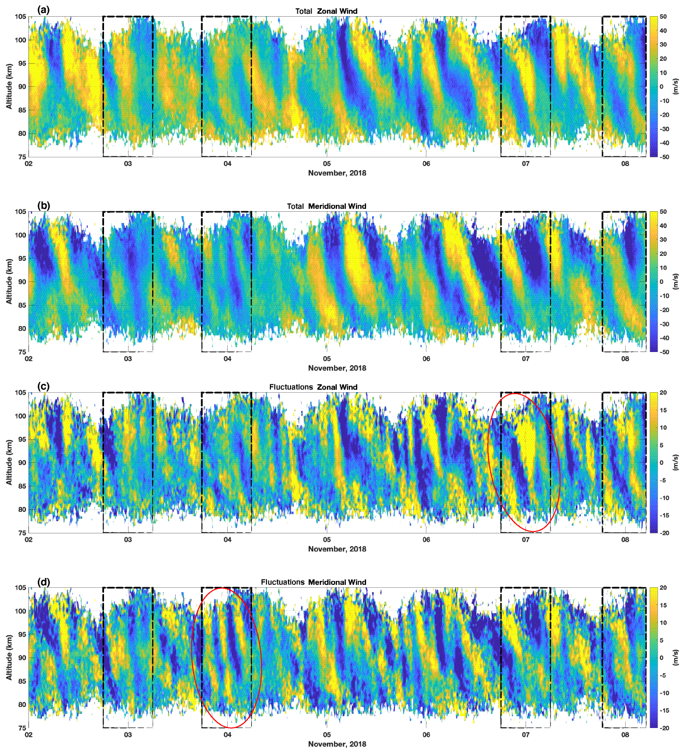
Figure 2(a) Zonal and (b) meridional wind measurements for the duration of the SIMONe–2018 campaign generated by the MSMR network. Note the dominance of the semidiurnal tide on the horizontal wind. (c) Zonal and (d) meridional wind fluctuations of τo ≤ 4 h. Note the presence of coherent gravity wave features (red ellipses) on 3–4 November in the meridional wind fluctuations and on 6–7 November in the zonal wind fluctuations coincident with enhanced keogram brightness for the same nights in Fig. 1. Dashed boxes indicate hours of simultaneous operation of the ASI and MSMR systems.
Here, we have used the MSMR winds in combination with the airglow data to give a full characterization of the gravity wave dynamics observed during the campaign. Figure 2 shows the (a) zonal and (b) meridional background winds in the range of 75–105 km measured during SIMONe–2018. Dashed boxes indicate hours of simultaneous operation of the ASI and MSMR systems. The background wind field is calculated from the MSMR measurements using 30 min temporal and 1 km spatial windows. Observe the daily cycle for z < 80 km and z > 100 km in the plots that is associated with the variation in meteor detections throughout the day; the meteor density is larger in earlier morning hours and smaller in afternoon hours. Because wind calculation relies on the number of meteors to make quality wind estimations, when not enough meteors are detected, the wind cannot be estimated within a reasonable uncertainty level. The background wind is dominated by a 12 h tidal oscillation presenting amplitudes larger than 50 m s−1, but spectral analysis reveals the presence of higher tidal harmonics of 8 and 6 h (see Figs. 6 and 7).
Figure 2c and d also present the zonal and meridional wind fluctuations associated with oscillations caused by gravity waves. To obtain the wind fluctuations, we first average the MSMR raw data over a 400 km2 field of view using a square 4 h temporal, 4 km vertical window. Then, we subtract the result from the background wind field. Note that oscillations of τo > 4 h and λz < 4 km will be suppressed but not completely eliminated in the resulting wind fluctuations. The fluctuation winds show short-period gravity waves perturbing the wind that are also seen in the airglow. For instance, the oscillation evident in the airglow brightness variation (red ellipse) for 3–4 November (Fig. 1c, meridional keogram) is also evident as coherent oscillations in meridional wind fluctuations (red ellipse) on 3–4 November (Fig. 2d).
2.3 Satellite data (TIMED-SABER)
We have also collected observations of the SABER instrument on board the TIMED satellite (Russell et al., 1999; Mlynczak, 1997) within 4∘ of the observation site (Fig. 3). The profiles cover the height range from approximately 10 km to more than 100 km. The vertical resolution is ∼ 2 km. The instrument covers ∼ 52∘ latitude in one hemisphere to 83∘ in the other in a given day. The viewing geometry alternates every 60 d due to 180∘ yaw maneuvers of the TIMED satellite (Russell et al., 1999). Approximately 1200 temperature profiles are taken each day. SABER publications are available at http://saber.gats-inc.com/publications.php (last access: 6 September 2021).
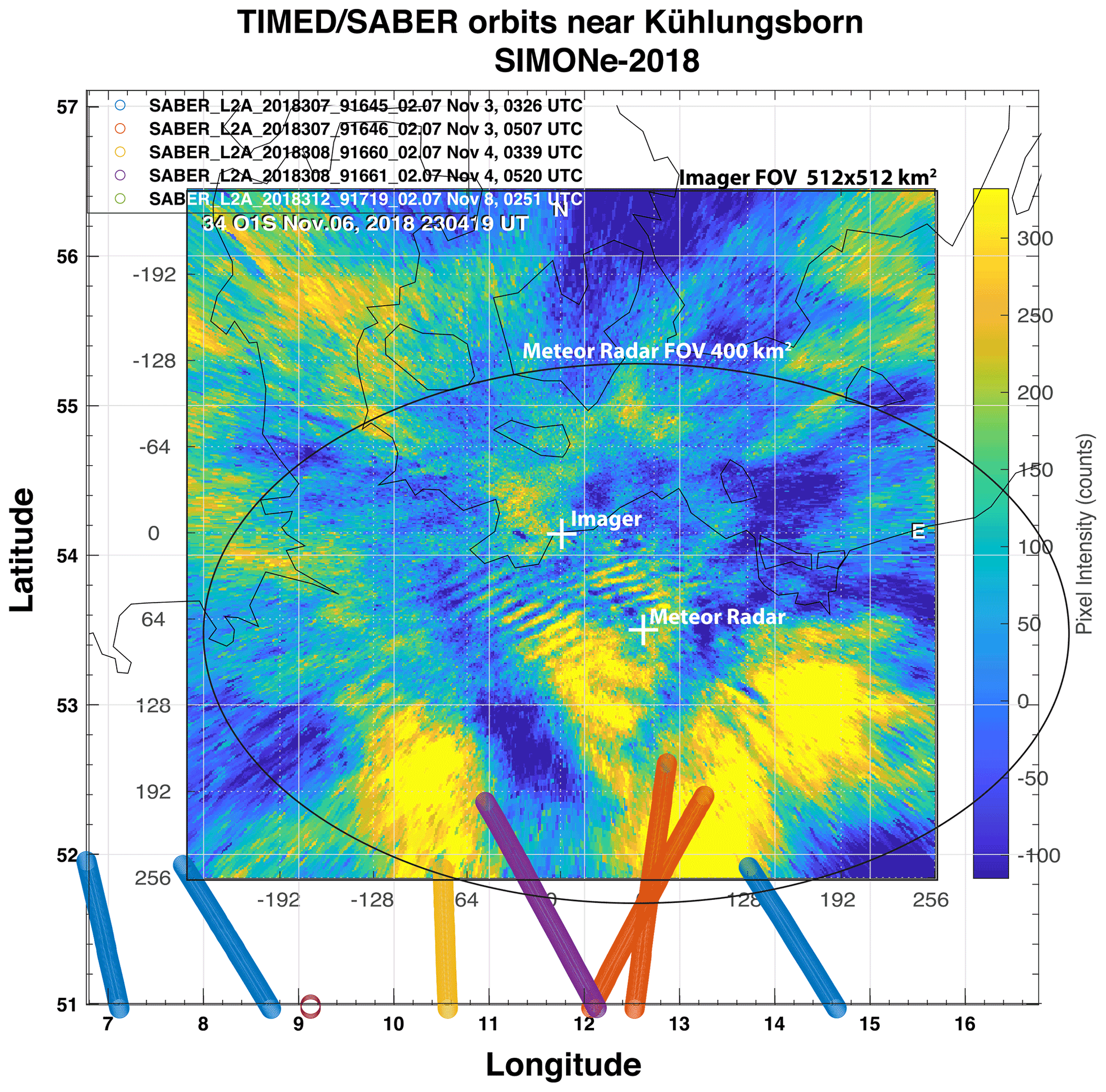
Figure 3Individual TIMED/SABER satellite orbits near Kühlungsborn during the SIMONe–2018 campaign. The colored lines represent the location where vertical atmospheric profiles were measured, not the actual satellite locus. The day and time of each orbit is indicated in the legend. The field of view of 512 × 512 km2 of the airglow camera projected at ∼ 95 km is indicated by the O(1S), TD image mapped onto geographic coordinates, while the ellipse indicates the field of view of the MSMR system. The white crosses indicates the coordinates of the imager system in the Kühlungsborn observatory and the meteor radar system.
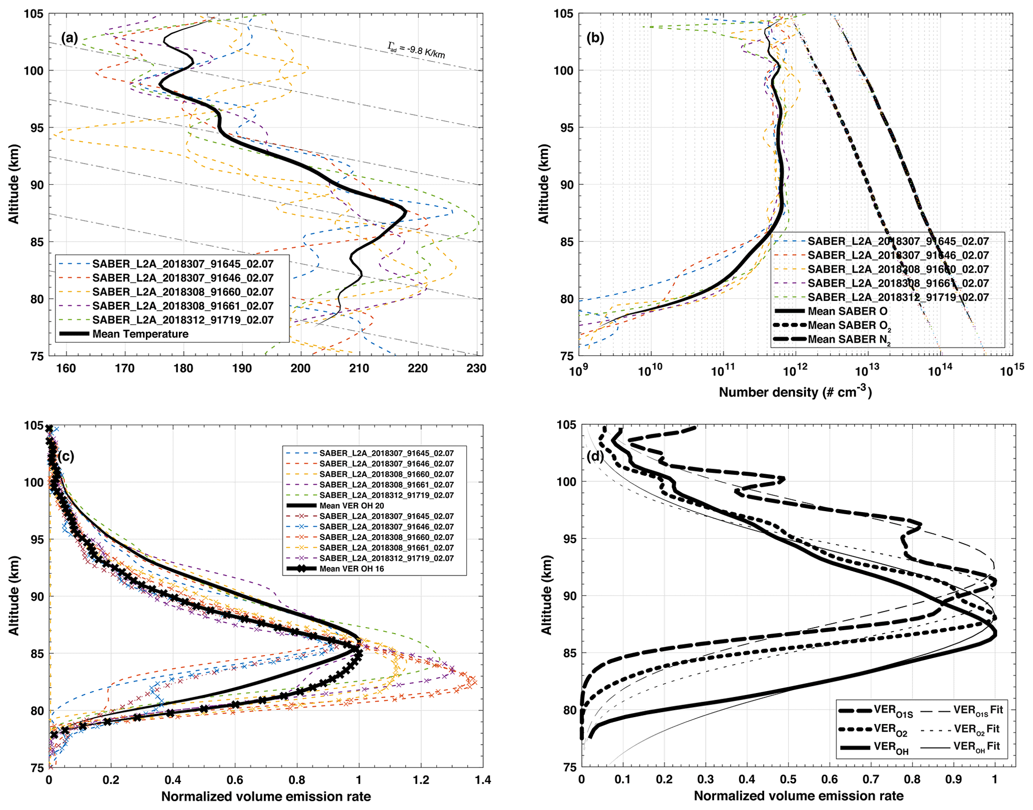
Figure 4(a) Temperature, (b) atomic oxygen, molecular oxygen, molecular nitrogen number densities, and (c) OH20 (2.1 µm OH(A)) and OH16 (1.6 µm OH(B)) volume emission rates collected by TIMED/SABER satellite near Kühlungsborn during the SIMONe–2018 campaign within 4∘ of latitude or longitude of the observatory. (d) Calculated volume emission rates for OH(8,3), O2(0,1), and O(1S) layers (thick black lines) using SABER mean profiles in panels (a) and (b). Colored dotted lines in (a), (b), and (c) indicate individual orbits of the satellite, while thick lines indicate the mean of the individual orbits. Gray dash–dot lines in (a) indicate the adiabatic lapse rate Γad = −9.8 K km−1. Thinner black lines in (d) are Gaussian fits of the calculated VER profiles. Individual VER airglow layer features for both measured and calculated VER are in Table 2. We have used SABER data version 2.07 to compose these plots.
SABER profiles used here are presented in Fig. 4a–c, while Fig. 4d shows the calculated volume emission rate of the mesosphere airglow emissions as explained below. The thick lines in Fig. 4 indicate the mean of corresponding individual profiles (dotted lines) for the various orbits of the satellite during the campaign. The corresponding orbits are specified in the legend of each chart.
From Fig. 4a, we can verify that the atmosphere is, on average, stable in the altitude range of 88–99 km since the atmosphere lapse rate ( K km−1) is larger than the adiabatic lapse rate ( K km−1) and is positive ( K km−1) below and above the 88–99 km range. Even though the satellite orbits registered during SIMONe–2018 were not exactly over the observatory, the instrument measurements are performed in the vertical limb plane that is near or within the field of view of the imager (Fig. 3). Note that the colored dots indicate where the measurements were made, not the satellite position. Thus, there is a good chance the background atmosphere above the observation site is similar to that indicated by SABER (Fig. 4), although the temperature might still be influenced by gravity waves once we have averaged only a few profiles. Because of that, we are confident using SABER background profiles to make inferences about the propagation conditions for the waves seen over the observatory.
Table 2Centroid, peak, and FWHM of the OH, O2, and O(1S) layers measured and calculated using TIMED/SABER data collected near Kühlungsborn during the SIMONe–2018 campaign.
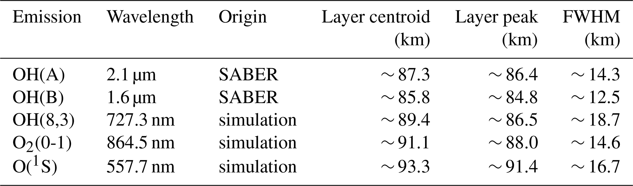
Figure 4d corresponds to our estimation of volume emission rate (VER) profiles for the OH, O2, and O(1S) airglow emissions. These VER profiles were calculated using the mean temperature, atomic oxygen, molecular oxygen, and molecular nitrogen profiles in Fig. 4a–b along with the reaction rates of each emission from Vargas et al. (2007). The characteristics of each layer (measured and calculated VERs) are obtained from a Gaussian model (thin lines in Fig. 4d) to fit each profile from which we obtain the layer peak, width, and the full width at half maximum (FWHM). The mean characteristics of the airglow layers are presented in Table 2. The goodness of fitting scores R2 > 0.95 for all five VER curves. The layer centroids, estimated from
are in general a few kilometers above the estimated layer peaks because of departures of the actual VER vertical structure from the Gaussian fitting model. We have simulated the VER profile for the OH(8,3) using the SABER mean temperature and atomic oxygen profiles for the campaign. The difference between the simulated OH VER and SABER OH VER lies on the averages used as inputs in the VER simulation. However, SABER OH VER and simulated OH VER are much closer in structure if we use individual SABER temperature and oxygen profiles.
A full characterization of the gravity wave field requires knowledge of the background wind over the observation site. The significant background wind acting in the vicinity of an airglow layer is a function of the vertical structure of the emission (the VER) that has finite thickness (see Fig. 4d). We take that into account by calculating the weighted background wind (Fig. 6a–c) by using the VER of each layer as weighting functions. The weighted wind expression for a given VER is
where uw and vw are the weighted zonal and meridional winds (Fig. 6), respectively.
3.1 Short-scale gravity wave analysis
We have defined here as small-scale the waves presenting λh < 725 km, while large-scale waves present λh > 725 km. This 725 km threshold corresponds to the length of the diagonal across the field of view of an airglow image mapped onto a 512 × 512 km2 grid. Thus, a 725 km horizontal-scale wave would present one crest and one trough fitting the image frame entirely. More details about raw airglow image preprocessing can be found in Appendix A.
The majority of waves observed during SIMONe–2018 are small-scale, fast oscillations of τi < 1 h. The keograms of Fig. 1 (right-hand side panels) show the most prominent waves of this category registered during the clear nights of the campaign. These short-scale gravity waves are analyzed here using the auto-detection method (Tang et al., 2005; Vargas et al., 2009; Vargas, 2019). The auto-detection method relies on three sequential airglow frames to obtain two time–difference images used in the cross-spectral analysis to obtain gravity wave parameters. The calculation of time–difference images leads to a change in the amplitude of the waves (in the TD images compared to the original ones). The amplitude influences the Fourier analysis and therefore also the result of the cross-correlation. However, this issue is properly taken care of by restoring the amplitude of the waves as seen in the original images. Further details about this correction and the auto-detection method are found in Appendix B.
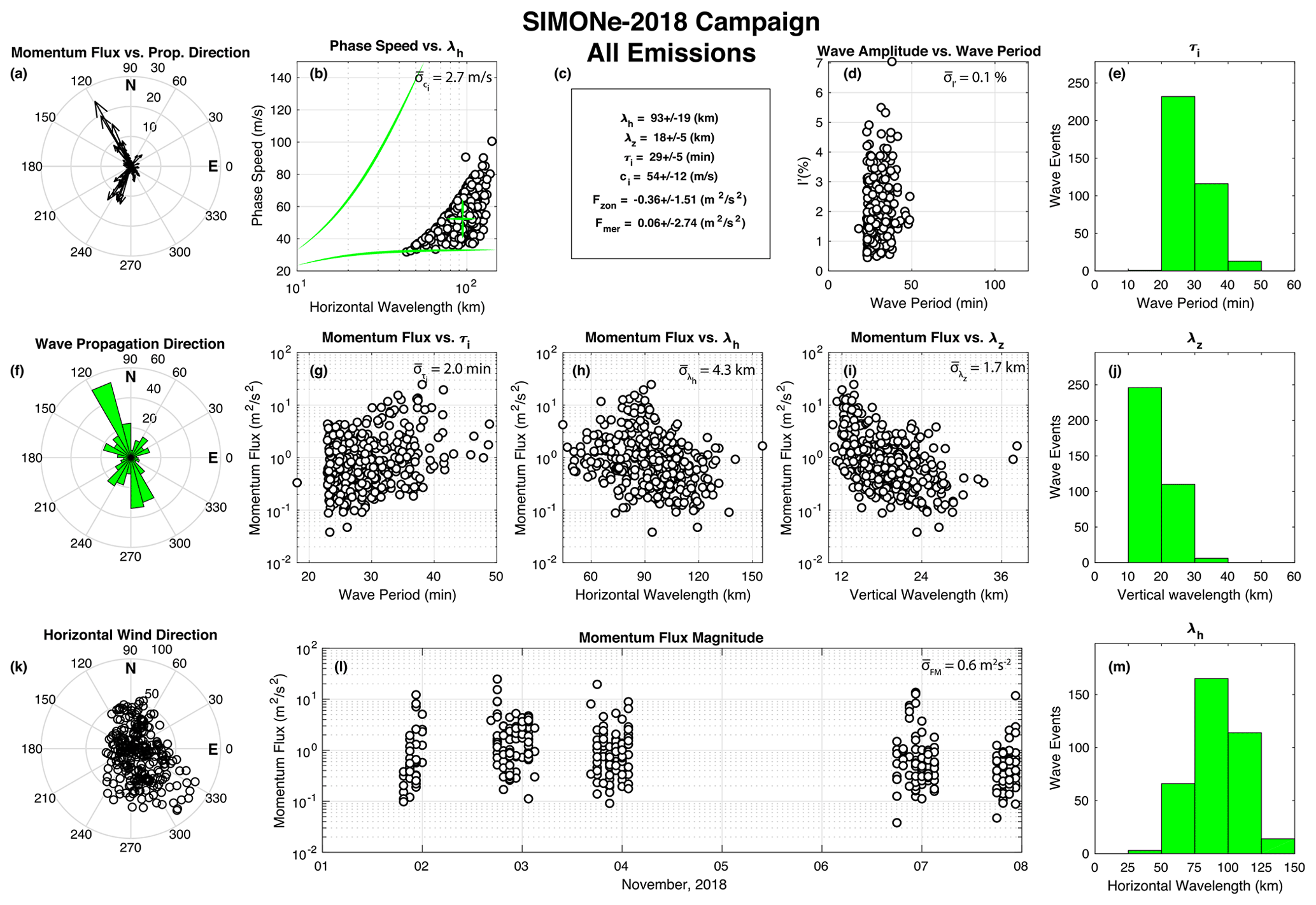
Figure 5Short-period wave parameters obtained from OH, O2, O(1S), and Na airglow image analysis using the auto-detection method (Tang et al., 2005; Vargas et al., 2009; Vargas, 2019). The mean measurement error is indicated in the chart of each wave parameter. Plots of waves detected in each emission separately are in the Supplement of this paper.

Figure 6(a) O(1S), (b) O2, and (c) OH volume emission rate weighted zonal and meridional background (unfiltered) winds. (d) O(1S), (e) O2, and (f) OH volume emission rate weighted zonal and meridional wind fluctuations. Wind fluctuations were obtained first by averaging the wind over 400 km2 field of view using a 4 h temporal, 4 km vertical window to obtain winds representing large-scales variations and then subtracting these estimates from the background wind field. The vertical blue arrows indicate coherent wind fluctuations also seen in the airglow brightness. Dashed boxes indicate hours of simultaneous operation of the ASI and MSMR system.
Figure 5 shows the results from the auto-detection method for all the emissions recorded during SIMONe–2018. Weighted background winds in Fig. 6a–c were used to carry out the Doppler shift correction on τo. Thus, the parameters shown correspond to intrinsic properties of the waves. We have calculated the error bars for the parameters of each wave event measured using the methodology in Vargas et al. (2019). The average error of each parameter is shown in their respective charts in Fig. 5. Since we rely on a set of three images at the time to compute the cross-spectrogram of a set, the time span of each set is about 20 min. It is possible that the observed wave events represent waves independent from one another because the observed waves have relatively long vertical wavelength and propagate vertically fast under weak horizontal winds. However, we recognize that this is not always the case, and, as the oscillations slow down as they propagate vertically, their residence time within a given airglow layer could be long. Therefore, some of the detected waves could have been counted twice while evaluating the average momentum flux and other wave statistics.
Because every image of a given airglow layer is taken at 10 min pace (the filter wheel cycle period), we are only able to resolve wave-apparent periods > 20 min. On the other hand, the exposure time used here is mostly 2 min; aliasing could be present due to this relatively long exposure time. However, we have assured the aliasing is minimal in this case because there is no smudging of the small-scale wave structures seen in the images.
The top-center box (Fig. 5c) contains a statistics summary of the measured wave parameters. Figure 5j shows λz ranging from 10 to 40 km, while λh in Fig. 5m clusters around 75–125 km. Waves transporting large FM are mainly oriented towards the northwest and southwest (Fig. 5a), but the polar histogram in Fig. 5f shows a large number of waves traveling southeastward into the dominant wind orientation (Fig. 5k). Estimated τi shown in Fig. 5e ranges within 20–40 min, with intrinsic phase speeds in the interval of 30–100 m s−1 during the campaign (Fig. 5b). The largest wave relative amplitude estimated from the images is 7 % in Fig. 5d, but this does not necessarily translate into large FM waves, which depends on other wave parameters.
Since the auto-detection method returns wave intrinsic parameters, we are able to estimate FM of every measured event (e.g., Vargas et al., 2007). Figure 5l shows the daily FM of waves detected during SIMONe–2018, with larger FM waves appearing on 2–3 and 3–4 November. The momentum flux vs. intrinsic wave period chart (Fig. 5g) reveals a tendency of larger τi waves carrying larger FM. Conversely, Fig. 5h (Fig. 5i) reveals that large λh (λz) waves associate with small FM quantities.
3.2 Large-scale gravity wave analysis
During SIMONe–2018, we also observed the presence of large-scale gravity waves modulating simultaneously the airglow brightness (Fig. 1c and e) and the horizontal wind (Fig. 2c and d). To study these large-scale oscillations in the wind at the altitude of the airglow, we have calculated the wind fluctuations weighted by the volume emission rate of each layer using
The result is seen in Fig. 6d–f, where the dashed boxes indicate hours of simultaneous operation of the ASI and MSMR systems.
The weighted wind fluctuations are similar in each layer as the layers peak within ±2 km from each other (see Table 2) and are thicker (mean FWHM ∼ 15 km) than expected (e.g., Greer et al., 1986; Gobbi et al., 1992; Melo et al., 1996; Wüst et al., 2017). The similarity of these fluctuations is related to larger-scale λz waves seen in Fig. 2c and d. Moreover, because the overlap of the VER profiles is non-negligible, the rms values of the weighted winds fluctuations are expected to have a similar magnitude. Calculated rms magnitudes are 6.9 ± 1.0 and 5.9 ± 0.9 m s−1 in the zonal and meridional directions, respectively.

Figure 7Spectra of weighted zonal and meridional wind fluctuation of Fig. 6. The dashed red lines indicate tidal periods. The vertical blue arrows indicate wave frequencies of persisting wave structures also seen in the airglow brightness. Statistical 99 % significance level is indicated by dotted blue lines.
The spectral content of the weighted wind fluctuations is shown in Fig. 7. Several tidal harmonics are still present in the spectra (vertical dotted red lines in Fig. 7). This is due to how the wind fluctuations are calculated, i.e., by first using a 4 h temporal, 4 km vertical window to obtain winds representing larger scales, then subtracting the result from the background wind. Thus, the obtained wind fluctuations will contain some of the energy of the tidal modes. However, there are persisting peaks attributed to gravity waves because of their presence in wind fluctuations and keograms. For instance, the peaks in Fig. 7 at the vicinity of 0.24 cycles h−1 are seen in the wind fluctuation of 3–4 November (meridional direction). Likewise, Fig. 7 shows a peak near 0.11 cycles h−1 corresponding to a wave of 8.9 ± 1.0 h also seen in the keograms of 6–7 November (zonal direction). A hodograph analysis of the winds must be carried out in a separate work to clarify the nature of the significant peaks in Fig. 7.
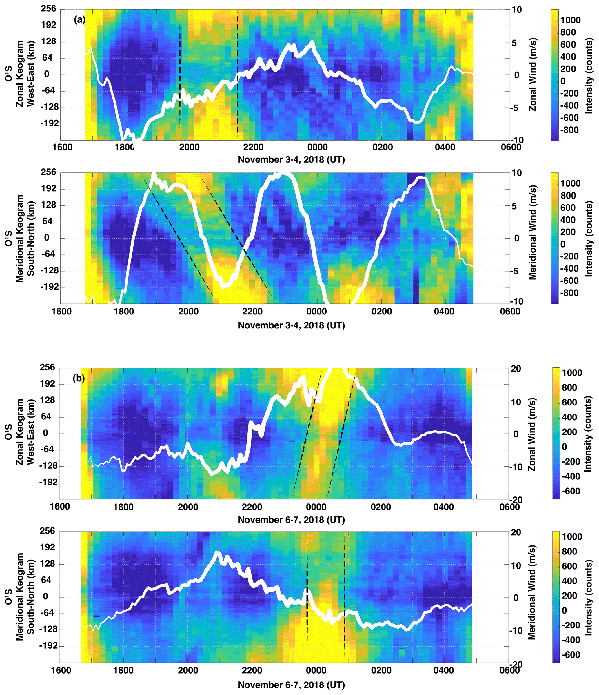
Figure 8Enhanced contrast keograms of O(1S) airglow for (a) 3–4 November and (b) 6–7 November 2018. The keogram of 3–4 November shows a large-amplitude, large-scale gravity wave at 20:00–22:00 UTC heading south. A large-scale wave is also seen on 6–7 November propagating eastward at 00:00 UTC. The white continuous lines on the keograms indicate the wind fluctuations weighted by the O(1S) volume emission rate.
We have studied further the wind fluctuations against obvious wave features present in the keograms of 3–4 and 6–7 November. By visual inspection of the images, we have verified that these large-scale waves do not fit within the airglow image field of view (512 × 512 km2) and are only noticeable via keogram analysis. We carry out the analysis by overlapping the O(1S) weighted wind fluctuations on top of the corresponding keograms for these nights (Fig. 8).
On 3–4 November (Fig. 8a), a strong and coherent oscillation is observed in the meridional wind fluctuation, while both zonal and meridional keograms present enhanced brightness structures around 21:00 UTC (dashed black lines). As the meridional wind fluctuation peaks, the meridional keogram brightness dims (Fig. 8a bottom); as the meridional wind fluctuation reverses direction, the airglow brightens. We have estimated τo ∼ 4.0 ± 1.0 h for this oscillation from the meridional wind fluctuations, where the assigned uncertainty in τo corresponds to the smallest division in the keogram temporal axis. The tilted brightness structure between 19:00 and 21:00 UTC in the meridional keogram indicates a wave is traveling southwards. The zonal keogram shows no obvious tilt in the enhanced brightness, suggesting no wave propagation in the east–west direction. That is confirmed from zonal wind (Fig. 8a top) that does not show any apparent oscillation in the same time span.
Similarly, we have observed enhancements in the airglow brightness on 6–7 November associated with a large-scale wave with τo ∼ 8.0 ± 1.0 h estimated from the wave activity in the zonal wind fluctuation seen in Fig. 8b top. The zonal wind fluctuation coincides well with the O(1S) enhanced brightness structure in the zonal keogram around 00:00 UTC. This brightness enhancement shows a slight tilt that indicates a wave propagating from west to east. The negligible brightness tilt in the meridional keogram (Fig. 8b bottom) implies the wave has no evident north–south component.
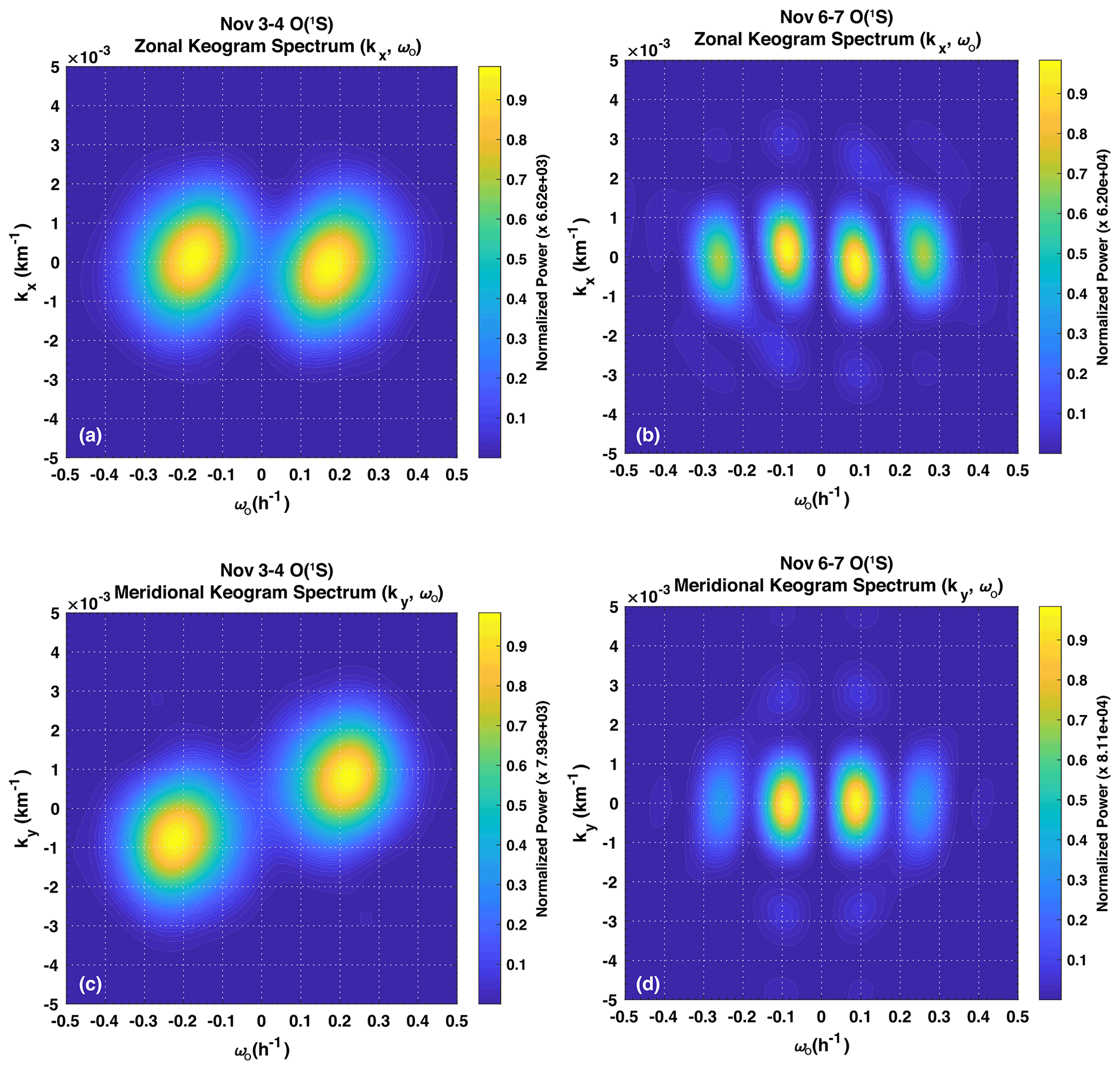
Figure 9Composite (kx,ωo) and (ky,ωo) spectra of the keograms in Fig. 8 for the nights of 3–4 November (a, c) and 6–7 November (b, d).
Spectral analysis of keograms for the two nights showing large-scale waves is shown in Fig. 9. The zonal and meridional keogram spectra for 3–4 November are in Fig. 9a and c, while zonal and meridional keogram spectra for 6–7 November are in Fig. 9b and d. Appendix C gives further details about the keogram spectral analysis carried out here.
For 3–4 November, the zonal keogram spectrum indicates a peak at kx=0 and cycles h−1 (τo = 5.7 ± 1.0 h), where the negative sign is associated with a forward-evolving time. The meridional keogram spectrum shows a dominant peak at cycles h−1 (τo = 4.6 ± 1.0 h) and cycles km−1 (λy ∼ 1365 ± 136 km), where the negative sign indicates a southward-propagating wave. The error in λy is based on Vargas (2019), who estimates 10 % error in measurements of large horizontal-scale waves (> 100 km) from spectral analysis. Note that because the horizontal scale of the wave in the meridional direction is twice as large as the mapped image field of view (FOV; 512 × 512 km2), the entire horizontal wave structure is hardly seen in a single airglow image but is doubtless recognized in the keogram.
The large-scale wave occurring on 6–7 November is represented in the zonal spectrum by the peak near cycles h−1 (τo = 9.1 ± 1.0 h) and cycles km−1 (λx ∼ 4096 ± 409 km), where the positive sign indicates an eastward-propagating wave. The meridional keogram spectrum indicates a peak at the same frequency but ky∼0, indicating no wave propagation in the meridional direction.
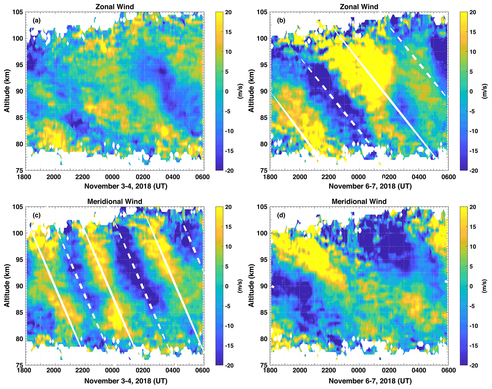
Figure 10Time–altitude cross section of the zonal and meridional wind fluctuations for the nights of 3–4 and 6–7 November 2018. The continuous (dashed) white lines indicate crests (troughs) of the oscillations as well as the descending phase (ascending energy propagation) of the waves. Note the coherent τo ∼ 4.3 h gravity wave oscillation on 3–4 November with λz ∼ 25.6 km. The zonal wind oscillation on 6–7 November corresponds to a λz ∼ 21.3 km, τo ∼ 8.0 h gravity wave.
Figure 10 shows the time–altitude cross section of the zonal and meridional wind fluctuations for the nights of 3–4 and 6–7 November, respectively. The descending phase progression in time–altitude cross section reveals that these large-scale waves are propagating upwards. We have drawn continuous (dotted) white lines on top of the crests (troughs) of the salient wave structures to estimate λz and τo of the oscillations. The lines were drawn where the wave structures are better defined on top of the meridional wind (3–4 November) and zonal wind (6–7 November) fluctuation cross sections. From these lines, we have estimated λz = 25.6 ± 1.0 km and τo = 4.3 ± 1.0 h for the wave seen on 3–4 November. Note that the assigned error of 1 km in λz corresponds to ∼ 2 times the vertical resolution of the vertical axis in Fig. 10, while the assigned error of 1 h in τo corresponds to the resolution of the temporal axis in Fig. 10.
For the wave seen on 6–7 November we have obtained τo = 8.0 ± 1.0 h and λz = 21.3 ± 1.0 km. This long-period wave is not related to the 8 h tide since the horizontal structure of the oscillation can be seen in the keogram of Fig. 8b entirely. The apparent periods derived here from the descending phase analysis are consistent with those from the keogram spectral analysis shown earlier.
The propagation conditions for gravity waves during SIMONe–2018 are depicted in Fig. 4 showing the temperature and constituent densities near the Kühlungsborn observatory. While the vertical structures of the atomic oxygen density appear normal, the mean temperature indicates convectively favorable conditions for gravity wave vertical propagation as the ambient lapse rate is positive for 87 km and 99 km. Within the 88–98 km range, the ambient lapse rate is negative but still sub-adiabatic, and convective instabilities are unlikely to form under these conditions. Thus, gravity wave dissipation due to convective instabilities would not affect the vertical evolution of the gravity wave field during the campaign. We have also verified that dynamic instabilities did not occur because the wind shear was < 30 m s−1 km−1 most of the time during the campaign. On the other hand, because the horizontal winds occasionally achieved relatively large magnitudes > 50 m s−1 (Fig. 2a and b), the wind field could have caused absorption of waves having a phase speed < 50 m s−1 traveling in the same direction of the background wind.
We can verify the effect of background wind on the propagation direction of the waves by examining Fig. 5. The momentum flux vs. propagation direction chart (Fig. 5a) shows a number of waves with large FM oriented towards the northwest and southwest, while Fig. 5k shows a dominant southeastward wind during SIMONe–2018 observations. Thus, it is likely that the background wind controls the propagation of southeastward waves via dynamic filtering. However, the wave propagation direction histogram (Fig. 5f) indicates that a significant number of waves still propagate into the wind. These waves must then have a horizontal phase speed larger than the background wind. In fact, we have estimated an average ci = 56.6 ± 13.6 m s−1 for waves traveling in the southeast quadrant sector (270 to 360∘), while wind has a mean magnitude of 39.3 ± 18.9 m s−1 in the same sector (Fig. 5k. This suggests these fast waves were able to overcome absorption levels while propagating vertically.
Horizontal and vertical wavelengths, intrinsic periods, and intrinsic phase speeds of waves detected during SIMONe–2018 are directly comparable with the results of Li et al. (2011), who used a similar auto-detection method to analyze short-period, fast gravity waves in the airglow. Our statistics show an average λz of 18.5 ± 4.6 km (4.6 km is the sample standard deviation), which is compatible with the results of Li et al. (2011) showing λz clustering from 20 to 30 km. They have shown λh clustering around 15–30 km, while our results peak around 75–100 km. Fast waves reported here present remarkably larger horizontal scales than those of Li et al. (2011), which could be associated with the location and type of terrain (Maui – sea vs. Kühlungsborn – land) and gravity wave sources acting near the observatories. Yet, our sample is representative of the winter solstice conditions observed during a week, while that from Maui is representative of the season conditions observed over 5 years.
There are obvious discrepancies in τi estimated here compared to those of Li et al. (2011). Observe that τi here bulks around 20 to 30 min, while Li et al. (2011) report 77 % of waves having τi < 10 min. We attribute this discrepancy to the different integration time and the filter wheel cycle of the observing airglow camera systems; during SIMONe–2018, we have observed several emissions using a filter wheel cycle period of 10 min, which only allows us to detect waves presenting τo > 20 min. Li et al. (2011) used a filter wheel cycle of 2 min while observing a single emission, allowing the detection of waves of timescales as short as ∼ 5–6 min, near the Brunt–Väisälä period. The filter wheel cycle time seems to affect other parameters as well. For instance, while Li et al. (2011) report a majority of wave intrinsic phase speeds in the range of 50–100 m s−1; we have estimated slower intrinsic phase speeds of 31.2 ± 17.3 m s−1. The filter wheel cycle influences the sensitivity of the measurement system in the temporal domain but not the spatial domain, that is, the system will automatically detect faster waves having smaller-periods but in the same λh range.
In another study, Li (2011) used 1 year of OH airglow observations over the Andes Lidar Observatory (ALO) in South America to characterize small-scale, fast gravity waves. He found that the peak of distribution of λh falls in the 20–30 km range, ci ranges mainly 40–100 m s−1 (peak at 70 m s−1), 80 % of the τi population ranges from 5–20 min, and the λz distribution peaks around 15 km. These results resemble those of Maui, and the same discrepancies are applicable for the results in SIMONe–2018. However, the sources of waves over the South American observatory are much clearer and related to convection in central Argentina to the east of ALO. These sources generate fast, short-period, small horizontal-scale waves that can be captured over the ALO imager. The farther away the source, the fewer short-periods waves are seen, which explains a secondary peak around λh = 80–100 km shown in Li (2011). This range is comparable to the λh distribution from the SIMONe–2018 campaign showing a peak around λh = 75–100 km that would be related to tropospheric convective sources active to the north and east of Kühlungsborn during SIMONe–2018.
The momentum flux of high-frequency waves detected during SIMONe–2018 (Fig. 5) is calculated using Vargas et al. (2007, Eq. 13) as shown in Appendix B. The mean momentum flux has a larger component towards the west of −0.36 ± 1.51 m2 s−2. Note that the mean FM shows a tendency of a net wave motion westward, while the standard deviation indicates that waves could be moving westward or eastward. The FM meridional component is ∼ of the zonal magnitude. Ignoring for a moment the wave propagation direction, the mean FM = 1.62 ± 2.70 m2 s−2. For all the 362 waves detected during SIMONe–2018, 50 % of the total FM is due to waves carrying FM > 3 m2 s−2 (40 events); that is, only 11 % of the detected waves are responsible for 50 % of FM measured during the campaign. This result agrees with the findings of Cao and Liu (2016) that show most of FM is due to waves that occur very infrequently (low intermittency). However, Cao and Liu (2016) also conclude that small FM waves are important because of their higher occurrence rate.
Observe that the 362 detected events are not necessarily independent, that is, the same wave could have been detected multiple times throughout the night. However, we rely on sets of three images to make wave detections. Since the time span of each set is about 20 min (10 min between successive images), waves detected in the given set would have disappeared from the imager FOV after that time span. This is because the duration of quasi-monochromatic wave packets in airglow images are generally short. Thus, the same waves are unlikely to be detected in multiple image sets. This way, it would be more likely that most of the 362 detections correspond to different, independent waves.
In spite of the small mean value, FM bursts between 10–30 m2 s−2 were mainly seen in the O2 emission during the campaign. These waves were traveling northwestward with τi = 30–40 min, λh ∼ 90 km, and λz = 12–15 km (see charts of each emission in the Supplement). The sum of FM of these waves (eight events) accounts for 20 % of the total small-scale wave FM measured during the campaign. It is not clear why the enhanced waves are seen most in the O2 emission once the layer's peaks nearly overlap, but this could be related to the O2 VER having a narrower FWHM (see Table 2). This way, shorter λz waves would be detected primarily in O2 images, presenting larger FM since it increases as λz decreases (Fig. 5i).
We see that even in smaller numbers, the more energetic, larger FM waves could have a greater impact in the atmosphere. For instance, during the Deep Propagating Gravity Wave Experiment (DEEPWAVE), Bossert et al. (2015) investigated mountain waves presenting horizontal scales of 200–300 km with FM in the range of 20–105 m2 s−2. Similarly, Smith et al. (2020) estimated FM ∼ 232 m2 s−2 associated with an extensive and bright mesospheric gravity wave event seen over the El Leoncito Observatory, Argentina (31.8∘ S, 69.3∘ W), during the nights of 17 and 18 March 2016. The waves observed in this study carrying FM > 3 m2 s−2 would potentially cause FD ∼ 22–41 m s−1 d−1 (Vargas et al., 2007, Fig. 9e), considering that the wave breaking continues for 24 h. This would lead to considerable mean flow deceleration and body forces capable of exciting secondary waves as point-like sources (Vadas and Becker, 2018). Considering the wave source and wave breaking mechanism acting for 4 h (about half of a typical nighttime observation period) at a given altitude, we estimate a potential mean flow deceleration of 3.7–6.8 m s−1 in this time span (4 h) due to wave forcing.
In a similar study, Suzuki et al. (2010) presented identical gravity wave structures detected in airglow intensity, radar wind, and lidar temperature. In airglow keograms from Northern Hemisphere stations in Japan, they observed small-scale gravity waves with λh ∼ 170 km, a period of 1 h propagating northeastward at ∼ 50 m s−1. Using from both airglow images and meteor radar wind, they calculated an average FM of 0.8 m2 s−2 at 94 km and 1.5 m2 s−2 at 86 km for the observed oscillations. The Suzuki et al. (2010) flux measurements agree with our estimates for small-scale waves that show a majority of events carrying small FM. They have also estimated the acceleration of 0.8 m s−1 h−1 (19.2 m s−1 d−1) at the 94 km height, which is close to our estimations of FD for small-scale waves.
Ern et al. (2011) shows absolute FM values of ∼ 10−3.9 Pa at 50 km altitude and ∼ 10−4.3 Pa at 70 km altitude in the Northern Hemisphere in January for latitudes/longitudes near the Kühlungsborn observatory, evidencing momentum flux deposition in the middle atmosphere. Thus, it is likely that the small-scale waves observed here mostly dissipate as they travel through the MLT, in agreement with Vargas et al. (2019). In another flux estimation study using airglow imagery of gravity waves, Vargas et al. (2009) revealed FM ranging from ∼ 1.5 to ∼ 4.5 m2 s−2, while radar measurements of, e.g, Yuan and Fritts (1989) estimated FM = 5–15 m2 s−2. Also, it is believed 70 % of the momentum is carried by short-period waves (< 1 h) (Vincent, 1984). Estimations of FD (wave drag) in the meridional direction from airglow measurements unveiled accelerations of 3 m s−1 d−1 (Vargas et al., 2015), which is significant given that the meridional wind magnitude is weak (∼ 20 m s−1 or less at midlatitudes), while in the zonal wind the wave FD = 15–60 m s−1 d−1 (Vincent and Fritts, 1987).
We have also estimated the horizontal wavenumber and apparent frequency of the large-scale waves shown in the airglow (Fig. 8) from the spectrum of the zonal and meridional keograms in Fig. 9. We then estimate λz of the events assuming a Brunt–Väisälä period of 5.5 min (N=0.01904 rad s−1) and an inertial period of 14.8 h ( rad s−1) for the Kühlungsborn latitude. We use the acceleration due to gravity g=9.5 m s−2 for the mesosphere.
The wave occurring on 3–4 November presents cycles km−1 and ωo=0.215 cycles h−1 estimated from the keogram spectra. The weighted background wind field over the observatory at 23:15 UTC presented u=28.5 m s−1 and m s−1 at the instant the wave was in the dimmer phase of its cycle in the airglow. Then applying a Doppler shift correction, we estimate an intrinsic frequency ω=0.211 cycles h−1 for the wave. Finally, using the dispersion relation (Appendix C), we derive km for the 3–4 November wave, where the uncertainty is 20 % as estimated in Vargas (2019). This wavelength compares well with km obtained by visual inspection of Fig. 10.
Likewise, the 6–7 November wave has cycles km−1 and ωo=0.11 cycles h−1. Applying once again the Doppler shift correction using background wind components of u=26.0 m s−1 and m s−1 at 23:26 UTC, we obtain an intrinsic frequency of ω=0.087 cycles h−1. From the dispersion relation we then estimate km for this wave, which also agrees with the measured value of km from Fig. 10.
The amplitudes of the large scale from keogram waves are = 36.5 % (3–4 November @ 21:30 UTC) and = 47.9 % (6–7 November @ 00:30 UTC). These amplitudes are relative to the mean airglow brightness of each night. As demonstrated in Appendix B, the vertical wavelength of each wave along with their perturbations in brightness permit us to evaluate their relative perturbation in temperature as = 9.1 % (3–4 November) and = 13.7 % (3–4 November ). Then, we finally estimate FM (see Appendix B) by using the intrinsic parameters found for the observed large-scale waves, which are FM=21.2 m2 s−2 for the wave seen on 3–4 November and FM=29.6 m2 s−2 for that seen on 6–7 November. Table 3 shows a summary of the main features of the large-scale waves as discussed above. We expect the uncertainties in FM to be large (> 40 %) given that the FM variables incur in uncertainties that are transferred to FM via error propagation (Vargas, 2019).
Table 3Estimated features of the large-scale waves observed in the airglow and meteor radar wind data.

Based upon FM values of the large-scale waves, we estimate for the southward-traveling wave (3–4 November) a momentum flux divergence FD ∼ 43 m s−1 d−1 in the meridional flow, assuming this wave breaks or dissipates at a given level along its vertical path. Similarly, the 6–7 November wave would cause a deceleration of FD ∼ 38 m s−1 d−1 in the zonal flow at the breaking or dissipation level. These large-scale, large-amplitudes waves would have a greater impact on the mean flow than small-scale waves, even though these waves are less frequent in mesospheric measurements than their small-scale counterparts.
Gong et al. (2019) also investigate the properties of large-scale, long-period waves observed on 30 May 2012 in China. Datasets of three instruments used in the study have shown evidences of the same gravity-wave-perturbing lidar and SABER temperatures as well as meteor radar winds. The parameters associated with the observed wave are λh = 560 km, λz = 8–10 km, τo = 6.6–7.4 h, and a phase speed of 21 m s−1. Gong et al. (2019) and Reichert et al. (2019) along with our study represent a few efforts to characterize larger-scale gravity waves propagating from the stratosphere into the mesosphere using multi-instrument datasets.
According to Vargas et al. (2019), only a minority of waves seen in the airglow (∼ 5 %) are in non-dissipating regimes. Vargas et al. (2019) also show that the majority of the gravity waves present strong dissipation and transfer momentum flux to the main flow within a distance of two atmosphere-scale heights (12–14 km). Thus, the large FM waves discussed here are likely to present dissipative or breaking characteristics given their larger amplitudes. This is not without controversy, since recent radar measurements in Antarctica (Sato et al., 2017) have shown longer-period gravity waves (1 h–1 d) transporting larger FM, although short-period oscillations also have significant FM but are relatively smaller.
Recently, Vadas and Becker (2018) have modeled the evolution of mountain waves over the Antarctic Peninsula after observational results of large-scale, long-period waves seen in the mesosphere (Chen et al., 2013, 2016) attributed to an unbalanced flow in the lower stratosphere. This imbalance excited upward- or downward-propagating oscillations from the knee of fish-bone-like structures at 40 km altitude, which are associated with the excitation of secondary waves from the breaking of extensive mountain wave structures. Although other modeling efforts also attribute the excitation of non-primary waves to localized turbulence eddies from gravity wave breaking (e.g., Heale et al., 2020), we believe that the large-scale waves observed in this study are the product of the Vadas and Becker (2018) mechanism at play in the stratosphere. In fact, preliminary analysis of temperature profiles at 0–90 km altitude acquired by the IAP Rayleigh lidar system on 6–7 November revealed fish bone structures at 40–45 km, resembling the predictions of Vadas and Becker (2018). We will investigate in detail the possible connection with the large-scale waves seen here in a separate paper; specifically, we want to identify potential sources of primary waves in the vicinity of Kühlungsborn during SIMONe–2018 and also trace the observed large-scale waves back to their excitation altitude around the fish bone knee region at 40–45 km revealed in the filtered lidar temperatures.
In this paper, gravity waves of small and large horizontal scales were characterized by their intrinsic wave parameters, amplitudes, momentum fluxes, and momentum flux divergences. We have focused the analysis on data recorded simultaneously by an airglow all-sky camera, multistatic specular meteor radar, and TIMED/SABER satellite to obtain a more extensive collection of complementary information about the state of the mesosphere region over the observatory during the campaign. To uncover small horizontal-scale features, we have used an auto-detection method to process all-sky airglow images and background meteor radar winds. Large-scale waves were characterized by spectral analysis of airglow keograms and an altitude vs. time cross section of wind fluctuations.
Our results indicate that 11 % of all detected gravity wave events have large amplitudes and carry 50 % of the total FM estimated during SIMONe–2018. These fewer wave events could impart mean flow deceleration of FD = 21–43 m s−1 d−1 towards the wave propagation direction at breaking or dissipation levels. We have estimated FD using Vargas et al. (2007, Fig. 9e) results for waves having λz = 20–25 km and λh > 100 km. However, the deceleration will be smaller because the waves are unlikely to be breaking or dissipating continuously for 24 h, dying out earlier.
Given the relatively large λz and λh of the observed large-scale waves, there is a possibility that these events are the product of secondary wave excitation via the mechanism identified by Vadas and Becker (2018). This possibility is supported by stratosphere fish bone structures uncovered in filtered temperatures collected over Kühlungsborn with the IAP Rayleigh lidar system on 6–7 November. A complete analysis of these structures will be given in a separate paper, in which we also plan to show the origin of the primary waves in the troposphere from weather images as well as the presence of non-primary waves in other datasets such as that of the Atmospheric Infrared Sounder (AIRS) on board the AQUA satellite.
For a given observation night, in the absence of contamination sources (e.g., cloudiness), a series of airglow images is produced by our airglow imager system with 10 min per image and ∼ 2 min integration time. Prior to spectral analysis being carried out, each raw airglow image must pass through a series of preprocessing steps. First, the image frame is centralized such that the image zenith coincides with the central pixel of the image frame. Second, the image is rotated and flipped over such that the image top points northward and the image left points eastward. Third, the stars are removed using a star suppression algorithm (Tang et al., 2005). Fourth, the resulting image is then mapped onto a geographic plane of 512 × 512 km2 projected at the height of the emission layer (Garcia et al., 1997). Fifth, the images are detrended by subtracting a fitted linear surface from the image frame. After these preprocessing steps, the resulting frames are then uniform across the FOV with a pixel resolution of 1 km per pixel and ready for spectral analysis (auto-detection or keogram spectral analysis methods) to obtain gravity wave parameters present in the images.
The auto-detection method for image processing and analysis was used in this study to obtain parameters of quasi-monochromatic waves from sequences of airglow images. This process detects waves and estimates its parameters automatically, making the study of gravity waves more effective, especially in relation to the estimation of FM. Compared to conventional techniques, which involve looking for waves from the visual inspection of preprocessed image sequences, this method is more optimized because it processes a set of three images at a time, requiring relatively less processing time.
The FM carried by vertically propagating waves is estimated from intrinsic parameter waves, knowing the prevailing wind calculated from meteoric radar data. Preprocessed images mapped in a 512 × 512 km2 grid are cropped around the zenith to produce the 174 × 174 km2 analysis window because the central region of the image is less sensitive to lens distortion.
The method automatically corrects τo Doppler shift due to the background wind. This is done by shifting the image pixels of each direction by a distance proportional to the wind velocity divided by the image acquisition period (Tang et al., 2005). Pixel shifting is performed in the first and last images of a set. The corrected set is used to compose two TD images. A TD image is produced by subtracting an image from the previous one in the image set (Swenson and Mende, 1994; Swenson and Espy, 1995; Tang et al., 2005; Vargas, 2019).
Two TD images are generated from sets of three consecutive preprocessed airglow images around a given instant. The Fourier transform is applied to each TD image, and the cross-spectrum is then obtained from the individual TD spectra. Thus, the spectrograms of each TD image are obtained from the 2D fast Fourier transform (FFT) and are combined to form the cross-spectrogram of the image set (e.g., Vargas, 2019).
Let J1(kx,ky) and J2(kx,ky) be the Fourier transforms of two TD images from a given set. In general, lateral lobes associated with spectral peaks appear in the spectrogram as a result of the limited spatial extent of the image. In this work, we applied the 2D Hanning window in the TD images to minimize the lateral lobes while preserving the energy of sinusoidal components associated with gravity waves. The cross-spectrogram is described in terms of both J1(kx,ky) and J2(kx,ky) as
where the asterisk designates the complex conjugate and n2 the number of pixels in the image. The cross-spectrogram contains information about the wavenumber, temporal frequencies, and the phase difference of the dominant components of the spectrum.
The dominant wavenumbers of the image set are then identified from the amplitude cross-spectrogram , while the dominant wave periods are determined from the phase cross-spectrogram. The wavenumbers kx and ky are determined at the location of the ith spectral peak to obtain , providing . The wave orientation is then .
From the phase cross-spectrogram we obtain the phase shift δθ of the wave between TD images at the location of the spectral peak (kx,ky). We now can estimate the ci of the wave using
where δt=10 min is the filter wheel cycle period. The intrinsic wave period is then found from . Note that at this point, the wave propagation direction ϕ has an 180∘ ambiguity. This ambiguity is resolved by taking the (kx,ky) pair values from the phase cross-spectrogram where δθ<0, which corresponds to a time coordinate progressing forward.
The airglow brightness I detected by the CCD sensor can be regarded as the superposition of a basic state and a state disturbed by waves I′ such as . Again, I′ is estimated in the wavenumber domain based on the amplitude cross-spectrogram. The undisturbed component , on the other hand, is obtained by the mean airglow brightness over the image field of view.
The relative wave amplitude in intensity over the FOV is estimated by integrating the energy around a given spectral peak. The wave information is only stored if has energy > 10 % of the total cross-spectrogram energy. The basic hypothesis for restoring the wave energy is that the wave content throughout the image is uniform. However, the animation of TD images reveals that monochromatic waves do not always cover the entire FOV; thus, the energy extracted from the wavenumber domain represents an average wave energy over the FOV. The size of the analysis window (174 × 174 km2) is important because it is small enough to allow the wave event to cover the entire FOV, giving a more accurate estimate of its energy, and large enough to ensure the detection of waves in the range of 2–174 km. Note that while this procedure restricts the field of view, dynamic parameters of gravity waves can be estimated more reliably since the full wave structure is captured by this smaller analysis window.
The TD image operation affects the amplitude of the waves of different periods according to the following equation:
where is the wave amplitude after the TD operation is carried out and δt is the image acquisition time. Figure B1 shows this effect where short-period waves will be amplified () while long-period waves will be attenuated (). The amplification range lies within min. Prior to carrying out other wave parameter estimation, we have to obtain the real wave amplitude. Figure 11 shows a filtering effect intrinsic to the auto-detection method that limits the observation of waves having periods that are harmonics of the acquisition time (that is, 10 min, 5 min). Observe in Fig. 11 that the amplitude decays fast for waves with a period < 20 min and becomes zero for a period equal to 10 min. Ideally, a better airglow experiment would rely on having individual all-sky imagers dedicated to individual emissions. Having a higher time resolution between sequential images is ideal, but this cannot be accomplished in most of the airglow observatories. This difficulty manifests here as the auto-detection method's inability to capture waves of periods shorter than the integration time, making our results restricted to a subset of observable gravity wave periods.
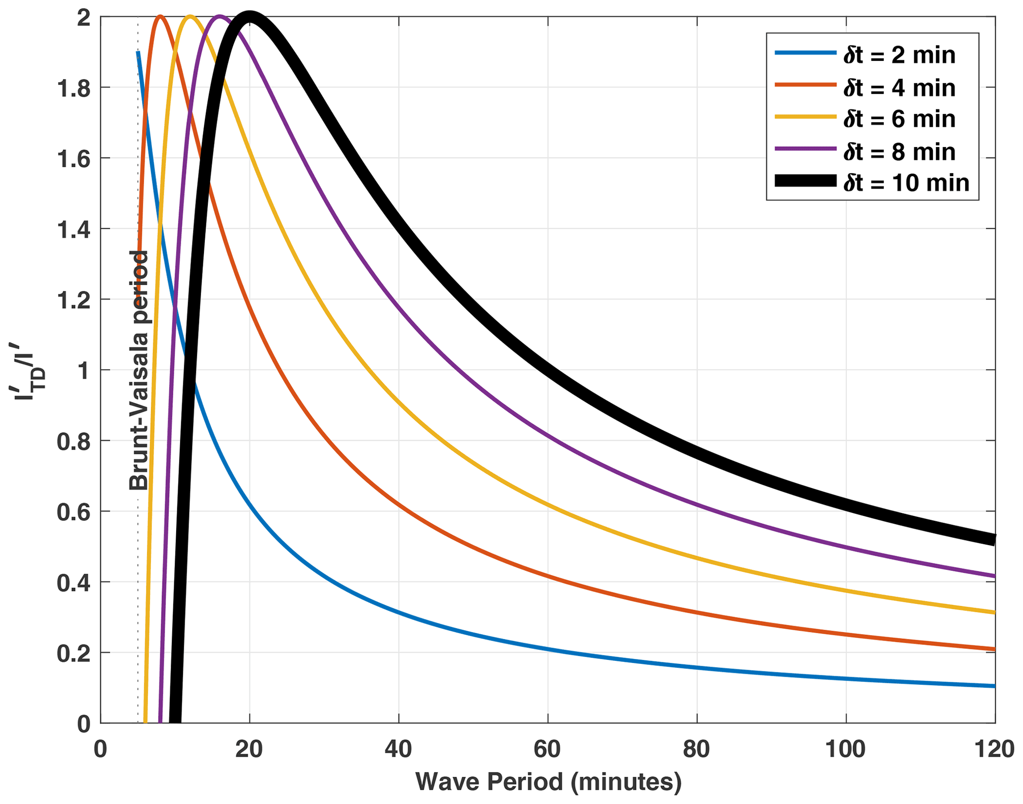
Figure B1Effect of time difference image filter on gravity wave amplitudes of various periods and acquisition times (δt). The thick black line corresponds to the acquisition time of our imager during SIMONe–2018.
We then evaluate using the complete gravity wave dispersion relation
where is the ratio of specific heats and H is the scale height in the MLT, while g and N are the acceleration due to gravity and the Brunt–Väisälä frequency, respectively.
The momentum flux is calculated using (Vargas et al., 2007, Eq. 13)
where ω, kh, m, , g, and N are the wave angular intrinsic frequency, horizontal wavenumber, vertical wavenumber, percent temperature fluctuation, acceleration due to gravity, and the Brunt–Väisälä frequency, respectively. The percent temperature fluctuation is calculated using the cancellation factor (Vargas et al., 2007, Eq. 12)
as the relative wave amplitude in intensity is obtained from the amplitude spectrogram as described earlier.
The operations above run in a loop that iterates continuously for the number of images collected in a given observation night. The wave parameters, their uncertainties, and the occurrence time stamps of the events are stored in a separated file for each night.
While individual airglow images represent a routine way to study short-period, small-scale gravity waves, keograms are conveniently used in this study to investigate the characteristics of major low-frequency, large-scale oscillations, revealing wave activity over the time span of the observation night.
We built zonal (meridional) keograms by taking the central row (column) of raw or preprocessed airglow images collected in a given observation night (Vargas et al., 2020). In the zonal keogram, the vertical scale indicates west (negative) and east (positive), while the vertical scale in meridional keograms indicates south (negative) and north (positive). The horizontal scale in both zonal and meridional keograms refers to universal coordinated time (UTC). Note that the center of vertical axis of the keograms corresponds to the brightness registered by the zenith pixel localized at the center of the images.
Large- and small-scale waves show up in keograms as tilted luminous or dark patches. The deeper the tilt is, the slower the phase speed (long τo) of the wave (Vargas et al., 2020). The horizontal wavelength can be also determined from keogram images as long the wave has a nonzero phase speed at least in a given direction (zonal or meridional). The wave tilt angle is measured from the horizontal axis to the wave luminous patch in the keogram and is positive if the wave travels eastward (northward) in the zonal (meridional) keogram.
Zonal and meridional keograms are airglow brightness time series as a function of zonal and meridional distances. The temporal axis has a resolution of 10 min and the spatial axis (zonal and meridional) has a resolution of 1 km per pixel. Thus, waves presenting τo > 20 min and λh > 2 km can be resolved by this method. The spectral analysis of keograms is carried out in the Fourier space via 2D-FFT preceded by Hanning windowing. The spectral content of the zonal (meridional) keogram can be seen in Fig. 9a (Fig. 9c). To obtain the wave parameters from the keogram spectrum, the wavenumbers of higher energy are selected in the range of ωo<0 only, which corresponds to time progressing forward. Note that by considering ωo<0, the ambiguity in the wave propagation direction is resolved.
The ith spectral peak in the spectrogram are pairs (kx,ωo) and (ky,ωo) from the zonal and meridional keogram spectrum, respectively. These pairs correspond to parameters of prominent large-scale waves seen in the keograms. Here, kx, ky are the zonal and meridional wavenumber components of from where we obtain . The apparent wave frequency is ωo, from where we obtain the apparent wave period . Note that τo can be determined from both zonal or meridional keogram spectra since the temporal axis is common to both of them.
The intrinsic frequency ω is determined using background winds from a meteor radar projected in the direction of wave propagation. This dependency is described by , where ; u and v are the background wind components in the zonal and meridional directions, respectively.
We can combine the observed frequency with the observed background wind to derive τi of the waves using , where ωo is the apparent frequency measured by an observer on the ground and and are the horizontal wavenumber and wind vectors with components oriented in the zonal and meridional directions, respectively.
We then estimate λz of the events by applying the simplified gravity wave dispersion relation
where is the vertical wavenumber, N is the Brunt–Väisälä frequency, and f is the inertial frequency. We have omitted the term in Eq. (C1), as it causes only 5 % difference in the derived λz.
Finally, we derive FM for large-scale waves seen in keograms by evaluating Eqs. (12) and (13) of Vargas et al. (2007) in a similar fashion as shown in Appendix B, although the keogram spectral analysis is noniterative.
The code used in this paper is still under development and will be shared after code cleanup, documentation writing, and deposition in a repository.
Meteor radar and imagery datasets are available at https://doi.org/10.13012/B2IDB-8585682_V1 (Vargas, 2021). Atomic oxygen and volume emission rate profiles from SABER used here can be found at http://saber.gats-inc.com/coin.php (SABER team, 2021).
The supplement related to this article is available online at: https://doi.org/10.5194/acp-21-13631-2021-supplement.
FV devised the data processing methods and carried out data analysis. JLC conceived SIMONe and ran the campaign. HCA provided preprocessed meteor radar wind data. MG provided lidar data and revised the paper. All authors contributed to writing different parts of the paper.
The authors declare that they have no conflict of interest.
Publisher’s note: Copernicus Publications remains neutral with regard to jurisdictional claims in published maps and institutional affiliations.
This work was partially supported by the Deutsche Forschungsgemeinschaft (DFG, German Research Foundation) under SPP 1788 (DynamicEarth)-CH1482/2-1 and MSGWaves/PACOG project LU 1174/8-1. Fabio Vargas' research received external funding from the National Science Foundation under NSF AGS grant 17-59573 and NSF AGS grant 19-03336. We also want to acknowledge the SABER team here for making available the data used in this publication. We are thankful for the support of Boston University colleagues and in particular Jeff Baumgardner in operating the airglow imager.
This research has been supported by the National Science Foundation, Directorate for Geosciences (grant nos. 17-59573 and 19-03336), the Deutsche Forschungsgemeinschaft (grant no. SPP 1788 (DynamicEarth)-CH1482/2-1 and MSGWaves/PACOG project, grant no. LU 1174/8-1).
This paper was edited by William Ward and reviewed by three anonymous referees.
Becker, E. and Vadas, S. L.: Secondary Gravity Waves in the Winter Mesosphere: Results From a High-Resolution Global Circulation Model, J. Geophys. Res.-Atmos., 123, 2605–2627, 2018. a
Bossert, K., Fritts, D. C., Pautet, P.-D., Williams, B. P., Taylor, M. J., Kaifler, B., Dörnbrack, A., Reid, I. M., Murphy, D. J., Spargo, A. J., and MacKinnon, A. D.: Momentum flux estimates accompanying multiscale gravity waves over Mount Cook, New Zealand, on 13 July 2014 during the DEEPWAVE campaign, J. Geophys. Res.-Atmos., 120, 9323–9337, https://doi.org/10.1002/2015JD023197, 2015. a, b
Cao, B. and Liu, A. Z.: Intermittency of gravity wave momentum flux in the mesopause region observed with an all-sky airglow imager, J. Geophys. Res.-Atmos., 121, 650–663, https://doi.org/10.1002/2015JD023802, 2016. a, b
Charuvil Asokan, H., Chau, J. L., Marino, R., Vierinen, J., Vargas, F., Urco, J. M., Clahsen, M., and Jacobi, C.: Study of second-order wind statistics in the mesosphere and lower thermosphere region from multistatic specular meteor radar observations during the SIMONe 2018 campaign, Atmos. Chem. Phys. Discuss. [preprint], https://doi.org/10.5194/acp-2020-974, 2020. a, b
Chau, J. L., Stober, G., Hall, C. M., Tsutsumi, M., Laskar, F. I., and Hoffmann, P.: Polar mesospheric horizontal divergence and relative vorticity measurements using multiple specular meteor radars, Radio Sci., 52, 811–828, https://doi.org/10.1002/2016RS006225, 2017. a
Chau, J. L., Urco, J. M., Vierinen, J. P., Volz, R. A., Clahsen, M., Pfeffer, N., and Trautner, J.: Novel specular meteor radar systems using coherent MIMO techniques to study the mesosphere and lower thermosphere, Atmos. Meas. Tech., 12, 2113–2127, https://doi.org/10.5194/amt-12-2113-2019, 2019. a
Chen, C., Chu, X., McDonald, A. J., Vadas, S. L., Yu, Z., Fong, W., and Lu, X.: Inertia-gravity waves in Antarctica: A case study using simultaneous lidar and radar measurements at McMurdo/Scott Base (77.8∘ S, 166.7∘ E), J. Geophys. Res.-Atmos., 118, 2794–2808, 2013. a
Chen, C., Chu, X., Zhao, J., Roberts, B. R., Yu, Z., Fong, W., Lu, X., and Smith, J. A.: Lidar observations of persistent gravity waves with periods of 3–10 h in the Antarctic middle and upper atmosphere at McMurdo (77.83∘ S, 166.67∘ E), J. Geophys. Res.-Space, 121, 1483–1502, 2016. a
Ern, M., Preusse, P., Gille, J. C., Hepplewhite, C. L., Mlynczak, M. G., Russell III, J. M., and Riese, M.: Implications for atmospheric dynamics derived from global observations of gravity wave momentum flux in stratosphere and mesosphere, J. Geophys. Res.-Atmos., 116, D19107, https://doi.org/10.1029/2011JD015821, 2011. a, b
Fritts, D. C. and Alexander, M. J.: Gravity wave dynamics and effects in the middle atmosphere, Rev. Geophys., 41, 1003, https://doi.org/10.1029/2001RG000106, 2003. a
Fritts, D. C., Vadas, S. L., Wan, K., and Werne, J. A.: Mean and variable forcing of the middle atmosphere by gravity waves, J. Atmos. Sol.-Terr. Phy., 68, 247–265, 2006. a
Garcia, F. J., Taylor, M. J., and Kelley, M. C.: Two-dimensional spectral analysis of mesospheric airglow image data, Appl. Opt., 36, 7374–7385, 1997. a
Gobbi, D., Takahashi, H., Clemesha, B., and Batista, P.: Equatorial atomic oxygen profiles derived from rocket observations of OI 557.7 nm airglow emission, Planet. Space Sci., 40, 775–781, 1992. a
Gong, S., Yang, G., Xu, J., Liu, X., and Li, Q.: Gravity Wave Propagation from the Stratosphere into the Mesosphere Studied with Lidar, Meteor Radar, and TIMED/SABER, Atmosphere, 10, 81, https://doi.org/10.3390/atmos10020081, 2019. a, b, c
Greer, R., Murtagh, D., McDade, I., Dickinson, P., Thomas, L., Jenkins, D., Stegman, J., Llewellyn, E., Witt, G., Mackinnon, D., and Williams, E.: ETON 1: A data base pertinent to the study of energy transfer in the oxygen nightglow, Planet. Space Sci., 34, 771–788, 1986. a
Heale, C. J., Bossert, K., Vadas, S. L., Hoffmann, L., Dörnbrack, A., Stober, G., Snively, J. B., and Jacobi, C.: Secondary Gravity Waves Generated by Breaking Mountain Waves Over Europe, J. Geophys. Res.-Atmos., 125, e2019JD031662, https://doi.org/10.1029/2019JD031662, 2020. a
Holton, J. R.: The generation of mesospheric planetary waves by zonally asymmetric gravity wave breaking, J. Atmos. Sci., 41, 3427–3430, 1984. a
Houghton, J. T.: The stratosphere and mesosphere, Q. J. Roy. Meteor. Soc., 104, 1–29, 1978. a
Li, Z.: An observational investigation on gravity wave characteristics and propagation in the lower stratosphere and mesopause, PhD thesis, University of Illinois at Urbana-Champaign, available at: https://www.ideals.illinois.edu/handle/2142/26160 (last access: 6 September 2021), 2011. a, b
Li, Z., Liu, A. Z., Lu, X., Swenson, G. R., and Franke, S. J.: Gravity wave characteristics from OH airglow imager over Maui, J. Geophys. Res.-Atmos., 116, D22115, https://doi.org/10.1029/2011JD015870, 2011. a, b, c, d, e, f, g
Melo, S., Takahashi, H., Clemesha, B., Batista, P., and Simonich, D.: Atomic oxygen concentrations from rocket airglow observations in the equatorial region, J. Atmos. Terr. Phys., 58, 1935–1942, 1996. a
Mlynczak, M. G.: Energetics of the mesosphere and lower thermosphere and the SABER experiment, Adv. Space Res., 20, 1177–1183, https://doi.org/10.1016/S0273-1177(97)00769-2, 1997. a, b
Reichert, R., Kaifler, B., Kaifler, N., Rapp, M., Pautet, P.-D., Taylor, M. J., Kozlovsky, A., Lester, M., and Kivi, R.: Retrieval of intrinsic mesospheric gravity wave parameters using lidar and airglow temperature and meteor radar wind data, Atmos. Meas. Tech., 12, 5997–6015, https://doi.org/10.5194/amt-12-5997-2019, 2019. a, b
Russell, J. M., Mlynczak, M. G., Gordley, L. L., Jr., J. J. T., and Esplin, R. W.: Overview of the SABER experiment and preliminary calibration results, in: Optical Spectroscopic Techniques and Instrumentation for Atmospheric and Space Research III, edited by: Larar, A. M., International Society for Optics and Photonics, SPIE, vol. 3756, 277–288, https://doi.org/10.1117/12.366382, 1999. a, b, c
SABER team: SABER orbits, available at: http://saber.gats-inc.com/coin.php, last access: 6 September 2021. a
Sato, K., Kohma, M., Tsutsumi, M., and Sato, T.: Frequency spectra and vertical profiles of wind fluctuations in the summer Antarctic mesosphere revealed by MST radar observations, J. Geophys. Res.-Atmos., 122, 3–19, https://doi.org/10.1002/2016JD025834, 2017. a
Smith, S. M., Setvák, M., Beletsky, Y., Baumgardner, J., and Mendillo, M.: Mesospheric Gravity Wave Momentum Flux Associated With a Large Thunderstorm Complex, J. Geophys. Res.-Atmos., 125, e2020JD033381, https://doi.org/10.1029/2020JD033381, 2020. a
Solomon, S., R., G. R., Edgeworth, M. M., Adrian, P. J., L., T., and Robert, W.: Current understanding of mesospheric transport processes, Philos. T. Roy. Soc. S. A, 323, 655–666, 1987. a
Stober, G. and Chau, J. L.: A multistatic and multifrequency novel approach for specular meteor radars to improve wind measurements in the MLT region, Radio Sci., 50, 431–442, https://doi.org/10.1002/2014RS005591, 2015. a
Suzuki, S., Nakamura, T., Ejiri, M. K., Tsutsumi, M., Shiokawa, K., and Kawahara, T. D.: Simultaneous airglow, lidar, and radar measurements of mesospheric gravity waves over Japan, J. Geophys. Res.-Atmos., 115, D24113, https://doi.org/10.1029/2010JD014674, 2010. a, b, c
Swenson, G. R. and Espy, P. J.: Observations of 2-dimensional airglow structure and Na density from the ALOHA, October 9, 1993 “storm flight”, Geophys. Res. Lett., 22, 2845–2848, 1995. a, b
Swenson, G. R. and Mende, S. B.: OH emission and gravity waves (including a breaking wave) in all-sky imagery from Bear Lake, UT, Geophys. Res. Lett., 21, 2239–2242, https://doi.org/10.1029/94GL02112, 1994. a, b
Tang, J., Kamalabadi, F., Franke, S. J., Liu, A. Z., and Swenson, G. R.: Estimation of gravity wave momentum flux with spectroscopic imaging, IEEE T. Geosci. Remote, 43, 103–109, 2005. a, b, c, d, e, f
Urco, J. M., Chau, J. L., Milla, M. A., Vierinen, J. P., and Weber, T.: Coherent MIMO to improve aperture synthesis radar imaging of field-aligned irregularities: First results at Jicamarca, IEEE T. Geosci. Remote, 56, 2980–2990, https://doi.org/10.1109/TGRS.2017.2788425, 2018. a
Urco, J. M., Chau, J. L., Weber, T., Vierinen, J., and Volz, R.: Sparse signal recovery in MIMO specular meteorradars with waveform diversity, IEEE T. Geosci. Remote, 57, 10088–10098, https://doi.org/10.1109/TGRS.2019.2931375, 2019. a
Vadas, S. L. and Becker, E.: Numerical Modeling of the Excitation, Propagation, and Dissipation of Primary and Secondary Gravity Waves during Wintertime at McMurdo Station in the Antarctic, J. Geophys. Res.-Atmos., 123, 9326–9369, 2018. a, b, c, d, e, f
Vadas, S. L., Zhao, J., Chu, X., and Becker, E.: The Excitation of Secondary Gravity Waves From Local Body Forces: Theory and Observation, J. Geophys. Res.-Atmos., 123, 9296–9325, 2018. a
Vargas, F.: Uncertainties in gravity wave parameters, momentum fluxes, and flux divergences estimated from multi-layer measurements of mesospheric nightglow layers, Adv. Space Res., 63, 967–985, 2019. a, b, c, d, e, f, g, h
Vargas, F.: Mesospheric gravity wave activity estimated via airglow imagery, multistatic meteor radar, and SABER data taken during the SIMONe–2018 campaign, University of Illinois at Urbana-Champaign [data set], https://doi.org/10.13012/B2IDB-8585682_V1, 2021. a, b
Vargas, F., Swenson, G., Liu, A., and Gobbi, D.: O(1S), OH, and O2(b) airglow layer perturbations due to AGWs and their implied effects on the atmosphere, J. Geophys. Res.-Atmos., 112, D14102, https://doi.org/10.1029/2006JD007642, 2007. a, b, c, d, e, f, g, h
Vargas, F., Gobbi, D., Takahashi, H., and Lima, L. M.: Gravity wave amplitudes and momentum fluxes inferred from OH airglow intensities and meteor radar winds during SpreadFEx, Ann. Geophys., 27, 2361–2369, https://doi.org/10.5194/angeo-27-2361-2009, 2009. a, b, c
Vargas, F., Swenson, G., and Liu, A.: Evidence of high frequency gravity wave forcing on the meridional residual circulation at the mesopause region, Adv. Space Res., 56, 1844–1853, 2015. a, b
Vargas, F., Swenson, G., Liu, A., and Pautet, D.: Evidence of the excitation of a ring-like gravity wave in the mesosphere over the Andes Lidar Observatory, J. Geophys. Res.-Atmos., 121, 8896–8912, 2016. a
Vargas, F., Yang, G., Batista, P., and Gobbi, D.: Growth Rate of Gravity Wave Amplitudes Observed in Sodium Lidar Density Profiles and Nightglow Image Data, Atmosphere, 10, 750, https://doi.org/10.3390/atmos10120750, 2019. a, b, c, d
Vargas, F., Brum, C., Terra, P., and Gobbi, D.: Mean Zonal Drift Velocities of Plasma Bubbles Estimated from Keograms of Nightglow All-Sky Images from the Brazilian Sector, Atmosphere, 11, 69, https://doi.org/10.3390/atmos11010069, 2020. a, b, c
Vierinen, J., Chau, J. L., Pfeffer, N., Clahsen, M., and Stober, G.: Coded continuous wave meteor radar, Atmos. Meas. Tech., 9, 829–839, https://doi.org/10.5194/amt-9-829-2016, 2016. a
Vierinen, J., Chau, J. L., Charuvil, H., Urco, J. M., Clahsen, M., Avsarkisov, V., Marino, R., and Volz, R.: Observing Mesospheric Turbulence With Specular Meteor Radars: A Novel Method for Estimating Second-Order Statistics of Wind Velocity, Earth Space Sci., 6, 1171–1195, 2019. a, b
Vincent, R. A.: Gravity-wave motions in the mesosphere, J. Atmos. Terr. Phys., 46, 119–128, 1984. a
Vincent, R. A. and Alexander, M. J.: Balloon-borne observations of short vertical wavelength gravity waves and interaction with QBO winds, J. Geophys. Res.-Atmos., 125, e2020JD032779, https://doi.org/10.1029/2020JD032779, 2020. a, b
Vincent, R. A. and Fritts, D. C.: A Climatology of Gravity Wave Motions in the Mesopause Region at Adelaide, Australia, J. Atmos. Sci., 44, 748–760, 1987. a
Wüst, S., Bittner, M., Yee, J.-H., Mlynczak, M. G., and Russell III, J. M.: Variability of the Brunt–Väisälä frequency at the OH* layer height, Atmos. Meas. Tech., 10, 4895–4903, https://doi.org/10.5194/amt-10-4895-2017, 2017. a
Yuan, L. and Fritts, D. C.: Influence of a mean shear on the dynamical instability of an inertio-gravity wave, J. Atmos. Sci., 46, 2562–2568, 1989. a
- Abstract
- Introduction
- Instrumentation and data
- Data analysis and results
- Discussion
- Conclusions
- Appendix A: Airglow image preprocessing
- Appendix B: Auto-detection method
- Appendix C: Keogram spectral analysis
- Code availability
- Data availability
- Author contributions
- Competing interests
- Disclaimer
- Acknowledgements
- Financial support
- Review statement
- References
- Supplement