A New Normalized Groundwater Age-Based Index for Quantitative Evaluation of the Vulnerability to Seawater Intrusion in Coastal Aquifers: Implications for Management and Risk Assessments

Abstract

The vulnerability of coastal aquifers to seawater intrusion has been largely relying on data-driven indexing approaches despite their shortcomings to depict the complex processes of groundwater flow and mass transport under variable velocity conditions. This paper introduces a modelling-based alternative technique relying on a normalized saltwater age vulnerability index post-processed from results of a variable density flow simulation. This distributed index is obtained from the steady-state distribution of the salinity and a restriction of the mean groundwater age to a mean saltwater age distribution. This approach provides a novel way to shift from the concentration space into a vulnerability assessment space to evaluate the threats to coastal aquifers. The method requires only a sequential numerical solution of two steady state sets of equations. Several variants of the hypothetical Henry problem and a case study in Lebanon are selected for demonstration. Results highlight this approach ability to rank, compare, and validate different scenarios for coastal water resources management. A novel concept of zero-vulnerability line/surface delineating the coastal area threatened by seawater intrusion has shown to be relevant for optimal management of coastal aquifers and risk assessments. Hence, this work provides a new tool to sustainably manage and protect coastal groundwater resources.

1. Introduction

More than 40% of the world’s population is living within 100 km from the seashore [1]. A direct consequence of the simultaneous growth in the population density and economic development in the coastal zones is an increasing pressure on the coastal ecosystems [2]. In particular, these areas are increasingly experiencing water stresses, because groundwater resources remain their principal source of water supply. Groundwater overexploitation is going mainstream around coastal megacities [3] and at seasonal mass-tourist destinations during the summertime where water demands become more acute [4]. Additionally, climate change and sea-level rise exacerbate this situation making coastal aquifers more vulnerable to saltwater intrusion [5,6]. The salinization of coastal aquifers decreases the availability of freshwater [5], irreversibly damages pumping wells [7,8], lowers the soil fertility [9,10], negatively affects agricultural and sea fishing productions [11], and induces negative socio-economic impacts [12].

Seawater encroachment can expand landward as pumping rates and/or the density of abstraction wells increases. In several coastal aquifers, this density is exceptionally high such as at the Gaza aquifer in Palestine [13], leading to a high likelihood of aquifer salinization. Once saltwater intrusion (SWI) and upconing processes occur in an aquifer system, remediation technologies to control SWI are, very often, costly [14,15] and may require from years to decades to restore the initial groundwater quality [16]. Hence, the prevention of SWI is a cost-effective management strategy for any coastal aquifer system. Mapping saltwater intrusion vulnerability has been a useful decision-making tool to achieve this endeavor. A popular method to assess SWI vulnerability in coastal aquifers is the so-called GALDIT index technique [17,18], that considers six influencing parameters. These are Groundwater occurrence (i.e., aquifer type), Aquifer hydraulic conductivity, the high of groundwater Level above the mean sea level, Distance from the shore, Impact of existing SWI derived from hydrogeochemical measurements, and the Thickness of the aquifer. Several variations of this data-driven technique were recently introduced by either changing the parameters [19], considering sea-level rise [20], modifying the weights of the parameters [21], linking them to a land-use index [22], allowing more discrete categories through a fuzzy logic-based modification [23], and incorporating a seaward hydraulic gradient instead of the high of groundwater above sea level [24], among many others. Clearly, each new application may require another modified method to fit the observations leading to question its reliability [25]. Owing to the subjectivity of the GALDIT method in the selection of the key-influencing parameters and their weights, other alternative methods have been proposed, such as analytically based approaches leading to rapid screening of SWI vulnerability [26,27]. However, while these might be considered as a conceptual improvement with respect to the indexing techniques, their application to specific case studies remains limited. This is because the underlying analytical solutions were established under many assumptions such as aquifer homogeneity, isotropy, and simple boundary conditions among others [28]. Hence, despite the previous research efforts there exists a challenging gap to assess a coastal aquifer vulnerability to SWI based on sound physical principles with a general-purpose and computationally efficient method.

A variable-density flow and transport (VDFT) model directly giving the spatiotemporal distribution of salinity [28,29] would directly and accurately identify the most vulnerable areas of an aquifer to SWI. In this regard, the vulnerability is fundamentally a time-dependent variable further complicating the decision-making process. Notably, the sharp interface approach to modeling SWI [28,30] would provide only flow-based indicators of the vulnerability, such as the toe of the interface and the volume of saltwater [26]. It is viewed, therefore, as a first-order approximation to the true vulnerability to SWI because of salinity being the reference indicator.

This brief review reveals the need to introduce a normalized index to satisfactorily achieve the objective of reliable and practical vulnerability analyses. A rapid assessment of coastal aquifers’ vulnerability to SWI with numerical models has not been explored so far in the literature, owing to complexity of the underlying processes [16] and leading to inefficient and cumbersome decision-making workflows. Moreover, the aim of vulnerability assessments is prioritizing integrated coastal aquifer management actions, making the direct use of a transient VDFT model not practical. The aim of this work is, therefore, to introduce a new VDFT modeling-based indicator of the vulnerability to SWI. This indicator is indirect and based on an efficient surrogate model even at a large scale. However, this simpler model should keep the main characteristics of both the flow and transport processes that represent coastal SWI dynamics. The development of such an approach would be of great benefit to the scientific community, practitioners, stakeholders, and general professionals.

In the next section, we review existing approaches that assess the vulnerability of coastal aquifers to SWI. Particular emphasis is placed on their limitations, which are exposed and discussed. The third section describes the newly developed approach based on the establishment of a normalized saltwater age vulnerability index facilitating these assessments. Demonstrative theoretical and field case study examples are provided next to illustrate the generalized performance, applicability, and suitability of this method. A broad discussion of the results and concluding remarks sections follow.

2. Background and Analysis of the Vulnerability Methods

Margat [31] has pioneered the concept of aquifers’ vulnerability to pollution. Vrba and Zoporozec [32] have made a clear distinction between the “intrinsic” and “specific” vulnerabilities of an aquifer system to pollution. The first is being solely related to hydrogeological factors such as aquifer characteristics. The specific vulnerability results from additional factors such as the nature of a contaminant, land use, pumping practices, among others. For a seawater intrusion problem, the specific vulnerability relates to the coastal aquifer management scheme as a whole. This includes the magnitude of pumping well rates, their location relative to the coast, the depth of pumping well screens, type of freshwater aquifer recharge structures, etc.

Index and analytically based methods for vulnerability assessments to SWI are the two main classes of available methods. The presented analytical methods [26,27] although theoretically and practically sound, are lacking mapping potential such as in GALDIT. For instance, Werner’s et al. approach [26] is based on the steady-state sharp interface analytical solution developed by Strack [33]. The derived analytical expressions are giving an overall lumped specific vulnerability for the whole aquifer system independent of the aquifer space. Analytical approaches imply a high degree of idealization preventing their use for real coastal aquifer systems, which could be, for instance, multilayered, heterogeneous, subject to several types of distributed boundary conditions and complex geometries. Despite some efforts to include mixing processes, these analytical solutions are based on the assumption that seawater and freshwater are immiscible. Therefore, to keep the realism of the aquifer properties and applied stresses, an alternative approach must be introduced as detailed in the sequel of this paper. Nevertheless, the analytical approaches remain very useful at an early screening stage for evaluating the vulnerability to SWI at national or continental scales [34].

On the other hand, index methods present some limitations; namely, there is a persisting challenge to validate these techniques as highlighted by several authors [24,25,26]. There is no general agreement on the selected correlation factors for post-verification of the established vulnerability maps. As such, their reliability is questioned as they lack a direct assessment of the coastal aquifer water balance. Furthermore, a vulnerability in spatial zones where the provided datasets are scarce is less accurate because it is simply interpolated from neighbor scatter points using tools provided by Geographic Information Systems (GIS). Moreover, GALDIT thematic maps are restricted to the horizontal two-dimensional space of the aquifer neglecting vulnerability variations within the depth, as the latter is a key point of SWI occurrence. Indeed, this is a fundamental misuse of SWI physics because the density stratification implies an increase of the vulnerability along with the aquifer depth. Hence, it becomes unclear if the mapped vulnerability is a depth-averaged value of its unknown three-dimensional distribution or a different quantity. Most importantly, the overall hypothesis behind GALDIT is misleading explaining the occurrence of many variants of the method in the literature. For instance, the distance parameter (i.e., D) dictates that the vulnerability to SWI decreases linearly landward. This might not be relevant for a heterogeneous coastal aquifer where the aquifer connectivity might be a better parameter choice [35]. GALDIT will predict the same vulnerability distribution for two different realizations of the hydraulic conductivity constrained to have an identical transmissivity distribution, which is unrealistic. This behavior will be showcased in one of the following test problems. This is in line with the formulated recommendation by Foster et al. [25] that data-driving indexing methods for vulnerability assessments should be considered as “the first step but not the last word”.

Notably, there is a disagreement among the scientific community on the exact meaning and definition of the vulnerability of a coastal aquifer to seawater intrusion. In the literature, it has been confounded with other SWI classifications similar to that introduced by Fetter [36] and revived later on by Werner [37]. For instance, Yu and Michael [35] have identified six types of SWI patterns using a probabilistic-based vulnerability assessment technique. High, medium, and low vulnerabilities were attributed to two classes, respectively. Indeed, it becomes difficult to compare the vulnerability to SWI of two management scenarios lying in the same category. Although their study had the merit to consider a large number of stochastic steady state and transient VDFT simulations, their vulnerability classification is clearly empirical. Nevertheless, another merit of the work presented by [35] is the formal link indicated between the vulnerability to SWI and the transience of the concentration patterns during pumping. The authors have indicated a difficulty to extend the stochastic analysis to three-dimensional systems owing to the inefficiency of transient VDFT models.

Other alternative indexing methods have been proposed in the literature [26,38]. It is beyond the scope of this paper to review all these techniques. Others suggested temperature, a groundwater flow tracer, as a vulnerability indicator for salinization of coastal karst aquifers [39].

A recent critical review of many data-driven indexing methods [40], but not restricted to GALDIT, concluded their limited ability to predict the salinity patterns associated with SWI dynamics exhibiting a weak correlation with field measurements. Hence, in the sequel of this paper, a newly developed approach is designed to evaluate the specific vulnerability to SWI in a given coastal aquifer system. It aims to include physical SWI processes while maintaining a high performance. Its usefulness is, therefore, to rank the performance of many alternative coastal aquifer management strategies based on their resulting vulnerability maps.

3. Method Design and Development

This section presents a new method for assessments of the specific vulnerability to saltwater intrusion in coastal aquifers. We use a numerical modeling framework assuming the relevance of steady state groundwater flow in the freshwater and saltwater zones simultaneously. For this purpose, the more general VDFT formulation could be used to take into account the mixing zone separating freshwater and saltwater [41]. Next, we simulate the mean saltwater age in the coastal aquifer starting from the inflowing sea boundary where the water age is set to zero. Groundwater age is a generalization of the advective travel time concept [42] whereby the hydrodynamic dispersion and mixing processes are included during particle displacement owing to the occurrence of small-scale heterogeneities in the porous media. Travel time was used recently as an indicator to quantitatively evaluate the vulnerability to nitrate pollution across the unsaturated and saturated zones of an alluvial aquifer [43]. However, to our best knowledge, this is the first time that the groundwater age concept is used for the assessments of the vulnerability to SWI processes. Finally, the spatial distribution of the groundwater age is normalized providing a vulnerability index that is useful for comparative assessments. This is equally useful to set up and compare the performance of many management strategies to mitigate SWI.

3.1. Simulation of Coupled Variable-Density Flow and Transport

The mathematical model describing saltwater intrusion processes in coastal aquifers under steady-state conditions is formulated based on the (i) mass balance for the miscible salt-fresh fluid; (ii) mass balance for the dissolved salt; (iii) the generalized Darcy’s law; and (iv) a constitutive equation expressing density variation with salt concentration. These are given as

$$\nabla · \left(\rho q\right) = 0$$

(1)

$$\nabla · \left(qC\right) - \varphi \nabla · \left(D · \nabla C\right) = 0$$

(2)

$$q=-K · \left(\nabla H+{\rho }_r\nabla z\right)$$

(3)

$$\rho ={\rho }_f+\beta \left(C-C_f\right)$$

(4)

where $\nabla ={\left(\partial /\partial x,\partial /\partial y,\partial /\partial z\right)}^T$ is the differential operator [L⁻¹]; $\rho$ is the mixture fluid density [ML⁻³]; $q$ is the specific discharge [LT⁻¹]; $C$ is the dissolved salt concentration [ML⁻³]; $\varphi$ is the effective porosity [-]; $D$ is the hydrodynamic dispersion tensor [L²T⁻¹] whose pore velocity-dependent entries are calculated following Bear and Cheng [28]; $K=k_s{k}_r{\rho }_f g/\mu$ is the hydraulic conductivity tensor [LT⁻¹]; $k_s$ is the intrinsic permeability tensor of the saturated porous medium [L²]; $k_r$ is the head-dependent relative hydraulic conductivity [-]; $g$ is the gravitational acceleration [LT⁻²]; $\mu$ is the dynamic viscosity of the fluid [ML⁻¹T⁻¹]; $H$ is the equivalent freshwater head [L]; ${\rho }_r=\left(\rho -{\rho }_f\right)/{\rho }_f$ is the relative density [-] with ${\rho }_f\approx 1000$ Kg/m³ being the reference freshwater density; $\beta =\partial \rho /\partial C\approx 0.7$ is the rate of density variation relative to the salt concentration [-], and $C_f$ is the reference freshwater concentration [ML⁻³].

For unconfined groundwater flow, a pseudo-unsaturated zone formulation is adopted [44,45,46]. This implies that the relative hydraulic conductivity is set to one in the saturated cells, to a small residual saturation ε ($\approx$0.01) [-] in the unsaturated cells, and to a linearly interpolated value for any variably saturated cell depending on its equivalent freshwater head. Significant numerical advantages are gained by the particular choice of this $k_r\left(H\right)$ relationship [45,47]. This formulation is preferred in this work instead of a fully unsaturated flow because unsaturated zone properties are generally not yet known in the framework of preliminary assessments. Second, additional accuracy in the saturation distribution in unconfined aquifers does not necessarily improve the targeted vulnerability assessments unless saltwater is infiltrating through the unsaturated zone in the occurrence of a land-surface inundation event [48]. Last, this formulation further simplifies the numerical solution procedure for the overall VDFT model for unconfined aquifers.

By inserting Equation (3) into Equation (1), considering Equation (2), and adopting a standard finite-difference spatial discretization scheme [28,29] a coupled nonlinear sparse system of algebraic equations is obtained. A sequential solution procedure between the flow and transport equations sub-systems is adopted. At each intermediate stage, the cell wise density is updated from the concentration field calculated at the last outer iteration using Equation (4). Our computer implementation was preferred over other widely used alternatives such as SUTRA [49], SEAWAT [50], and FEFLOW [51] because a direct solution of the steady state Equations (1)–(4) was adopted instead of an inefficient long-term transient simulation.

Usual boundary conditions for flow and transport equations are taken into account. In particular, the sea boundary condition requires a special treatment because the extent of the submarine groundwater discharge (SGD) face is unknown a-priori and is a part of the numerical solution procedure. The seawater face boundary is updated by iteratively checking the direction of velocities to locate the cells through which freshwater discharges to the sea. Next, the normal concentration gradient is set as equal to zero over this face.

3.2. Simulation of Groundwater Age and the Vulnerability Index Development

We use the concept of the mean groundwater age mass introduced by Goode [52] as a physical means to evaluate the vulnerability to SWI. This is because the steady state salinity at a given point in the aquifer is not sufficient to define its vulnerability to SWI. The latter being more sensitive to the time needed to reach an asymptotic salinity level rather than its magnitude. Notably, the mean age of a groundwater sample is not the average of ages of all its components, but rather an average of their age masses [53]. Here, we consider a single mean groundwater age value at any point in the aquifer rather than an age distribution function [54]. Castro and Goblet [55] have compared three methods for the assessment of groundwater ages and concluded that the direct simulation of groundwater age seems to be the most reliable in more complex aquifer settings. Hence, this approach is adopted in this study. According to Goode [52] the governing equation for the steady state mean groundwater age, $A$ [T], is given by an advection-dispersion transport like equation subject to Dirichlet boundary conditions

$$\nabla · (\overrightarrow{v} A) - \nabla · \left(D · \nabla A\right) = 1\mathrm{subject}\mathrm{to}A=0 \mathrm{at}{\mathsf{\Gamma }}_{in}$$

(5)

where $\overrightarrow{v}=q/\varphi$ is the average (linear) groundwater velocity vector [LT⁻¹]; and ${\mathsf{\Gamma }}_{in}$ is the union of all inflowing domain boundaries including the sea boundary ${\mathsf{\Gamma }}_s$. Notably, a unit growth of the age mass in the forward direction is added as a source term.

Equation (5) gives the spatial distribution of the mean groundwater age in the aquifer. The age function at a given point in the aquifer is defined with respect to the closest inflowing boundary. These are, for instance, aquifer recharge, inflowing fixed head boundaries, the inflowing seawater face, and any other possible saltwater source, among others. To transform the overall age distribution into a vulnerability index, we need to delineate the spatial region in which intruding seawater is transported restricting, therefore, the groundwater age into a “seawater” age. This is achieved by multiplying the relative difference to the maximal groundwater age (i.e., $1-A\left(x\right)/\max \left[A\left(x\right)\right]$) by the normalized concentration (i.e., $C\left(x\right)/C_s$), where $C_s$ is the fixed concentration at the sea boundary. Hence, not only the steady-state concentration distribution but also the relative age of recirculating seawater are pertinent components defining the vulnerability to SWI. Therefore, we introduce the Normalized Saltwater Age Vulnerability Index, $0\le \mathrm{NSAVI}\left(x\right)\le 1$, as

$$\mathrm{NSAVI}\left(x\right) = \left[1-\frac{A\left(x\right)}{\max \left[A\left(x\right)\right]}\right]\frac{C\left(x\right)}{C_s} x \in \mathsf{\Omega }$$

(6)

where $\mathsf{\Omega }$ denotes the whole computational domain and $x=\left(x,y,z\right)$ is the spatial position vector. This vulnerability index implicitly includes the effects of advective transport, mixing, hydrodynamic dispersion mechanisms, and any other anthropogenic forcing. It is equal to one at the inflowing seawater boundary and decreases gradually landward until reaching a null value outside the saltwater and mixing zones. The relative difference to the maximal groundwater age function would be interpreted as a weighting factor enabling a shift from the concentration space into a normalized vulnerability assessment space. We contend that this spatial index distribution implicitly incorporates the time dimension making it more realistic than the steady state salinity distribution alone for vulnerability assessments. This behavior will be demonstrated and discussed in the next section.

Notably, when substituting a sharp interface model instead of a VDFT formulation given by Equations (1)–(4), direct application of Equation (6) leads to a zero NSAVI index in the freshwater zone and a unit NSAVI index in the saltwater area. This is because in the stagnant seawater groundwater age is infinite (i.e., $\max \left[A\left(x\right)\right]\to +\infty$) [33]. Hence, the age-based weighting term in Equation (6) vanishes. Moreover, the term $\frac{C\left(x\right)}{C_s}$ is a binary number when considering a sharp interface approximation. This demonstrates the internal consistency of Equation (6) as a normalized index to evaluate the vulnerability to SWI in coastal aquifers.

In summary, the numerical solution procedure involves a sequential solution of the steady state VDFT model as outlined in Section 3.1 through Equations (1)–(4), the linear steady state transport Equation (5) is solved next, and finally, Equation (6) simply post-processes the simulated fields giving the spatial distribution of the vulnerability index, NSAVI(x). For large-scale problems, a computationally efficient way to solve the transport Equations (2) and (5) is to factor the global sparse transport matrix only once during the preconditioning step of the selected non-symmetric iterative sparse solver [56]. Overall, it is expected that the computational burden required by the introduced method is minimal even for large-scale applications.

4. Results

In this section, we start by illustrating the relevance of the new aforementioned approach to evaluate the vulnerability to SWI using the classical Henry problem on a synthetic model. Several variants involving different levels of anthropogenic stresses, stratified heterogeneity, and mixing are also discussed. Next, the method is implemented on a field case study located in Northern Lebanon: the Akkar porous aquifer to demonstrate the suitability of this method to rank, compare, and validate different management scenarios for coastal groundwater resources.

4.1. Example 1: The Henry Problem (Homogeneous and Heterogeneous Domains)

The Henry problem [57] is a well-established benchmark for seawater intrusion modeling [58]. Many authors selected it as a verification problem of the VDFT model development [41,58,59,60]. It is not the purpose of this work to trace the history of this past notoriously controversial problem [41,58,61,62,63]. However, owing to its popularity in the scientific community, it is essential to evaluate the vulnerability for this basic test problem to gain a better understanding of the introduced approach and its performance. Furthermore, the presented results for the Henry problem could serve as a starting point for other researchers to initiate its application to more complex cases.

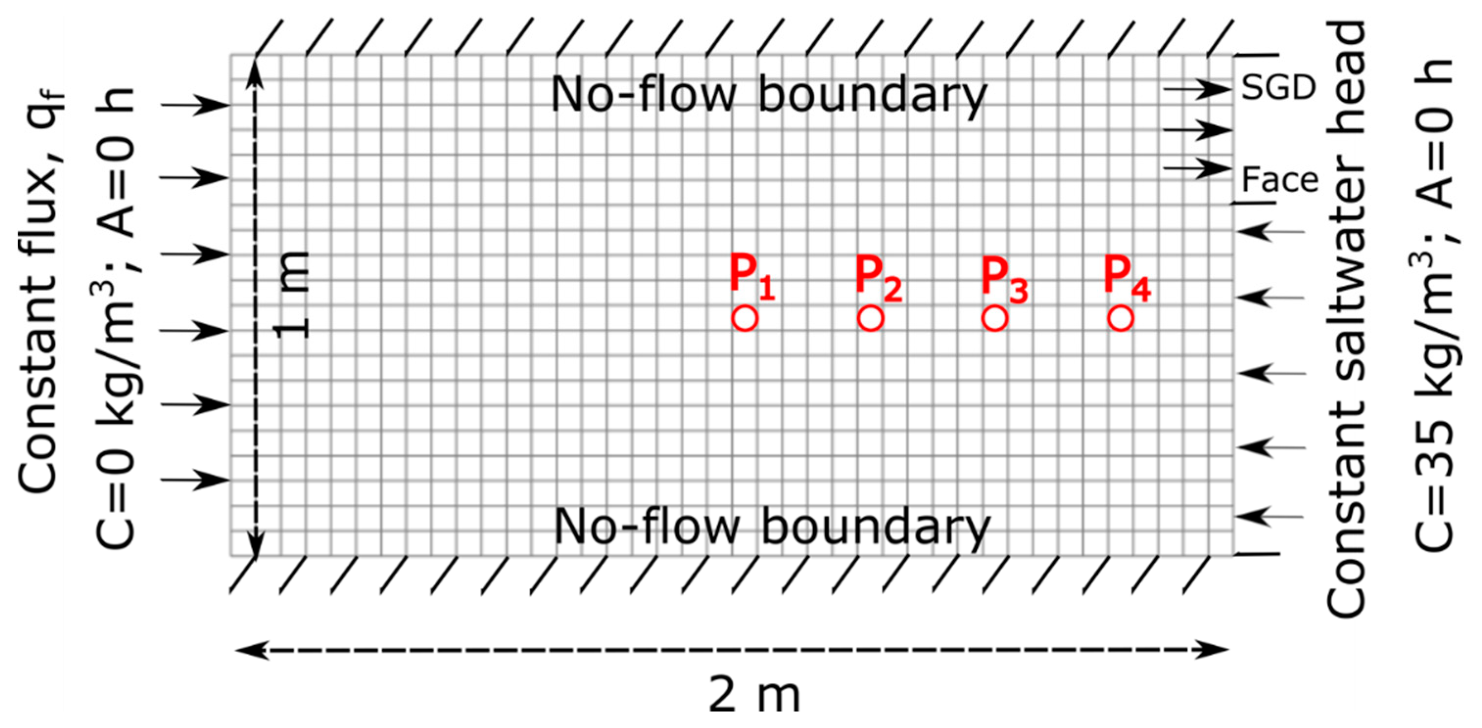
Some of the past controversial issues related to the suitability of the Henry problem for seawater intrusion problems were demystified more recently by Simpson and Clement [62], who suggested halving the landward freshwater recharge to increase the influence of the density-dependent effects. This modification is adopted in this work as shown in Figure 1, where prescribed boundary conditions are equally depicted. We assume that inflowing fresh and salt waters respectively from inland and sea boundaries have a zero age. Post et al. [64] argue that this might be a crude approximation owing to groundwater age stratification in subsurface aquifers. Nevertheless, because there is no formal way to assign these boundary conditions as have been noted by the same authors, we keep this hypothesis in the following. For more practical insights, we also consider a modified version of the Henry problem by including a pumping well at X = 100 m. We also consider the heterogeneous Henry problem suggested by Younes and Fahs [65]. Furthermore, the dispersive Henry problem [66] is equally considered in this work to elucidate the impact of enhanced freshwater-saltwater mixing mechanism on the vulnerability to seawater intrusion in a confined coastal aquifer. A uniform grid spacing at 5 cm was adopted for all simulations along the longitudinal and vertical dimensions. Details on further parameters are provided in

Table 1. Physical parameters used in the diffusive and dispersive variants of the Henry problem.

Parameter	Diffusive Henry Problem	Dispersive Henry Problem
Freshwater density ${\rho }_r$ (Kg·m−3)	1000	1000
Seawater density ${\rho }_s$ (Kg·m−3)	1025	1025
Seawater salinity $C_s$ (Kg·m−3)	35	35
Vertical hydraulic conductivity $K_z$ (m·s−1)	0.01	0.01
Anisotropy ratio ($K_z/K_x)$	1	0.66
Effective porosity $\varphi$	0.35	0.35
Molecular diffusion of salt $D_m$ (m2·s−1)	1.886 × 10−5	0
Longitudinal dispersivity ${\alpha }_L$ (m)	0	0.1
Transverse dispersivity ${\alpha }_T$ (m)	0	0.01
Freshwater flux qf (m·s−1)	3.3 × 10−5	3.3 × 10−5

.

4.1.1. The Diffusive Henry Problem

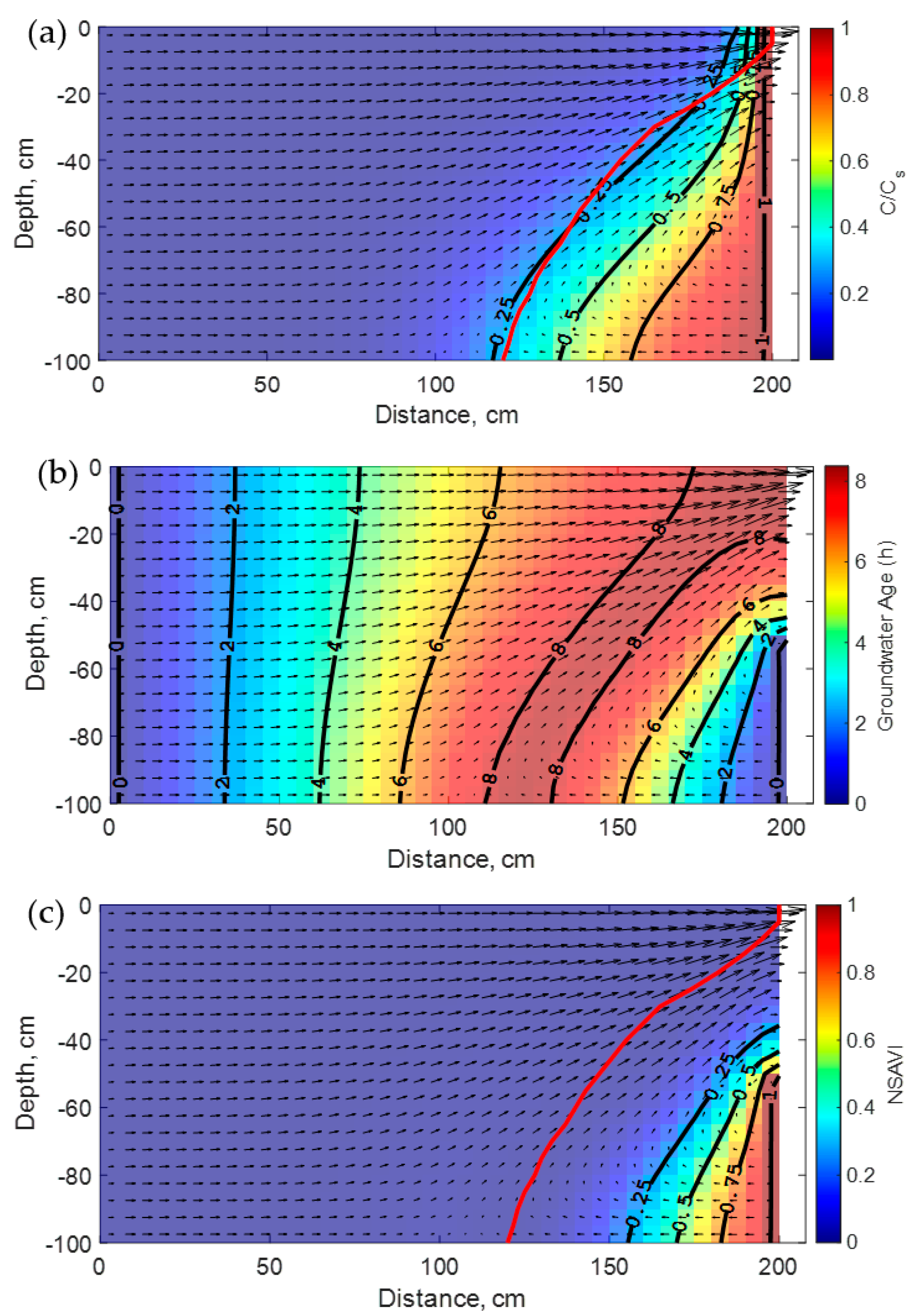
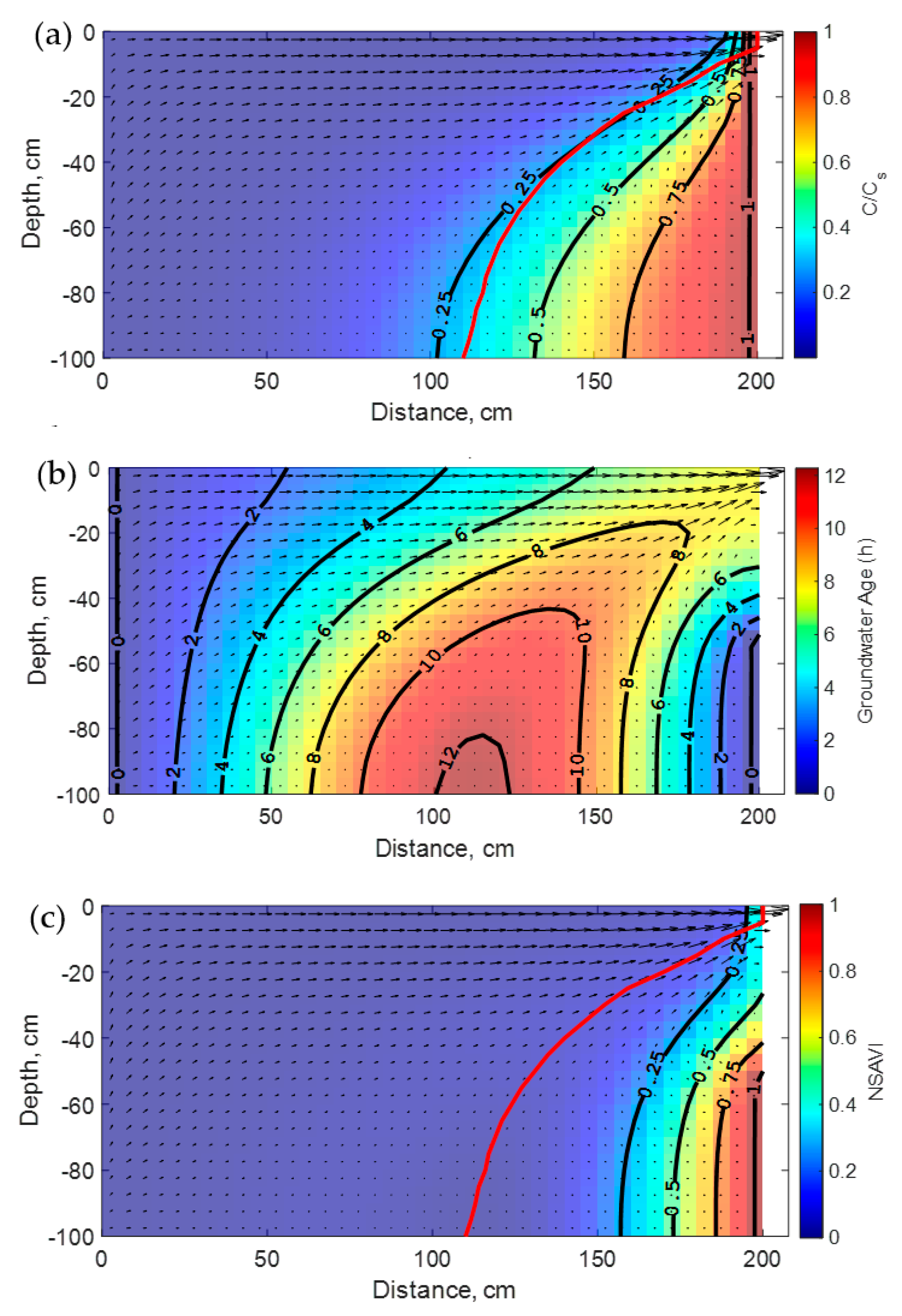
Figure 2a shows the results of the steady-state concentration isochlors profile for the Henry problem. In the same figure, the ridge of the groundwater age surface is also plotted. This also defines the spatial positions where the vulnerability to seawater intrusion equals zero (i.e., NSAVI(x) = 0). In the following, this will be identified as the zero-vulnerability line for a 2D space (or surface in three-dimensional space) and denoted thereafter by ZVL (or ZVS) depending on the space dimension. Owing to salt diffusion, a mixing zone develops at intermediate positions between the saltwater and freshwater zones. The landward transport of the salt is greater with the aquifer depth due to the density stratification. The same phenomenon is observed for the calculated vulnerability index as shown in Figure 2c where the vulnerability to SWI is higher as the aquifer depth increases close to the coast. However, the vulnerability plume is less extensive than that for the concentration distribution. This is because only some, but not all, cells in the mixing zone are located behind the ZVL.

The rationale for this observation is that the likelihood of seawater intrusion is different from the ultimate (i.e., at steady state) salinity that will be attained after a long time. This reflects the usefulness of the introduced approach as the time effects are implicitly incorporated in the definition of the NSAVI index (i.e., Equation (6)) while solving the groundwater age Equation (5).

The simulated direct age is shown in Figure 2b where the direct age gradient in the saltwater zone is higher than that in the freshwater zone. The highest direct groundwater age in the domain was 8.38 h, which occurs along the lower limit of the model at 120 m from the landward freshwater boundary. As noticed earlier [64], this is a velocity inflection point where horizontal freshwater and saltwater pathlines converge. Overall, the results presented in Figure 2b are in good agreement with previously published results [64], except that the calculated direct ages are higher herein because a lower freshwater flux value, q_f, was adopted.

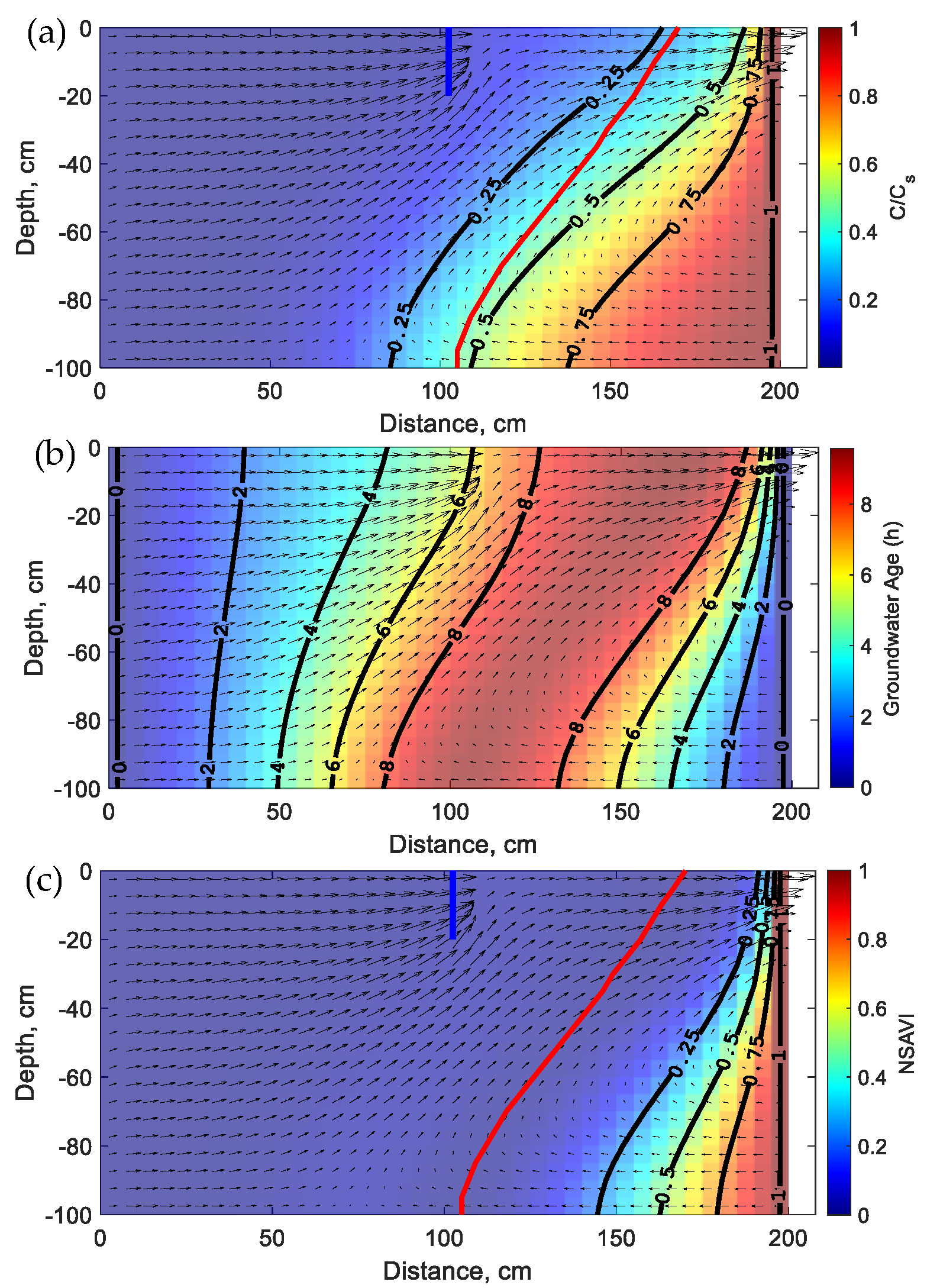
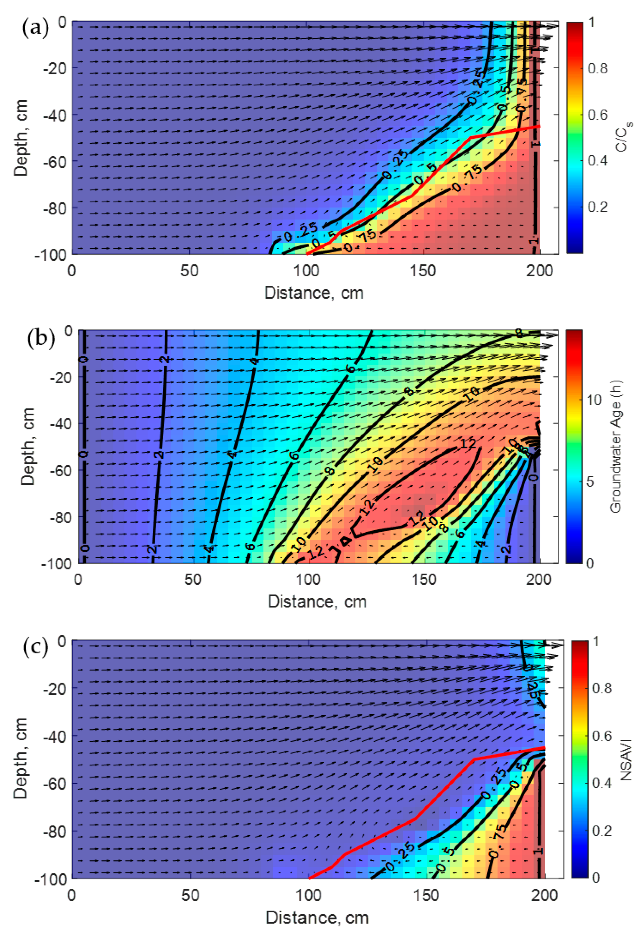
Results of the first modified Henry problem involving a 0.2 m partially penetrating well discharging groundwater with a rate of Q_p = 4 × 10⁻⁵ m³·s⁻¹ are visualized in Figure 3. Notably, the steady state concentration isochlors and vulnerability index plumes both advance landward because of pumping. Furthermore, their increased extension with the aquifer depth is noticed here again and is processed almost in the same way. 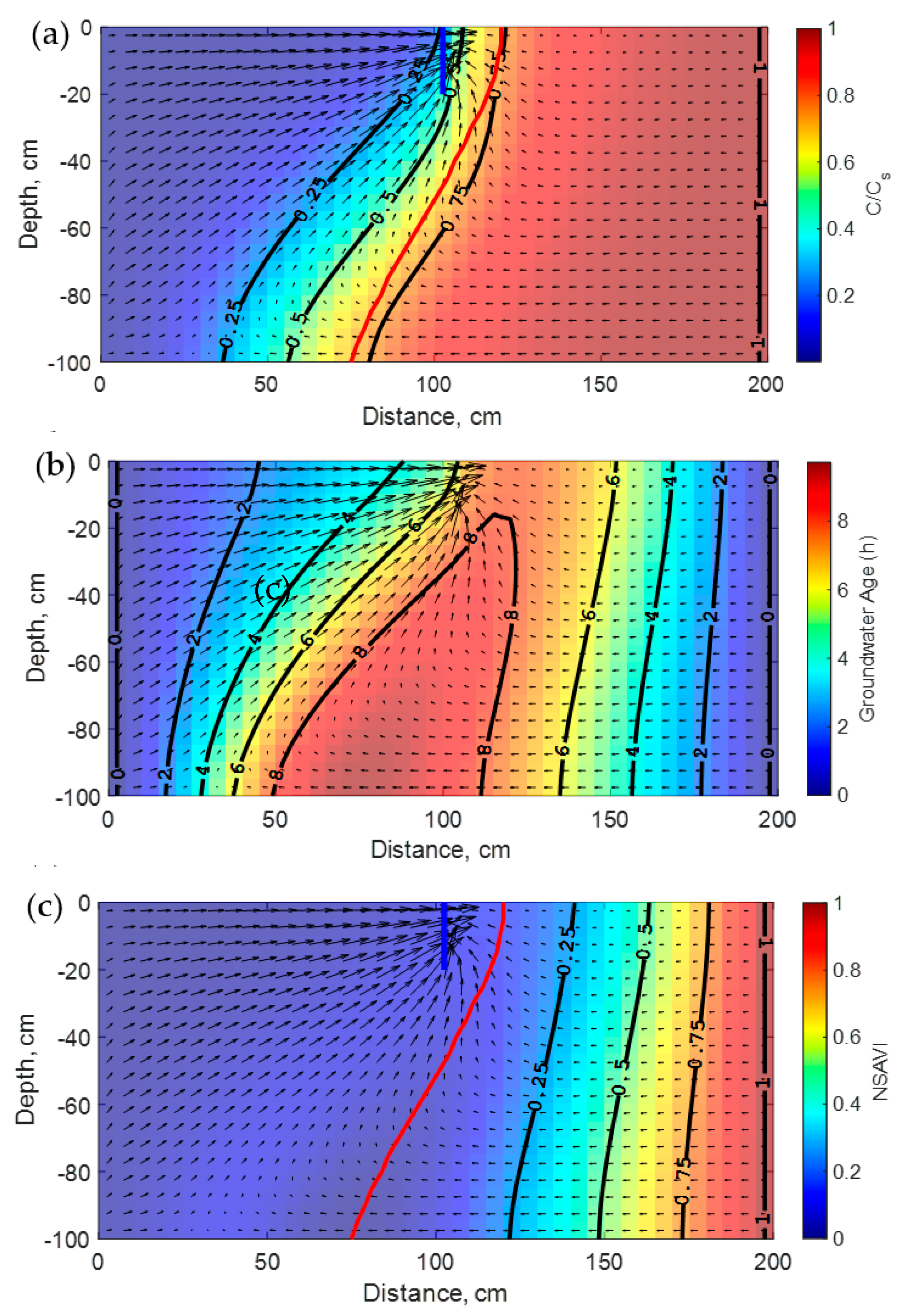However, as the pumping rate Q_p reaches 10⁻⁴ m³·s⁻¹ for the last test case as shown in Figure 4, saltwater upconing beneath the well becomes more pronounced implying significant vertical displacement of saltwater to the upper part of the aquifer. This is in agreement with the simulated steady state concentration isochlors and the vulnerability index profiles shown in Figure 3a,c, respectively. Hence, when the pumping rate in a well exceeds a critical value, yet to be determined, all the three-dimensional aquifer space separating this well to the coast becomes highly vulnerable to salinization. Although the selected example involves a confined aquifer, extrapolation to shallow unconfined aquifers suggests possible salinization of agricultural soils as the water table rises in winter periods and/or due to sea-level rise.

Figure 2a, Figure 3a and Figure 4a show the relative positions of the ZVL for each case. Notably, this line moves landward as the pumping rate increases. Most importantly, the ZVL is closer to the 25% isochlor at natural conditions, lies between 25% and 50% isochlors for the lower pumping rate, and becomes much close to the 75% isochlor for the highest pumping rate. This illustrates the fact that it will be hard in practice to select, a priori, a unique isochlor level as a metric to evaluate the vulnerability to SWI for contrasting anthropogenic conditions. Herein, as the pumping rate increases the ZVL will correspond to a higher isochlor level. This has important implications for practical coastal aquifers management as will be further discussed in the next section.

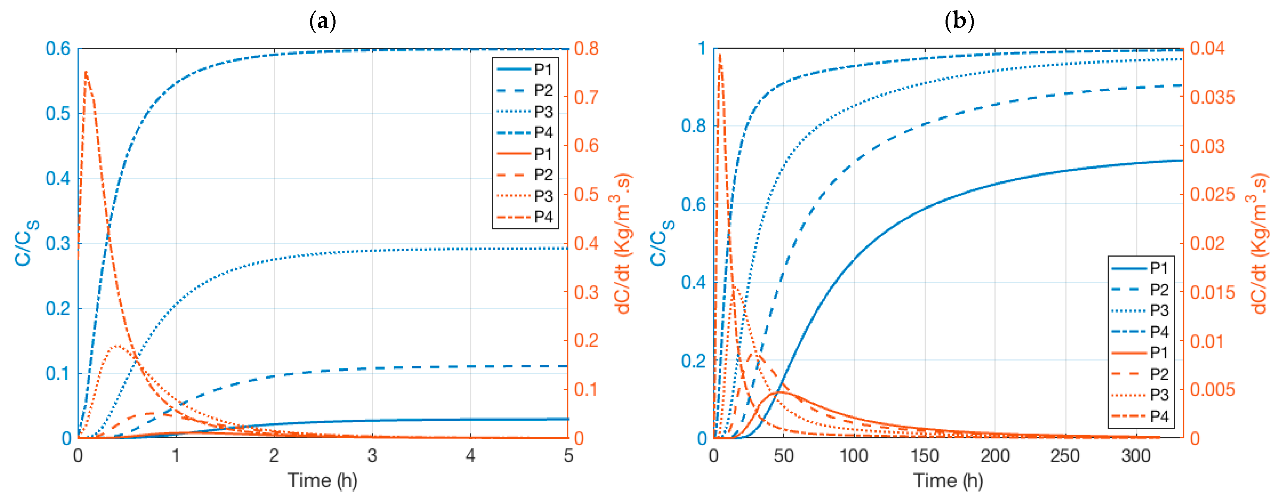
To further explain why the ZVL does not fit a fixed isochlor level for all variants of the diffusive Henry problem, we will consider the transience in the normalized concentrations (i.e., C/C_s) at the observation points P_1,…,4 shown in Figure 1. Hence, an additional two transient simulations of the VDFT problem are performed for the standard Henry problem and the variant with the highest pumping rate. Additionally, the salinization rate (i.e., dC/dt) time series are equally monitored at these locations. A constant time step size of 5 min was selected. However, as the chosen numerical solution scheme was the total variation diminishing scheme smaller internal time steps were automatically selected to enforce the numerical stability to satisfy the Courant number criterion [29].

Figure 5a shows the results for the diffusive Henry problem. The system attends an equilibrium state after few hours as concluded from the concentration time series at all observation points. This is not the case for the variant when pumping with the highest flow rate where the system attends an equilibrium state only after 316.67 h. Hence, salinization dynamics are almost two-orders of magnitude slower when comparing this variant with the standard Henry problem.

This behavior becomes even clearer when comparing the salinization rates in Figure 5a,b at each observation point. Salinization rates take the form of bell-shaped curves whose maxima are delayed as the distance from the sea boundary increases. When pumping occurs, the magnitude of the salinization rate becomes weaker, its maxima is delayed, and this function exhibits a long tailing indicating sustained salinization in time of the aquifer.

Hence, by increasing the pumping rate the ZVL will correspond to a higher isochlor level of the steady state salinity distribution because salinization kinetics become slower prior to attending an equilibrium state between freshwater and saltwater.

Pumping with the lower rate results in an extensive shift zone between the freshwater and saltwater regions containing the highest ages and an increase in the direct age pic (9.57 h; Figure 3b). However, the higher pumping rate induces a concavity of the high ages, a reversal of the age gradients in the freshwater and saltwater zones (i.e., high in freshwater and low in saltwater), and a further increase in the direct age pic (9.71 h; Figure 4b).

4.1.2. The Heterogeneous Diffusive Henry Problems

A heterogeneous Henry problem was introduced in [65] as a new suitable benchmark for the VDFT models for stratified domains where the permeability is variable with depth. It has been shown, in particular, that an exponentially decaying permeability with depth leads to more pronounced SWI manifested by a thicker mixing zone. Likewise, an exponential increase of the permeability produces a more retracted salinity wedge. The purpose of the following two test problems is, therefore, to reproduce this behavior and to demonstrate that the heterogeneity of the porous medium is another key factor to assessing the vulnerability of a coastal aquifer to SWI [35].

The standard Henry problem for a homogenous aquifer was slightly modified by allowing the intrinsic permeability, $k,$ of the porous medium to vary with depth following one of the relationships $k=k_b\exp \left[+\delta \left(1-z\right)\right]$ or $k=k{\prime }_b\exp \left[-\delta \left(1-z\right)\right]$, where k_b = 0.1604 × 10⁻⁹ m²; k′_b = 3.2216 × 10⁻⁹ m²; $\mp \delta$ is the decay/increase rate, and $z$ [L] is the aquifer depth. All the remaining physical and spatial discretization parameters remained identical as in the reference diffusive Henry problem. The effective diffusion coefficient was maintained as equal to that for the standard Henry problem (i.e., 1.886 × 10⁻⁵ m²·s⁻¹) for comparative purposes with the homogeneous simulations. Therefore, the results are expected not to be identical to those presented in [65] as they selected a smaller effective diffusion coefficient (i.e., 3.76 × 10⁻⁶ m²·s⁻¹) as suggested by other authors [67].

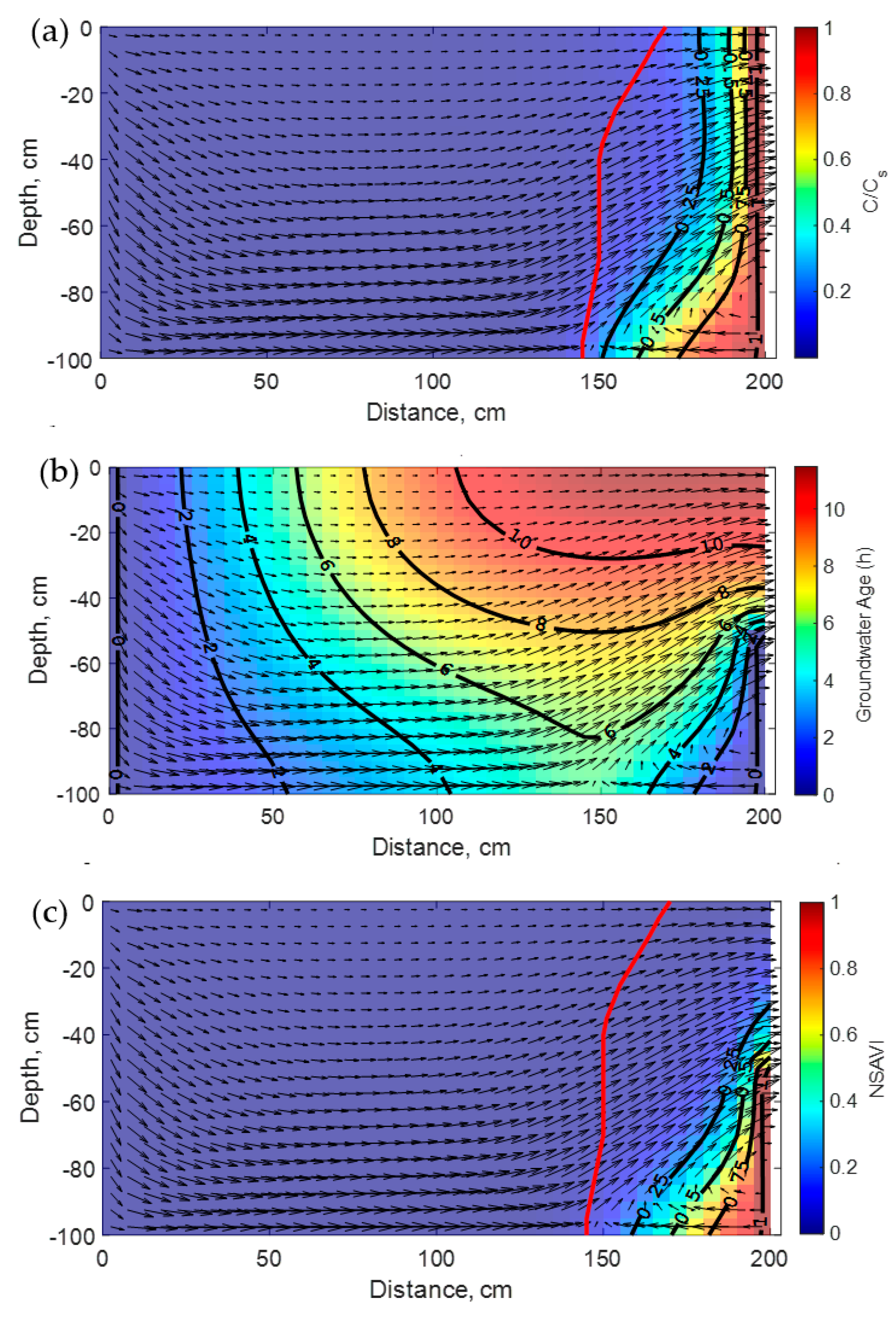
Figure 6 shows the simulated profiles of the steady state salinity, direct groundwater age, and the vulnerability index to SWI for the problem with a decaying permeability with depth. As indicated in [65], this configuration induces a further penetration of the salinity along the aquifer base as concluded when comparing Figure 2a and Figure 6a. As a result, the mixing zone is wider for this heterogeneous structure. Similarly, the obtained vulnerability index plume, shown in Figure 6c, is more diffuse and penetrates further inland than for the homogeneous case as depicted in Figure 2c. Conversely, increasing permeability with depth leads to higher groundwater velocities in the aquifer bottom pushing the salinity wedge seaward (Figure 7a).

Here again, the vulnerability to SWI (Figure 7c) is less important than in the standard Henry problem showing general consistency when the underlying processes. This is not the case for data-driven indexing methods such as GALDIT. Indeed, its direct application to the standard Henry problem and the two heterogeneous cases would give identical classes of the vulnerability irrespective of the heterogeneity structure. This is because $k_b$ and $k{\prime }_b$ were chosen such that the heterogeneous and the homogeneous cases have the same transmissivities. Hence, the six parameters needed for GALDIT would be identical for all three cases. Therefore, even basic examples lacking field scale complexities are providing further evidence for the limitations of the popular data-driven indexing techniques to produce reliable maps of the vulnerability to SWI.

Figure 6a and Figure 7a show also the ZVL delineating the spatial partition of the aquifer that will be likely threatened by saltwater intrusion. Similar to the homogeneous test cases, the ZVL’s for the two heterogeneous problems correspond to different isochlor levels demonstrating the unreliability of this metric alone for assessments of the vulnerability to SWI. For the decaying hydraulic conductivity case, the ZVL is close to the 25% isochlor while in the opposite case it fits a lower isochlor level.

Notably, the spatial direct groundwater age distributions for these two heterogeneous formations, as shown in Figure 6b and Figure 7b, exhibit concave and convex dome-like structures, respectively. For an exponentially decaying permeability with depth, the highest direct groundwater age in the domain was 12.27 h, occurs along the lower limit of the model at 110 m from the landward freshwater boundary. In the opposite case, the highest direct age was 11.48 h along the top model boundary at 30 m from the seashore.

4.1.3. The Dispersive Henry Problems

The dispersive Henry problem introduced in [66] is a variation of the Henry problem, which considers the hydrodynamic dispersion effect on the development of the mixing zone between freshwater and saltwater. Furthermore, unlike the standard Henry problem the anisotropy ratio (K_z/K_x) is smaller than for the ideal case (i.e., 1) as shown in Table 1.

The dispersive Henry problem shows a smaller transition zone while the toe of the saltwater wedge penetrates further inland as illustrated in Figure 8a. This is consistent with previous results [66]. Furthermore, the direct age distribution (Figure 8b) is similar to previously published results [64]. Indeed, the highest direct age is found along the lower limit of the model and decreases towards the upper right corner due to mixing with seawater having the lowest ages.

The vulnerability index for the dispersive Henry problem is slightly higher than for the diffusive variant, but only in the deepest zone near the seashore (Figure 8c). Hence, enhanced mixing of fresh and salt waters can non-uniformly increases the vulnerability to SWI within depth.

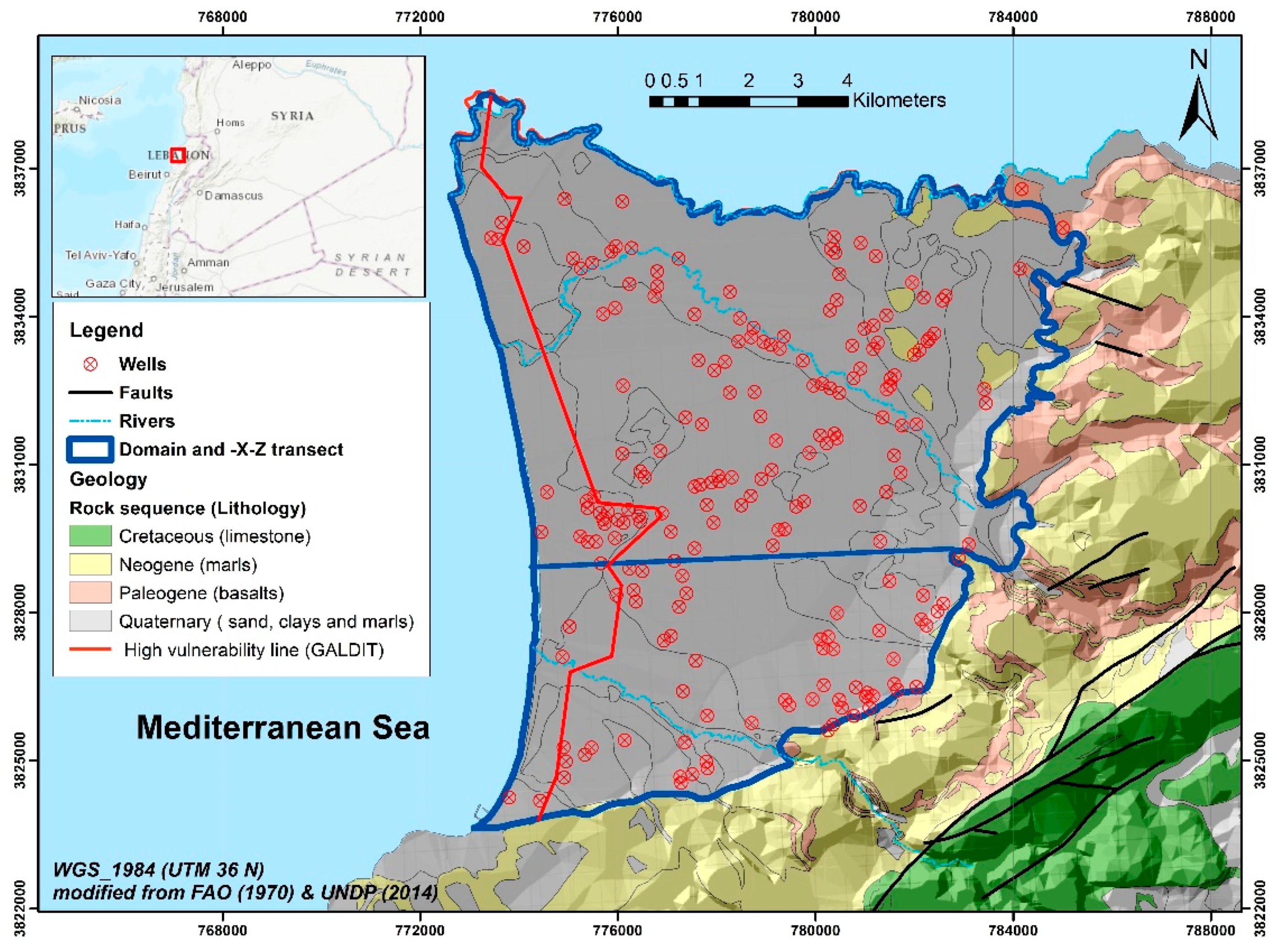
4.2. Example 2: The Akkar Coastal Aquifer (Lebanon)

The second demonstration problem involves the large Akkar coastal plain in Northern Lebanon. It is bounded by high mountains to the east and the Mediterranean Sea to the west as illustrated in Figure 9.

This plain has a rapid population growth exhibited by the massive migration of refugees from neighboring countries. Consequently, freshwater demands for potable and agricultural use have been steadily increasing. Because groundwater resources are the first source of freshwater supply in this area, the aquifer system is facing overexploitation and salinization risk. In the middle stretch of the plain, salinities have increased from an average value of 450 mg·L⁻¹ [68] to an average of 655 mg·L⁻¹ in 2013 [69]. Groundwater salinization is expected to extend further due to anticipated climate change impacts on water resources, especially in a semi-arid set up. Hence, in this work we investigate the vulnerability of this aquifer system to SWI. The performance of different management strategies is evaluated based on their distributed vulnerability indices.

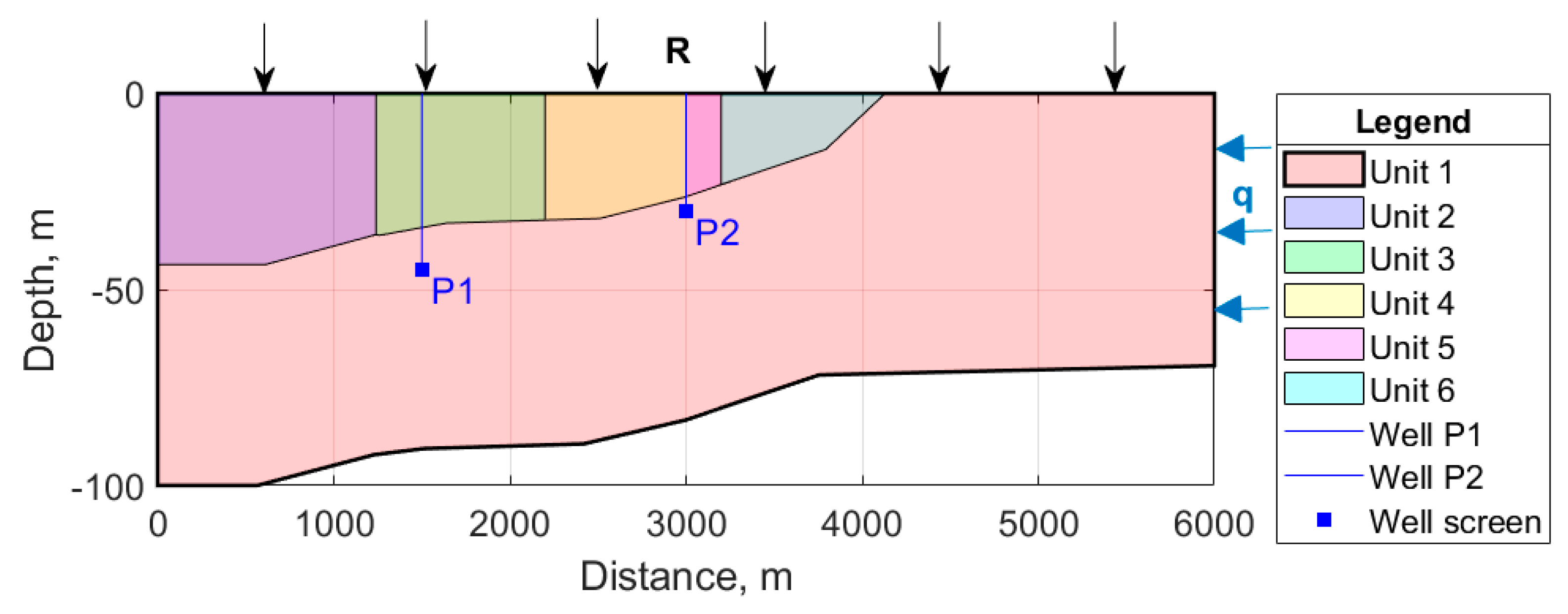
We consider the 2-D shore-perpendicular cross-section shown in Figure 9. Its lateral extension amounts to 6 km while the associated aquifer depth varies from 100 m close to the Sea to 69.5 m at the eastern boundary. Figure 10 shows the domain geometry as well as the six identified aquifer units whose hydraulic characteristics are summarized in

Table 2. Physical parameters used for the specific vulnerability assessments in the Akkar aquifer case study (Lebanon).

Parameter	Value
Freshwater density ${\rho }_r$ (Kg·m−3)	1000
Seawater density ${\rho }_s$ (Kg·m−3)	1025
Seawater salinity $C_s$ (Kg·m−3)	35
Dynamic viscosity $\mu$ (Pa.s)	1.002 × 10−3
	Unit 1: 1.01 × 10−12
	Unit 2: 1.01 × 10−12
Vertical permeability $k_z$ (m2)	Unit 3: 8.15 × 10−12
	Unit 4: 5.09 × 10−13
	Unit 5: 1.01 × 10−14
	Unit 6: 3.05 × 10−13
Anisotropy ratio ($K_z/K_x)$	0.1
Effective porosity $\varphi$	Units 2, 3, 4: 0.3
	Units 1, 5, 6: 0.2
Molecular diffusion of salt $D_m$ (m2·s−1)	10−9
Longitudinal dispersivity ${\alpha }_L$ (m)	50
Transverse dispersivity ${\alpha }_T$ (m)	5
Average recharge R (m·s−1)	3.86 × 10−7
Mountain-block recharge q (m·s−1)	6.40 × 10−9

.

The Mediterranean Sea on the western side is a Dirichlet boundary condition with a hydrostatic pressure distribution along the aquifer depth. Average groundwater recharge of 100 mm/month (i.e., 3.86 × 10⁻⁷ m·s⁻¹) is set as a fixed flux on the top surface boundary. At the landward boundary, we assume a constant mountain-block recharge flux estimated to 6.4 × 10⁻⁹ m·s⁻¹ from the east. For salt transport, we use a fixed salinity (i.e., 35 g·L⁻¹) boundary condition at the seaside. A null concentration is fixed landward and on the top boundaries representing freshwater influx. A zero age Dirichlet boundary condition was prescribed on the top, left and right boundaries. As shown in Figure 7, two pumping wells are considered for groundwater abstraction. The first pumping well, P1, is located near the sea (i.e., at 1500 m from the coast) at 45 m depth while the second pumping well, P2, is located further inland (i.e., at 3000 m from the coast) at 30 m depth. Actual pumping rates at P1 and P2 amount to 579.25 L·h⁻¹ and 604.25 L·h⁻¹, respectively.

The computational domain was discretized with a uniform structured finite-difference grid made from 600 columns and 20 layers. Thus, it is composed of 12,000 cells from which 9852 cells are set as active. The steady state solution of the coupled VDFT Equations (1)–(4) can be hard to obtain because, very often, of non-consistent initialization of the groundwater heads. This negatively affects the convergence behavior of the iteratively coupled scheme requiring either to sacrifice the numerical solution accuracy by selecting low convergence thresholds or to excessively increase the number of required outer iterations between the sparse flow and transport equation systems. This behavior was not observed, however, for the Henry problems, but has appeared during the simulations in this field case study. To overcome this problem, a steady state groundwater flow model using identical aquifer parameters, pumping rates, and flow boundary conditions was executed. Next, the obtained hydraulic heads initialize the steady state coupled VDFT model.

The actual distributed vulnerability index to SWI, NSAVI(x,z), was calculated with current natural and anthropogenic conditions in the Akkar coastal aquifer as shown in Figure 11a. It is shown that the aquifer is vulnerable to seawater intrusion as the ZVL extends up to 2740 m from the coast. Notably, the NSAVI gradient increases markedly seaward. As expected, the vulnerability increases also with the depth due to the density stratification as observed in many variants of the Henry problem. We iterate that this is not possible to achieve with the data-driven indexing methods. Indeed, GALDIT was implemented for the Akkar aquifer [70]. This study identified the highest vulnerability boundary between 1–1.5 km along the coast (Figure 9). As measured SWI goes beyond this highly vulnerable area, it was concluded that GALDIT is not accurate. Meanwhile, the measured salinity along the ZVL shown in Figure 11a is less than 500 mg·L⁻¹ confirming that it remarkably delimits the areas more affected by SWI.

A series of simulations were designed with management schemes involving (i) wells relocation, (ii) decreasing the well density (i.e., using only one pumping well in this case), and (iii) reducing the total pumping rate. Overall, we found that a combination of these three remediation actions was the most effective to aggressively decrease the specific vulnerability of the aquifer to SWI. Figure 11b shows the results obtained from concentrated pumping in a single well located midway between wells P1 and P2 along the distance and depth directions. In this scenario, the pumping rate was set to 946.8 L·h⁻¹, which amounts to 80% of the total pumping rate. The NSAVI isolines are drastically shifted seaward indicating a high potential for the aquifer remediation when using this management scenario. Indeed, the ZVL distance from the coast does not exceed 760 m leading to a reduced vulnerable area by almost one-third of the space that was initially under salinization threat.

This exemplifies how the introduced concepts could guide coastal aquifer management. These management tools are useful to adjust tradeoffs between negative environmental impacts, costs, feasibility, and public acceptance. This newly proposed management scenario is sub-optimal as only a trial-and-error procedure was used. However, when considering groundwater models with higher complexity in three-dimensional space considering many abstraction wells a simulation-optimization approach with the objective to push the ZVL seaward is a sounder alternative. This can be considered in future investigations, as the main objective in this paper is to demonstrate the relevance of the introduced concepts such as the NSAVI index and the related ZVL/ZVS for coastal aquifers management.

5. Discussions

Coastal aquifer management is the set of prevention and/or mitigation actions to fulfill short or long-term water demands according to given policies. Effective prevention of seawater intrusion needs an optimal monitoring network design. Different mitigation strategies have been identified to control seawater intrusion [15,71,72]. These can be divided among conventional, physical, and hydraulic barriers methods [72]. The conventional techniques aim at reducing/redistributing the pumping rates, relocating the pumping wells further inland, decreasing the wells density, or their cost-effective combination thereof. These are designed for short-term management actions before their replacement by barrier methods. While successful physical barrier projects have been reported in the literature, hydraulic positive and/or negative barrier techniques have attracted much more interest. Particularly, the low availability of freshwater resources in semi-arid and arid countries encourages the use of more economic sources of water (i.e., treated wastewater, harvested rainwater) for artificial recharge. As such, the proposed methods for management of SWI are ever increasing such that the optimal set to be selected becomes a challenge for each site-specific field site. The objective of this section is, therefore, to show how the introduced vulnerability mapping method can strive into sustainable management of coastal aquifers.

5.1. Implications of the Zero-Vulnerability Line/Surface on Coastal Aquifers Management

The zero-vulnerability line (or surface in three-dimension) is a new concept that is introduced in this paper for the first time to the authors’ knowledge. This interface simply delineates the spatial zone where there is a probability for seawater intrusion to occur depending on the system properties and applied stresses. In general, it will result from the intersection of many lines or surfaces dependent on the number of recharging/discharging boundary conditions, and the number of injection/pumping wells. The ZVL is an important communication tool to inform water resources managers, stakeholders, and decision-makers on the performance level of many management schemes. Owing to the relative simplicity in determining the ZVL, it will become a straightforward task to timely compare the effectiveness of many mitigation strategies even in three-dimensional aquifer space. In particular, the wells geographically located between the ZVL and the sea boundary could be ranked based on their vulnerability (the maximal NSAVI index along the well screens). Hence, simple schemes could be devised, and their effectiveness tested, to positively redistribute the pumping rates. When the ZVL is not too far from the coast, an important fraction of the total pumping rate could be reallocated to wells located landward of the ZVL. Moreover, we anticipate the technique to scale for field sites involving an important number of wells. As discussed in the previous section, the ZVL should not be confounded with the 50% isochlor, which highlights the unreliability of the latter as a metric for risk assessments in coastal aquifers. Notably, we believe that the ZVL is an effective educational and communication tool enabling to raise public awareness of the threats to coastal water resources resulting from global change impacts.

The ZVL and distributed NSAVI indices provide the building blocks towards a robust decision support system (DSS) simultaneously linked with subsurface earth models and GIS toolchains guiding water resources management in coastal areas. The availability of such information and communication technology (ICT) tool will be an important asset for real-time day-to-day active management and planning in a regulatory framework.

Owing to the inherent uncertainties in aquifer properties, groundwater recharge, future climate, and sea level rise future studies would advantageously consider a stochastic description of the ZVL. Thus, it will provide statistically based indicators of the potential risk to SWI and highlight the key-influencing parameters to improve their characterization.

5.2. Implications for Optimal Management of Coastal Aquifers

For sustainable management of coastal aquifers, a seawater intrusion simulation model is linked with an optimization algorithm to achieve a given management policy [28,29]. Management objectives are constrained by operational, environmental, and economical thresholds. These are, for instance, maximizing the wells pumping rates under the constraints of controlling the drawdowns and salinity below given thresholds. Nevertheless, single or multi-objective alternatives under different constraints may be devised for coastal aquifer management.

A linked simulation-optimization (S/O) procedure involves a very high computational cost limiting its widespread use in practice [72]. As such, many of the previous investigations have considered analytical solutions or the sharp interface approach as modeling components in the overall S/O loop [73,74]. Although other works have integrated the variable-density models within the S/O framework [75,76,77], a common limitation of these previous contributions, among others, is the extreme simplicity of the underlying seawater intrusion models. This has been necessary to avoid the bottlenecks related to computational time and non-convergence of the VDFT model at a given iteration jeopardizing the whole S/O process. This becomes more apparent with the community shift to evolutionary global optimization algorithms (i.e., genetic algorithms) which are more robust than the gradient descendent-based algorithms but requiring substantially more model evaluations.

As a remedy to these problems, a novel group of approaches has appeared using data-driven surrogate models constructed with the aid of machine learning algorithms [78,79,80]. Although some studies have reported impressive speedups for these S/O approaches, there remain many challenges in constructing and validating the surrogate models themselves [81,82]. Hence, the reported CPU time gains are offset by the hidden costs of the surrogate model training and validation.

We argue that a physical surrogate model serving the purpose of accelerating the S/O process for optimal coastal aquifer management might be a sound and more efficient alternative. An S/O approach embedding a process-based surrogate model for optimal groundwater remediation design converged in less than 2 h CPU time for a three-dimensional problem with 72,000 active cells [83]. As already highlighted in [72] no specific approaches have been reported based on model-driven surrogates for seawater intrusion problems. A multi-fidelity S/O technique that switches between VDFT and sharp interface approaches has been developed [84] although this requires building and integrating two different modeling approaches rising their incompatibility issue. A more feasible roadmap towards these next-generation surrogate models can consider the approach developed in this work. It would be not only feasible but a far computationally efficient alternative, to consider the vulnerability model given by Equations (1)–(6) as a surrogate to a transient VDFT model. Single and multi-objective formulations can be built by introducing novel optimization objectives such as minimizing the vulnerability to seawater intrusion at selected observation points. Moreover, other types of constraints could be equally introduced to formulate the optimization problem such as constraining the ZVL/ZVS to lie within a maximal distance from the coast. We expect this foreseeable approach to provide a fast, practical, and simpler means for the outreach to optimal management of coastal aquifers.

5.3. Monitoring Network Design and Implementation

The monitoring network design is essential for the efficient management of coastal aquifers. This method does not require continuous measurements of chloride/EC electrodes, whereas a common transient VDFT model does. This can lead to substantial decrease of costs in terms of monitoring network and continuous tracking of salinity because the mean groundwater age is used as an indirect indicator of salinity. The collected data such as groundwater levels and salinity can serve for the validation of the conceptual model of the study area through model calibration. The spatial distribution of the NSAVI index has the additional ability to guide the spatial location and the frequency of salinity sampling. Particularly, the three-dimensional vulnerability map would be useful to localize the depth of the wells at which to monitor the salinity. Moreover, in complex hydrogeological environments other hotspots may be identified suggesting new observation points. A quantitative S/O approach for the optimal design of the monitoring network [85] could be devised based on novel formulations as discussed in the previous subsection.

The approach presented in this paper is a straightforward one that integrates at the core of published computer packages for modeling SWI processes [49,50,51,86]. This will be a significant contribution to the groundwater modeling community allowing the approach reproducibility for other field studies. A future challenge for the wider applicability of this approach is to relax the assumption of steady state hydrological and anthropogenic stresses. While this is not an issue for long-term assessments, future thorough investigations are urged for more accurate short-term assessments of the vulnerability to SWI in highly dynamic systems such as in high permeability shallow alluvial aquifers.

Steady state VDFT models have not attracted special interest in the past. There emerges a need for a more efficient solution of the equation system 1–4 with novel computational techniques. For instance, the fully coupled solution of the long-term transient VDFT model had proven to be more efficient than a sequential solution procedure [87]. Moreover, novel matrix preconditioning techniques should be introduced in this framework to accelerate the convergence behavior of such a coupled system of equations. For instance, algebraic multigrid preconditioning [57] for the intermediate linear systems may prove more attractive than other standard preconditioned Krylov subspace methods [88]. Additional efforts are needed to compare this convergence behavior when considering the fixed-point or Anderson accelerated Picard [89] and Newton-Raphson iterations, respectively. Additionally, more robust techniques to recover from the convergence sensitivity to initial conditions are other areas of future research that would lead to routine vulnerability assessments to SWI in coastal aquifers using the introduced method in this work.

6. Conclusions

This paper presents a novel approach that unifies mapping the vulnerability to seawater intrusion in coastal aquifers with state-of-the-art practices for modeling variable-density groundwater flow and transport processes. It provides a solid conceptual framework for quantitative assessments of salinization risks and sustainable management of coastal water resources. This approach is a natural precursor to the transient variable-density flow and transport models. The following general conclusions can be drawn from this study:

• The normalized saltwater vulnerability index was obtained from steady state distributions of the normalized concentration and a restriction of the mean groundwater age to a mean saltwater age distribution. The approach provides a novel way to shift from the concentration space into a vulnerability assessment space to evaluate the threats to coastal aquifers.
• The vulnerability to seawater intrusion is higher as the aquifer depth increases in homogeneous and heterogeneous stratified aquifers. This behavior is not reproducible when using the data-driven indexing methods giving further evidence of their conceptual limitations.
• The zero-vulnerability line/surface delineates the coastal area for which there is a probability of seawater intrusion to occur. This novel concept has important implications for the optimal management of coastal aquifers and establishing related risk assessment methodologies.
• The zero-vulnerability line position differs from that of the 50% isochlor. As the strength of anthropogenic processes increase, the ZVL fits with increasing isochlor levels. Hence, the 50% isochlor is not a suitable metric to evaluate the vulnerability of coastal aquifers to seawater intrusion.
• The provided theoretical and field case study problems demonstrate the suitability of this approach to rank, compare and validate different scenarios for coastal water resources management.

Future directions towards expected numerical developments, application enhancements, and optimal management of coastal aquifers are given. Continued developments and research in this field will be of immense benefit to advance scientific understanding of saltwater intrusion and upconing threats to the most valuable resource for life on earth.