Assessment of Capsicum annuum L. Grown in Controlled and Semi-Controlled Environments Irrigated with Greywater Treated by Floating Wetland Systems

Abstract

Accumulation of trace elements, including heavy metals, were evaluated in soil and fruits of chilli plants (Capsicum annuum L.) grown under both laboratory-controlled and semi-controlled greenhouse location conditions. Chilli plant biomass growth in different development stages and fruit productivity were evaluated and compared with each other for the impact of growth boundary conditions and water quality effects. Treated synthetic greywaters by different operational design set-ups of floating treatment wetland systems were recycled for watering chillies in both locations. Effluents of each individual group of treatment set-up systems were labelled to feed sets of three replicates of chilli plants in both locations. Results revealed that the treated synthetic greywater (SGW) complied with thresholds for irrigation water, except for high concentrations (HC) of phosphates, total suspended soils, and some trace elements, such as cadmium. Chilli plants grew in both locations with different growth patterns in each development stage. First blooming and high counts of flowers were observed in the laboratory. Higher fruit production was noted for greenhouse plants: 2266 chilli fruits with a total weight of 16.824 kg with an expected market value of GBP 176.22 compared to 858 chilli fruits from the laboratory with a weight of 3.869 kg and an estimated price of GBP 17.61. However, trace element concentrations were detected in chilli fruits with the ranking order of occurrence as: Mg > Ca > Na > Fe > Zn > Al > Mn > Cu > Cd > Cr > Ni > B. The highest concentrations of accumulated Cd (3.82 mg/kg), Cu (0.56 mg/kg), and Na (0.56 mg/kg) were recorded in chilli fruits from the laboratory, while greater accumulations of Ca, Cd, Cu, Mn, and Ni with concentrations of 4.73, 1.30, 0.20, 0.21, and 0.24 mg/kg, respectively, were linked to fruits from the greenhouse. Trace elements in chilli plant soils followed the trend: Mg > Fe > Al > Cr > Mn > Cd > Cu > B. The accumulated concentrations in either chilli fruits or the soil were above the maximum permissible thresholds, indicating the need for water quality improvements.

1. Introduction

Some of the challenges facing water resource management include climate change phenomena, such as droughts linked to global warming. Anthropogenic activities have negatively affected natural resources, such as freshwater, in terms of its quality compared to international standards for safe usage [1,2]. Severe climate and environmental challenges have been predicted for Australia, the Middle East, North Africa, and the southern USA [3,4]. The world population in 2050 might hit 9.7 billion; this number could reach 11.0 billion by 2100 [5]. Furthermore, the population growth rate increase might also lead to mass migration. More than 67% of the world population could face water shortages by 2025 [6,7]. At least 50% will be under serious high water stress by 2030, as predicted by Scheierling et al. [8]. Water consumption is expected to increase by 40% in 2030 [9]. Consequently, more wastewater contaminated with organic, inorganic, and biological pollutants will be generated [1]. Discharging inadequately treated wastewater to watercourses could have serious effects on soil, aquatic ecosystems, and the public health [10,11]. Therefore, recycling treated wastewater for non-potable purposes is regarded as a feasible technique to mitigate water shortage. Thus, it is strongly recommended to treat wastewater before discharge or recycling [1].

Wastewater treatment and recycling are encouraged due to the rapid increase in the demand for water availability and the desire to protect the environment/public health. Agricultural irrigation is one of several options used to recycle processed wastewater for non-drinking usage [12]. Sustainability principles and concepts of organic farming systems have been introduced to industrial agriculture to improve environmental quality and human dietary needs [13]. Wastewater is one of the most important potential sources of recycled nutrients, reducing the need for fertilizers [14]. Irrigation within agriculture requires more than 70% of available water resources [15]. This proportion is likely to increase by around 14% in 2030, according to predictions by the Food and Agriculture Organization (FAO) [1].

In the 16th and 17th centuries, wastewater was already utilized as a water source for irrigation practices in Germany, Poland, and Scotland [16]. In the 20th century, governments, international originations, and agencies had issued legislation and standards to regulate the safe reuse of wastewater for irrigation purposes [4]. The intricacies associated with reusing or recycling wastewater for irrigation are linked to the community’s health and wider environmental risks, as discussed by Dalahmeh and Baresel [17]. Health risk concerns are associated with recycling wastewater for irrigation of plants of freshly edible roots, foliage, and fruits. Faecal pathogen contamination could spread in soil and adhere to plant tissues [18]. Safety, hygiene, aesthetics, environmental tolerance, as well as economic and technical feasibilities, are important assessment criteria [19].

In general, domestic wastewater has faecal constituents from toilet discharge, which is classified as black wastewater (BW), while wastewater generated from domestic activities is known as grey wastewater or greywater (GW). The majority of GW generated from laundry, showers, washing basins, dishwashers, and kitchens constitutes about 75% of the total domestic wastewater [20]. Therefore, recycling GW for agricultural irrigation has gained wide popularity, in terms of the low level of pathogens and nutrient contaminants [21,22].

There is a risk of accumulation of contaminants, such as metals in both soil and plant tissues [23,24], negatively effecting human and animal health [14]. Some plant species are able to grow in contaminated soils with elevated metal concentrations through hyper-accumulation processes [25]. Accumulated trace elements can significantly change soil enzymes, increase microorganism metabolic activities, and threaten bacterial functional diversity [26]. All metals in crops should be lower than the allowable concentration limits to reduce human health risks [27,28].

The allowable trace element concentrations in crops are stated according to their fresh weight and based on the daily intake. International regulations vary; e.g., India [29], China [30], European Union [31], United States Environmental Protection Agency [11], and the Food and Agriculture Organization (FAO)/World Health Organization (WHO) of the United Nations [27,32]. Leafy and root vegetables represent higher health risks than fruits, since metals accumulate in roots and leaves of crops rather than their fruits or nutrient storage organs [33,34]. Some vegetable cultivars have a high ability to accumulate nutrients compared to other species [35]. However, other studies have indicated an accumulation of arsenic (As), cadmium (Cd), lead (Pb), and chromium (Cr) in fruits, such as chillies [36,37]. Trace element levels in vegetable biomass vary, because of differences in application of contaminated water for irrigation (wastewater), contaminated soil (sewage sludge), fertilizer, pesticides, contaminated organic waste manure, industrial by-products, and inadequate water management strategies [28]. Some heavy metals are classified as biologically beneficial elements including cobalt (Co), copper (Cu), nickel (Ni), and zinc (Zn), which are required to build cellular and human organ tissues. However, elevated levels cause toxicity [34,38,39].

Practical and scientific efforts crucially focus on efficient and sustainable non-conventional wastewater treatment methods, which are low in capital expenditure, operation, and maintenance costs, and are environmentally friendly, such as wetland systems. Constructed wetlands (CW) are recognised as vital engineering solutions for conservation of water resources, not only for arid and semi-arid regions, but also internationally [40,41]. Wetland systems as ecological treatment technology for wastewater enhance sustainable water resources and produce effluents that could be used for recycling purposes by the agricultural irrigation industry [42]. Constructed wetlands remove pollutants by biological, chemical, and physical processes with moderate capital expenditures, consuming low energy, and requiring low efforts for maintenance and operation [43,44,45]. To avoid claiming too much expensive land for CW, the engineering innovation free water surface constructed wetland (FWS-CW) has led to the introduction of floating treatment wetlands (FTW) [46]. These floating systems are innovative ecological approaches to control water quality from point and non-point source pollution [47]. Aquatic macrophytes are cultivated hydroponically on water surfaces by artificial floating mats. Large surface areas within the water column are provided for microorganisms. Biofilms are attached to macrophyte roots and rhizomes, which are not grown in substrate [48]. Free-floating plants usually have high efficiencies in uptake of heavy metals from water compared to submerged and emergent macrophytes, due to their high growth rate and specific morphology [49].

The main objective of this study is to assess the suitability of processed greywater by FTW to be recycled for the irrigation of chilli plants grown in two different environmental conditions (laboratory and greenhouse). The corresponding objectives linked to achieve the main target are to assess (a) the effect of the environmental boundary conditions on plant growth and fruit productivity; (b) the economic benefit of different operational design variables of the FTW for fruit productivity; (c) the accumulated trace elements in soil; and (d) the accumulated trace elements in chilli fruits.

2. Materials and Methods

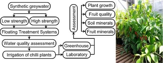
2.1. Operational Design of Floating Treatment Wetlands

Greywater was created artificially under laboratory-controlled conditions using analytical-grade chemicals obtained from Fisher Scientific Co., Ltd., Bishop Meadow Road, Loughborough, UK [50]. Two chemical formulas of different recipes were selected to represent synthetic greywater (SGW) in low and high pollutant concentrations, LC-SGW and HC-SGW, respectively, see Supplementary Material (Table S1). Concentrated stock solutions for both recipes were prepared separately, and diluted later as one part to 100 parts of tap water at each experimental treatment cycle.

The experimental treatment systems comprised 72 mesocosm-scale plastic buckets of 14-L with a depth of 0.3 m and a diameter of 0.25 m, filled with 10 L of SGW, which was operated to resemble natural floating reed islands [51]. The experiment was operated under authentic weather conditions on an open flat roof of the Newton Building, The University of Salford, Manchester, UK. Bare-rooted Phragmites australis (Cav.) Trin. ex Steud. (Common reed) plants provided by VESI Environmental, Ltd. (Little Island, Co. Cork, Ireland) were utilised to float on the mesocosm water surface [52].

Mine water sludge (ochre) collected from North Rochdale at the Deerplay Coal Mine (OL13 8RD), UK, was included in some of the treatment systems as adsorbent substances to enhance the performance of FTW. Three parts of Ordinary Portland Cement (OPC) were added to seven parts of raw ochre sludge to create cement–ochre pellets [53].

The water quality tests commenced on 1 September 2014, and ended on 1 November 2016. However, assessments only started on 1 November 2014, to allow two months for biofilm growth (September and October, 2014).

There were four operational design variables for the FTW systems: strength of greywater pollutants (LC-SGW and HC-SGW), hydraulic retention time (HRT; 2 and 7 days), presence or absence of macrophytes (Phragmites australis), and presence or absence of cement–ochre pellets [51]. The general experimental set-up of FTW systems consisted of two groups of mesocosms treating SGW for 2 and 7 days of HRT. The experiment had three groups of mesocosms: first group for treatment of HC-SGW (T1, T2, T3, and T4 for 2 days HRT; T9, T10, T11, and T12 for 7 days HRT); the second group for LC-SGW (T5, T6, T7, and T8 for 2 days HRT; T13, T14, T15, and T16 for 7 days HRT); and the third group for tap water (TW), which was considered for control purposes (C1 and C2 for 2 days HRT; C3 and C4 for 7 days HRT). Each set in the first and second group had four replicates, except for the third set of controls, which had two replicates of mesocosms. The treatment systems of T1, T2, T5, T6, T9, T10, T13, T14, C1, and C3 contained floating Phragmites australis, while 300 g of cement–ochre pellets were used to treat 10 L of SGW in the mesocosms T2, T4, T6, T8, T10, T12, T14, and T16. Afterward, a combination of Phragmites australis and ochre pellets was used in the systems T2, T6, T10, and T13, while systems of only SGW were linked to mesocosms T3, T7, T11, and T15 (

Table 1. Operational parameters in the experimental set-up supporting the irrigation of chilli plant Capsicum annuum L. with treated greywater by different designs of floating wetland systems [51].

Treatment System	HRT		SGW		TW	Vegetation		Cement–Ochre		Plant Receiving the Effluent
	2-Day	7-Day	HC	LC		With	Without	With	Without
T1	♦		♦			♦			♦	P1
T2	♦		♦			♦		♦		P2
T3	♦		♦				♦		♦	P3
T4	♦		♦				♦	♦		P4
T5	♦			♦		♦			♦	P5
T6	♦			♦		♦		♦		P6
T7	♦			♦			♦		♦	P7
T8	♦			♦			♦	♦		P8
T9		♦	♦			♦			♦	P9
T10		♦	♦			♦		♦		P10
T11		♦	♦				♦		♦	P11
T12		♦	♦				♦	♦		P12
T13		♦		♦		♦			♦	P13
T14		♦		♦		♦		♦		P14
T15		♦		♦			♦		♦	P15
T16		♦		♦			♦	♦		P16
C1	♦				♦	♦			♦	P1c
C2	♦				♦		♦		♦	P2c
C3		♦			♦	♦			♦	P3c
C4		♦			♦		♦		♦	P4c

Note: ♦, selection mark; T1–T16, treatment systems with four replicates; C1–C4, control treatment systems with two replicates; HRT, hydraulic retention time; SGW, synthetic greywater; HC, high pollutant concentration of SGW; LC, low pollutant concentration of SGW; TW, tap water; and P1–P4c, chilli plant with three replicates.

). Treated SGW (effluents) was replaced by freshly created SGW (influents) after the specific HRT, without disturbance of the biofilm that was attached to the macrophyte roots/rhizomes and on the vessel interior walls [51].

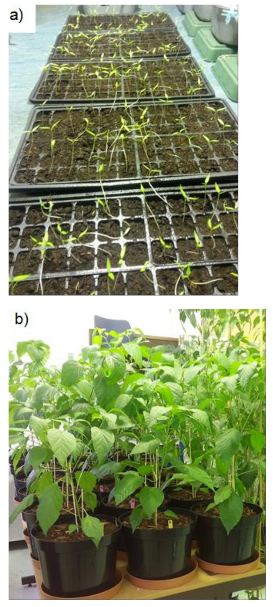
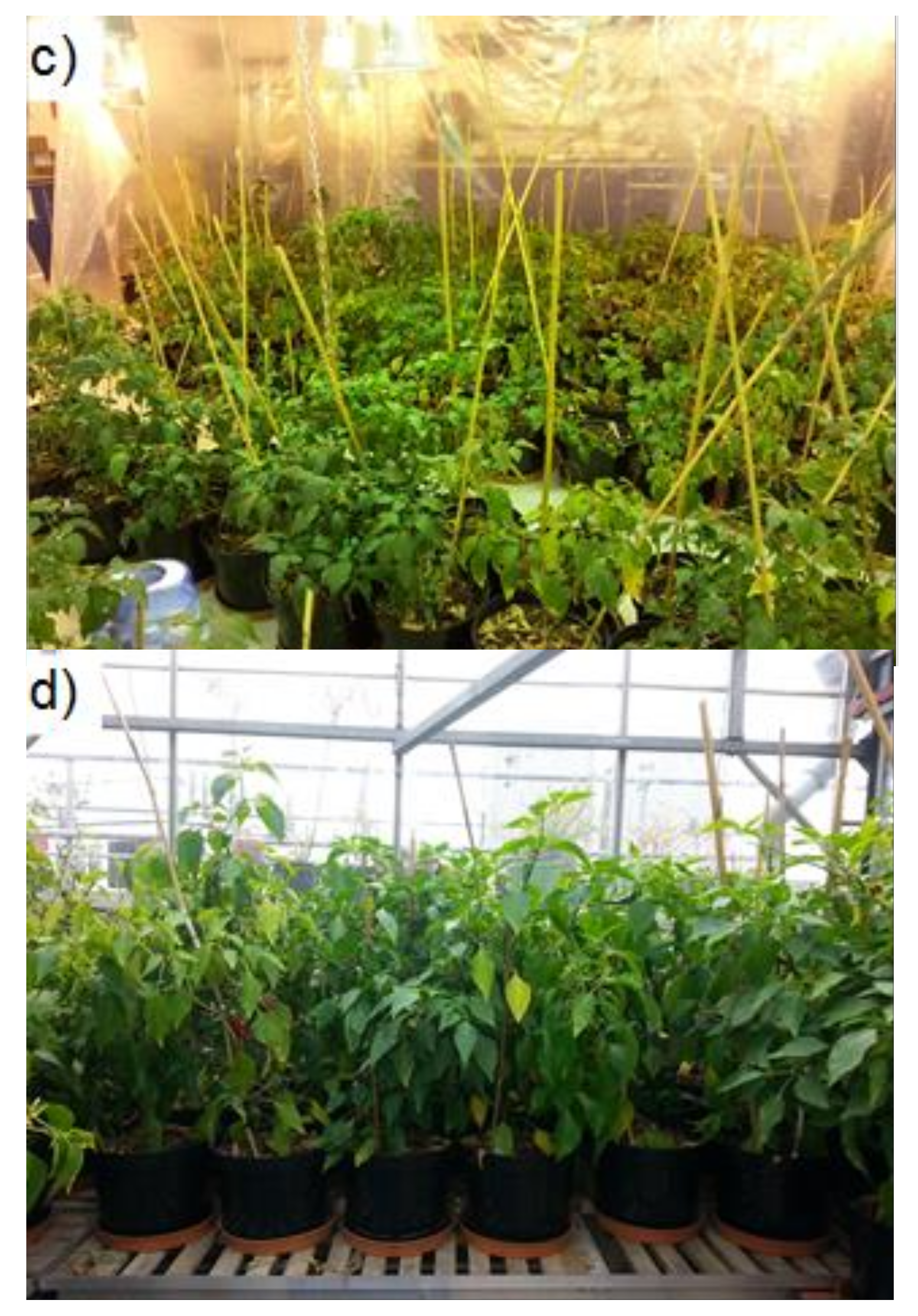
2.2. Material Selection and Chilli Planting Processes

The effluent from each FTW type was designated to be recycled for watering one set of chilli plants, which consisted of the three replicates a, b, and c (Table 1). Planting media, bark, and chilli pepper seeds “Verve Brand” (www.diy.com; accessed on 9 August 2021) were purchased from a local B&Q plc warehouse in Salford, Greater Manchester, UK (unless mentioned otherwise). Multipurpose peat-based compost soil (product code: 03717644) was selected as a planting media [54]. The dry composition of raw compost (before planting) comprised organic matter (89%), total phosphorus (368 mg/kg), total nitrogen (999 mg/kg), potassium (2776 mg/kg), and zinc (26.59 mg/kg) [4]. Small chipped bark (product code: 5397007188110) of mixed wood was applied on the top of the compost soil to maintain moisture and insulate the soil within the pots.

According to the supplier, the compost soil contained 42% of non-peat compost, which was a mixture of composted green waste and spent brewery grains. While the majority (58%) was sustainably sourced material in terms of ecological, archaeological, and conservation criteria. This product contained green compost, wood fibre, coir (natural fibre extracted from the husk (outer shell of coconuts) and oyster shells), Sphagnum moss peat, and unspecified amounts of composted bark, vermiculture, perlite, loam, charcoal, sand, grit, wetting agent (to retain moisture better; 200–400 mL/m³), essential nutrients, and trace minerals. The fertilizer and dolomitic limestone content were up to 3 kg/m³ and up to 7 kg/m³, respectively. However, the exact combination of all ingredients is confidential for commercial purposes. Therefore, the compost soil had a variable content with a complex structure and a bulk density between 200 and 450 g/L. A low bulk density and a high organic content proportion of compost provides a substrate with a high total porosity, stable soil structure, good hydraulic conductivity, as well as a high water retention time. A good compost water holding potential and water retention capacity is linked to high soil porosity. In addition, the authors reduced water evaporation and increased the moisture content of the compost by covering the top compost layer with small-chipped bark [3].

Chilli pepper seeds (De Cayenne; Capsicum annuum L. Longum Group; product code: 03623879) were purchased on 19 November 2014, to assess their growth when irrigated with artificial greywater pre-treated by differed designs of floating wetland systems. On 21 November 2014, about 180 single seeds were sown into a propagator, which was semi-filled with compost. One or two seeds were put in each propagated cell and covered with a thin compost soil layer of 6 mm thickness. On 19 December 2014, all propagators were protected by transparent covers to maintain the moisture content of the soil. The plants were kept in a dark incubation room at 20.8 °C until the seeds germinated. The recommended range by the supplier was 18–25 °C. After seed germination, all propagators were relocated to a laboratory fitted with the grow lights OSRAM HQL (MBF-U), which were high-pressure mercury lamps (400 W; Base E40) purchased from OSRAM (North Industrial Road, Foshan, Guangdong, China). The lamps were linked to a H4000 Gear Unit provided by Philips (London Road, Croydon, CR9 3QR).

The germination time was between 5 and 14 days, while the sowing to cropping period was 18 weeks [54]. All lights were electrically controlled by timers to simulate both sunrise and sunset times (http://www.timeanddate.com; accessed on 9 August 2021). The temperature near to the plants was around 19.3 to 26.3 °C with an average of 24.2 °C. On 13 February, 2015, true stems and more than two leaves were observed for almost germinated seedlings (Figure 1a). The strongest 150 chilli pepper plants were transplanted individually in round plastic pots of 10 litres (220 mm height, 220 mm bottom diameter, and 285 mm top diameter) purchased from ScotPlants Direct (Hedgehogs Nursery Ltd., Crompton Road, Glenrothes, Scotland, UK). Seedlings were transplanted in pots filled with moist multipurpose compost soil up to a height of 175 mm and topped-up with a layer of small chip bark of 25 mm thickness, while the remaining height of the pot (20 mm) was left as free space for irrigation water and litter. Another 10 chilli plants were also prepared in the same manner to serve as spare plants; i.e., substitutes (Figure 1b). Weak stems were initially supported by small bamboo sticks, and all plants were subjected to the same laboratory-controlled conditions.

The healthiest 120 chilli plants were selected from the grown plants to be part of the experiment: 60 plants were left in the laboratory (Figure 1c), while the remaining 60 plants were transported to the greenhouse (Figure 1d). On 20 March 2015, treated greywater (effluents of the FTW) was applied for watering chilli plants in the laboratory and greenhouse simultaneously. Since, the FTW system designs consisted of 20 mesocosm sets, effluent from each mesocosm set irrigated 20 chilli plant sets of three replicates in both the laboratory and greenhouse (Table 1).

2.3. Growth Environment Monitoring and Recording

Laboratory and greenhouse environmental boundary conditions, such as light intensity, relative humidity, and temperature, were monitored. The effect of these two different growing environments on chilli plant growth and fruit quality was also investigated, and comparisons between them were made to highlight any possible significant differences.

In both the laboratory and greenhouse, light intensity measurements were indicated by the LUX meter ATP-DT-1300 for the measurement range 200 l× to 50,000 l× (TIMSTAR, Road Three, Winsford Industrial Estate, Winsford, Cheshire, UK). The temperature and relative humidity were measured using a thermometer hygrometer station obtained from wetterladen24.de (JM Handelspunkt, Gschwend, Germany).

In the laboratory, room temperature was controlled using electric heaters (Rhino H029400 TQ3 2.8 kW Thermo Quartz Infrared Heater 230 V) provided by Express Tools Ltd. (Alton Road, Bournemouth, UK). The humidity was regulated by operating humidifiers (Challenge 3.0 L Ultrasonic Humidifier; Argos, Avebury Boulevard, Central Milton Keynes, England, UK). The provided lights were set on electric-powered timers to mimic sunshine hours.

2.4. Justification of Chilli Plant Selection

Chilli pepper plants (De Cayenne; C. annuum (Linnaeus) Longum Group) grown with recycled treated greywater were selected due for public health and safety, environmental, and economic reasons. Chilli fruits usually hang far above (at least 45 cm) the soil surface; therefore, they are subjected less to microbial contamination in comparison to plants with edible parts, such as salad or strawberries grown in potential contact with the soil [55]. According to the supplier (B&Q plc)—chilli has slender and hot fruits and can be grown easily in pots at various locations. The environmental growth conditions of chilli plants are comparable to those of warm geographical areas, but they can also be grown in British greenhouses [55,56]. Chilli prefers moist and loamy nutrient-rich soil with a pH range between 7.0 and 8.5 [54]. In addition, chillies are mostly perennial in tropical and sub-tropical regions (for at least three years). Commercial growing of chillies is easy, popular, and cost-effective. The plants are easy to obtain, have a high nutritional value, and are perfect for general cooking. The chilli growth time from sowing to cropping is only around 18 weeks. The germination time is between 5 and 14 days. Approximately 100 days are required for the plants to reach maturity.

2.5. Water Quality, Soil, and Chilli Fruit Analysis

Water samples were obtained from the effluents of FTW after specific HRT of treatment to assess water quality according to the standard methods for the examination of water and wastewater [57], unless stated otherwise (

Table 2. Influent and effluent (irrigation water) properties of synthetic greywater (SGW) treated by floating treatment wetland systems (FTW).

Parameter [57]	Unit	Influent	2-Day HRT (HC-SGW Effluent)				Influent	2-Day HRT (LC-SGW Effluent)
		HC-SGW	T1	T2	T3	T4	LC-SGW	T5	T6	T7	T8
pH	–	8.4 ± 1.61	7.4 ± 1.09	8.8 ± 1.69	7.8 ± 1.37	8.7 ± 1.73	6.9 ± 0.48	7.0 ± 0.71	10.5 ± 1.12	7.5 ± 0.70	10.6 ± 0.99
Redox potential	mV	−36.6 ± 74.22	8.1 ± 52.68	−54.8 ± 83.66	−3.0 ± 62.95	−49.9 ± 83.61	34.1 ± 21.23	27.5 ± 32.18	−137.4 ± 54.91	4.2 ± 30.40	−143.5 ± 51.01
Turbidity	NTU	188.9 ± 47.22	175.9 ± 59.61	223.8 ± 97.40	192.1 ± 50.87	191.3 ± 84.41	22.9 ± 7.14	28.2 ± 37.09	39.2 ± 45.10	20.2 ± 14.20	35.6 ± 18.11
Total suspended solids	mg/L	317.0 ± 58.35	302.9 ± 75.19	422.5 ± 152.77	321.8 ± 56.68	337.4 ± 109.45	39.9 ± 15.94	41.7 ± 43.57	62.0 ± 49.93	30.0 ± 12.12	66.2 ± 36.63
Electronic conductivity	µS/cm	988.5 ± 196.09	987.4 ± 107.25	1174.5 ± 282.81	965.2 ± 106.68	1178.4 ± 264.41	164.6 ± 63.24	145.9 ± 30.41	371.5 ± 260.12	138.5 ± 23.26	344.5 ± 287.03
Dissolved oxygen	mg/L	10.5 ± 1.39	9.0 ± 1.03	9.0 ± 1.24	10.2 ± 0.73	10.0 ± 0.52	10.4 ± 1.24	9.3 ± 1.08	8.8 ± 0.87	10.5 ± 0.82	10.1 ± 0.73
Colour	Pa/Co	1587.8 ± 379.89	1525.6 ± 411.54	2150.8 ± 864.04	1527.6 ± 326.28	1935.6 ± 702.18	214.5 ± 64.07	183.7 ± 74.89	308.2 ± 134.65	164.5 ± 40.93	331.7 ± 119.34
Temperature	°C	16.9 ± 5.40	17.1 ± 4.92	17.4 ± 4.87	17.1 ± 4.75	17.2 ± 4.73	17.7 ± 4.58	17.0 ± 4.84	16.6 ± 4.55	16.0 ± 4.59	16.3 ± 4.24
Biochemical oxygen demand	mg/L	34.7 ± 12.99	17.7 ± 6.40	11.1 ± 5.89	14.7 ± 7.78	11.7 ± 7.71	17.6 ± 8.00	9.9 ± 5.49	5.4 ± 4.36	5.6 ± 3.60	4.4 ± 5.13
Chemical oxygen demand	mg/L	129.2 ± 34.68	96.3 ± 32.01	109.2 ± 24.38	106.6 ± 22.68	100.3 ± 21.08	28.9 ± 14.47	32.4 ± 14.55	29.6 ± 16.67	26.8 ± 6.18	24.0 ± 4.99
Ammonia–nitrogen	mg/L	0.4 ± 0.19	0.4 ± 0.21	0.4 ± 0.13	0.4 ± 0.16	0.4 ± 0.09	0.2 ± 0.22	0.1 ± 0.07	0.2 ± 0.14	0.09 ± 0.05	0.1 ± 0.04
Nitrate–nitrogen	mg/L	8.9 ± 6.38	14.1 ± 6.40	14.3 ± 5.02	9.4 ± 4.67	12.9 ± 7.03	1.3 ± 1.21	1.7 ± 1.13	0.4 ± 0.33	1.2 ± 0.71	0.6 ± 0.54
Ortho-phosphate–phosphorus	mg/L	59.1 ± 14.16	52.0 ± 14.87	21.1 ± 5.81	46.2 ± 10.74	19.5 ± 4.98	8.4 ± 4.36	7.6 ± 3.90	3.2 ± 1.16	7.0 ± 3.89	3.9 ± 1.25
Element [58,59]
Aluminium (Al)	mg/L	2.13 ± 0.869	1.54 ± 1.479	2.02 ± 1.624	2.41 ± 1.016	2.98 ± 2.087	0.52 ± 0.528	0.08 ± 0.054	1.07 ± 0.874	0.34 ± 0.180	0.76 ± 0.347
Boron (B)	mg/L	0.57 ± 0.068	0.53 ± 0.086	0.41 ± 0.079	0.54 ± 0.060	0.50 ± 0.078	0.14 ± 0.067	0.11 ± 0.010	0.09 ± 0.011	0.11 ± 0.009	0.10 ± 0.024
Calcium (Ca)	mg/L	36.08 ± 8.750	42.50 ± 4.561	81.39 ± 23.641	43.02 ± 2.411	104.13 ± 32.868	10.54 ± 0.853	11.51 ± 0.926	45.13 ± 11.676	11.25 ± 0.773	70.99 ± 33.166
Cadmium (Cd)	mg/L	7.36 ± 2.981	4.90 ± 2.730	4.10 ± 1.839	7.69 ± 1.064	7.14 ± 2.429	0.09 ± 0.056	0.04 ± 0.020	0.03 ± 0.019	0.05 ± 0.031	0.04 ± 0.030
Chromium (Cr)	mg/L	3.20 ± 0.918	2.48 ± 2.060	2.74 ± 2.021	3.76 ± 1.203	3.99 ± 1.806	0.04 ± 0.063	0.03 ± 0.036	0.03 ± 0.033	0.04 ± 0.049	0.05 ± 0.039
Copper (Cu)	mg/L	1.44 ± 0.435	0.95 ± 0.561	0.90 ± 0.375	1.45 ± 0.113	1.55 ± 0.308	0.16 ± 0.058	0.04 ± 0.029	0.04 ± 0.035	0.06 ± 0.049	0.05 ± 0.043
Iron (Fe)	mg/L	6.41 ± 2.476	4.31 ± 2.928	4.71 ± 2.744	6.35 ± 2.423	7.11 ± 2.934	0.21 ± 0.102	0.15 ± 0.118	0.21 ± 0.202	0.21 ± 0.157	0.48 ± 0.447
Potassium (K)	mg/L	60.16 ± 1.684	52.79 ± 1.322	54.03 ± 11.214	55.68 ± 4.486	60.47 ± 15.561	4.04 ± 0.448	3.40 ± 0.675	10.78 ± 10.185	3.87 ± 0.364	12.77 ± 15.139
Magnesium (Mg)	mg/L	17.16 ± 2.119	17.32 ± 1.296	11.01 ± 2.533	17.76 ± 1.392	13.33 ± 4.526	1.45 ± 0.191	1.36 ± 0.157	0.63 ± 0.310	1.35 ± 0.133	0.70 ± 0.336
Manganese (Mn)	mg/L	0.98 ± 0.257	0.48 ± 0.320	0.51 ± 0.255	1.19 ± 0.063	0.89 ± 0.396	0.17 ± 0.084	0.01 ± 0.012	0.04 ± 0.031	0.08 ± 0.056	0.08 ± 0.069
Sodium (Na)	mg/L	62.68 ± 14.538	58.54 ± 11.080	56.95 ± 9.494	58.19 ± 10.620	58.54 ± 11.630	14.32 ± 1.662	14.74 ± 1.282	15.90 ± 1.869	13.82 ± 1.175	15.35 ± 3.197
Nickel (Ni)	mg/L	0.05 ± 0.065	0.02 ± 0.019	0.02 ± 0.019	0.03 ± 0.018	0.03 ± 0.033	0.04 ± 0.065	0.004 ± 0.006	0.01 ± 0.010	0.01 ± 0.007	0.01 ± 0.012
Zinc (Zn)	mg/L	4.25 ± 1.500	2.86 ± 1.680	2.58 ± 1.114	4.30 ± 0.524	4.52 ± 0.961	0.21 ± 0.159	0.06 ± 0.066	0.04 ± 0.054	0.09 ± 0.083	0.07 ± 0.084
Parameter [57]	Unit	Influent	7-day HRT (HC-SGW effluent)				Influent	7-day HRT (LC-SGW effluent)
		HC-SGW	T9	T10	T11	T12	LC-SGW	T13	T14	T15	T16
pH	–	8.4 ± 1.61	7.3 ± 0.82	9.8 ± 1.34	7.7 ± 1.21	9.8 ± 1.54	6.9 ± 0.48	6.9 ± 0.61	10.3 ± 1.33	7.5 ± 0.72	10.5 ± 1.05
Redox potential	mV	−36.6 ± 74.22	12.2 ± 40.30	−100.1 ± 66.45	−4.4 ± 59.67	−95.5 ± 88.21	34.1 ± 21.23	31.0 ± 28.12	−130.8 ± 63.74	1.8 ± 33.00	−131.3 ± 72.36
Turbidity	NTU	188.9 ± 47.22	154.8 ± 86.08	178.8 ± 98.79	185.7 ± 49.24	245.8 ± 96.29	22.9 ± 7.14	18.9 ± 11.05	25.1 ± 16.21	16.5 ± 7.27	40.9 ± 25.03
Total suspended solids	mg/L	317.0 ± 58.35	267.8 ± 110.05	342.9 ± 125.33	302.6 ± 61.44	423.4 ± 114.04	39.9 ± 15.94	27.7 ± 16.48	37.5 ± 15.62	25.0 ± 10.96	55.2 ± 24.85
Electronic conductivity	µS/cm	988.5 ± 196.09	1137.4 ± 471.09	1191.1 ± 343.72	1003.0 ± 306.88	1107.1 ± 299.47	164.6 ± 63.24	161.4 ± 42.91	306.8 ± 118.32	144.0 ± 32.28	290.2 ± 135.74
Dissolved oxygen	mg/L	10.5 ± 1.39	8.8 ± 0.89	8.3 ± 1.03	10.5 ± 0.91	9.8 ± 1.19	10.4 ± 1.24	9.3 ± 1.24	8.7 ± 0.94	11.0 ± 1.11	10.1 ± 0.84
Colour	Pa/Co	1587.8 ± 379.89	1448.1 ± 647.98	1593.5 ± 761.50	1644.8 ± 489.96	2040.5 ± 757.57	214.5 ± 64.07	159.1 ± 56.83	250.6 ± 120.15	152.6 ± 41.05	283.8 ± 115.21
Temperature	°C	16.9 ± 5.40	16.8 ± 4.03	18.0 ± 4.14	16.6 ± 3.87	17.7 ± 4.20	17.7 ± 4.58	15.9 ± 4.18	17.3 ± 4.31	15.3 ± 4.23	17.0 ± 4.15
Biochemical oxygen demand	mg/L	34.7 ± 12.99	23.1 ± 9.35	12.1 ± 7.32	16.6 ± 7.07	8.3 ± 4.23	17.6 ± 8.00	13.4 ± 5.63	5.5 ± 6.00	6.7 ± 4.85	5.4 ± 3.95
Chemical oxygen demand	mg/L	129.2 ± 34.68	94.0 ± 31.13	90.7 ± 29.89	100.8 ± 27.65	103.1 ± 16.10	28.9 ± 14.47	31.3 ± 11.95	29.2 ± 10.71	17.2 ± 6.95	19.9 ± 7.28
Ammonia–nitrogen	mg/L	0.4 ± 0.19	0.5 ± 0.23	0.3 ± 0.14	0.3 ± 0.13	0.3 ± 0.11	0.2 ± 0.22	0.1 ± 0.07	0.1 ± 0.07	0.1 ± 0.04	0.1 ± 0.15
Nitrate–nitrogen	mg/L	8.9 ± 6.38	10.7 ± 7.92	16.3 ± 4.89	8.5 ± 8.42	15.0 ± 8.59	1.3 ± 1.21	1.3 ± 0.77	0.7 ± 0.77	1.0 ± 0.64	0.3 ± 0.28
Ortho-phosphate–phosphorus	mg/L	59.1 ± 14.16	48.0 ± 13.76	16.3 ± 3.00	43.0 ± 13.78	17.3 ± 5.63	8.4 ± 4.36	11.9 ± 6.36	3.0 ± 1.77	8.5 ± 4.03	3.7 ± 1.29
Element [58,59]
Aluminium (Al)	mg/L	2.13 ± 0.869	2.33 ± 1.321	1.56 ± 0.880	2.98 ± 1.218	3.61 ± 2.306	0.52 ± 0.528	0.12 ± 0.094	0.37 ± 0.232	0.36 ± 0.189	0.73 ± 0.420
Boron (B)	mg/L	0.57 ± 0.068	0.55 ± 0.211	0.44 ± 0.202	0.54 ± 0.160	0.39 ± 0.078	0.14 ± 0.067	0.13 ± 0.069	0.08 ± 0.005	0.12 ± 0.064	0.08 ± 0.006
Calcium (Ca)	mg/L	36.08 ± 8.750	42.49 ± 4.386	77.22 ± 42.765	37.39 ± 4.030	145.67 ± 92.506	10.54 ± 0.853	11.44 ± 0.944	60.11 ± 13.881	10.74 ± 0.739	65.46 ± 37.361
Cadmium (Cd)	mg/L	7.36 ± 2.981	5.82 ± 2.238	4.61 ± 2.126	6.40 ± 1.984	6.87 ± 2.628	0.09 ± 0.056	0.08 ± 0.097	0.02 ± 0.021	0.09 ± 0.083	0.05 ± 0.046
Chromium (Cr)	mg/L	3.20 ± 0.918	3.22 ± 1.736	2.86 ± 1.328	4.76 ± 1.215	4.75 ± 2.021	0.04 ± 0.063	0.05 ± 0.069	0.04 ± 0.031	0.07 ± 0.074	0.06 ± 0.054
Copper (Cu)	mg/L	1.44 ± 0.435	1.15 ± 0.385	0.98 ± 0.308	1.30 ± 0.301	1.47 ± 0.247	0.16 ± 0.058	0.07 ± 0.081	0.04 ± 0.032	0.10 ± 0.091	0.06 ± 0.057
Iron (Fe)	mg/L	6.41 ± 2.476	5.45 ± 1.657	5.03 ± 1.475	7.02 ± 1.801	8.69 ± 2.012	0.21 ± 0.102	0.14 ± 0.080	0.39 ± 0.218	0.20 ± 0.100	0.93 ± 0.759
Potassium (K)	mg/L	60.16 ± 1.684	44.90 ± 2.827	56.58 ± 19.919	45.77 ± 5.160	59.62 ± 20.132	4.04 ± 0.448	2.99 ± 0.216	17.59 ± 16.141	3.62 ± 0.438	20.16 ± 19.003
Magnesium (Mg)	mg/L	17.16 ± 2.119	17.77 ± 3.477	12.84 ± 6.124	16.24 ± 1.971	12.97 ± 3.785	1.45 ± 0.191	1.55 ± 0.195	0.84 ± 0.224	1.38 ± 0.161	0.78 ± 0.330
Manganese (Mn)	mg/L	0.98 ± 0.257	0.35 ± 0.249	0.46 ± 0.212	1.01 ± 0.223	0.86 ± 0.457	0.17 ± 0.084	0.05 ± 0.077	0.04 ± 0.033	0.06 ± 0.074	0.10 ± 0.094
Sodium (Na)	mg/L	62.68 ± 14.538	55.09 ± 11.391	55.85 ± 12.850	55.22 ± 11.852	55.59 ± 12.232	14.32 ± 1.662	13.91 ± 1.648	15.42 ± 3.280	13.15 ± 1.199	15.69 ± 5.272
Nickel (Ni)	mg/L	0.05 ± 0.065	0.10 ± 0.091	0.05 ± 0.077	0.09 ± 0.081	0.04 ± 0.033	0.04 ± 0.065	0.05 ± 0.081	0.00 ± 0.012	0.05 ± 0.080	0.01 ± 0.010
Zinc (Zn)	mg/L	4.25 ± 1.500	3.12 ± 0.872	2.78 ± 0.859	3.90 ± 0.972	4.32 ± 0.787	0.21 ± 0.159	0.11 ± 0.094	0.06 ± 0.050	0.13 ± 0.068	0.11 ± 0.089
Parameter [57]	Unit	2-day HRT (TW effluent)					7-day HRT (TW effluent)
		C1			C2		C3			C4
pH	–	6.7 ± 0.39			7.4 ± 0.60		6.6 ± 0.39			7.1 ± 0.52
Redox potential	mV	42.2 ± 16.50			9.6 ± 28.10		44.1 ± 17.06			25.1 ± 24.68
Turbidity	NTU	9.3 ± 6.61			4.2 ± 4.37		12.7 ± 12.56			3.7 ± 3.47
Total suspended solids	mg/L	14.3 ± 8.16			3.9 ± 2.93		17.8 ± 13.69			4.3 ± 5.79
Electronic conductivity	µS/cm	84.4 ± 12.15			81.5 ± 9.94		92.9 ± 27.28			87.1 ± 20.83
Dissolved oxygen	mg/L	9.0 ± 0.87			10.4 ± 0.70		8.9 ± 1.09			10.8 ± 1.07
Colour	Pa/Co	44.3 ± 30.56			8.6 ± 7.66		56.1 ± 31.45			12.7 ± 9.73
Temperature	°C	16.5 ± 3.76			16.8 ± 4.04		15.1 ± 4.20			15.5 ± 4.17
Biochemical oxygen demand	mg/L	7.3 ± 3.45			5.4 ± 4.03		9.1 ± 5.05			6.7 ± 4.65
Chemical oxygen demand	mg/L	15.9 ± 7.74			6.3 ± 2.84		17.6 ± 6.74			7.0 ± 2.48
Ammonia–nitrogen	mg/L	0.1 ± 0.12			0.1 ± 0.14		0.1 ± 0.04			0.1 ± 0.05
Nitrate–nitrogen	mg/L	1.1 ± 0.75			0.8 ± 0.53		0.9 ± 0.42			0.8 ± 0.54
Ortho-phosphate–phosphorus	mg/L	2.8 ± 1.82			2.4 ± 0.63		3.4 ± 1.47			2.4 ± 0.86
Element [58,59]
Aluminium (Al)	mg/L	0.01 ± 0.006			0.01 ± 0.007		0.08 ± 0.092			0.09 ± 0.101
Boron (B)	mg/L	0.02 ± 0.018			0.03 ± 0.009		0.05 ± 0.061			0.05 ± 0.059
Calcium (Ca)	mg/L	9.96 ± 0.549			9.78 ± 0.552		9.67 ± 0.591			9.51 ± 0.476
Cadmium (Cd)	mg/L	0.01 ± 0.006			0.00 ± 0.006		0.04 ± 0.071			0.05 ± 0.071
Chromium (Cr)	mg/L	0.00 ± 0.005			0.00 ± 0.005		0.03 ± 0.063			0.03 ± 0.063
Copper (Cu)	mg/L	0.01 ± 0.006			0.01 ± 0.008		0.04 ± 0.073			0.05 ± 0.078
Iron (Fe)	mg/L	0.02 ± 0.007			0.02 ± 0.009		0.05 ± 0.069			0.05 ± 0.066
Potassium (K)	mg/L	0.35 ± 0.049			0.69 ± 0.261		0.50 ± 0.492			0.52 ± 0.127
Magnesium (Mg)	mg/L	1.10 ± 0.123			1.10 ± 0.138		1.20 ± 0.119			1.16 ± 0.120
Manganese (Mn)	mg/L	0.01 ± 0.010			0.00 ± 0.009		0.04 ± 0.070			0.04 ± 0.069
Sodium (Na)	mg/L	6.62 ± 0.721			6.69 ± 0.869		6.80 ± 0.085			6.35 ± 0.105
Nickel (Ni)	mg/L	0.01 ± 0.023			0.01 ± 0.023		0.04 ± 0.075			0.04 ± 0.075

Note: Values in mean ± SD. SD, standard deviation; NTU, nephelometric turbidity unit; HRT, hydraulic retention time; HC, high pollutant concentrations; T9, treatment system with only Phragmites australis; T10, treatment system with Phragmites australis and ochre pellets; T11, treatment system without Phragmites australis or ochre pellets; T12, treatment system with ochre pellets only; LC, low pollutant concentrations; T13, treatment system with only Phragmites australis; T14, treatment system with Phragmites australis and ochre pellets; T15, treatment system without Phragmites australis or ochre pellets; and T16, treatment system with only ochre pellets. TW, tap water; C1 and C3, treatment system with TW and floating Phragmites australis; C2 and C4, treatment system with only TW.

). Non-ionic detergents were used for cleaning and washing water collection kits, rinsed with tap water, soaked overnight into a 10% nitric acid solution, and then rinsed with deionised water before application. A wide range of parameters were evaluated by operating a spectrophotometer DR 2800 Hach Lange (www.hach.com; accessed on 9 August 2021): colour, total suspended solids (TSS), ortho-phosphate-phosphorus (PO₄⁻P), nitrate-nitrogen (NO₃⁻N), ammonia-nitrogen (NH₄⁻N), and chemical oxygen demand (COD). The five-day biochemical oxygen demand (BOD₅) was calculated form a mono-metric measurement device (OxiTop IS 12-6 System) supplied by the Wissenschaftlich-Technische Werkstätten (WTW), Weilheim, Germany.

The conductivity meter METTLER TOLEDO FIVE GOTM (Keison Products, Chelmsford, Essex, England, UK) was used for electric conductivity (EC) measurements. Turbidity was determined with a TurbiCheck Turbidity Meter (Lovibond Water Testing, Tintometer Group), while hydrogen ion (pH) and redox potential (Eh) were measured with a SensION+ benchtop multi-parameter meter (Hach Lange, Düsseldorf, Germany). Digital Electrochemistry (HQ30d Flexi Meter; Hach Lange, Düsseldorf, Germany) was used for measuring Dissolved Oxygen (DO).

Trace elements were examined according to SW-846: TEST Method 6010D [58]. Inductively Coupled Plasma-Optical Emission Spectrometry (ICP-OES) applying a Varian 720-ES provided by Agilent Technologies UK Ltd. (Wharfedale Road, Wokingham, Berkshire, UK) was used for water mineral analysis (Table 2). Following USEPA (1994) [59], triplicate water samples of 10 mL each were acidified and filtered through a 0.45 µm cellulose filter paper before analysis.

Multipurpose compost soil and chilli fruits were analysed for minerals using ICP-OES and following the USEPA Method 200.7 [59]. Soil samples were obtained by a soil sampler kit reaching a depth of up to 20 cm [60]. Samples of chilli fruits were randomly selected from each group of plants separately. Both soil and fruit samples were analysed for mineral content following the USEPA Method 3050B [61]. Samples were dried overnight in an oven at 105 °C, which is required for enzymatic reactions and to stabilise the sample weight [62]. About 10 mL of aqua regia was mixed with one part of nitric acid (HNO₃). Three parts of hydrochloric acid (HCl) were added to 300 mg of oven-dried samples, which were weighed on a digital balance at an accuracy of 0.1 mg. Samples were subsequently digested in a CEM Mars Xpress microwave. Thereafter, they were analysed using ICP-OES. Results were noted in mg/kg for the contents of aluminium (Al), boron (B), calcium (Ca), cadmium (Cd), chromium (Cr), copper (Cu), iron (Fe), potassium (K), magnesium (Mg), manganese (Mn), sodium (Na), nickel (Ni), and zinc (Zn).

Blank samples were analysed at the beginning of each test to identify contamination due to either the reagents or equipment during the test process, and were periodically tested to confirm that values were within the detection limits. Furthermore, three standard calibration solutions were regularly run between the samples to address instrumental drifts.

2.6. Data Statistical Analysis

A statistical assessment of the collected data was performed for significant differences with confidence level of 95% throughout IBM-SPSS (Statistical Package for the Social Sciences) statistical software program version 23. Before deciding on a comparison technique, distribution patterns of independent sets of data were investigated using the Shapiro–Wilk test for normality [63]. The independent sample parametric T-test is used when the hypothesis of normal distribution of data is correct, otherwise, the non-parametric Mann–Whitney U-test is executed for the rejected normality hypothesis of data distribution [64]. The homogeneity of variances was examined by using Levene’s test for parametric and non–parametric data. Significant differences between the means of at least three independent data groups were evaluated by a one-way analysis of variance (ANOVA) of normally distributed data. In comparison, the Kruskal–Wallis H-test was applied for the assessment of non-normally distributed data [65]. Furthermore, the correlations between variables were assessed using Spearman’s test at 99% confidence level [66].

3. Results and Discussion

3.1. Irrigation Water Quality

The effluents from different set-up designs of FTW (Table 2) were recycled to irrigate potted chilli plants grown in the laboratory and greenhouse. The irrigation regime followed the experiment set-up design shown in Table 1. The pH of the effluents was greater than 6.5, which complied with the minimum limitation stated by FAO [1] to be used for irrigation. Compared to the maximum allowed water pH limit of 8.5 for irrigation [1], the treatment systems with cement–ochre pellets produced effluents of pH values higher than 8.5 (Table 1 and Table 2). However, an Italian decree reported that irrigation water of pH up to 9.5 could be allowed [67].

The electric conductivity (EC) of wastewater has been limited when reused as agricultural water, since it is a measurement of water salinity. It affects crop productivity, soil structure, and capacity of water and air transport into the soil. According to FAO [1] and WHO [2], EC values of all effluents were much lower than 3000 µS/cm.

It was observed that TSS values of all LC-SGW effluents were below 100 mg/L, which is the lower limit of the range recommended by WHO [2]. While TSS figures of HC-SGW effluents were within the recommended range (100–350 mg/L), except effluent of the treatment system T12 (HC-SGW with only ochre pellets for 7-day HRT), as in Table 2. High TSS values could cause soil clogging, negatively effecting soil composition and porosity [4].

Organic matter was evaluated by measuring the five-day biochemical oxygen demand (BOD₅) of the SGW effluents (Table 2). All BOD₅ values were significantly (p < 0.05) less than the recommended range of 110–400 mg/L [2]. This could be a positive indication of a low level of microbiological contamination. Crop productivity, plant biomass, soil structure, and nutritious content could be positively impacted with an increase in the organic matter content. In contrast, a too high organic loading rate could clog the soil causing an anaerobic condition in the root-zone, thereby depleting nitrogen through denitrification in organic biodegradation processes [3]. Therefore, the low organic matter content in greywater recycling could address this serious concerns compared to recycling of blackwater or mixed-resource wastewater for irrigation [21].

Measurements showed that NH₄-N and NO₃-N in effluents of both types of SGW were less than the thresholds of 5 mg/L and 30 mg/L, respectively [1]. The presence of too much nitrogen rather leads to more foliage than fruits. However, exceeding the NO₃-N to more than 30 mg/L could lead to a delay in grain crop ripening, reducing the sugar content in beets and canes [2]. Furthermore, Bar-Tal et al. [68] stated that a low NO₃: NH₄ ratio leads to a decrease in yield productivity in terms of the reduction in fruit weights due to physiological disorders in chilli pepper plants.

According to the recommended PO₄⁻P level of 2 mg/L [1] and 5 mg/L [11], the PO₄-P concentrations were around the threshold limit in effluents from treatments with cement–ochre pellets compared to others treatment systems, especially for LC-SGW systems. However, WHO [2] stated that the total phosphorus of irrigation water between 6 and 20 mg/L could increase crop productivity without a destructive effect on soil. The bioavailability of copper, zinc, and iron could be limited in alkaline soils when phosphorus concentrations of agricultural water are over 20 mg/L [2]. Furthermore, it was indicated that a deficiency in phosphorus content could limit the crop yields and enhance plant uptake for manganese [69,70].

Table 2 shows the heavy metal concentrations and other trace elements of the effluents of FTW. Aluminium (Al) and iron (Fe) concentrations were lower than the threshold of 5 mg/L for long-term irrigation in all effluents (

Table 3. Permissible concentrations of chemical elements in agricultural water, soil, and crops for safe human health and environment.

Sample	Aluminium	Boron	Calcium	Cadmium	Chromium	Copper	Iron	Potassium	Magnesium	Manganese	Sodium	Nickel	Zinc	Reference
	(Al)	(B)	(Ca)	(Cd)	(Cr)	(Cu)	(Fe)	(K)	(Mg)	(Mn)	(Na)	(Ni)	(Zn)
Water (mg/L)	5	3	20	0.01	0.1	0.2	5	2	5	0.2	40	0.2	2	[1]
	–	–	–	–	0.55	0.017	0.5	–	–	–	–	1.4	0.2	[2]
	5-20	–	–	0.01–0.05	0.1–1	0.2–5	5–20	–	–	0.2–10	–	0.2–2	10	[11]
	–	–	–	0.01	0.1	0.2	–	–	–	0.2	–	0.2	2	[71]
Soil (mg/kg)	–	–	–	3–6	–	270	–	–	–	–	–	150	600	[29]
	–	–	–	3	150	140	–	–	–	–	–	75	300	[31]
	–	–	–	–	100	30	–	–	–	–	–	80	200	[32]
	–	–	3	–	100	100	50,000	–	–	2000	–	50	300	[72]
	–	–	–	100	100	–	–	–	–	–	–	–	1500	[73]
	–	–	–	100	20	0.3	–	–	–	–	–	140	–	[74]
Crops (mg/kg)	–	–	–	0.1	2.3	73.3	425	–	–	500	–	67	100	[27]
	–	–	–	0.05	–	20	–	–	–	–	–		50	[31]
	–	–	–	0.02	1.3	10	–	–	–	–	–	10	0.6	[32]

). For short-term irrigation, Al and Fe were limited, up to 20 mg/L [1,11]. High concentrations of Al and Fe could reduce the phosphorus mobilization in soil effecting crops due to phosphorus deficiency [2]. The boron (B) content was less than the allowed lower limits (0.5–0.75 mg/L) for crops of high sensitivity [2].

Calcium (Ca) was present at high levels within effluents treated by systems with cement–ochre pellets, such as T2, T4, T6, T8, T10, T12, T14, and T16 (Table 1 and Table 2). Concentrations of Ca in LC-SGW effluents from treatment without cement–ochre pellets (T5, T7, T13, and T15) complied with the recommended range between 0 and 20 mg/L [1]. However, corresponding concentrations were between 37.39 and 43.02 mg/L for HC-SGW effluents of treatment systems without cement–ochre pellets (T1, T3, T9, and T11), as shown in Table 2 and Table 3. Alkalinity caused by carbonates and bicarbonates of wastewater reused for irrigation was between 50 and 200 mg of CaCO₃/L, which has no negative effect on soil and crops. In contrast, wastewater with CaCO₃ higher than 500 mg/L could negatively impact the soil structure by precipitation of calcium and burnt plant leaves in a warm climate [2].

Cadmium (Cd) concentrations for HC-SGW effluents (4.10–7.69 mg/L) were higher than the recommended thresholds of 0.01 to 0.05 mg/L [1,11], while Cd concentrations of LC-SGW effluents were between 0.02 and 0.09 mg/L (Table 2 and Table 3). Plant uptake of cadmium increases with time depending on the pH and cadmium content in soil [2].

Concentrations of chromium (Cr), potassium (K), magnesium (Mg), and sodium (Na) were higher for HC-SGW effluents compared to the recommended concentrations in wastewater used for irrigation: 0.1–1.0 mg/L, 0.0–2.0 mg/L, 0.0–5.0 mg/L, and 0.0–40.0 mg/L, respectively [1,11]. In comparison, corresponding concentrations complied with the above thresholds for effluents of LC-SGW. Copper (Cu), manganese (Mn), nickel (Ni), and zinc (Zn) concentrations were lower than the threshold ranges: 0.2–5.0 mg/L, 0.2–10.0 mg/L, 0.2–2.0 mg/L, and 5.0–10.0 mg/L, respectively [1,11].

The potential for water reuse might be limited due to low water irrigation quality in terms of high total phosphorus and total suspended solids. An unfavourable sodium adsorption ratio (SAR) of compost soil is associated with irrigation water of elevated Ca, Mg, and Na concentrations, leading to a poor soil structure [75]. Overall yields of chillies irrigated by treated greywater were low, indicating challenges with elevated salinity [76]. However, irrigation with greywater had no negative effect on the plant dry biomass, number of leaves, and water demand [3]. Water stress might cause low fruit productivity in terms of weight, diameter, and length [77]. Since the salinity and organic matter content becomes elevated in soil with increased irrigation time, the plant growth rate is affected. However, glasshouse research indicated that greywater irrigation had no significant impact on the reduction of dry biomass, number of leaves, and water use [78].

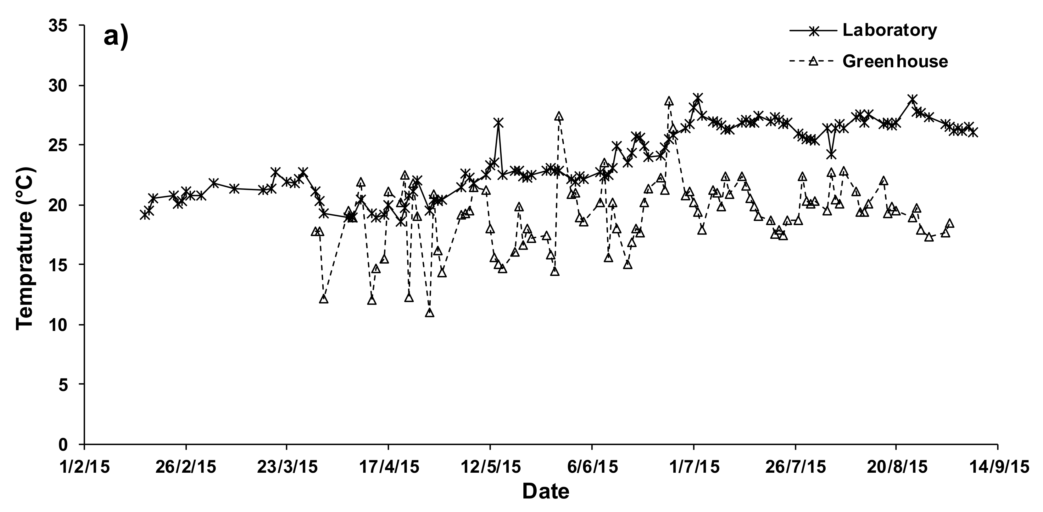
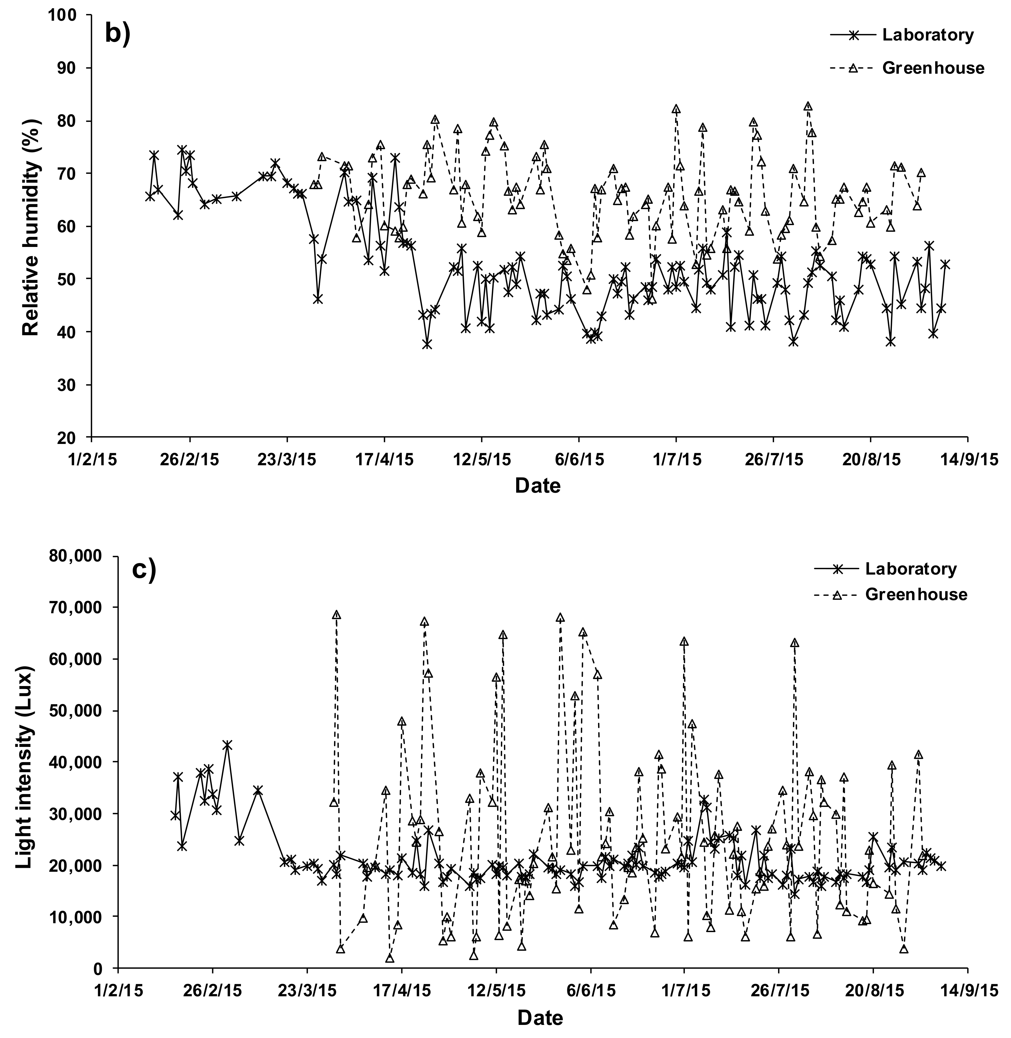
3.2. Growth Environmental Conditions

A comparison between the environmental boundary conditions in the laboratory and greenhouse associated with chilli plants grown in pots is shown in Figure 2. Temperature measurements complied with the recommended limits for different growth stages of chilli plants [55,75]. The observed temperature in the laboratory was slightly higher than in the greenhouse, especially for the summer season (Figure 2a). The recorded temperature in both locations met to the suggested range (24–29 °C) by Bhatt and Srinivasa [79] for the highest photosynthesis rate for various growth stages of chilli plants.

The mean values of relative humidity in the laboratory varied between 40 and 60%, and were lower than the humidity measurements in the greenhouse reaching 80% in July 2015 (Figure 2b). Low relative humidity may negatively impact the pollination process and the corresponding fruit development progress. In contrast, a high humidity causes fruit degradation and rotting [80]. High fluctuations of light intensity were monitored in the greenhouse compared to the steady light intensity in the laboratory at around 20,000 Lux (Figure 2c). An insufficient light intensity during the blossoming stage could seriously affect plant health and fruit productivity and quality, such as flower abscission [54]. Deli and Tiessen [81] recommended a light density range between 8600 and 17,200 Lux to avoid inhibition/detachment of flowers and other syndromes in plants.

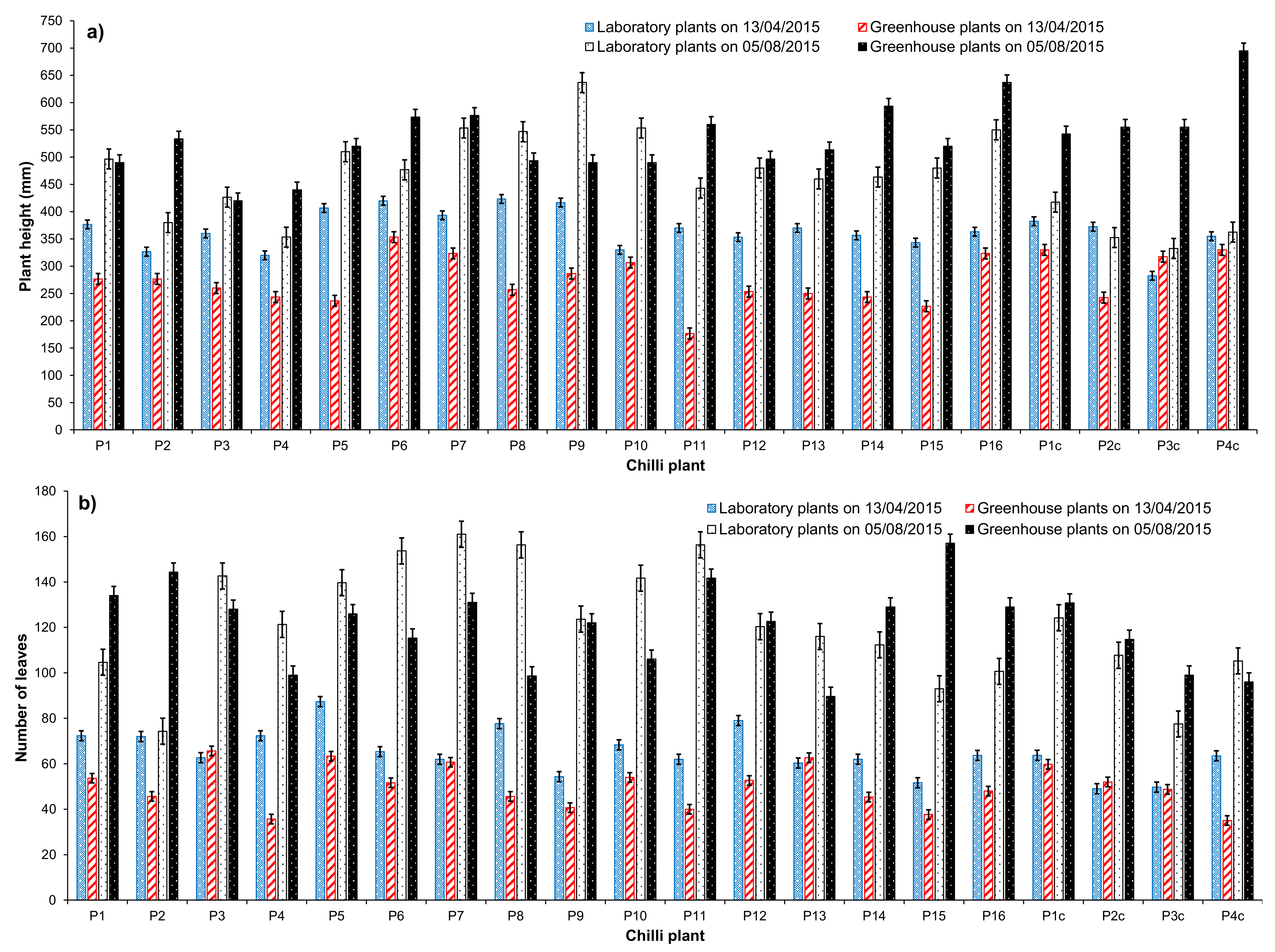
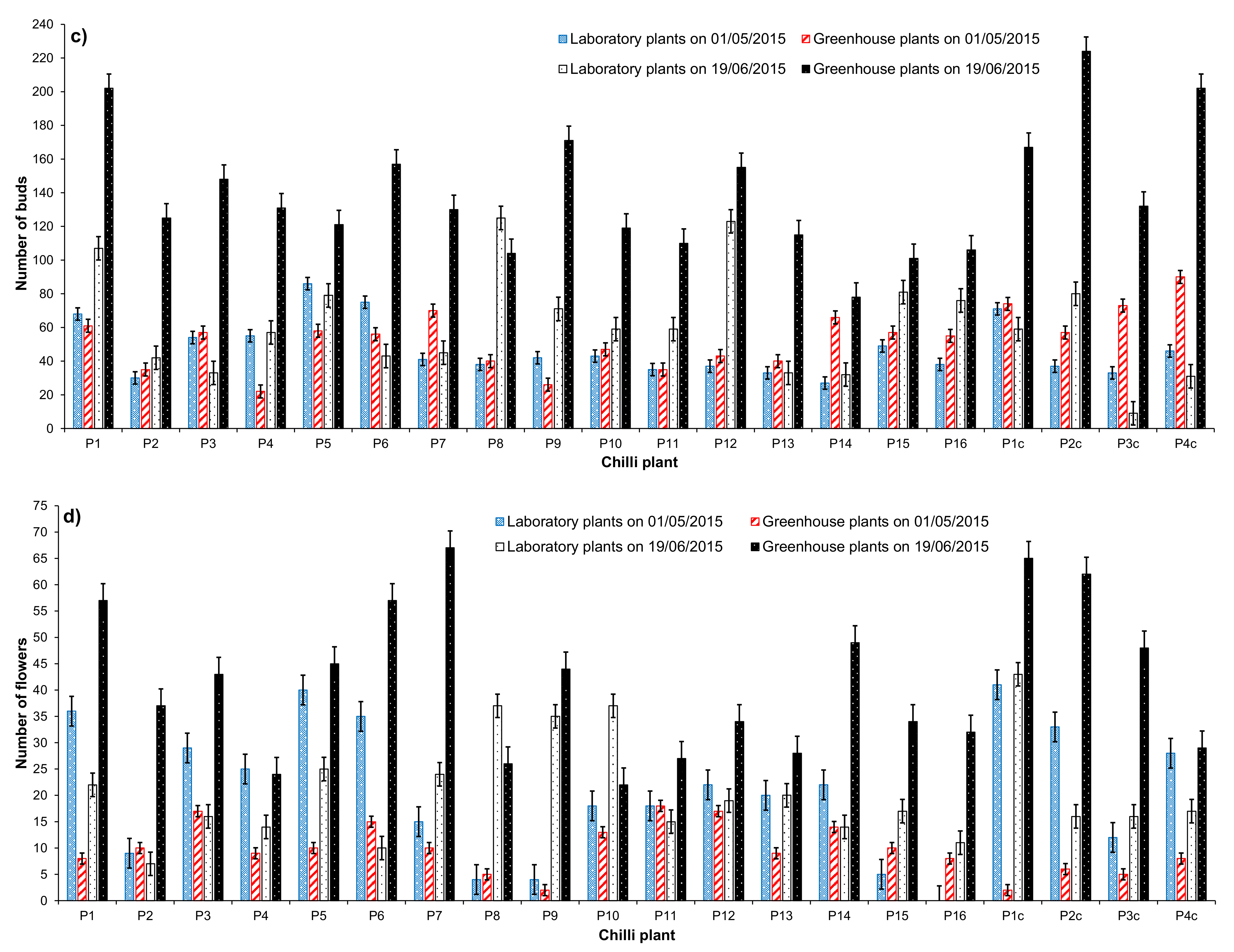
3.3. Growth Monitoring

Chilli plant biomass development was recorded in April and August 2015. Plant height and number of leaves considerably increased in April, while no significant increase (p > 0.05) in heights were observed after August. Old “fallen down” leaves and the growth of new ones were noticed in August.

In April 2015, the average heights of chilli plants grown in the laboratory were greater than the heights of the corresponding chilli group receiving the same irrigation water, but grown in the greenhouse (Figure 3a). The tallest plant in the laboratory was P8 with a height of 423 mm (watering by treated LC-SGW with only cement–ochre pellets; 2 days of HRT), while the shortest plant was P3c with a height of 283 mm (watering by tap water with only Phragmites australis; 2 days of HRT). In August 2015, chilli plants in the greenhouse showed a non-significant increase (p > 0.05) in height compared to corresponding plant heights in the laboratory. An exception was chilli plants receiving tap water. Chilli plants in both locations showed significant (p < 0.05) growth with good health in August compared to their growth rate measured in April.

The maximum average height in the greenhouse was recorded as 695 mm for P4c (receiving from system retaining tap water; 7 days HRT), which is significantly (p < 0.05) differed compared with other plants in the same location ranging between 420 and 695 mm. Only one significant record (p < 0.05) was linked to the height (637 mm) of the chilli plant P9 in the laboratory (watering by treated HC-SGW with only Phragmites australis; 7 days of HRT), which was greater than the corresponding plant height (490 mm) in the greenhouse, as shown in Figure 3a. The plant heights were between 333 and 637 mm with significant (p < 0.05) differences compared to each other.

In April, the counted numbers of chilli plant leaves were significantly (p < 0.05) greater than the number of leaves for plants grown in the greenhouse, except for P3, P7, P13, P1c, P2c, and P3c (Figure 3b). The number of leaves increased significantly (p > 0.05) for chilli plants in both places in August compared to April. A significant (p < 0.05) leaf count number in the greenhouse was noted for the plants P1, P2, P14, P15, P16, and P3c, which was greater than in the laboratory. In contrast, plants P3, P4, P5, P6, P7, P8, P10, and P13 had significantly (p < 0.05) less leaf numbers than in the laboratory (Figure 3b). The plant height measurements showed that the variation of irrigation water quality had significant effects on the development patterns for different weather conditions. Furthermore, the greenhouse conditions enhanced the plant biomass, particularly for plants receiving nutrients complying with the irrigation thresholds. These findings are in agreement with García-Delgado et al. [77], who stated that leaves, stems, and biomass productions of chilli plants significantly improved when irrigated with treated wastewater compared to other plants using other types of irrigation water with added mineral fertilizers in a greenhouse environment.

In April 2015, the number of chilli buds in the laboratory were significantly (p < 0.05) higher compared to the corresponding plants in the greenhouse, except for chilli plant P8 (Figure 3c). Then the number of buds fluctuated in both locations due to transformation to flowers or failure in growth (either slowly dying or even dropping), which was frequently noticed in the laboratory experiment. In May 2015, the bud numbers decreased approximately to half in both locations. In June 2015, chilli plants in the greenhouse showed new bud production. The bud numbers were significantly (p < 0.05) elevated compared to the laboratory plants, except for chilli plant P8, where the bud numbers were greater in the laboratory (Figure 3c). In July 2015, the counted number of buds decreased significantly (p < 0.05) in both locations compared to previous months, because of the production of flowers, except for plants P8 and P12, which still contained buds (Figure S1).

Blooming was observed first in the laboratory-based chilli plants by the middle of April 2015; a week later, it was also apparent for greenhouse plants. In May 2015, the counted flower numbers for plants located in the laboratory were significantly (p < 0.05) higher than in the greenhouse, except for plants P2, P8, P11, P15, and P16, where there were lower numbers. The maximum significant (p < 0.05) average number of flowers was recorded for plant P1c followed by plants P5 and P1 compared to other plants in the laboratory. In contrast to June 2015, greenhouse chilli plants produced significant (p < 0.05) numbers of flowers compared to the plants in the laboratory, with the exception of plants P8 and P10. The average flower number of plant P7 was significantly (p < 0.05) greater than the corresponding number of the other plants in the greenhouse (Figure 3d). In both locations, it was observed that the stage of producing flowers from buds was very rapid and it might occur within a few days, which agreed with previously published findings [54,78].

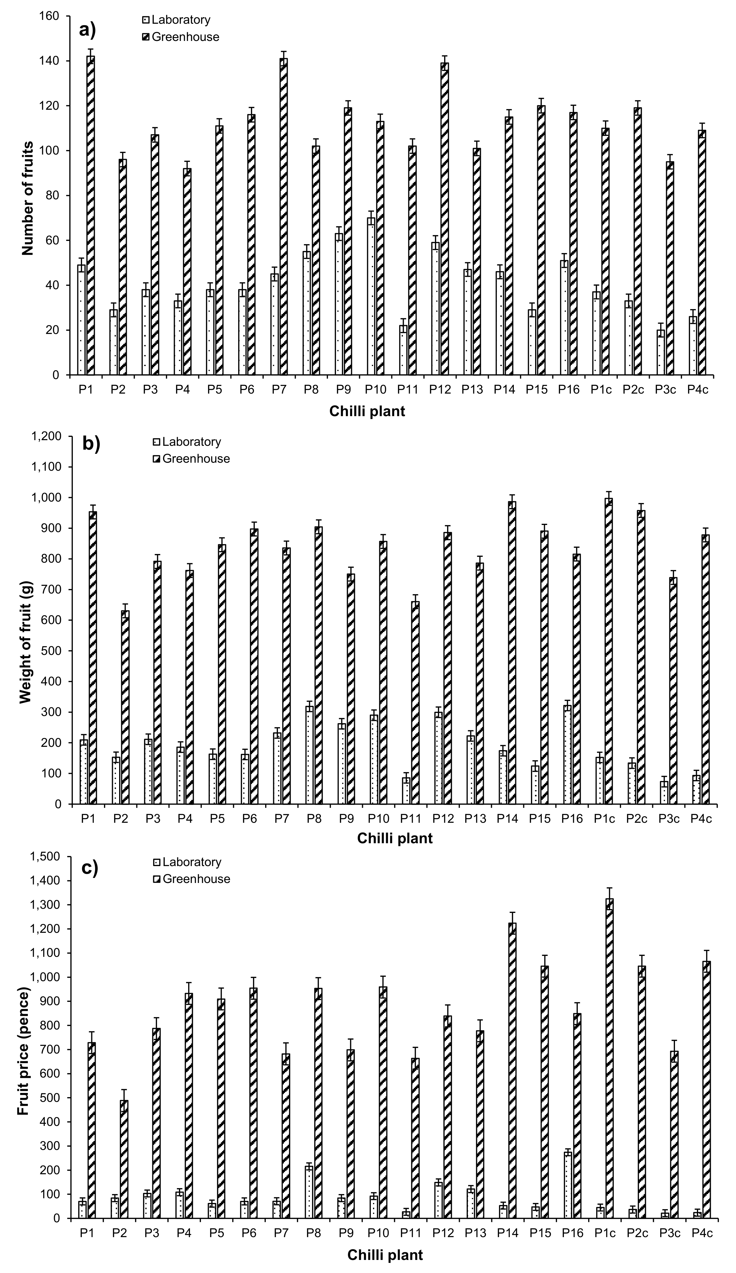
3.4. Chilli Fruit Production, Quality, and Classification

The production of chilli fruits was monitored from the ripening stage until the harvesting season. Following Almuktar et al. [54], chilli fruits were classified according to their quality, such as weight, length, width, and shape bending (

Table 4. Classification scheme for quality of the harvested chilli fruit [54].

Parameter	Class A	Class B	Class C	Class D	Class E
Quality class	Outstanding	Very good	Good	Satisfactory	Unsatisfactory
Approximate Codex Standard	“Extra” Class	Class I	Class II	Not applicable	Not applicable
Length (L, mm)	Very long (L ≥ 80)	Long (80 > L ≥ 60)	Medium (60 > L ≥ 40)	Short (40 > L ≥ 20)	Very short (L < 20)
Width (W, mm)	Very wide (W ≥ 20)	Wide (20 > W ≥ 16)	Medium (16 > W ≥ 12)	Slim (12 > W ≥ 8)	Very slim (W < 8)
Fresh weight (w, gram)	Very large (w ≥ 9)	Large (9 > w ≥ 7)	Medium (7 > w ≥ 5)	Small (5 > w ≥ 3)	Very small (w < 3)
Bending (L/W)	Characteristically (L/W ≥ 3.5)	Characteristically (L/W ≥ 3.5)	Characteristically (L/W ≥ 3.5)	Uncharacteristically (L/W < 3.5)	Uncharacteristically (L/W < 3.5)
Price (Sterling, pence/g)	2.00	1.00	0.50	0.25	0.00

). Therefore, the productivity of the chilli planting experiment was assessed depending on the number of produced fruits, their weight, and price. The chilli fruit price was estimated in pound sterling (GBP).

In both laboratory and greenhouse environments, harvesting of chilli fruits was commenced in June 2015 and finalised in January 2016. The monthly record showed that the maximum number of chilli fruits from both locations was harvested in July. The chilli fruit quantity in the greenhouse was 1512 fruits (12.024 kg), which was significantly (p < 0.05) higher than in the laboratory (254 fruits (1.384 kg)), as shown in Figure 4a,b. Plant P7 in the greenhouse and plant P8 in the laboratory contributed with the highest production of fruits in July: 104 (0.646 kg) and 29 (0.188 kg) chilli fruits, respectively. Plant P4c located in the greenhouse had the highest harvested weigh of fruits in July (0.787 kg for 86 chilli fruits) compared to all other plants in the greenhouse (Figure 4c,d). Furthermore, the chilli price in July linked to plant P8 in the laboratory was GBP 1.39 in comparison to the total price in July of GBP 6.57, which was significantly (p < 0.05) lower compared to the chilli price (GBP 10.75) associated with plant P1c in the greenhouse and to the total price of chilli fruits (GBP 135.58) gained only in July (Figure 4e,f).

The highest number of Class A produce was linked to plant P1c in the greenhouse (36 chillies of 0.449 kg worth GBP 8.97) compared to plant P16 in the laboratory (5 chillies), as shown in Figure 5 and Figure S2. Plant P1 grown in the greenhouse had a greater number of chilli fruits of Class B (47 chillies of 0.459 kg worth GBP 4.59) compared to plant P16 (13 chillies). Plants P12 and P2c in the greenhouse had the highest number of Class C fruits (35 chillies of total weight (price) of 0.214 kg (GBP 1.07) and 0.260 kg (GBP 1.33), respectively), compared to highest number of Class C fruits obtained in the laboratory from plant P8 (24 chillies). Class D chilli fruits was the dominant class for almost plants in both locations (Table 4). The highest number of Class D fruits was produced by plant P7 in greenhouse (52 chillies of 0.230 kg worth GBP 0.57) compared to the Class D fruits (33 chillies) from plant P10 located in the laboratory (Figure 5 and Figure S2). All plants in both locations produced Class E chilli fruits, which were deemed unsatisfactory, because they are very short, small and slim with little value on the market as fresh fruits (Table 4). Plant P11 in the greenhouse gave 31 chillies of Class E with a weight of 0.052 kg compared to 19 chillies from P10 in the laboratory.

A large number (142) of chilli fruits was produced from plant P1 in greenhouse; 47 fruits were labelled as Class B compared to 70 chillies from plant P10 in the laboratory (Figure 5a and Figure S2a). Plant P1c in the greenhouse produced the heaviest harvest of 0.998 kg; 0.449 kg was labelled as Class A fruits compared to 0.322 kg from plant P16 in the laboratory with 0.110 kg of Class B chillies (Figure 5b and Figure S2b). Regarding the chilli price, the highest income was obtained from P1c (GBP 13.25), where the majority of plants was linked to Class A produce (GBP 8.97), as shown in Figure 5c and Figure S2c. García-Delgado et al. [80] stated that chilli plants irrigated with treated wastewater produced a significantly high number of fruits, classified as large (70–90 mm in diameter) and very large (>90 mm in diameter) compared to groundwater and untreated wastewater with and without mineral fertilizer.

The total production of chilli fruits in the laboratory was 858 fruits where plants P10 and P9 gave large fruit numbers of 70 and 63 chillies, respectively, compared to other plants. These findings were greater than the average production number published by Almuktar et al. [54,82]. However, plants P16 and P8 in the laboratory produced the highest weights of 0.323 and 0.319 kg, respectively. The total chilli weight of 3.869 kg is linked to the laboratory planting experiment. The total produced quantity of chilli could be sold for GBP 17.61, where plants P16 and P8 chillies were priced as GBP 2.74 and GBP 2.16, respectively.

In the greenhouse, the total number of chill fruits harvested in the whole experiment was 2266 fruits with a total weight of 16.824 kg, which could be marketed for GBP 176.22. Plants P1 and P7 in the greenhouse produced the highest number of chillies of 142 and 141 fruits, respectively, but the highest chilli prices were indicated for plants P1c and P14 of GBP 13.25 and GBP 12.24 in this order. These figures are significantly higher than the ones published by Al-Isawi et al. [78].

A high fruit productivity in the greenhouse reflects the effect of real sunlight intensity, high relative humidity, and temperature, which contributed to enhanced soil and plant health, converting flowers to fruits more successfully compared to the boundary conditions of the laboratory [77].

The highest weight of chilli fruits was harvested from plants P1c, P14, P2c, and P8 with 0.997, 0.986, 0.958, and 0.905 kg, respectively. The highest chilli fruit numbers were associated with high nutrient availability for plant biomass production harvested from plants receiving effluent from T1 (floating wetland system treating greywater of high contamination level with a 2-day HRT in the presence of floating Phragmites australis), which agreed with findings reported by Al-Isawi et al. [78], in terms of nutrient load and hydraulic retention time. The results obtained from the greenhouse planting experiment were significantly better compared to the findings from the laboratory experiment in terms of chilli fruit quantity, quality, productivity, and marketability. However, chilli plants in the laboratory continued to produce fruits even after the usual harvest season.

Nutrients provided to the chilli plants by treated greywater and compost soil could be considered efficient for good harvesting. However, plant water consumption is related to the environmental weather conditions and growth stage, it is not strongly linked to the fruit productivity [3]. It was indicated that there was no significant difference in plant water consumption when comparing the laboratory to greenhouse plants [82].

Nutrients provided to the chilli plants by treated greywater and compost soil could be considered beneficial for a good harvest. However, the plant water consumption is related to the environmental and weather conditions as well as growth stage. It is not strongly linked to the fruit productivity [3]. Findings indicated that there was no significant difference in plant water consumption between laboratory and greenhouse plants [76].

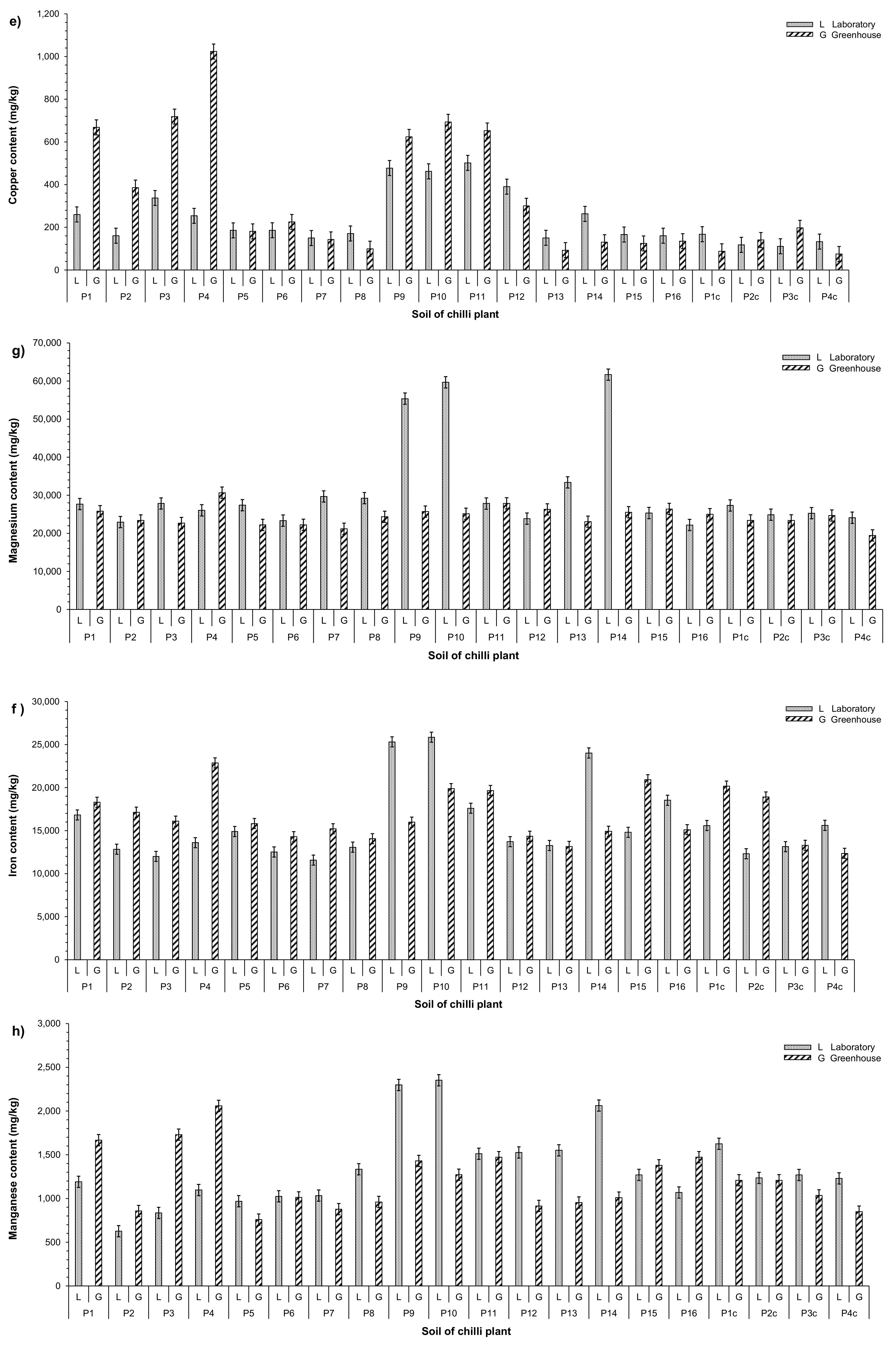
3.5. Accumulated Trace Elements in Soil

The findings of a comparison of detected trace elements for the collected soil samples from the laboratory and greenhouse experiments are illustrated in Figure 6. The chilli plant soils were fed with two different pollutant strengths of recycled greywater (Section 2.1). The chemical analysis of chilli plant soils for trace elements showed that significant changes happened in element concentrations compared to the raw soil. As described in Section 3.1, almost all water quality samples complied with irrigation water thresholds in terms of trace element concentrations, especially for the LC-SGW effluents. However, some samples related to HC-SGW effluents were not in compliance [1,11].

In general, the concentrations of accumulated trace elements in chilli plant soils for both the laboratory and greenhouse locations followed this trend: Mg > Fe > Al > Cr > Mn > Cd > Cu > B, with some variations in Cd, Cr, Cu, and Mn. The changes in trace element concentrations of organic media-based soil could be problematic to detect due to a high cation exchange capacity, leading to a high variety in chemical composition [83]. Furthermore, the bioavailability of the chemical elements as well as soil pH and organic content affect and govern plant uptake of soil elements [3]. The measured pH values of the chilli soil samples were around 6.5 to 8.5, especially for soils irrigated with LC-SGW. However, pH values less than 6.0 or greater than 8.5 were rarely recorded in soils, which were irrigated with tap water or HC-SGW, respectively. The allocated trace element ions from soil to plant tissue could be limited at a pH of around 7.0 or decreased at a pH greater than 6.5 [84].

Concentrations of Al in the laboratory plant soils irrigated with effluents of T9 (7-days HRT; HC-SWG; Phragmites australis), T10 (7-days HRT; HC-SWG), and T14 (7-days HRT; LC-SWG; Phragmites australis; cement–ochre pellets) were significantly higher (p < 0.05) than the Al concentrations of the other soils in both locations (Figure 6a). These effluents have relatively high pH values between 7.3 and 10.3. The soils of the control chilli plants that were irrigated with tap water (P1c, P2c, P3c, and P4c (Table 1)) showed Al concentrations between 6000 and 8000 mg/kg. Organic matter and clay proportions in agricultural soil govern the aluminium mobility and solubility at different soil pH conditions. A negative correlation was calculated between decreasing pH values and increasing aluminium ion exchange in soil. Then, Al mobility becomes limited to plant biomass with an abundance of Ca ions in soil [66]. There is no toxicity threat to human health and the environment associated with the accumulation of Al in soil or plants due to its low bioavailability. This element is present in high abundancy in organic soils, except for acid soils [3]. However, mineral contamination might be a risk when recycling wastewater in the agricultural environment. The build-up of chemicals, soil salinization, and mobilisation of pollutants from soil to cultivated crops should be monitored to protect the environment and consumers [38,80].

Traces of B were detected in all soils linked to chilli plants grown in the greenhouse, except for soil of chilli plant P7. In comparison, only eight of twenty soils with traces of B were found for plants grown in the laboratory (Figure 6b). A significantly higher concentration of B was observed in the soil of plants P3 (229.3 mg/kg) and P9 (180.7 mg/kg) grown in the laboratory and greenhouse, respectively. Soil samples of control plants, which were irrigated only with tap water, showed no trace of B. However, 55.3 mg/kg was detected in soil samples of P3c, which received water from the treatment system C3 (7-days HRT; tap water; Phragmites australis present). Planted soils irrigated with effluents from systems of 7-day HRT showed a high fluctuation in B concentration, in particular, those chillies grown in the greenhouse. Boron is present in soils associated with recycled effluents of treatment systems with long hydraulic retention times.

Significantly (p < 0.05) higher Cd, Cr, and Cu concentrations were detected in soils of chilli plants irrigated with effluents of HC-SGW compared to planted soils irrigated with LC-SGW. This is especially the case for those plants grown in the greenhouse. Recycling of effluents treated for longer hydraulic retention times showed less Cd, Cr, and Cu accumulations in soils irrigated with LC-SGW (Figure 6c–e). The accumulation of Cd, Cr, and Cu in soils watered with highly contaminated greywater was significant in greenhouse chilli plant soil. Concentrations were higher than the corresponding thresholds (Table 3).

The identified concentrations of Fe, Mg, and Mn in planted soils located in the laboratory and greenhouse were variable and fluctuated without a clear trend between 11,572 and 25,856 mg/kg for Fe, 19,455 and 61,667 mg/kg for Mg, and 626 and 2352 mg/kg for Mn. No significant effects were noted concerning the accumulations of Fe, Mg, and Mn in planted soil. However, the highest mineral concentrations were recorded for soil samples of plants P9, P10, and P14 grown in the laboratory: Fe (25,313, 25,856, and 24,023 mg/kg, respectively), Mg (55,376, 59,662, and 61,667 mg/kg, respectively) and Mn (2298, 2352, and 2063 mg/kg, respectively).

In comparison, Fe (22,871 mg/kg), Mg (mg/Kg), and Mn (2059 mg/kg) of soil linked to P4 grown in the greenhouse (Figure 6f–h) had the highest values (Table 3). A positive correlation between Fe and Mg was recorded, since Mg was consumed during plant photosynthesis. However, high Mg levels cause a low plant growth rate [66]. The build-up of chemicals, soil salinization, and soil pollutant mobilisation by cultivated crops negatively affect consumer health [38,80]. Oxygen and soil pH are crucial parameters for metal (e.g., Fe) bioavailability in terms of plant uptake and accumulation processes in their tissues influencing photosynthesis. Nevertheless, involving microorganisms in metal oxidative processes and metal hydroxide creation could limit metal consumption by plants [69,70].

Transfer rates of metals from soil to cultivated plants have been reported. They vary according to the following rank order: Cd > Cr > Ni > Zn > Cu > Mn [39]. The proportionate accumulation of trace elements in soil increases with irrigation of treated wastewater: Cd (109%), Cu (152%), Zn (32%), Ni (161%), and Cr (52.8%), crossing the maximum permissible threshold limits for long-term irrigation [85,86].

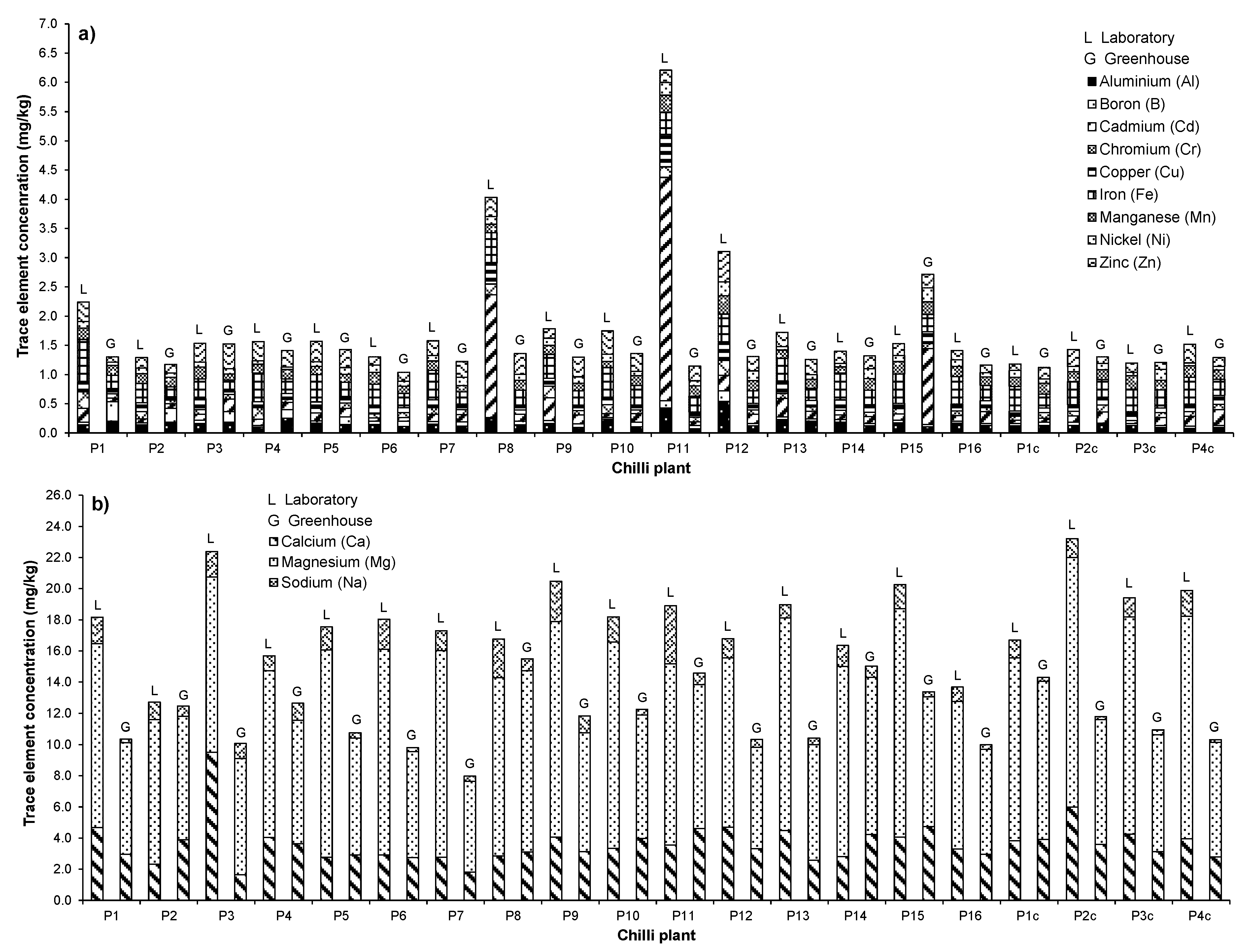
3.6. Accumulated Trace Elements in Chilli Fruits

Chilli fruits were analysed chemically for the accumulated concentrations of several minerals, including heavy metals (Table S2 and Figure 7). The statistical comparison of accumulated trace elements in chilli fruits is based on the effect of environmental growth conditions between the plants grown in the laboratory and greenhouse, and the effects of irritation water quality supplied to chilli plants (Table 1 and Table 2). The ranking order of occurrence for the trace element concentrations accumulated in chilli fruits grown in both the laboratory and greenhouse was as follows: Mg > Ca > Na > Fe > Zn > Al > Mn > Cu > Cd > Cr > Ni > B. The statistical analysis showed that the total accumulated chemical elements in chilli fruits of plants P11, P8, P12, and P1 grown in the laboratory were significantly (p < 0.05) higher than the accumulated concentrations in fruits of all chilli plants, and compared to, in particularly, plants grown in the greenhouse receiving water of the same quality (Table S2, Figure 7a,b). A greater accumulation of trace elements in the greenhouse was observed for chilli fruits of plant P15 (irrigated with effluent of treatment system T15; treating LC-SGW for 7-days HRT). The variation in environmental growth conditions affects the accumulation of trace elements in fruits. A high temperature was recorded in the laboratory and both high relative humidity and natural sunlight characterised the greenhouse environment [3,54,66,78,82,86,87]. Furthermore, chilli fruits of plant P15 grown in the greenhouse indicated a greater accumulation of Ca, Cd, Cu, Mn, and Ni with concentrations of 4.73, 1.30, 0.20, 0.21, and 0.24 mg/kg, respectively (Table S2).

Chilli fruits harvested from plant P12 in the laboratory (receiving water from treatment system T12; treating HC-SGW for 7-days HRT with cement–ochre pellets) showed greater accumulation of Al, B, Mn, Ni, and Zn with concentrations of 0.54, 0.18, 0.32, 0.24, and 0.52 mg/kg, respectively (Figure 7a,b). The highest concentrations of accumulated Cd (3.82 mg/ kg), Cu (0.56 mg/ kg), and Na (0.56 mg/ kg) were recorded in chilli fruits of plant P11 grown in the laboratory (receiving water from treatment system T11; treating HC-SGW for 7-days HRT). The notable accumulations of Cr and Fe with 0.28 and 0.75 mg/kg, correspondingly (Table S2), were found in the analysis of chilli fruits of plant P1 in the laboratory (irrigated with effluent of treatment T1; Treating HC-SGW for 2-days with Phragmites australis).

The maximum accumulated Al, B, Ca, Mg, and Na concentrations in chillies were 0.54, 0.33, 9.5, 16.02, and 3.72 mg/kg, respectively (Table S2). However, almost international guidelines and standards have not stated recommended limits for accumulated concentrations of Al, B, Ca, K, Mg, and Na (Table 3). Macronutrients (N, P, K, S, Ca, and Mg) and micronutrients, including heavy metals (Co, Cu, Fe, Mn, Mo, Ni, and Zn), must be provided to plants for healthy growth and are vital in human food. Soil deficiency could affect plant metabolism and biomass productivity [69]. However, high levels of micronutrients may cause plant toxicity and subsequently human and animal diseases [70]. In comparison with permissible chemical element concentrations (Table 3), the maximum detected concentrations of Cr, Cu, Fe, Mn, Ni, and Zn (0.28, 3.82, 0.75, 0.32, 0.25, and 0.52 mg/kg, as shown in Table S2) were significantly (p < 0.05) lower than the higher permissible limits for safe consumer health [27,31,32].

A significant maximum accumulated Cd concentration (3.82 mg/kg) was detected in chilli fruits of plant P11 grown in the laboratory. This plant received effluent from system T11 (storying high contamination greywater for 7days HRT). In comparison, the Cd concentration accumulated in chilli fruits grown in greenhouse and irrigated with the same water was only 0.06 mg/kg. The thresholds of allowable Cd concentrations accumulated in crops are 0.02 mg/kg [32], 0.05 mg/kg [31], and 0.1 mg/kg [27], as shown in Table 3. Therefore, fruits of the laboratory-grown plants P1, P8, P9, P11, P12, and P13 crossed the allowable Cd limits significantly (p < 0.05): 0.24, 2.10, 0.39, 3.82, 0.26, and 0.31 mg/kg, respectively. In the greenhouse, chilli fruits of P3, P15, P16, and P4c (control plant receiving tap water) showed Cd level significantly (p < 0.05) higher than the corresponding thresholds with accumulated concentrations of 0.22, 1.30, 0.21, and 0.27 mg/kg in that order. It follows that greenhouse plants much less accumulated Cd and were safer for human health. The fixation of Cd in soils (similar for F, Hg, and Pb, which were not considered in this study) is often associated with contaminated air, applying certain phosphoric fertilizers to agricultural soils, and Cd being present in irrigation water [86]. Accumulated trace element concentrations may be greater than the safe thresholds for soils, vegetable leaves, and fruits due to irrigation with treated wastewater [39,86] or cultivated in contaminated soil associated with mining areas [73].

4. Conclusions and Recommendations

Greywater and wastewater treatment systems, such as all types of constructed wetlands, can provide effluents to be recycled for irrigation. The best crop yield results and plant health could be achieved by following the international guidelines to control microbial and mineral pollutions associated with recycling of wastewater to protect human health and the environment. Total suspended and dissolved solids in irrigation water cause problems for both soil and cultivated plants.

Environmental conditions had a significant effect on plant growth, fruit quality, productivity, and marketability. Greenhouse-grown chilli plants had more acceptable yields, since the corresponding environmental boundary conditions (mainly humidity and sunlight) were more optimal than in the laboratory. Chilli plants irrigated with the same greywater in terms of quality and quantity gave significantly different yields for the two different weather conditions. The trace element accumulation in plant soil was reduced, except for cadmium and chromium. There was also less accumulation of trace elements in chilli fruits grown in the greenhouse. However, accumulated cadmium concentrations were above the permissible maximum thresholds.

The percentage of buds that developed to chilli fruits in the greenhouse was significantly higher in comparison to the laboratory experiment. Irrigation of chillies planted in the greenhouse achieved high marketability with high physical quality of fruits compared to laboratory-grown plants. The accumulation of some metals within the soil threatens plants and subsequently human health. Nevertheless, the accumulation of almost all heavy metals in the soil and plant tissues was less than the permissible thresholds. The trace element accumulation in chilli fruits grown in the laboratory was greater than in the greenhouse. The accumulated Cd in chilli fruits of plants grown in the laboratory was higher than the threshold. However, the risk of mineral contamination by accumulation of heavy metals in soils and chilli fruits must be reduced by optimising the greywater treatment system.

Treatment technology designated for irrigation water should comprise of stages for heavy metal removal. It is recommended to allow up to 12 h for solids in effluents to settle, when the total suspended solid concentration is above 20 mg/L in the irrigation water and the relatively low microbial growth is determined. High total suspended and dissolved solids concentrations could cause clogging of soil and negatively affect the soil structure and permeability. Floating treatment systems could be improved by increasing the macrophyte density. Furthermore, it is recommended to assess organic contaminations, such as toxic polycyclic aromatic hydrocarbons in chilli fruits.

References

1. FAO. User Manual for Irrigation with Treated Wastewater; Food and Agriculture Organization (FAO) of the United Nations, Regional Office for Near East: Cairo, Egypt, 2003. [Google Scholar]
2. WHO. Guidelines for the Safe Use of Wastewater, Excreta and Greywater: Wastewater Use in Agriculture; World Health Organization (WHO): Geneva, Switzerland, 2006; Volume 2. [Google Scholar]
3. Almuktar, S.A.A.A.N.; Abed, S.N.; Scholz, M. Contaminations of Soil and Two Capsicum annuum Generations Irrigated by Reused Urban Wastewater Treated by Different Reed Beds. Int. J. Environ. Res. Public Health 2018, 15, 1776. [Google Scholar] [CrossRef] [Green Version]
4. Almuktar, S.A.A.A.N.; Abed, S.N.; Scholz, M. Wetlands for wastewater treatment and subsequent recycling of treated effluent: A review. Environ. Sci. Pollut. Res. 2018, 25, 23595–23623. [Google Scholar] [CrossRef] [PubMed] [Green Version]
5. DESA-UN. World Population Prospects 2019: Highlights; Report (ST/ESA/SER.A/423); United Nations, Department of Economic and Social Affairs, Population Division: New York, NY, USA, 2019. [Google Scholar]
6. Alcamo, J.; Döll, P.; Kaspar, F.; Stefan, S. Global Change and Global Scenarios of Water Use and Availability: An Application of WaterGAP 1.0; Centre for Environmental Systems Research, University of Kassel: Kassel, Germany, 1997. [Google Scholar]
7. Alcamo, J.; Henrichs, T.; Rösch, T. World Water in 2025: Global Modelling and Scenario Analysis for the World Commission on Water for the 21st Century; Centre for Environmental Systems Research, University of Kassel: Kassel, Germany, 2000. [Google Scholar]
8. Scheierling, S.M.; Bartone, C.R.; Mara, D.D.; Drechsel, P. Towards an agenda for improving wastewater use in agriculture. Water Int. 2011, 36, 420–440. [Google Scholar] [CrossRef]
9. WWAP-UN. The United Nations World Water Development Report 4: Managing Water Under Uncertainty and Risk; UNESCO, World Water Assessment Programme (WWAP): Paris, France, 2012. [Google Scholar]
10. WHO. Health Guidelines for the Use of Wastewater in Agriculture and Aquaculture; Technical Report Series No. 77; World Health Organization (WHO): Geneva, Switzerland, 1989. [Google Scholar]
11. USEPA. Guidelines for Water Reuse; Report (EPA/600/R-12/618); United States Environmental Protection Agency (USEPA): Washington, DC, USA, 2012. [Google Scholar]
12. Cirelli, G.L.; Consoli, S.; Licciardello, F.; Aiello, R.; Giuffrida, F.; Leonardi, C. Treated municipal wastewater reuse in vegetable production. Agric. Water Manag. 2012, 104, 163–170. [Google Scholar] [CrossRef]
13. Willer, H.; Lernoud, J. The World of Organic Agriculture. Statistics and Emerging Trends; Research Institute of Organic Agriculture (FiBL), Frick, and IFOAM–Organics International: Bonn, Germany, 2019. [Google Scholar]
14. Weissengruber, L.; Möller, K.; Puschenreiter, M.; Friedel, J.K. Long-term soil accumulation of potentially toxic elements and selected organic pollutants through application of recycled phosphorus fertilizers for organic farming conditions. Nutr. Cycl. Agroecosyst. 2018, 110, 427–449. [Google Scholar] [CrossRef] [Green Version]
15. UNESCO. Water for People-Water for Life: A Joint Report by the Twenty-Three United Nations Agencies Concerned with Freshwater; United Nations Educational, Scientific and Cultural Organization (UNESCO): Barcelona, Spain, 2003. [Google Scholar]
16. Shuval, H.I.; Adin, A.; Fattal, B.; Rawitz, E.; Yekutiel, P. Wastewater Irrigation in Developing Countries: Health Effects and Technical Solutions; Technical Paper No. 51; World Bank: Washington, DC, USA, 1986. [Google Scholar]
17. Dalahmeh, S.; Baresel, C. Reclaimed Wastewater Use Alternatives and Quality Standards from Global to Country Perspective: Spain versus Abu Dhabi Emirate; IVL Swedish Environmental Research Institute: Uppsala/Stockholm, Sweden, 2014. [Google Scholar]
18. Toze, S. Reuse of effluent water–Benefits and risks. Agric. Water Manag. 2006, 80, 147–159. [Google Scholar] [CrossRef] [Green Version]
19. Nolde, E. Greywater reuse systems for toilet-flushing in multi-storey buildings-over ten years’ experience in Berlin. Urban Water 1999, 1, 275–284. [Google Scholar] [CrossRef]
20. Christova-Boal, D.; Eden, R.E.; McFarlane, S. An investigation into greywater reuse for urban residential properties. Desalination 1996, 106, 391–397. [Google Scholar] [CrossRef]
21. Eriksson, E.; Auffarth, K.; Henze, M.; Ledin, A. Characteristics of grey wastewater. Urban Water 2002, 4, 85–104. [Google Scholar] [CrossRef]
22. Al-Jayyousi, O.R. Greywater reuse: Towards sustainable water management. Desalination 2003, 156, 181–192. [Google Scholar] [CrossRef]
23. Edogbo, B.; Okolocha, E.; Maikai, B.; Aluwong, T.; Uchendu, C. Risk Analysis of Heavy Metal Contamination in Soil, Vegetables and Fish around Challawa Area in Kano State, Nigeria. Sci. Afr. 2020, 17, e00281. [Google Scholar] [CrossRef]
24. Hussain, M.I.; Qureshi, A.S. Health risks of heavy metal exposure and microbial contamination through consumption of vegetables irrigated with treated wastewater at Dubai, UAE. Environ. Sci. Pollut. Res. 2020, 27, 11213–11226. [Google Scholar] [CrossRef]
25. Osmani, M.; Bani, A.; Hoxha, B. Heavy Metals and Ni Phytoextraction in the Metallurgical Area Soils in Elbasan. Albanian J. Agric. Sci. 2015, 14, 414–419. [Google Scholar]
26. Mkhinini, M.; Boughattas, I.; Alphonse, V.; Livet, A.; Gıustı-Mıller, S.; Bannı, M.; Bousserrhıne, N. Heavy metal accumulation and changes in soil enzymes activities and bacterial functional diversity under long-term treated wastewater irrigation in East Central region of Tunisia (Monastir governorate). Agric. Water Manag. 2020, 235, 106–150. [Google Scholar] [CrossRef]
27. FAO/WHO. Codex Committee on Contaminants in Foods 10th Session; Working Document for Information and Use in Discussions Related to Contaminants and Toxins in the GSCTFF Volume 4; Food and Agriculture Organization, Rome, Italy 2016. Available online: http://www.fao.org/fao-who-codexalimentarius (accessed on 9 August 2021).
28. Hadayat, N.; De Oliveira, L.M.; Da Silva, E.; Han, L.; Hussain, M.; Liu, X.; Ma, L.Q. Assessment of trace metals in five most-consumed vegetables in the US: Conventional vs. organic. Environ. Pollut. 2018, 243, 292–300. [Google Scholar] [CrossRef] [PubMed]
29. Awashthi, S.K. Prevention of Food Adulteration Act No 37 of 1954; Central and State Rules as Amended for 1999; Ashoka Law House: New Delhi, India, 2000. [Google Scholar]
30. NHFPC. GB 2762-2012 China Food Safety National Standard for Maximum Levels of Contaminants in Foods; NHFPC-National Health and Family Planning of People’s Republic of China: Beijing, China, 2012. [Google Scholar]
31. European Union (EU). Heavy Metals in Wastes, European Commission on Environment; European Union: Brussels, Belgium, 2002; Available online: http://ec.europa.eu/environment/waste/studies/pdf/heavymetalsreport.pdf (accessed on 9 August 2021).
32. WHO. Permissible Limits of Heavy Metals in Soil and Plants; World Health Organization (WHO): Geneva, Switzerland, 1996. [Google Scholar]
33. Douay, F.; Pelfrêne, A.; Planque, J.; Fourrier, H.; Richard, A.; Roussel, H.; Girondelot, B. Assessment of potential health risk for inhabitants living near a former lead smelter. Part 1: Metal concentrations in soils, agricultural crops, and home grown vegetables. Environ. Monit. Assess. 2013, 185, 3665–3680. [Google Scholar] [CrossRef]
34. Hu, J.; Wu, F.; Wu, S.; Cao, Z.; Lin, X.; Wong, M.H. Bioaccessibility, dietary exposure and human risk assessment of heavy metals from market vegetables in Hong Kong revealed with an in vitro gastrointestinal model. Chemosphere 2013, 91, 455–461. [Google Scholar] [CrossRef]
35. Zhou, H.; Yang, W.T.; Zhou, X.; Liu, L.; Gu, J.F.; Wang, W.L.; Zou, J.L.; Tian, T.; Peng, P.Q.; Liao, B.H. Accumulation of heavy metals in vegetable species planted in contaminated soils and the health risk assessment. Int. J. Environ. Res. Public Health 2016, 13, 289. [Google Scholar] [CrossRef] [PubMed] [Green Version]
36. Bigdeli, M.; Seilsepour, M. Investigation of metals accumulation in some vegetables irrigated with waste water in Shahre Rey-Iran and toxicological implications. Am.-Eurasian J. Agric. Environ. Sci. 2008, 4, 86–92. [Google Scholar]
37. Shaheen, N.; Irfan, N.M.; Khan, I.N.; Islam, S.; Islam, M.S.; Ahmed, M.K. Presence of heavy metals in fruits and vegetables: Health risk implications in Bangladesh. Chemosphere 2016, 152, 431–438. [Google Scholar] [CrossRef] [PubMed]
38. Khan, S.; Cao, Q.; Zheng, Y.M.; Huang, Y.Z.; Zhu, Y.G. Health risks of heavy metals in contaminated soils and food crops irrigated with wastewater in Beijing, China. Environ. Pollut. 2008, 152, 686–692. [Google Scholar] [CrossRef]
39. Khan, K.; Lu, Y.; Khan, H.; Ishtiaq, M.; Khan, S.; Waqas, M.; Wei, L.; Wang, T. Heavy metals in agricultural soils and crops and their health risks in Swat District, northern Pakistan. Food Chem. Toxicol. 2013, 58, 449–458. [Google Scholar] [CrossRef]
40. Scholz, M.; Lee, B.H. Constructed wetlands: A review. Int. J. Environ. Stud. 2005, 62, 421–447. [Google Scholar] [CrossRef]
41. Vymazal, J. Removal of nutrients in various types of constructed wetlands. Sci. Total Environ. 2007, 380, 48–65. [Google Scholar] [CrossRef] [PubMed]
42. Scholz, M. Sustainable Water Treatment: Engineering Solutions for a Variable Climate; Elsevier Inc.: Amsterdam, The Netherlands, 2019. [Google Scholar]
43. Brix, H. Use of constructed wetlands in water pollution control: Historical development, present status, and future perspectives. Water Sci. Technol. 1994, 30, 209–224. [Google Scholar] [CrossRef] [Green Version]
44. Vymazal, J. Horizontal sub-surface flow and hybrid constructed wetlands systems for wastewater treatment: Review. Ecol. Eng. 2005, 25, 478–490. [Google Scholar] [CrossRef]
45. Scholz, M. Wetland Systems–Storm Water Management Control; Springer: Berlin, Germany, 2010. [Google Scholar]
46. Borne, K.E.; Fassman-Beck, E.A.; Tanner, C.C. Floating treatment wetland retrofit to improve stormwater pond performance for suspended solids, copper and zinc. Ecol. Eng. 2013, 54, 173–182. [Google Scholar] [CrossRef]
47. Wang, C.Y.; Sample, D.J. Assessment of the nutrient removal effectiveness of floating treatment wetlands applied to urban retention ponds. J. Environ. Manag. 2014, 137, 23–35. [Google Scholar] [CrossRef]
48. Keizer-Vlek, H.E.; Verdonschot, P.F.M.; Verdonschot, R.C.M.; Dekkers, D. The contribution of plant uptake to nutrient removal by floating treatment wetlands. Ecol. Eng. 2014, 73, 684–690. [Google Scholar] [CrossRef]
49. Rezania, S.; Taib, S.M.; Din, M.F.M.; Dahalan, F.A.; Kamyab, H. Comprehensive review on phytotechnology: Heavy metals removal by diverse aquatic plants species from wastewater. J. Hazard. Mater. 2016, 318, 587–599. [Google Scholar] [CrossRef]
50. Abed, S.N.; Scholz, M. Chemical simulation of greywater. Environ. Technol. 2016, 37, 1631–1646. [Google Scholar] [CrossRef] [PubMed]
51. Abed, S.N.; Almuktar, S.A.A.A.N.; Scholz, M. Phytoremediation performance of floating treatment wetlands with pelletized mine water sludge for synthetic greywater treatment. J. Environ. Health Sci. Eng. 2019, 372, 1–28. [Google Scholar] [CrossRef] [Green Version]
52. Abed, S.N.; Almuktar, S.A.A.A.N.; Scholz, M. Remediation of synthetic greywater in mesocosm-scale floating treatment wetlands. Ecol. Eng. 2017, 102, 303–319. [Google Scholar] [CrossRef]
53. Abed, S.N.; Almuktar, S.A.A.A.N.; Scholz, M. Treatment of contaminated greywater using pelletised mine water sludge. J. Environ. Manag. 2017, 197, 10–23. [Google Scholar] [CrossRef]
54. Almuktar, S.A.A.A.N.; Scholz, M.; Al-Isawi, R.; Sani, A. Recycling of domestic wastewater treated by vertical-flow wetlands for watering of vegetables. Water Pract. Technol. 2015, 10, 445–464. [Google Scholar] [CrossRef]
55. Nickels, J. Growing Chillies—A Guide to the Domestic Cultivation of Chilli Plants; Jason Nickels: London, UK, 2012. [Google Scholar]
56. Jones, J.B., Jr. Instructions for Growing Tomatoes in the Garden and Greenhouse; GroSystems: Anderson, SC, USA, 2013. [Google Scholar]
57. APHA. Standard Methods for the Examination of Water and Wastewater, 21st ed.; American Public Health Association (APHA), American Water Works Association, and Water and Environment Federation: Washington, DC, USA, 2005. [Google Scholar]
58. USEPA. SW–846: Test method 6010D: Inductively Coupled Plasma-Optical Emission Spectrometry (ICP-OES); Revision 4; United States Environmental Protection Agency (USEPA): Washington, DC, USA, 2014. [Google Scholar]
59. USEPA. Method 200.7: Determination of Metals and Trace Elements in Water and Wastes by Inductively Coupled Plasma-Atomic Emission Spectrometry; Revision 4.4; United States Environmental Protection Agency (USEPA): Washington, DC, USA, 1994. [Google Scholar]
60. Chary, N.S.; Kamala, C.T.; Raj, D.S.S. Assessing risk of heavy metals from consuming food grown on sewage irrigated soils and food chain transfer. Ecotoxicol. Environ. Saf. 2008, 69, 513–524. [Google Scholar] [CrossRef]
61. USEPA. Method 3050B: Acid Digestion of Sediments, Sludges, and Soils; Revision 2; United States Environmental Protection Agency (USEPA): Washington, DC, USA, 1996. [Google Scholar]
62. Plank, C.O. Plant Analysis Reference Procedures for the Southern Region of the United States.; Southern Cooperative Series Bulletin number 368; University of Georgia: Athens, GA, USA, 1992. [Google Scholar]
63. Shapiro, S.S.; Wilk, M.B. An analysis of variance test for normality (complete samples). Biometrika 1965, 52, 591–611. [Google Scholar] [CrossRef]
64. Kasuya, E. Mann-Whitney U test when variances are unequal. Anim. Behav. 2001, 61, 1247–1249. [Google Scholar] [CrossRef] [Green Version]
65. Stoline, M.R. The status of multiple comparisons: Simultaneous estimation of all pairwise comparisons in one-way ANOVA designs. Am. Stat. 1981, 35, 134–141. [Google Scholar]
66. Almuktar, S.A.A.A.N.; Scholz, M. Mineral and biological contamination of soil and Capsicum annuum irrigated with recycled domestic wastewater. Agric. Water Manag. 2016, 167, 95–109. [Google Scholar] [CrossRef]
67. Decreto Ministeriale. Regulating Technical Standards for Wastewater Reuse; Decreto Ministeriale: Rome, Italy, 2003; Volume 185. [Google Scholar]
68. Bar-Tal, A.; Aloni, B.; Karni, L.; Rosenberg, R. Nitrogen nutrition of greenhouse pepper. II. Effects of nitrogen concentration and NO3:NH4 ratio on growth, transpiration, and nutrient uptake. HortScience 2001, 36, 1252–1259. [Google Scholar] [CrossRef]
69. Millaleo, R.; Reyes-Díaz, M.; Ivanov, A.; Mora, M.; Alberdi, M. Manganese as essential and toxic element for plants: Transport, accumulation and resistance mechanisms. J. Soil Sci. Plant Nutr. 2010, 10, 470–481. [Google Scholar] [CrossRef] [Green Version]
70. McCauly, A.; Jones, C.; Jacobsen, J. Plant Nutrient Functions and Deficiency and Toxicity Symptoms; Nutrient Management Module No. 9; Montana State University: Bozeman, MT, USA, 2011. [Google Scholar]
71. BOE. Royal Decree 140/2003 That Establish Health Criteria of Water Quality for Human Consumption; Boletín Oficial de Estado (BOE) No 45, 21/02/2003; BOE: Madrid, Spain, 2003. [Google Scholar]
72. Ewers, U. Standards, guidelines and legislative regulations concerning metals and their compounds. In Metals and Their Compounds in the Environment: Occurrence, Analysis and Biological Relevance; Merian, E., Ed.; VCH: Weinheim, Germany, 1991; pp. 458–468. [Google Scholar]
73. NJDEP. Soil Cleanup Criteria; Proposed Cleanup Standards for Contaminated Sites, NJAC 7:26D; New Jersey Department of Environmental Protection: Tuckerton, NJ, USA, 1996. [Google Scholar]
74. DPR-EGASPIN. Environmental Guidelines and Standards for the Petroleum Industry in Nigeria (EGASPIN); Department of Petroleum Resources: Lagos, Nigeria, 2002. [Google Scholar]
75. Almuktar, S.A.A.A.N.; Scholz, M.; Al-Isawi, R.H.K.; Sani, A. Recycling of domestic wastewater treated by vertical-flow wetlands for irrigating Chillies and Sweet Peppers. Agric. Water Manag. 2015, 149, 1–22. [Google Scholar] [CrossRef]
76. Pinto, U.; Maheshwari, B.L.; Grewal, H.S. Effects of greywater irrigation on plant growth, water use and soil properties. Resour. Conserv. Recycl. 2010, 54, 429–435. [Google Scholar] [CrossRef]
77. García-Delgado, C.; Eymar, E.; Contreras, J.I.; Segura, M.L. Effects of fertigation with purified urban wastewater on soil and pepper plant (Capsicum annuum L.) production, fruit quality and pollutant contents. Span. J. Agric. Res. 2012, 10, 209–221. [Google Scholar] [CrossRef] [Green Version]
78. Al-Isawi, R.H.; Scholz, M.; Al-Faraj, F.A. Assessment of diesel-contaminated domestic wastewater treated by constructed wetlands for irrigation of chillies grown in a greenhouse. Environ. Sci. Pollut. Res. 2016, 23, 25003–25023. [Google Scholar] [CrossRef] [PubMed] [Green Version]
79. Bhatt, R.M.; Rao, N.K.S. Photosynthesis and dry matter partitioning in three cultivars of Capsicum annuum L. grown at two temperature conditions. Photosynthetica 1989, 23, 21–26. [Google Scholar]
80. Almuktar, S.A.A.A.N.; Abed, S.N.; Scholz, M. Recycling of domestic wastewater treated by vertical-flow wetlands for irrigation of two consecutive Capsicum annuum generations. Ecol. Eng. 2017, 107, 82–98. [Google Scholar] [CrossRef]
81. Deli, J.; Tiessen, H. Interaction of temperature and light intensity on flowering of Capsicum frutescens var grossum cv. California Wonder. J. Am. Soc. Hortic. Sci. 1969, 94, 349–351. [Google Scholar]
82. Al-Isawi, R.H.; Almuktar, S.A.A.A.N.; Scholz, M. Monitoring and assessment of treated river, rain, gully pot and grey waters for irrigation of Capsicum annuum. Environ. Monit. Assess. 2016, 188, 287. [Google Scholar] [CrossRef] [PubMed] [Green Version]
83. Ding, Z.; Li, Y.; Sun, Q.; Zhang, H. Trace elements in soils and selected agricultural plants in the Tongling mining area of China. Int. J. Environ. Res. Public Health 2018, 15, 202. [Google Scholar] [CrossRef] [Green Version]
84. Sharma, R.K.; Agrawal, M.; Marshall, F. Heavy metal contamination in vegetables grown in wastewater irrigated areas of Varanasi, India. Bull. Environ. Contam. Toxicol. 2006, 77, 312–318. [Google Scholar] [CrossRef] [PubMed]
85. Singh, A.; Sharma, R.K.; Agrawal, M.; Marshall, F.M. Risk assessment of heavy metal toxicity through contaminated vegetables from waste water irrigated area of Varanasi, India. Trop. Ecol. 2010, 51, 375–387. [Google Scholar]
86. Wuana, R.A.; Okieimen, F.E. Heavy metals in contaminated soils: A review of sources, chemistry, risks and best available strategies for remediation. Int. Sch. Res. Net. ISRN Ecol. 2011, 2011, 1–20. [Google Scholar] [CrossRef] [Green Version]
87. Chemicals, H. Crop Guide: Peppers; Haifa Group: Haifa, Israel, 2019; Available online: https://www.haifa-group.com/articles/crop-guide-peppers/ (accessed on 9 August 2021).
Figure 1. Photographs (taken by Suhad Almuktar) of chilli plants (Capsicum annuum L.) stages: (a) seedlings grown in propagators; (b) seedlings transplanted in large pots; (c) laboratory-controlled experiment; and (d) greenhouse-based semi-controlled experiment.
Agronomy 11 01817 g001aAgronomy 11 01817 g001b
Figure 2. Monitoring growth environmental condition for growth chilli plant in laboratory and greenhouse in terms of (a) temperature; (b) relative humidity; and (c) light intensity.
Agronomy 11 01817 g002aAgronomy 11 01817 g002b
Figure 3. Monitoring of chilli plant growth in terms of (a) plant height; (b) number of leaves; (c) number of buds; and (d) number of flowers.
Agronomy 11 01817 g003aAgronomy 11 01817 g003b
Figure 4. Monthly fruit harvest and productivity of chilli plants grown in laboratory and greenhouse environments in terms of (a,b) number of fruits; (c,d) weight of fruit; and (e,f) fruit price.
Agronomy 11 01817 g004
Figure 5. Overall fruit productivity of chilli plants grown in laboratory and greenhouse environments in terms of (a) number of fruits; (b) weight of fruits; and (c) fruit price.
Agronomy 11 01817 g005
Figure 6. Comparison between the content of accumulated trace elements in the soil of chilli plants grown in the laboratory and greenhouse environments in terms of (a) aluminium; (b) boron; (c) cadmium; (d) chromium, (e) copper; (f) iron; (g) magnesium; and (h) manganese.
Agronomy 11 01817 g006aAgronomy 11 01817 g006b
Figure 7. Comparison between trace element concentrations identified in chilli fruits grown in laboratory and greenhouse environments for (a) aluminium, boron, cadmium, chromium, copper, iron, manganese, nickel and zinc; and (b) calcium, magnesium, and sodium.
Agronomy 11 01817 g007