
Towards the Use of Land Use Legacies in Landslide Modeling: Current Challenges and Future Perspectives in an Austrian Case Study

 , , ,
, , ,
Abstract
:1. Introduction
2. Materials and Methods
2.1. Study Area
2.2. Data
2.2.1. Land Surface Data
2.2.2. LULC Legacy
2.2.3. Airborne LiDAR-Derived Landslide Inventories
2.3. Methods
2.3.1. Landslide Susceptibility Modeling Design
2.3.2. Assessment of the Effect of Land Use Legacy
3. Results
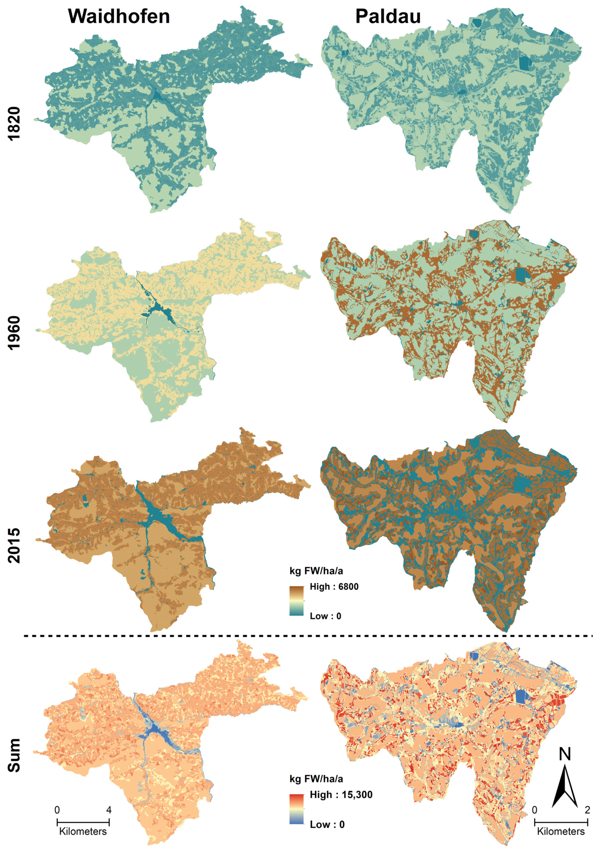
3.1. LULC Change
3.2. LULC Legacy Effects on Landslide Occurrence
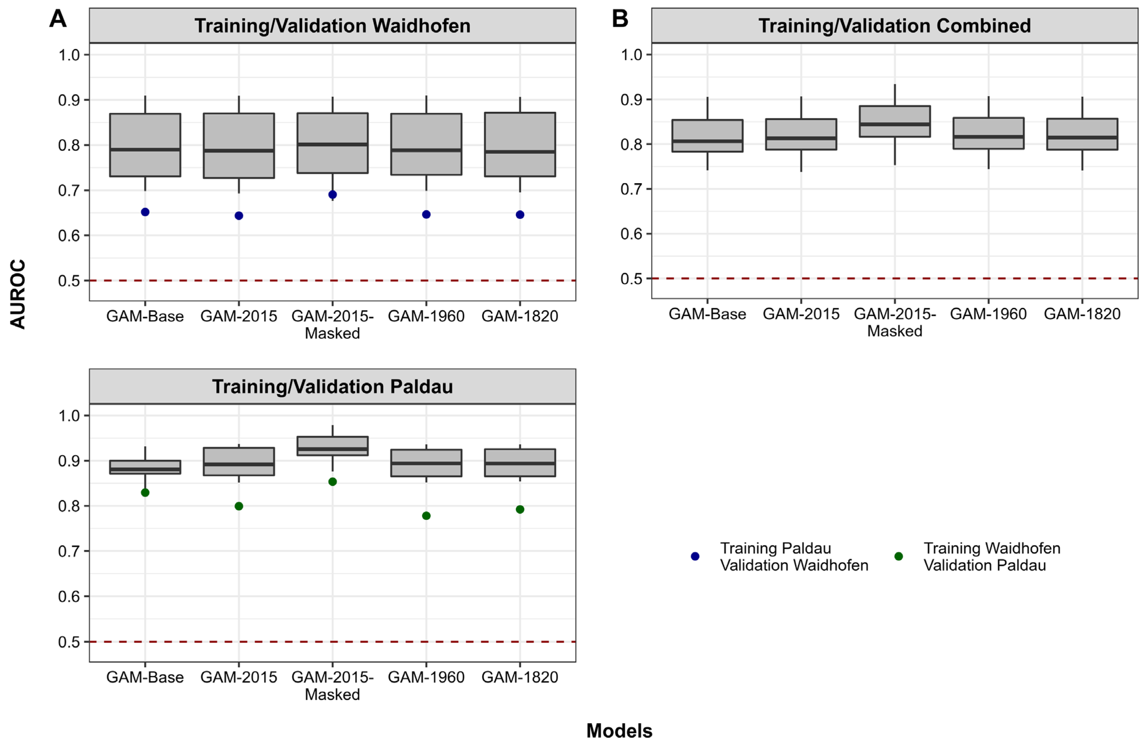
3.2.1. Model Performance and Transferability
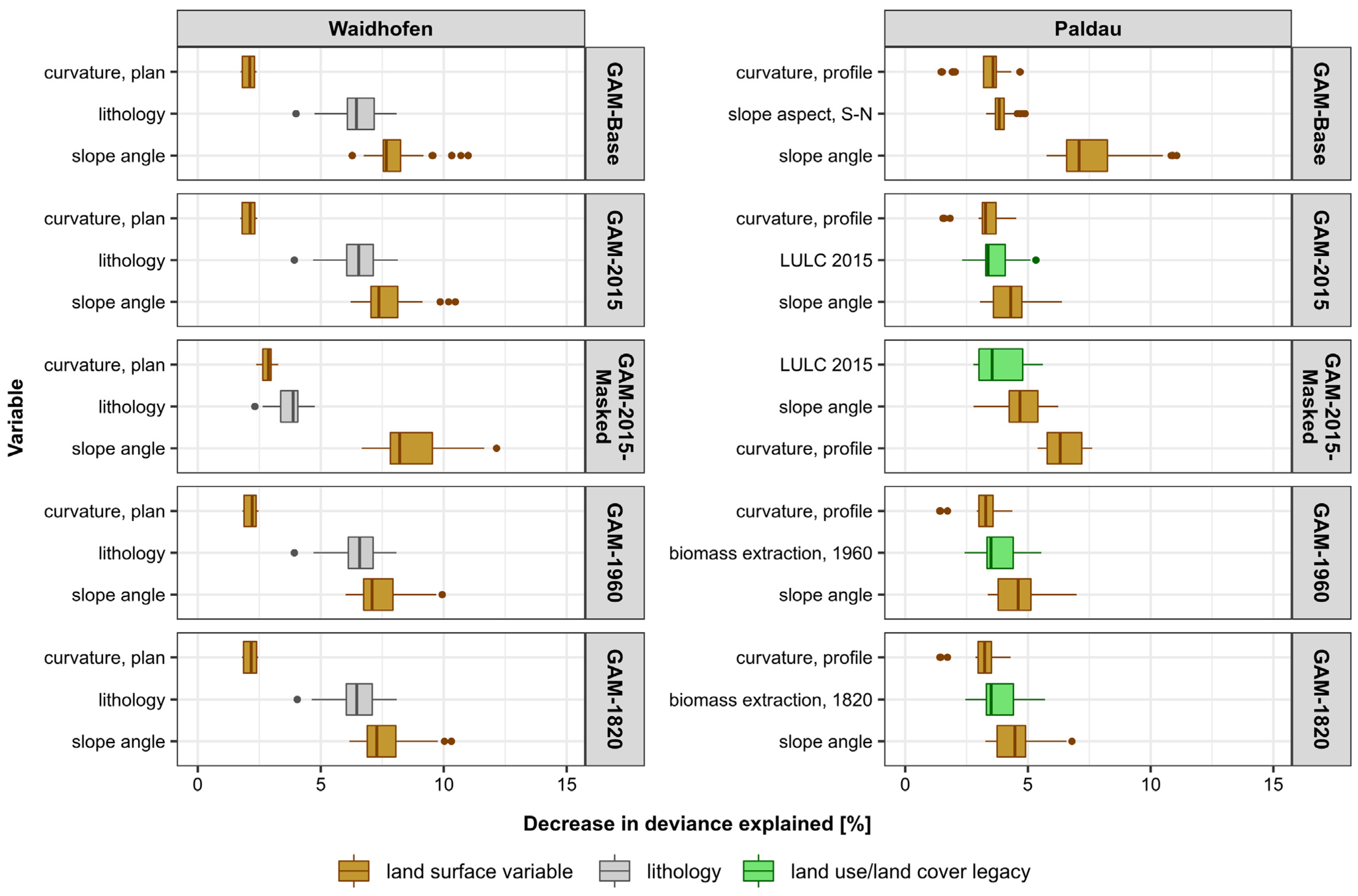
3.2.2. Variable Importance
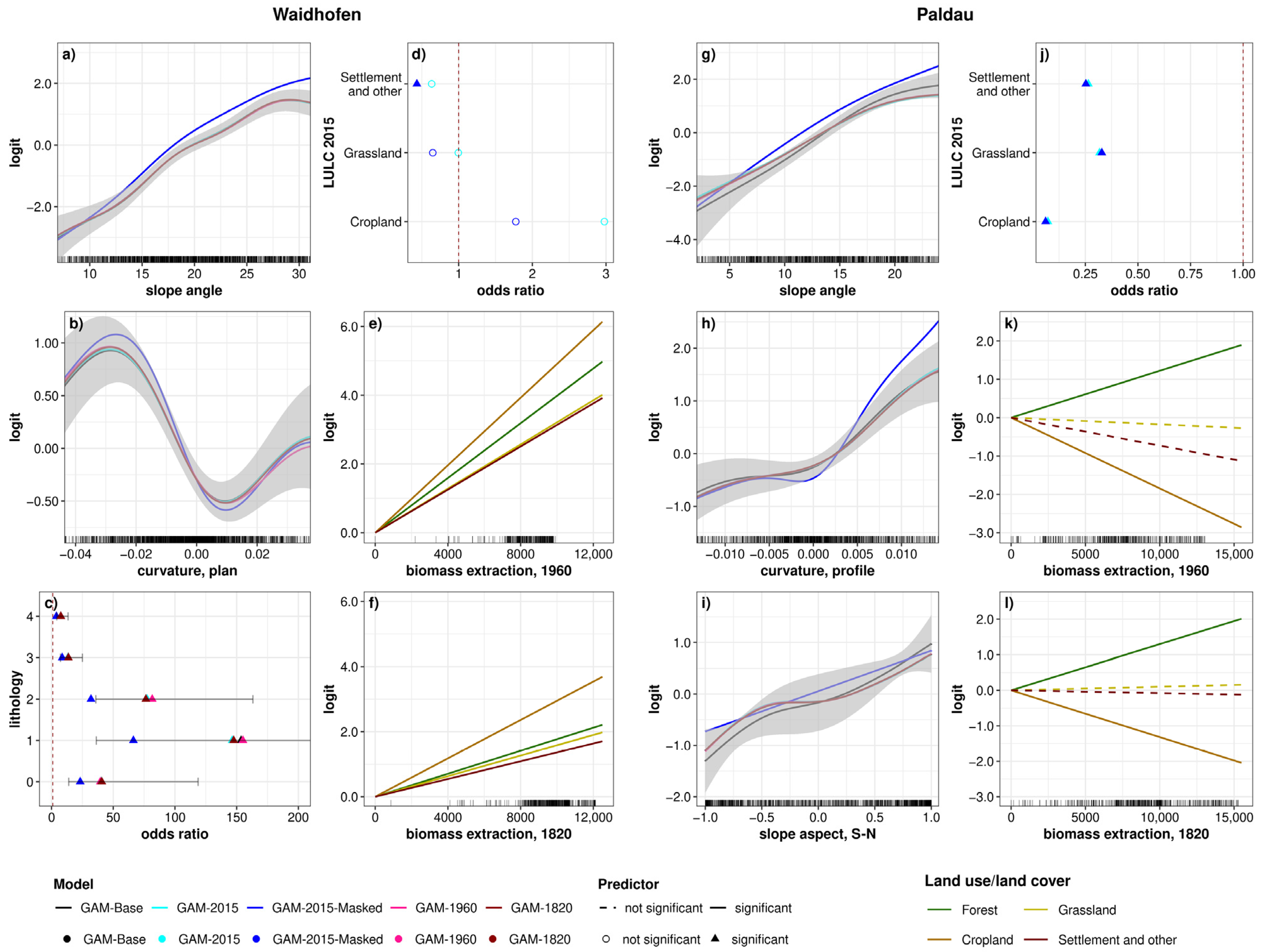
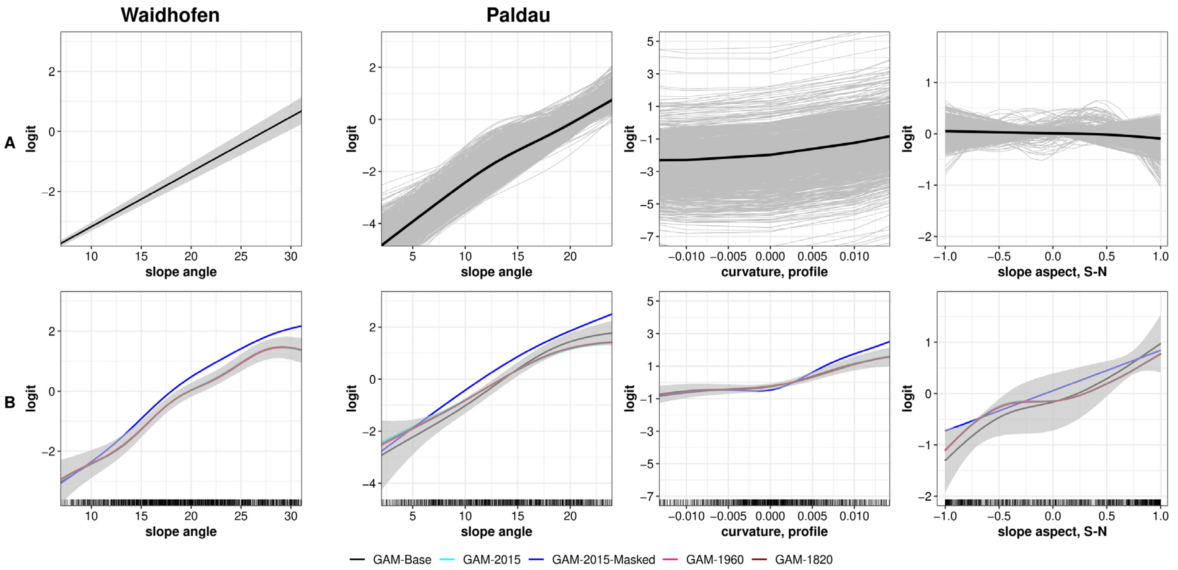
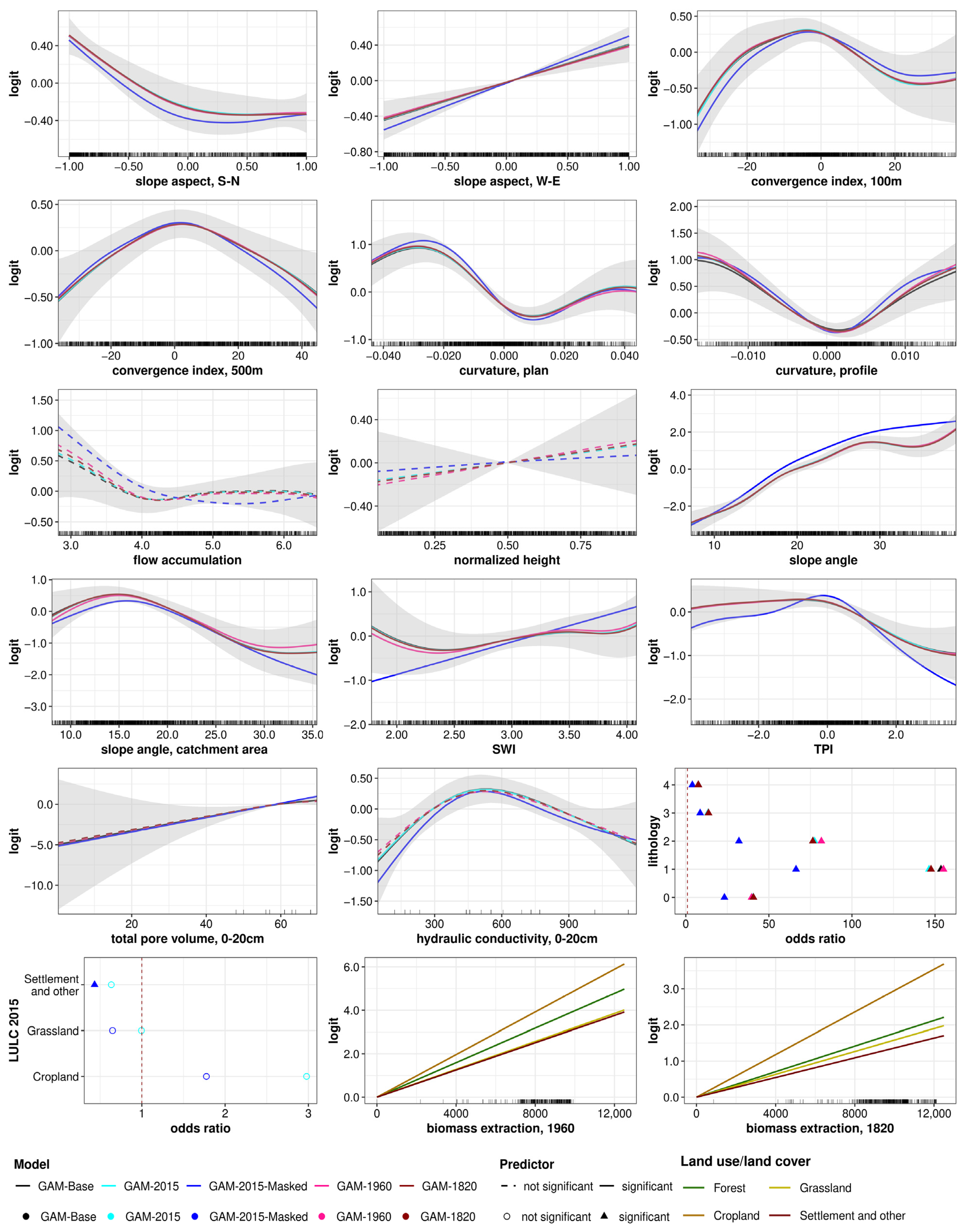
3.2.3. Predictor-Response Relationships
4. Discussion
4.1. Initial Objective: Effect of LULC Legacy on Modeling and Biases
4.2. Study Data: Challenges and Requirements
5. Conclusions and Outlook
Supplementary Materials
Author Contributions
Funding
Institutional Review Board Statement
Informed Consent Statement
Data Availability Statement
Acknowledgments
Conflicts of Interest
Appendix A. Descriptive Summary of Input Data

| Study Area | Source Holder | Resolution |
|---|---|---|
| airborne LiDAR-based high-resolution digital terrain model | ||
| Waidhofen | provincial government of Lower Austria | 1 m × 1 m, acquisition year: 2014 |
| Paldau | GIS department of the Styrian government | 1 m × 1 m, acquisition year: 2009 |
| hydrologic and hydropedologic parameters | ||
| Waidhofen | Austrian Research Centre for Forests | 50 m × 50 m, year: 2014 |
| Paldau | 100 m × 100 m, year 2017 | |
| geological basemaps | ||
| Waidhofen | Geological Survey of Austria | 1:50,000 |
| Paldau | GIS department of the Styrian government | 1:50,000 |
| land Use/Land Cover Category | Time Cut 1820 | Time Cut 2015 |
|---|---|---|
| LULC Types in the Franciscan Cadastre * | IACS, Orthophotos | |
| forest (including forest pasture) | Hardwood forests, Coniferous forests, Mixed forests, Chestnut forests, Meadows with fruit trees | All forest types digitized from orthophotos |
| grassland | Dry meadows, wet meadows, pastures, community pastures, shrubs | IACS agricultural parcel: Grassland, alpine pastures, pasture |
| cropland | Orchards, vegetable gardens, vineyards, arable land (with fruit trees, trees and vines) | IACS agricultural parcel: arable land |
| settlement and other | Marshes, lakes, ponds, rivers and streams, wastelands and bare rocks, buildings (all types), trails (all types) | Remaining area, which includes, e.g., buildings, impervious surfaces, water bodies, excavation pits and quarries, urban green, near-natural areas |

| Waidhofen | Paldau | ||||||
|---|---|---|---|---|---|---|---|
| Number | landslides | 621 | 418 | ||||
| scarps | 829 | 469 | |||||
| bodies | 663 | 348 | |||||
| samples | 974 | 559 | |||||
| Total Area [m2] (%) | landslides | 6,976,638 (5.31) | 1,621,250 (4.14) | ||||
| min | mean | max | min | mean | max | ||
| Area [m2] | landslides | 113 | 11,235 | 1,163,088 | 30 | 3879 | 206,842 |
| scarps | 2 | 517 | 79,640 | 12 | 140 | 1518 | |
| bodies | 52 | 9876 | 1,083,448 | 24 | 3949 | 206,842 | |
| Perimeter [m] | landslides | 44 | 451 | 7250 | 26 | 163 | 1821 |
| scarps | 7 | 101 | 3013 | 18 | 71 | 373 | |
| bodies | 29 | 297 | 4548 | 28 | 168 | 1821 | |
Appendix B. Summary of Model Assessment Results
| Model | Min | Max | IQR | Transfer | |
|---|---|---|---|---|---|
| A: Waidhofen | |||||
| GAM-Base | 0.79 | 0.7 | 0.91 | 0.14 | 0.65 |
| GAM-2015 | 0.79 | 0.69 | 0.91 | 0.14 | 0.64 |
| GAM-2015-Masked | 0.8 | 0.68 | 0.91 | 0.13 | 0.69 |
| GAM-1960 | 0.79 | 0.7 | 0.91 | 0.14 | 0.65 |
| GAM-1820 | 0.78 | 0.7 | 0.91 | 0.14 | 0.65 |
| B: Paldau | |||||
| GAM-Base | 0.88 | 0.83 | 0.93 | 0.03 | 0.83 |
| GAM-2015 | 0.89 | 0.85 | 0.94 | 0.06 | 0.8 |
| GAM-2015-Masked | 0.93 | 0.88 | 0.98 | 0.04 | 0.85 |
| GAM-1960 | 0.89 | 0.85 | 0.94 | 0.06 | 0.78 |
| GAM-1820 | 0.89 | 0.85 | 0.94 | 0.06 | 0.79 |
| C: Combined | |||||
| GAM-Base | 0.81 | 0.74 | 0.91 | 0.07 | |
| GAM-2015 | 0.81 | 0.74 | 0.91 | 0.07 | |
| GAM-2015-Masked | 0.84 | 0.75 | 0.93 | 0.07 | |
| GAM-1960 | 0.82 | 0.74 | 0.91 | 0.07 | |
| GAM-1820 | 0.81 | 0.74 | 0.91 | 0.07 | |
| Model | mAUROC | N * | Z | p-Values | |
|---|---|---|---|---|---|
| A: Waidhofen | |||||
| GAM-2015 | 0.79 | ||||
| <GAM-1820 | 0.78 | 36 | 2.7 | 0.01 | 0.45 |
| =GAM-Base | 0.79 | 35 | 0.93 | 0.18 | 0.16 |
| <GAM-1960 | 0.79 | 36 | 4.24 | <0.001 | 0.72 |
| <GAM-2015-Masked | 0.80 | 36 | 2.24 | 0.02 | 0.37 |
| B: Paldau | |||||
| GAM-Base | 0.88 | ||||
| <GAM-1960 | 0.89 | 66 | 5.01 | <0.001 | 0.62 |
| <GAM-1820 | 0.89 | 66 | 4.35 | <0.001 | 0.54 |
| =GAM-2015 | 0.89 | 66 | 1.54 | 0.06 | 0.19 |
| < GAM-2015-Masked | 0.93 | 66 | 7.03 | <0.001 | 0.87 |
| Variable | Study Area | GAM-Base | GAM-2015 | GAM-2015- Masked | GAM-1960 | GAM-1820 |
|---|---|---|---|---|---|---|
| land surface variable | ||||||
| convergence index, 100 m | Wh | 1.23 (5) | 1.27 (5) | 1.3 (6) | 1.15 (5) | 1.17 (5) |
| P | 0.91 (7) | 0.97 (8) | 0.71 (11) | 0.96 (8) | 0.98 (7) | |
| convergence index, 500 m | Wh | 0.87 (8) | 0.86 (9) | 0.99 (9) | 0.83 (10) | 0.86 (9) |
| P | 0.93 (6) | 1.16 (6) | 3.25 (4) | 1.2 (6) | 1.18 (6) | |
| curvature, plan | Wh | 2.09 (3) | 2.1 (3) | 2.83 (3) | 2.17 (3) | 2.17 (3) |
| P | 2.38 (4) | 1.43 (5) | 0.84 (10) | 1.46 (5) | 1.49 (5) | |
| curvature, profile | Wh | 1.45 (4) | 1.58 (4) | 1.78 (4) | 1.65 (4) | 1.57 (4) |
| P | 3.32 (3) | 3.2 (3) | 6.37 (1) | 3.08 (3) | 3.05 (3) | |
| flow accumulation | Wh | 0.42 (13) | 0.43 (12) | 0.48 (14) | 0.5 (13) | 0.46 (12) |
| P | 0.07 (15) | 0.2 (16) | 0.46 (13) | 0.22 (16) | 0.21 (16) | |
| normalized height | Wh | 0.02 (15) | 0.02 (16) | 0.05 (16) | 0.04 (16) | 0.03 (16) |
| P | 0.95 (5) | 0.95 (9) | 3.15 (5) | 0.93 (9) | 0.93 (9) | |
| slope angle | Wh | 8.01 (1) | 7.7 (1) | 8.63 (1) | 7.45 (1) | 7.61 (1) |
| P | 7.68 (1) | 4.38 (1) | 4.62 (2) | 4.77 (1) | 4.64 (1) | |
| slope angle, catchment area | Wh | 1.11 (7) | 1.15 (6) | 1.1 (8) | 1.07 (7) | 1.15 (6) |
| P | 0.55 (11) | 0.47 (12) | 0.2 (15) | 0.44 (12) | 0.43 (12) | |
| slope aspect, S-N | Wh | 1.12 (6) | 1.07 (7) | 1.11 (7) | 1.06 (8) | 1.12 (7) |
| P | 3.94 (2) | 2.3 (4) | 1.25 (8) | 2.36 (4) | 2.33 (4) | |
| slope aspect, W-E | Wh | 0.61 (11) | 0.58 (11) | 0.84 (10) | 0.52 (12) | 0.56 (11) |
| P | 0.32 (13) | 0.29 (14) | 1.68 (6) | 0.27 (15) | 0.27 (15) | |
| TPI | Wh | 0.86 (9) | 0.89 (8) | 1.64 (5) | 0.89 (9) | 0.91 (8) |
| P | 0.7 (9) | 0.84 (11) | 0.14 (16) | 0.84 (11) | 0.84 (11) | |
| SWI | Wh | 0.66 (10) | 0.66 (10) | 0.39 (15) | 0.68 (11) | 0.67 (10) |
| P | 0.66 (10) | 0.39 (13) | 0.95 (9) | 0.35 (13) | 0.35 (13) | |
| soil | ||||||
| total pore volume | Wh | 0.35 (14) | 0.31 (14) | 0.51 (13) | 0.29 (15) | 0.31 (15) |
| P | 0.47 (12) | 0.86 (10) | 0.68 (12) | 0.87 (10) | 0.87 (10) | |
| hydraulic conductivity | Wh | 0.44 (12) | 0.41 (13) | 0.62 (11) | 0.35 (14) | 0.38 (14) |
| P | 0.9 (8) | 0.98 (7) | 1.3 (7) | 0.98 (7) | 0.97 (8) | |
| lithology | ||||||
| lithology/geology | Wh | 6.38 (2) | 6.37 (2) | 3.72 (2) | 6.37 (2) | 6.34 (2) |
| P | 0.25 (14) | 0.27 (15) | 0.39 (14) | 0.27 (14) | 0.28 (14) | |
| land use/land cover legacy | ||||||
| LULC 2015 | Wh | 0.26 (15) | 0.6 (12) | |||
| P | 3.64 (2) | 3.92 (3) | ||||
| biomass extraction, 1960 * | Wh | 1.07 (6) | ||||
| P | 3.81 (2) | |||||
| biomass extraction, 1820 * | Wh | 0.43 (13) | ||||
| P | 3.85 (2) |


References
- Crozier, M.J.; Glade, T. Landslide Hazard and Risk: Issues, Concepts and Approach. In Landslide Hazard and Risk; Glade, T., Anderson, M., Crozier, M.J., Eds.; John Wiley & Sons: Chichester, UK, 2005; pp. 1–40. [Google Scholar]
- Gariano, S.L.; Guzzetti, F. Landslides in a changing climate. Earth-Sci. Rev. 2016, 162, 227–252. [Google Scholar] [CrossRef] [Green Version]
- Schweigl, J.; Hervás, J. Landslide Mapping in Austria; European Commission, Joint Research Centre: Luxembourg; Ispra, Italy, 2009. [Google Scholar] [CrossRef]
- Reichenbach, P.; Busca, C.; Mondini, A.C.; Rossi, M. The Influence of Land Use Change on Landslide Susceptibility Zonation: The Briga Catchment Test Site (Messina, Italy). Environ. Manag. 2014, 54, 1372–1384. [Google Scholar] [CrossRef] [PubMed] [Green Version]
- Papathoma-Köhle, M.; Glade, T. The role of vegetation cover change for landslide hazard and risk. In The Role of Ecosystems in Disaster Risk Reduction; UNU-Press: Tokyo, Japan, 2013; pp. 293–320. [Google Scholar]
- Brenning, A.; Schwinn, M.; Ruiz-Páez, A.P.; Muenchow, J. Landslide susceptibility near highways is increased by 1 order of magnitude in the Andes of southern Ecuador, Loja province. Nat. Hazards Earth Syst. Sci. 2015, 15, 45–57. [Google Scholar] [CrossRef] [Green Version]
- Goetz, J.; Guthrie, R.H.; Brenning, A. Forest harvesting is associated with increased landslide activity during an extreme rainstorm on Vancouver Island, Canada. Nat. Hazards Earth Syst. Sci. 2015, 15, 1311–1330. [Google Scholar] [CrossRef] [Green Version]
- van Westen, C.J.; Castellanos, E.; Kuriakose, S.L. Spatial data for landslide susceptibility, hazard, and vulnerability assessment: An overview. Eng. Geol. 2008, 102, 112–131. [Google Scholar] [CrossRef]
- Beguería, S. Changes in land cover and shallow landslide activity: A case study in the Spanish Pyrenees. Geomorphology 2006, 74, 196–206. [Google Scholar] [CrossRef] [Green Version]
- Gariano, S.L.; Petrucci, O.; Rianna, G.; Santini, M.; Guzzetti, F. Impacts of past and future land changes on landslides in southern Italy. Reg. Environ. Chang. 2018, 18, 437–449. [Google Scholar] [CrossRef]
- Persichillo, M.G.; Bordoni, M.; Meisina, C. The role of land use changes in the distribution of shallow landslides. Sci. Total Environ. 2017, 574, 924–937. [Google Scholar] [CrossRef] [PubMed]
- Pisano, L.; Zumpano, V.; Malek, Ž.; Rosskopf, C.M.; Parise, M. Variations in the susceptibility to landslides, as a consequence of land cover changes: A look to the past, and another towards the future. Sci. Total Environ. 2017, 601–602, 1147–1159. [Google Scholar] [CrossRef]
- Lopez-Saez, J.; Corona, C.; Eckert, N.; Stoffel, M.; Bourrier, F.; Berger, F. Impacts of land-use and land-cover changes on rockfall propagation: Insights from the Grenoble conurbation. Sci. Total Environ. 2016, 547, 345–355. [Google Scholar] [CrossRef]
- Cuddington, K. Legacy Effects: The Persistent Impact of Ecological Interactions. Biol. Theory 2011, 6, 203–210. [Google Scholar] [CrossRef]
- Foster, D.; Swanson, F.; Aber, J.; Burke, I.; Brokaw, N.; Tilman, D.; Knapp, A. The Importance of Land-Use Legacies to Ecology and Conservation. BioScience 2003, 53, 77–88. [Google Scholar] [CrossRef] [Green Version]
- Munteanu, C.; Kuemmerle, T.; Keuler, N.S.; Müller, D.; Balázs, P.; Dobosz, M.; Griffiths, P.; Halada, L.; Kaim, D.; Király, G.; et al. Legacies of 19th century land use shape contemporary forest cover. Glob. Environ. Chang. 2015, 34, 83–94. [Google Scholar] [CrossRef]
- Kuussaari, M.; Bommarco, R.; Heikkinen, R.K.; Helm, A.; Krauss, J.; Lindborg, R.; Öckinger, E.; Pärtel, M.; Pino, J.; Rodà, F.; et al. Extinction debt: A challenge for biodiversity conservation. Trends Ecol. Evol. 2009, 24, 564–571. [Google Scholar] [CrossRef]
- Perring, M.P.; Frenne, P.D.; Baeten, L.; Maes, S.L.; Depauw, L.; Blondeel, H.; Carón, M.M.; Verheyen, K. Global environmental change effects on ecosystems: The importance of land-use legacies. Glob. Chang. Biol. 2016, 22, 1361–1371. [Google Scholar] [CrossRef]
- Sonny Digital LiDAR-Terrain Models of Austria (last change 02 March 2021 16:01:16) 2016. Available online: https://data.opendataportal.at/dataset/dtm-austria (accessed on 30 June 2021).
- Haugerud, R.; Harding, D.; Johnson, S.; Harless, J.; Weaver, C.; Sherrod, B. High-Resolution Lidar Topography of the Puget Lowland, Washington —A Bonanza for Earth Science. GSA Today 2003, 13. [Google Scholar] [CrossRef]
- Petschko, H.; Bell, R.; Glade, T. Effectiveness of visually analyzing LiDAR DTM derivatives for earth and debris slide inventory mapping for statistical susceptibility modeling. Landslides 2016, 13, 857–872. [Google Scholar] [CrossRef]
- Schulz, W.H. Landslides mapped using LIDAR imagery, Seattle, Washington. US Geol. Surv. Open-File Rep. 2004, 1396. [Google Scholar] [CrossRef]
- Eeckhaut, M.V.D.; Poesen, J.; Verstraeten, G.; Vanacker, V.; Nyssen, J.; Moeyersons, J.; Beek, L.P.H.v.; Vandekerckhove, L. Use of LIDAR-derived images for mapping old landslides under forest. Earth Surf. Process. Landf. 2007, 32, 754–769. [Google Scholar] [CrossRef]
- Malamud, B.D.; Turcotte, D.L.; Guzzetti, F.; Reichenbach, P. Landslide inventories and their statistical properties. Earth Surf. Process. Landf. 2004, 29, 687–711. [Google Scholar] [CrossRef]
- Stanley, T.A.; Kirschbaum, D.B. Effects of inventory bias on landslide susceptibility calculations. In Proceedings of the Landslides: Putting Experience, Knowledge and Emerging Technologies into Practice; Association of Environmental & Engineering Geologists (AEG), Roanoke, VA, USA, 4–8 June 2017; pp. 794–806. [Google Scholar]
- Steger, S.; Brenning, A.; Bell, R.; Glade, T. The influence of systematically incomplete shallow landslide inventories on statistical susceptibility models and suggestions for improvements. Landslides 2017, 14, 1767–1781. [Google Scholar] [CrossRef] [Green Version]
- Petschko, H.; Bell, R.; Glade, T. Relative Age Estimation at Landslide Mapping on LiDAR Derivatives: Revealing the Applicability of Land Cover Data in Statistical Susceptibility Modelling. In Landslide Science for a Safer Geoenvironment; Springer Nature: Cham, Switzerland, 2014; pp. 337–343. [Google Scholar]
- Bell, R.; Petschko, H.; Röhrs, M.; Dix, A. Assessment of landslide age, landslide persistence and human impact using airborne laser scanning digital terrain models. Geogr. Ann. Ser. A Phys. Geogr. 2012, 94, 135–156. [Google Scholar] [CrossRef]
- van Westen, C.J.; van Asch, T.W.J.; Soeters, R. Landslide hazard and risk zonation—why is it still so difficult? Bull. Eng. Geol. Environ. 2006, 65, 167–184. [Google Scholar] [CrossRef]
- STATISTIK AUSTRIA Ein Blick auf die Gemeinde Waidhofen an der Ybbs (30301). Österreich Besser Verstehen. Bevölkerungsentwicklung 1869–2019 [A Look at the Municipality of Waidhofen an der Ybbs (30301). Understanding Austria Better. Population Development 1869–2019] 2011. Available online: https://www.statistik.at/blickgem/G0201/g30301.pdf (accessed on 30 June 2021).
- Wessely, G. Geologie der Österreichischen Bundesländer-Niederösterreich [Geology of the Austrian Federal Provinces-Lower Austria]; Verlag der Geologischen Bundesanstalt: Wien, Österreich, 2006. [Google Scholar]
- Gross, M. Beitrag zur Lithostratigraphie des Oststeirischen Beckens (Neogen/Pannonium; Österreich). In Stratigraphia Austriaca; Piller, W.E., Ed.; Schriftenreihe der Erdwissenschaftlichen Kommissionen/Österreichische Akademie der Wissenschaften; Österreichische Akademie der Wissenschaften: Wien, Austria, 2003; pp. 11–62. [Google Scholar]
- STATISTIK AUSTRIA Ein Blick auf die Gemeinde Paldau (62384). Österreich Besser Verstehen. Bevölkerungsentwicklung 1869 —2019 [A Look at the Municipality of Paldau (62384). Understanding Austria Better. Population Development 1869—2019] 2011. Available online: https://www.statistik.at/blickgem/G0201/g62384.pdf (accessed on 30 June 2021).
- Bell, R.; Glade, T.; Granica, K.; Heiss, G.; Leopold, P.; Petschko, H.; Pomaroli, G.; Proske, H.; Schweigl, J. Landslide Susceptibility Maps for Spatial Planning in Lower Austria. In Landslide Science and Practice. Volume 1: Landslide Inventory and Susceptibility and Hazard Zoning; Margottini, C., Canuti, P., Sassa, K., Eds.; Springer: Berlin/Heidelberg, Germany, 2013; pp. 467–472. [Google Scholar]
- Proske, H.; Bauer, C. Methodik zur Erstellung einer Gefahrenhinweiskarte für Rutschungen in der Steiermark [Methodology of the generation of an indicative hazard map for landslides in Styria]. Torrent Avalanche Landslide Rock Fall 2015, 175, 84–95. [Google Scholar]
- Schwenk, H.; Spendlingwimmer, R.; Salzer, F. Massenbewegungen in Niederösterreich 1953—1990 [Mass Movements in Lower Austria 1953—1990]. Jahrb. Der Geol. Bundesanst. 1992, 132, 597–660. [Google Scholar]
- Hornich, R.; Adelwöhrer, R. Landslides in Styria in 2009. Geomech. Tunn. 2010, 3, 455–461. [Google Scholar] [CrossRef]
- Lemenkova, P.; Glade, T.; Promper, C. Economic Assessment of Landslide Risk for the Waidhofen a.d. Ybbs Region, Alpine Foreland, Lower Austria. Protecting Society through Improved Understanding. In Proceedings of the 11th International Symposium on Landslides and the 2nd NorthAmerican Symposium on Landslides and Engineered Slopes, Banff, AB, Canada, 2–8 June 2012; pp. 279–285. [Google Scholar] [CrossRef]
- Eder, A.; Sotier, B.; Klebinder, K.; Sturmlechner, R.; Dorner, J.; Markat, G.; Schmid, G.; Strauss, P. Hydrologische Bodenkenndaten der Böden Niederösterreichs (HydroBodNÖ) [Data on Hydrological Soil Characteristics of Soils in Lower Austria]; Bundesamt für Wasserwirtschaft, Institut für Kulturtechnik und Bodenwasserhaushalt; Bundesforschungszentrum für Wald, Institut für Naturgefahren: Innsbruck, Austria, 2011. [Google Scholar]
- Klebinder, K.; Sotier, B.; Lechner, V.; Strauss, P. Hydrologische und Hydropedologische Kenndaten. Raabgebiet und Region. Südoststeiermark [Hydrologic and Hydropedologic Characteristics. Region. of Raab and Southeast. Styria]; Bundesforschungszentrum für Wald, Bundesamt für Wasserwirtschaft: Innsbruck, Austria, 2017; p. 30. Available online: https://wegenernet.org/downloads/Klebinder-etal_HydroBod-SOStmk-Projbericht_Jul2017.pdf (accessed on 30 June 2021).
- Bender, O. Analyse der Kulturlandschaftsentwicklung der Nördlichen Fränkischen Alb Anhand Eines Katasterbasierten Geoinformationssystems [Analysis of the Cultural Landscape Change of the Northern Franconian Alb Using a Cadastre-Based Geoinformation System]; Forschungen zur Deutschen Landeskunde; Deutsche Akademie für Landeskunde: Leipzig, Germany, 2007. [Google Scholar]
- Sandgruber, R. Österreichische Agrarstatistik 1750—1918; Hoffmann, A., Matis, H., Eds.; Wirtschafts- und Sozialstatistik Österreich-Ungarns; Verlag für Geschichte und Politik: Wien, Austria, 1978. [Google Scholar]
- Gingrich, S.; Erb, K.-H.; Krausmann, F.; Gaube, V.; Haberl, H. Long-term dynamics of terrestrial carbon stocks in Austria: A comprehensive assessment of the time period from 1830 to 2000. Reg. Environ. Chang. 2007, 7, 37–47. [Google Scholar] [CrossRef]
- Weiss, P.; Schieler, K.; Schadauer, K.; Englisch, M. Die Kohlenstoffbilanz des Österreichischen Waldes und Betrachtungen Zum Kyoto-Protokoll; Monographien; Umweltbundesamt: Wien, Austria, 2000. [Google Scholar]
- Knevels, R.; Brenning, A.; Gingrich, S.; Gruber, E.; Lechner, T.; Leopold, P.; Petschko, H.; Plutzar, C. Kulturlandschaft im Wandel: Ein indikatorenbasierter Rückblick bis in das 19. Jahrhundert. Fallstudie anhand der Gemeinden Waidhofen/Ybbs und Paldau [Cultural Landscape Change: An Indicator-Based Retrospect into the 19th Century. Case Study of the Municipalities Waidhofen/Ybbs and Paldau]. Mitt. Der Osterreichischen Geogr. Ges. 2021, 162, 255–285. [Google Scholar] [CrossRef]
- Erb, K.-H.; Haberl, H.; Jepsen, M.R.; Kuemmerle, T.; Lindner, M.; Müller, D.; Verburg, P.H.; Reenberg, A. A conceptual framework for analysing and measuring land-use intensity. Curr. Opin. Environ. Sustain. 2013, 5, 464–470. [Google Scholar] [CrossRef] [Green Version]
- Mayer, A.; Haas, W.; Wiedenhofer, D. How Countries’ Resource Use History Matters for Human Well-being—An Investigation of Global Patterns in Cumulative Material Flows from 1950 to 2010. Ecol. Econ. 2017, 134, 1–10. [Google Scholar] [CrossRef]
- Matthews, H.D.; Zickfeld, K.; Knutti, R.; Allen, M.R. Focus on cumulative emissions, global carbon budgets and the implications for climate mitigation targets. Environ. Res. Lett. 2018, 13, 010201. [Google Scholar] [CrossRef]
- Lechner, T.; Plutzar, C.; Knevels, R.; Gingrich, S. Long-Term Spatially Explicit Information on Land Use 1830–1960–2015: Case Study of the Municipalities Waidhofen/Ybbs and Paldau, Austria [Data set] 2021. 1.0.0. Available online: https://doi.org/10.5281/zenodo.4896571 (accessed on 30 June 2021).
- Cruden, D.M.; Varnes, D.J. Landslide Types and Processes. In Landslides Investigation and Mitigation. Transportation Research Board, US National Research Council; Turner, A.K., Schuster, R.L., Eds.; Special Report 247; U.S. National Academy of Sciences: Washington, DC, USA, 1996; pp. 36–75. [Google Scholar]
- Hussin, H.Y.; Zumpano, V.; Reichenbach, P.; Sterlacchini, S.; Micu, M.; van Westen, C.; Bălteanu, D. Different landslide sampling strategies in a grid-based bi-variate statistical susceptibility model. Geomorphology 2016, 253, 508–523. [Google Scholar] [CrossRef]
- Steger, S.; Glade, T. The Challenge of “Trivial Areas” in Statistical Landslide Susceptibility Modelling. In Proceedings of the Advancing Culture of Living with Landslides, Ljubljana, Slovenia, 29 May–2 June 2017; Mikos, M., Tiwari, B., Yin, Y., Sassa, K., Eds.; Springer International Publishing: Cham, Switzerland, 2017; pp. 803–808. [Google Scholar] [CrossRef]
- Hastie, T.; Tibshirani, R. Generalized Additive Models. Statist. Sci. 1986, 1, 297–310. [Google Scholar] [CrossRef]
- Wood, S.N. Generalized Additive Models: An Introduction with R, 2nd ed.; Chapman and Hall/CRC: Boca Raton, FL, USA, 2017. [Google Scholar]
- Brenning, A. Improved spatial analysis and prediction of landslide susceptibility: Practical recommendations. In Proceedings of the Landslides and Engineered Slopes: Protecting Society through Improved Understanding; Eberhardt, E., Froese, C., Turner, A.K., Leroueil, S., Eds.; CRC Press/Balkema: Banff, Canada, 2012; Volume 1, pp. 789–794. [Google Scholar]
- R Core Team. R: A Language and Environment for Statistical Computing, R version 3.5.2.; R Foundation for Statistical Computing: Vienna, Austria, 2018; Available online: https://www.R-project.org/ (accessed on 30 June 2021).
- Bischl, B.; Lang, M.; Kotthoff, L.; Schiffner, J.; Richter, J.; Studerus, E.; Casalicchio, G.; Jones, Z.M. mlr: Machine Learning in R. J. Mach. Learn. Res. 2016, 17, 1–5. [Google Scholar]
- Conrad, O.; Bechtel, B.; Dietrich, H.; Fischer, E.; Gerlitz, L.; Wehberg, J.; Wichmann, V.; Böhner, J. System for Automated Geoscientific Analyses (SAGA) v. 2.1.4. Geosci. Model. Dev. 2015, 8, 1991–2007. [Google Scholar] [CrossRef] [Green Version]
- Brenning, A.; Bangs, D.; Becker, M. RSAGA: SAGA Geoprocessing and Terrain Analysis; 2018. R Package Version 1.3.0. Available online: https://CRAN.R-project.org/package=RSAGA (accessed on 30 June 2021).
- Tarboton, D.G.; Dash, P.; Sazib, N. TauDEM 5.3: Guide to using the TauDEM command line functions 2015; Utah State University: Logan, UT, USA, 2015; Available online: http://hydrology.usu.edu/taudem/taudem5/TauDEM53CommandLineGuide.pdf (accessed on 30 June 2021).
- Koethe, R.; Lehmeier, F. SARA—System Zur Automatischen Relief-Analyse. User Manual, 2nd ed.; Department of Geography, University of Göttingen: Göttingen, Germany, 1996. [Google Scholar]
- Zevenbergen, L.W.; Thorne, C.R. Quantitative Analysis of Land Surface Topography. Earth Surf. Process. Landf. 1987, 12, 47–56. [Google Scholar] [CrossRef]
- Tarboton, D.G. A new method for the determination of flow directions and upslope areas in grid digital elevation models. Water Resour. Res. 1997, 33, 309–319. [Google Scholar] [CrossRef] [Green Version]
- Dietrich, H.; Böhner, J. Cold Air Production and Flow in a Low Mountain Range Landscape in Hessia. In SAGA–Seconds Out; Böhner, J., Blaschke, T., Montanarella, L., Eds.; Hamburger Beiträge zur Physischen Geographie und Landschaftsökologie; Universität Hamburg, Institut für Geographie: Hamburg, Germany, 2008; Volume 19, pp. 37–48. [Google Scholar]
- Böhner, J.; Selige, T. Spatial Prediction of Soil Attributes Using Terrain Analysis and Climate Regionalisation. Göttinger Geogr. Abh. 2006, 115, 13–27. [Google Scholar]
- Brenning, A.; Trombotto, D. Logistic regression modeling of rock glacier and glacier distribution: Topographic and climatic controls in the semi-arid Andes. Geomorphology 2006, 81, 141–154. [Google Scholar] [CrossRef]
- Guisan, A.; Weiss, S.B.; Weiss, A.D. GLM versus CCA spatial modeling of plant species distribution. Plant Ecol. 1999, 143, 107–122. [Google Scholar] [CrossRef]
- Hosmer, D.W.; Lemeshow, S.; Sturdivant, R.X. Wiley Series in Probability and Statistics. In Applied Logistic Regression; John Wiley & Sons: Hoboken, NJ, USA, 2013. [Google Scholar]
- Demšar, J. Statistical Comparisons of Classifiers over Multiple Data Sets. J. Mach. Learn. Res. 2006, 7, 1–30. [Google Scholar]
- Hothorn, T.; Hornik, K.; Wiel, M.A.v.d.; Zeileis, A. A Lego System for Conditional Inference. Am. Stat. 2006, 60, 257–263. [Google Scholar] [CrossRef] [Green Version]
- Benjamini, Y.; Hochberg, Y. Controlling the False Discovery Rate: A Practical and Powerful Approach to Multiple Testing. J. R. Stat. Society. Ser. B (Methodol.) 1995, 57, 289–300. [Google Scholar] [CrossRef]
- Goetz, J.; Brenning, A.; Marcer, M.; Bodin, X. Modeling the precision of structure-from-motion multi-view stereo digital elevation models from repeated close-range aerial surveys. Remote. Sens. Environ. 2018, 210, 208–216. [Google Scholar] [CrossRef]
- Knevels, R.; Petschko, H.; Proske, H.; Leopold, P.; Maraun, D.; Brenning, A. Event-Based Landslide Modeling in the Styrian Basin, Austria: Accounting for Time-Varying Rainfall and Land Cover. Geosciences 2020, 10, 217. [Google Scholar] [CrossRef]
- Steger, S.; Brenning, A.; Bell, R.; Glade, T. The propagation of inventory-based positional errors into statistical landslide susceptibility models. Nat. Hazards Earth Syst. Sci. 2016, 16, 2729–2745. [Google Scholar] [CrossRef] [Green Version]
- Szumilas, M. Explaining Odds Ratios. J. Can. Acad. Child Adolesc. Psychiatry 2010, 19, 227–229. [Google Scholar]
- Tasser, E.; Mader, M.; Tappeiner, U. Effects of land use in alpine grasslands on the probability of landslides. Basic Appl. Ecol. 2003, 4, 271–280. [Google Scholar] [CrossRef]
- Petschko, H.; Brenning, A.; Bell, R.; Goetz, J.; Glade, T. Assessing the quality of landslide susceptibility maps—Case study Lower Austria. Nat. Hazards Earth Syst. Sci. 2014, 14, 95–118. [Google Scholar] [CrossRef] [Green Version]
- Shirzadi, A.; Solaimani, K.; Roshan, M.H.; Kavian, A.; Chapi, K.; Shahabi, H.; Keesstra, S.; Ahmad, B.B.; Bui, D.T. Uncertainties of prediction accuracy in shallow landslide modeling: Sample size and raster resolution. CATENA 2019, 178, 172–188. [Google Scholar] [CrossRef]
- Biszak, E.; Biszak, S.; Timár, G.; Nagy, D.; Molnár, G. Historical topographic and cadastral maps of Europe in spotlight—Evolution of the MAPIRE web portal. In Proceedings of the 12th International Workshop on Digital Approaches to Cartographic Heritage, Venice, Italy, 26–28 April 2017; Volume 12, pp. 204–208. [Google Scholar]
- Gingrich, S.; Niedertscheider, M.; Kastner, T.; Haberl, H.; Cosor, G.; Krausmann, F.; Kuemmerle, T.; Müller, D.; Reith-Musel, A.; Jepsen, M.R.; et al. Exploring long-term trends in land use change and aboveground human appropriation of net primary production in nine European countries. Land Use Policy 2015, 47, 426–438. [Google Scholar] [CrossRef]
- Krausmann, F.; Gingrich, S.; Haberl, H.; Erb, K.-H.; Musel, A.; Kastner, T.; Kohlheb, N.; Niedertscheider, M.; Schwarzlmüller, E. Long-term trajectories of the human appropriation of net primary production: Lessons from six national case studies. Ecol. Econ. 2012, 77, 129–138. [Google Scholar] [CrossRef] [PubMed] [Green Version]
- Bätzing, W. Die Alpen—Tiefgreifende Nutzungsveränderungen als Herausforderung für den Naturschutz [The Alps—Profound changes in human uses present challenges to nature conservation]. Nat. Und Landsch. 2017, 92, 398–406. [Google Scholar] [CrossRef]


| Year | Study Area | Source | Source Holder | Q | Q-Explanation |
|---|---|---|---|---|---|
| Land use and land cover | |||||
| 1820 | Wh | Maps of Franciscan Cadastre | Provincial Archive of Lower Austria | ++ | Sharp delimitation of utilization unit |
| P | Federal Office for Calibration and Measurement | ++ | |||
| 1962 | Wh | Aerial images | Federal Office for Calibration and Measurement | ~ | Differentiation based on greyscale aerial photography |
| 1953 | P | ~ | |||
| 2015 | Wh, P | Orthophotos & IACS * | Open Data Austria | ++ | Parcel-sharp delimitation of arable land and grassland |
| Agricultural yields (cereal and grassland) | |||||
| 1820 | Wh | Text records of Franciscan Cadastre | Provincial Archive of Lower Austria | + | based on two cadastral municipalities of Waidhofen |
| 1820 | P | Sandgruber [42] | ~ | average of Styria | |
| 1960 | Wh, P | Agricultural statistics | Statistics Austria Library | ++ | data on municipality level |
| 2015 | Wh, P | IACS * | Open Data Austria | + | data of farms in municipality |
| Wood yields | |||||
| 1820 | Wh | Text records of Franciscan Cadastre | Provincial Archive of Lower Austria | + | based on two cadastral municipalities of Waidhofen |
| 1820 | P | Gingrich et al. [43] | ~ | average of Styria | |
| 1965 | Wh, P | Weiss et al. [44] | ~ | Austrian average | |
| 2015 | Wh, P | Forest inventory | Federal Forest Office | ~ | state averages |
| Variable(s) | Software | Setting | Method |
|---|---|---|---|
| land surface variable | |||
| convergence index (100 m, 500 m) | SAGA GIS | r = 100 m, 500 m | [61] |
| curvature (plan, profile) | SAGA GIS | [62] | |
| flow accumulation, D-Infinity | TauDEM | log-transformed | [63] |
| normalized height | SAGA GIS | w = 5; t = 2; e = 2 | [64] |
| slope angle | SAGA GIS | [62] | |
| slope angle, catchment area | SAGA GIS | [65] | |
| slope aspect (S-N, W-E) | SAGA GIS | cosine, sine transformed | [62,66] |
| topographic position index (TPI) | SAGA GIS | r = 500 m | [67] |
| topographic wetness index (SWI) | SAGA GIS | [65] | |
| soil | |||
| total pore volume | up to 20 cm depth, median | ||
| hydraulic conductivity | up to 20 cm depth, median | ||
| lithology | |||
| geology | * ref: Waidhofen (vii), Paldau (i) | ||
| land use/land cover legacy | |||
| LULC 2015 | ref: ‘Forest’ | ||
| biomass extraction (1820, 1960) | sum since 1820 and 1960 |
Publisher’s Note: MDPI stays neutral with regard to jurisdictional claims in published maps and institutional affiliations. |
© 2021 by the authors. Licensee MDPI, Basel, Switzerland. This article is an open access article distributed under the terms and conditions of the Creative Commons Attribution (CC BY) license (https://creativecommons.org/licenses/by/4.0/).
Share and Cite
Knevels, R.; Brenning, A.; Gingrich, S.; Heiss, G.; Lechner, T.; Leopold, P.; Plutzar, C.; Proske, H.; Petschko, H. Towards the Use of Land Use Legacies in Landslide Modeling: Current Challenges and Future Perspectives in an Austrian Case Study. Land 2021, 10, 954. https://doi.org/10.3390/land10090954
Knevels R, Brenning A, Gingrich S, Heiss G, Lechner T, Leopold P, Plutzar C, Proske H, Petschko H. Towards the Use of Land Use Legacies in Landslide Modeling: Current Challenges and Future Perspectives in an Austrian Case Study. Land. 2021; 10(9):954. https://doi.org/10.3390/land10090954
Chicago/Turabian StyleKnevels, Raphael, Alexander Brenning, Simone Gingrich, Gerhard Heiss, Theresia Lechner, Philip Leopold, Christoph Plutzar, Herwig Proske, and Helene Petschko. 2021. "Towards the Use of Land Use Legacies in Landslide Modeling: Current Challenges and Future Perspectives in an Austrian Case Study" Land 10, no. 9: 954. https://doi.org/10.3390/land10090954