


Abstract
High-resolution spectroscopic visible data were obtained with the Ultraviolet and Visible Echelle Spectrograph on the Very Large Telescope. Our goal was to analyze the data in an effort to detect the presence of sodium in the atmosphere of hot Jupiter exoplanet KELT-10b, as well as characterize the orbit of the planet via the Rossiter-McLaughlin effect. Eighty spectra were collected during a single transit of KELT-10b. After standard spectroscopic calibration using ESO-Reflex, the synthetic telluric modeling software molecfit was applied to remove terrestrial atmospheric effects, and to refine the wavelength calibration. Sodium is recognized by its characteristic absorption doublet located at 5895.924 and 5889.951 Å, which can be seen in the planet atmosphere transmission spectrum and through excess absorption during the transit. The radial velocity of the host star was analyzed by measuring the average shift of absorption features from spectrum to spectrum. Our results indicate a sodium detection in the planet transmission spectrum with a line contrast of 0.66% and 0.43% ± 0.09% for the sodium DII and DI lines, respectively. Excess absorption measurements agree to within one half combined standard deviation between the planet transmission spectrum (0.143% ± 0.020%, a 7σ detection) and during the time series (0.124% ± 0.034%, a 3.6σ detection) in a band 1.25 Å wide. The wavelength grid corrections provided by molecfit were insufficient to determine radial velocities and measure the Rossiter-McLaughlin effect.
Export citation and abstract BibTeX RIS

Original content from this work may be used under the terms of the Creative Commons Attribution 4.0 licence. Any further distribution of this work must maintain attribution to the author(s) and the title of the work, journal citation and DOI.
1. Introduction
The early stages of exoplanet discovery and orbital characterization are giving way to more detailed characterization of their chemistry and developmental histories. Spectroscopic observations of a planet's atmosphere during transit can reveal the composition, dynamical history, and greater context of the planet-star system.
Hot Jupiter exoplanets are gas giant planets akin to those of our own solar system, typically 0.8–1.5 RJup, except these bodies orbit their host stars <0.1 au. These planets were among the first to be detected and later characterized, and represent an important proving ground for scientific theory and technique alike. Considering an absence of this planet type in our solar system, their existence both challenges and informs theories on planetary formation and evolution. The relative observability of their atmospheresinflated as they are from their close proximity to the heat of their host starspresents the opportunity to test and develop instrumentation, calibration, and modeling techniques necessary to further test theory. The development of theory and honing of technique so far performed on hot Jupiter systems can be extrapolated to planets of all kinds, including Earth-size planets. The momentum of the field is gaining steadily in this direction in hopes of detecting a habitable (or inhabited) planet.
The field of exoplanet atmospheric characterization first bore fruit in 2002 by detecting atomic sodium in the atmosphere of hot Jupiter HD209458b (Charbonneau et al. 2002) via visible transmission spectroscopy from the Hubble Space Telescope. Six years later, ground-based observations detected sodium in a second planet, HD189733b (Redfield et al. 2008), and confirmed the space-based detection in HD209458b (Snellen et al. 2008). Since then, detection of atomic species like sodium and potassium, and molecular species like water vapor (e.g., Kreidberg et al. 2014) and carbon monoxide (e.g., Brogi et al. 2014), have occurred from space and ground-based observatories.
The range of chemical detection avails itself to early comparative analysis. Current instrumentation and methods, like high-resolution transmission spectroscopy, enable measurement of narrow wavelength regimes that are singularly informative and also provide pieces to the larger puzzle of exoplanet atmospheres. For example, a comparative study using transmission spectroscopy of ten hot Jupiters by Sing et al. (2016) presents a means of resolving the conundrum between cloud-blocked spectral features and low abundance by comparing discrete wavelength bands, or indices, in the optical and infrared. Specifically, Sing et al. (2016) compare the strength of molecular absorption in the midinfrared (3.0–5.0 microns) to scattering in the blue optical (0.3–0.57 microns) for one index, MIR molecular absorption to the near infrared (1.22–1.33 microns) for a second, and finally the amplitude of observed water vapor features in the near infrared to clear atmosphere models for a third. Comparing these indices reveals trends, for example, that hazes are indicated by higher near-infrared to midinfrared continuum strengths with low-amplitude water vapor features. With this information, a smaller investment of telescope time can be used to vet out planets that are cloudy and uninformative from those that are conducive for further study.
In this paper, we present the analysis of high-resolution optical transmission spectroscopy for the hot Jupiter KELT-10b taken with the Ultraviolet and Visible Echelle Spectrograph (UVES) on the Very Large Telescope (VLT) during transit on 2018 July 17. Specifically, we investigate the wavelength range containing the sodium doublet of the UVES "red arm" from approximately 5800–6800 Å. Section 2 discusses the discovery and initial characterization of KELT-10b. Section 3 describes the data acquired from UVES. Section 4 details the calibration and particularly the telluric corrections using molecfit as well as the methods used to detect sodium during transit. The results and interpretations are presented in Section 5 and we conclude in Section 6.
2. KELT-10b
KELT-10b is the first exoplanet discovered by the Kilodegree Extremely Little Telescope-South transit survey (Pepper et al. 2012). The physical parameters of the host star and planet are given in Table 1. At the time of discovery, KELT-10b was the third deepest transit (Tdep = 1.4 mmag) among bright (V < 11) stars in the southern hemisphere and was considered an ideal target for further atmospheric characterization (Kuhn et al. 2016).
Table 1. Adopted Physical and Orbital Parameters of KELT-10b and Host Star
| Parameter | Symbol | Value | Unit | Reference |
|---|---|---|---|---|
| Stellar radius | Rs | 1.209 ± 0.047 | solar radii | 1 |
| Stellar mass | Ms | 1.112 ± 0.061 | solar mass | 1 |
| Stellar temperature | T | 5948 ± 74 | K | 1 |
| V mag | V | 10.62 ± 0.06 | 1 | |
| Systemic velocity | γ | 31.61 ± 1.29 | km s−1 | 2 |
| Planet radius | Rp | 1.399 ± 0.069 | Jupiter radii | 1 |
| Planet mass | Mp | 0.679 ± 0.039 | Jupiter mass | 1 |
| RV semiamplitude | Kp | 80 ± 3.5 | m s−1 | 1 |
| Epoch of transit | T0 | 2457066.72 ± 0.00027 | BJDTDB | 1 |
| Duration of transit | Tdur | 3.744 ± 0.038 | hours | 1 |
| Orbital period | P | 4.1662739 ± 0.0000063 | days | 1 |
| Inclination | i | 88.61 ± 0.86 | degrees | 1 |
| Eccentricity | e | 0 ± 0 | 1 | |
| Semimajor axis | a | 0.0525 ± 0.00097 | au | 1 |
References. From NASA Exoplanet Archive: (1) Kuhn et al. (2016) (2) Gaia Collaboration et al. (2018).
Download table as: ASCIITypeset image
Virtually all of physical parameters used in this analysis come from the KELT-10b discovery paper; there is little published follow-up literature. Kuhn et al. (2016) note that the planet receives an estimated insolation of 0.817 ± 0.068×10⁹ erg s−1 cm−2 (or 580x the solar constant), which is approximately four times the empirical limit suggested by Demory & Seager (2011) above which hot Jupiters will exhibit increasing amounts of radius inflation. This inflation causes KELT-10b to be 40% larger in radius than Jupiter with only two thirds the mass. Kuhn et al. (2016) further note that the host star is expanding and transitioning into the red giant phase, causing the stars surface to approach the planets and further drive inflation. As a result, KELT-10b is likely spiraling in toward the host, and will not survive after the next 1 Gyr.
After the initial detection of the transit signal, the Nasmyth Adaptive Optics System Near-Infrared Imager and Spectrograph instrument on the VLT at the ESO Paranal observatory was used to image KELT-10b in one of many steps to eliminate false positive scenarios like blended eclipsing binaries. The imaging revealed a faint (ΔK = 9 ± 03) off-axis companion to KELT-10b at 1.1 ± 0 013 away, with a 0.073 solar mass, consistent with a very late M-dwarf star (Kuhn et al.2016). It remains unclear if this faint object is a true companion to KELT-10. However, statistical models of Galactic stellar distributions (Dhital et al. 2010) indicated a 0.86% probability of the alignment occurring by chance, thus strongly suggesting they are bound. See Figure 6 in Kuhn et al. (2016) for the AO image.
3. UVES Observations
High-resolution spectroscopy of KELT-10b was acquired during its 2018 July 17 transit using the UVES instrument at the VLT at the ESO Paranal observatory. The red arm of UVES obtained 80 spectra between 4800 and 11,000 Å at R ∼ 60,000. The timing of the observing run and the predicted transit of KELT-10b are given in Table A1. The transit ephemerides were generated using the NASA Exoplanet Archive (Akeson et al. 2013). Full coverage of the transit was expected, with 206-second exposures producing 46 in-transit spectra, and 34 out-of-transit spectra (11 preingress and 23 postegress). The designation of in transit and out of transit are defined by including the uncertainty in the timing of ingress and egress, which was 5 minutes before and after, respectively. We made use of the entire 80 spectra data set in the analysis. Observing conditions, including seeing, airmass, and predicted transit timing are presented in Figure 1. The seeing remains greater than the slit width for nearly the entire run, implying the slit has been homogeneously illuminated.
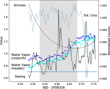
Figure 1. Variation of conditions during the observation period. The solid black line indicates airmass, the dotted line indicates normalized total count values, the dashed line indicates seeing per exposure, and the slit width (07) is indicated by the horizontal blue line. The light blue and dark blue markers are the normalized integrated water vapor noted in the FITS headers and the relative H2O columns measured by molecfit, respectively, and they are in good agreement.
Download figure:
Standard image High-resolution image4. Methods
4.1. Data Calibration
The raw data and calibration frames were downloaded from the ESO Archive and included: raw spectra from the red arm of the UVES instrument, bias, order definition, format check, flat, and ThAr lamp wavelength calibration frames, as well as a standard star frame taken once at the beginning of the evening. Data reduction was conducted using the UVES Workflow for Point Source Echelle Data version 5.10.4, in the Kepler-based ESO-Reflex software (Freudling et al. 2013). The output of the ESO-Reflex UVES workflow was a merged, 1D, wavelength-calibrated spectrum for each of the 80 spectra. Flux calibrated spectra are also produced in the UVES workflow but are not used in this study. The UVES red arm uses two CCDs: an upper and lower CCD designated U and L. The wavelength range of interest that contains the Na D sodium doublet falls on the U CCD from approximately 5800–6800 Å. Each spectrum was normalized by the mean flux value of that individual spectrum. Outliers for a given channel were removed according to a 3σ threshold around the mean flux value for that channel across all 80 spectra.
4.2. Telluric Removal via molecfit
The identification and removal of telluric features were done using software called molecfit. Molecfit uses atmospheric profile information including temperature, pressure, humidity, and molecular abundances in a line-by-line radiative transfer model to create a model telluric spectrum at resolutions up to 4,000,000 (Smette et al. 2015; Allart et al. 2017). The atmospheric profile is created by combining a standard profile and a Global Data Assimilation System profile; the former describes pressure, temperature, and molecular abundance by latitude and altitude; the latter is an NOAA generated profile that records pressure, temperature, humidity, and other meteorological data for a location every 3 hr. The model telluric spectrum is then fit to the continuum level, wavelength range, and instrumental resolution of the science spectra. In this way, the science spectra can be further wavelength calibrated to correct for instrumental shifts and imprecision in the initial wavelength solution, theoretically providing an "absolute" wavelength calibration. The dominant telluric features in the relevant wavelengths here are H2O and O2.
Molecfit fitting algorithms are optimized when discrete wavelength ranges are selected that contain well-defined telluric features, omit strong nontelluric absorption features (e.g., stellar), and are surrounded by relatively flat continuum. Molecfit fits the telluric abundances in these discrete sections and then extrapolates to model the features across the entire input spectrum. The initial molecfit fitting parameters for this project were adopted from Allart et al. (2017), who applied the software to correct HARPS spectra for the first time, which has a comparable wavelength range and resolution (although see Cauley et al. (2015) for a successful application of molecfit to HiRES data from Keck I).
The wavelength ranges and parameters were then iterated to balance fit quality and processing speed; the parameters used are presented in Table 2 and the wavelength ranges in Table A2. A full spectrum highlighting the wavelength ranges used is shown in Figure 2, and a closer look at the telluric features near 6280 Å before and after the telluric correction are presented in Figure 3. Although the wavelength region near 6280 Å is relatively far from the area of interest, this wavelength range is ideal to demonstrate the quality and method of the molecfit telluric removal, particularly the selection of discrete fit regions and the correction outside those regions. The output of molecfit are instrumental- and telluric-corrected spectra. The output wavelength is in nm and vacuum, which is then manually converted to air wavelengths in Angstroms using the equations of Ciddor (1996) implemented in the python astronomy suite PyAstronomy (Czesla et al. 2019).
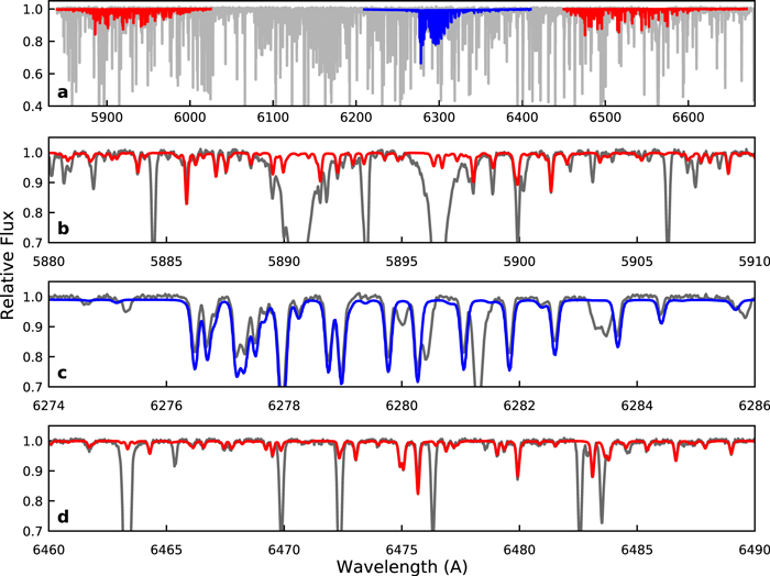
Figure 2. Normalized science spectrum overplotted with modeled telluric spectrum produced by molecfit. Panel (a) shows the full science and telluric spectrum with water vapor in red and oxygen in blue. Panels (b), (c), and (d) show specific regions in more detail where the quality of the telluric model can be directly compared to the uncorrected science spectrum.
Download figure:
Standard image High-resolution image
Figure 3. Closer look at the quality of molecfit telluric flux correction, highlighting airmass-dependent variability in telluric oxygen from 6277–6295 Å. Panel (a) shows the normalized uncorrected spectra plotted as a function of airmass, with the telluric model scaled by 50% and arbitrarily shifted. The green shaded regions are the discrete fit regions selected for the molecfit fitting procedure. Panel (b) shows the resulting corrected spectra, with the same discrete fit regions delineated by green dotted lines. Panels (c) and (d) show the fractional difference between individual and the mean uncorrected and corrected spectra, respectively.
Download figure:
Standard image High-resolution imageTable 2. Parameters for molecfit from Allart et al. (2017), and the for this Research
| Parameter | Value | Description | |
|---|---|---|---|
| Allart et al. (2017) | Current Project | ||
| Instrument | HARPS | UVES | |
| Ftol | 10−9 | 10−12 | χ convergence criteria |
| Xtol | 10−9 | 10−12 | Parameter convergence criteria |
| Molecules | H2O, O2 | H2O, O2 | Telluric molecules |
| Ncont | 3 | 3 | Degree of polynomial for continuum |
| a0 | 2000 | 1.1 | Constant offset for the continuum |
| nλ | 2 | 2 | Chebyschev degree for wavelength calibration |
| b0 | 0 | 0 | Constant Chebyschev for wavelength calibration |
| FWHM | 4.5 | 5.0 | FWHM of Gaussian profile in pixels |
| Kernel size | 15 | 30 | |
| Pixel scale | 0.16 | 0.18 | /pixel |
| Slit width | 1 | 0.7 | |
Download table as: ASCIITypeset image
The quality of telluric removal shown in Figure 3 appears notably high, as telluric oxygen and water vapor are reduced to the noise level of the spectrum. However, the quality of the "absolute" wavelength calibration was questionable and ultimately led to the biggest challenge of this analysis. The quality of the wavelength correction was not rendered suspect until attempts were made to measure the Rossiter-McLaughlin effect. See Section 4.6 for a discussion of the wavelength correction.
4.3. Barycentric and Radial Velocity Corrections
Next, a series of radial velocity Doppler shifts were performed. The barycentric velocity at the time of each observation was calculated via the python package barycorrpy (Kanodia & Wright 2018) and used to shift the spectra. Protocol for UVES defines the exposure time as the exposure start time, so the midpoint of each exposure is calculated as midpoint = start time + exposure time/2.
Next, the radial velocities of the star and planet, as well as the systemic velocity of the whole KELT-10 system, need to be accounted for. The radial velocities were calculated for the star and planet by assuming a circular orbit and the system parameters from Kuhn et al. (2016) listed in Table 1, and were found to vary from +0.014 to −0.018 km s−1 and −24.3 to +31.6 km s−1 for the star and planet, respectively. The stellar reflex motion corresponds to a wavelength shift of 0.0002 Å at 6000 Å, and is ignored in this analysis. On the other hand, the planet radial velocity corresponds to a shift of −/+ 0.33 Å at 6000 Å, and were applied in the present analysis following the method of, e.g., Wyttenbach et al. (2015) and Khalafinejad et al. (2017). See Section 4.4 for a more complete description.
The systemic velocity is taken into account by determining where the wavelength of the absorption feature of interest (here, sodium) would appear in the planet's atmosphere given the system's velocity. The KELT-10 systemic velocity is 31.61 ± 1.29 km s−1 (Gaia Collaboration et al. 2018), which redshifts the Na DI and DII lines ∼0.62 Å from 5895.924 and 5889.951 Å to 5896.546 and 5890.571 Å, respectively.
4.4. Planet Atmosphere Transmission Spectrum
As a planet transits its host star, the starlight passes through a ring, or annulus, of the planet's atmosphere, allowing the planet's atmospheric spectral information to be imprinted on the star's spectrum during the transit. The planet's atmospheric spectrum is extracted from this combined spectrum by comparing the depth of absorption features in transit to the depth of those features out of transit.
For our analysis, we follow the method described by Wyttenbach et al. (2015), who extract the planet spectrum by shifting the relative in-transit fluxes by the planet's radial velocity—which is blueshifted from ingress up to midtransit and redshifted from midtransit out to egress. The planet's radial velocity changes during transit from −16 to +16 km s−1 or ∼0.66 Å from ingress to egress.
The 80 spectra are separated into in-transit and out-of-transit bins based on the predicted transit ephemeris from the NASA Exoplanet Archive (Akeson et al. 2013); 37 and 43 spectra are in the in-transit and out-of-transit bins, respectively. The planet atmosphere transmission spectrum is extracted by first making a master out-of-transit spectrum (Fout) by coadding all of the individual spectra that occurred outside the predicted ingress and egress time, dividing each individual in-transit spectrum (f(λ,tin)) by this master out-of-transit spectrum, shifting the result by the planet's anticipated radial velocity at the midpoint of that exposure, and finally summing and normalizing the sum. Mathematically:

where S(λ) is the planet transmission spectrum. This final planet transmission spectrum theoretically preserves wavelength information and enables the detection of any atmosphere-specific phenomena, like high-speed winds, that would shift planetary atmospheric absorption features from their expected wavelengths. There are a variety of proposed atmospheric flow patterns that affect observed absorption features. A tidally locked hot Jupiter could experience an equatorial jetstream "superrotation," in which atmosphere heated on the dayside are driven to wind speeds faster than the planetary rotation rate (e.g., Showman & Polvani 2011). Similarly, a situation in which atmosphere is heated and upwells on the dayside and downwells as it cools on the nightside has been confirmed for HD 189733b (e.g., Flowers et al. 2019). The relevance of other important factors like vertical mixing (e.g., Komacek et al. 2019; Seidel et al. 2020a) can be extracted from this kind of atmospheric data, which overall improves our understanding of planets both extrasolar and local.
Relative depths are calculated by comparing the flux in a wavelength band centered on the feature, which should show a decrease in relative flux if present in the planet atmosphere, to two wavelength bands blueward and redward of the feature at the continuum level, which should show no change in relative flux during transit.
Common practice for atmospheric spectroscopy is to calculate the relative depth within a variety of bandwidths. This allows flexibility in cases where the position and line width of the absorption feature are uncertain (e.g., Snellen et al. 2008) or are expected to change over time compared to the stellar feature due to radial velocity changes. Typically, bandwidths on the order of 0.5–3.0 Å (or the velocity-scale equivalents) are used (e.g., Cauley et al. 2019; Casasayas-Barris et al. 2020). Further, larger bandwidths of 9 Å (e.g., Snellen et al. 2008), 20 Å (e.g., von Essen et al. 2020), and ranges from 15–90 Å (e.g., Nikolov et al. 2015) are applied when using or comparing high-resolution ground-based data to measurements from space-borne instruments like the Hubble and Spitzer Space Telescopes.
There is also a range of strategies regarding whether to define the reference bands and widths relative to the central band or absolutely. For example, Snellen et al. (2008) place the red and blue reference bands immediately adjacent to the central band and of the same width (i.e., if the central band is 1.0 Å wide then the blue and red bands are also 1.0 Å wide). In contrast, Wyttenbach et al. (2015) and Khalafinejad et al. (2017) define absolute reference bands: the former choosing a pair of 12 Å bands that are used for both DI and DII, the latter choosing two pairs of 1 Å bands, one for each Na D line. Charbonneau et al. (2002) chose a blend of relative and absolute: they defined an absolute wavelength range containing the sodium doublet and used the range modulo the central band as the reference bands.
The present research performed both the "relative" band method of Snellen et al. (2008) in which the reference bands are the same width as and immediately adjacent to the central band, and the "absolute" band method of Wyttenbach et al. (2015). When used, the absolute reference bands were 12.0 Å wide located in nearby relatively featureless parts of the continuum from 5870–5882 Å (B) and 5918–5930 Å (R).
At first, the central band (C) was centered on the expected Na D line positions in the systemic velocity reference frame (i.e., at the redshifted wavelengths expected from the KELT-10 systemic velocity). However, the final planet transmission spectrum yields bandcenters for the putative sodium features that are redshifted by 0.23 ± 0.06 Å compared to the expected position (see Section 5.1 for description and interpretation). Therefore, two iterations of the relative absorption depth measurement were performed: one defining the central bands according to the expected "fixed" position, and a second defining the central bands by performing a Gaussian fit to the features.
This strategy of defining the central band according to the expected "fixed" wavelength and fitting for the center wavelength was also applied in the later analysis of measuring the absorption depth via the spectrophotometric time series (see Section 4.5).
The relative depth was calculated by taking the mean flux in each band, averaging the reference bands and taking the difference. Mathematically:

In this calculation and all others, errors are propagated from the initial flux uncertainties produced by the ESO-Reflex data reduction combining Poisson errors and instrumental effects.
4.5. Spectrophotometric Time Series
A complementary method to that of Section 4.4 is to produce a time series of relative depth for an absorption feature, where the excess absorption caused by the planet's atmosphere is measured by its light curve. By this method, timing information is preserved, but specific wavelength information (e.g., excess blue or redshift) is lost. It is possible to bypass modeling the transit-like light curve for the specific feature and calculate the excess absorption by comparing the relative flux in and out of transit.
First, the relative flux is calculated in each individual stellar spectrum by comparing the flux in a central band to the flux in a blue and red band. Mathematically:

This is similar to the measurement in Equation (2), except that this is performed on each individual stellar spectrum instead of the atmospheric spectrum that is compared first to a master out-of-transit template. The same relative and absolute bands were applied to the time series depth calculation as that applied for the planet transmission spectrum in Section 4.4. The central band was also implemented in two ways. The first way was to fix the center of each line to its expected position in the systemic reference frame. The second way was to use the line center determined by Gaussian fitting of the Na DI and DII lines in each individual spectrum without implementing any correction for the radial velocity shift of the planet. The reasoning is that since specific wavelength information is lost in the final calculation, a more accurate determination of the change in flux can be obtained by ensuring the bands actually encompass the feature in question. Applying the planet's radial velocity shift correction to each spectrum is less important in this calculation for the same reason; the goal of doing so would be to align the spectra at the expected systemic position of the lines. However, as described in Section 4.4, the observed sodium features are redshifted 0.23 ± 0.06 Å from that expected position.
Wyttenbach et al. (2015), referencing Astudillo-Defru & Rojo (2013), defend the position that the absorption depth is well defined by taking the difference of averages between relative flux in transit to out of transit. That method is applied here:

Altogether, the relative absorption depth was calculated four ways for both the planet transmission spectrum and the time series: using either "relative" or "absolute" reference bands and either "fixed" or "fit" central bands. A range of bandwidths from 0.10 up to 5.0 Å were used.
4.6. Rossiter-McLaughlin Effect
The Rossiter-McLaughlin effect for transiting exoplanets is an anomaly in the observed radial velocity that the planet induces on the Doppler reflex motion of the host star (Winn 2011). As a planet begins transiting the stellar disk, a portion of the stellar rotation will be blocked and cause the radial velocity to be offset in the opposite sense. Put another way, as a planet transits the stellar disk, the planet traces a path of projected stellar rotation velocities and produces an enhancement in flux at those velocities (Hoeijmakers et al. 2018). In an idealized case if an exoplanet's orbit is aligned with the direction of stellar rotation, then a portion of the blueshifted hemisphere of the star (i.e., the hemisphere rotating toward the observer) is blocked during ingress and into the transit, and induces an excess redshift in the observed radial velocity (see Triaud's review in Deeg & Belmonte 2018; Gaudi & Winn 2007). As the planet continues the transit, it moves to block a portion of the star's redshifted hemisphere and induces an excess blueshift.
The magnitude of the excess Doppler shift and the particular shape of the affected radial velocity curve are determined by the particulars of the spin–orbit alignment between star and exoplanet, the transit impact parameter, the rotational speed of the star, and the planet-to-star size ratio. Therefore, extracting these astrophysical parameters is possible by modeling the radial velocity curve during an exoplanet transit (e.g., Ohta et al. 2005). A typical hot Jupiter produces a radial velocity change with semiamplitude on the order of 20 m s−1 (Triaud's review in Deeg & Belmonte 2018).
A first pass at measuring the Rossiter-McLaughlin effect began by extracting the radial velocity from spectra observed during the transit of KELT-10b. For spectra collected with UVES, the radial velocity of the target is not automatically generated and embedded in the FITS files, therefore the radial velocity needed to be extracted from each spectrum. In each spectrum, the line positions of suitable absorption features are determined using Gaussian fitting and then compared to their position in some reference spectrum—in this case, the spectrum closest to midtransit. The differences in each spectrum are averaged to determine the radial velocity for that spectrum, and finally plotted as a time series and modeled for the Rossiter-McLaughlin effect. For n absorption features in a spectrum at time t, the radial velocity vr is:

where λn,t is the position of line n in the spectrum at time t, and λn,mid is the midtransit reference spectrum.
Significant effort was invested into measuring the radial velocity shifts to eventually model the Rossiter-McLaughlin effect, but unfortunately this first pass was unsuccessful. Ultimately, we suspect that molecfit was unable to fully/precisely fine-tune the wavelength grid and correct for the instrumental effects introduced by the slit spectrograph of UVES. See Section 4.6.
5. Results and Discussion
5.1. KELT-10b Transmission Spectrum
We binned this final spectrum by 20 pixels (0.2 Å) and fit each Na DI and DII line with a simple Gaussian centered on the expected wavelengths of the sodium lines in the planet's reference frame (i.e., the wavelength's shifted to the systemic velocity of the KELT-10 system). The result is shown in Figure 4, with the reference wavelength denoted by the red-dashed line. We measure line a contrast of 0.66% and 0.43% ± .09% in the binned spectrum for the DII an DI lines, respectively, using for the error the standard deviation of the residuals. However, a visual inspection of the final transmission spectrum reveals significant scatter around the putative sodium lines and therefore strains credibility for a bona fide detection.
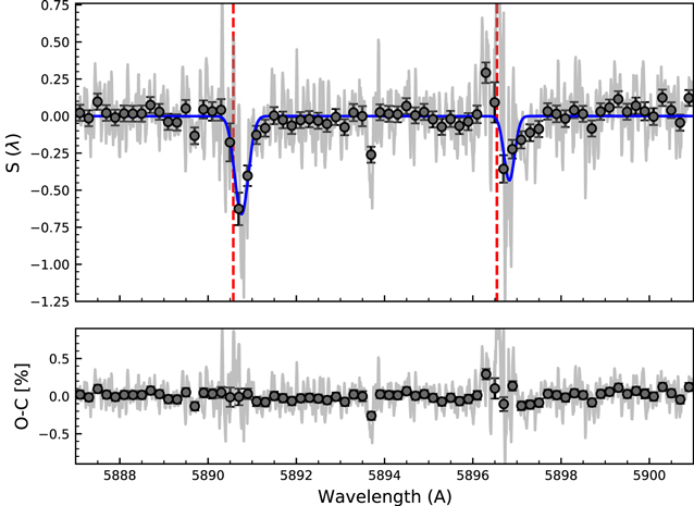
Figure 4. Planet atmosphere transmission spectrum of KELT-10b from 5887–5901 Å, in percent. Dark gray circles represent the data binned by 20 pixels or 0.2 Å, blue line is the Gaussian fit of the binned doublet flux, and red-dashed lines are expected line positions in the planet's reference frame. The actual line centers are redshifted by 0.23 ± 0.06 Å, or 12 ± 3 km s−1.
Download figure:
Standard image High-resolution imageThe measured line centers differ from the expected values for the planet reference wavelength by 0.23 ± 0.06 Å, averaging the shift of the two lines. Errors were propagated from the systemic redshift (31.69 ± 1.29 km s−1, or 0.623 ±0.018 Å) and extracted from the standard deviation of the Gaussian line fit residuals. Once again, the qualitative nature of the final transmission spectrum renders the significance of this redshift suspect. If astrophysical in nature, the redshift corresponds to 12 ± 3 km s−1 and is difficult to interpret. Blueshift in atmospheric transmission spectra have been detected previously (Redfield et al. 2008; Snellen et al. 2008; Wyttenbach et al. 2015) of the same magnitude presented here. Those shifts are interpreted as high-speed winds in the upper atmospheres of hot Jupiters blowing toward the observer as hot air from the tidally locked dayside of the planet circulates to the nightside. In the present case, a redshift is much harder to account for astrophysically. The interpretation is therefore that this is not a real phenomena, but instead an artifact introduced by the obfuscated combination of UVES instrumental shifts and molecfit wavelength correction.
5.2. Excess Absorption Depths
The relative excess absorption depth in the planet transmission spectrum and the time series of the sodium doublet were calculated using four different strategies for defining the centers and reference bandwidths: with a fixed and fit center, and an absolute and relative reference band. The results for all of these calculations are presented appendix Tables A3 and A4. The highest signal-to-noise ratio (S/N) with consistent values between the relative absorption depth and time series calculations was achieved using absolute reference bands, fit centers, and a bandwidth of 1.25 Å. Excess absorption depths of 0.143% ± 0.020% (7σ) and 0.124% ± 0.034% (3.6σ) were measured for the planet transmission spectrum and time series, respectively. The excess absorption depths for other bandwidths are presented in Table 3. The relative absorption depths remain consistent between the two calculations for central bandwidths greater than 1.25 Å though the value and S/N decrease.
Table 3. Excess Absorption Depths for Calculated for the Planet Transmission Spectrum and the Time Series, using Absolute Reference Bands 12 Å Wide and Fit to the Center of Each Feature
| Δλ (Å) | 0.5 | 1 | 1.25 | 1.5 | 3 | 5 |
|---|---|---|---|---|---|---|
| Transmission Spectrum | 0.340 ± 0.040 | 0.198 ± 0.024 | 0.143 ± 0.020 | 0.106 ± 0.018 | 0.060 ± 0.012 | 0.032 ± 0.009 |
| Time Series | 0.020 ± 0.080 | 0.120 ± 0.040 | 0.124 ± 0.034 | 0.092 ± 0.030 | 0.060 ± 0.019 | 0.030 ± 0.015 |
| Agreement | 3.6 | 1.7 | 0.48 | 0.40 | 0.0 | 0.11 |
Note. Excess absorption was measured as a negative value, but are presented here as positive values. The third row presents a numerical measure of the consistency between the two excess absorption depths, defined as the difference divided by the common standard error for that band, where smaller values indicate tighter agreement.
Download table as: ASCIITypeset image
For both calculations, the signal was maximized when the line centers were fit (i.e., actually centered on the features) and the reference bands were absolute. This might be expected considering the wavelength used for the fixed position strategy is apparently shifted from where the absorption features appear. Furthermore, the relative absorption depths for the fixed line center strategy trend noisier for shorter bandwidths and gradually increase in signal as the bandwidth increases. This aligns well with the notion that the line center has begun off center and the bandwidth only begins to encompass the absorption feature as it increases in width. The fit center strategy then trends as expected, with higher signal achieved at narrow bands that gradually diminishes as the bandwidth increases in width to encompass more continuum and noise.
The absolute reference bands (12 Å wide) generally achieved a higher signal than the relative bands. This is attributed to overall lower noise and more consistent quality in those bands compared to the relative bands that occur immediately adjacent to the band in question. Generally, the signal was higher for the relative depth in the planet transmission spectrum than for the relative depth in the time series. This might be expected considering the time series explicitly includes lower S/N absorption during ingress and egress, which would "dilute" the higher S/N absorption spectra between the second and third transit contacts.
5.3. Summary of Efforts Toward Rossiter-McLaughlin Effect
Significant effort went toward extracting the radial velocity of KELT-10 (and by extension, KELT-10b) but was ultimately unsuccessful. To measure the radial velocity changes during the transit, the positions of strong spectral features were determined via Gaussian fitting in each telluric-corrected, normalized spectrum. Attempts were made on spectra that were both corrected and uncorrected by the stellar reflex Doppler motion. This is expected to be a minor impact on the overall efficacy of the measurements, for instance changing whether the radial velocity curve is normalized to zero (corrected) or retains the slope of the radial velocity motion (uncorrected). The result was unchanged.
"Strong" lines were defined as those with depths between some thresholds to exclude weak and saturated features like the stellar sodium doublet and H-alpha lines. These threshold values were iterated to increase and decrease the number of lines available for the average, but there was no improvement in the final result. The measurements of each line shift and the averages for the time series were each iteratively sigma clipped, but to no avail. In all cases, the Ohta et al. (2005) analytical model failed to converge on a satisfactory fit to the radial velocity time series.
The error bars (standard deviation) associated with each average shift were an order of magnitude larger than the typical radial velocity shift semiamplitude, spanning hundreds of m s−1. When investigated, the cause ultimately stemmed from peculiarities of the line positions in each individual spectrum. In some cases, lines at shorter wavelengths would be shifted in the opposite direction from lines at longer wavelengths. Generally different wavelength ranges of a spectrum were shifted in opposite directions. Therefore, the standard deviation of the line shifts in a given spectrum spanned a wide range, even after removing outliers and sigma clipping.
Further, we observed the nature of the shifts in a given spectrum varied according to the Chebyshev degree used in the wavelength grid calibration employed by molecfit during telluric removal. For example, when a third degree polynomial was used (i.e., nλ = 3, see Table 2), then a general third degree polynomial function would be "imprinted" on the shifts to the wavelength grid. These shifts are detected later in measuring the radial velocity of each spectrum. This effect is illustrated in Figure 5.

Figure 5. Comparison of the wavelength grid correction performed by molecfit (line) for different choices in the Chebyshev polynomial degree (n), and the shift in position of suitable absorption features between a representative spectrum and a reference spectrum. For each polynomial degree, the difference between a corrected and uncorrected spectrum produces differences in the wavelength grid that plots approximately as a function of that degree. These shifts are small, but large enough to disrupt measuring the radial velocity from spectrum to spectrum. Each pair is arbitrarily shifted but the scale is unchanged.
Download figure:
Standard image High-resolution image
The differences become more pronounced for higher orders but were nonetheless present in the lower orders, including the degree used for the main procedure presented in this paper (nλ = 2). The magnitude of the differences here are too small (̃0.02 Å) to severely impact the excess absorption calculations (which use bandwidths of 0.5 Å and higher, see Table 2).
Although the analysis here focuses on molecfit's role in the obfuscation of our data, astrophysical causes abound for distortions in line morphology and centroid shifts in exoplanet atmosphere transmission spectra. In addition to shifts brought about by stellar rotation and spin–orbit alignment (i.e., the Rossiter-McLaughlin effect), stellar activity can play a more stochastic role in altering transmission spectra. A noteworthy example is the analysis of KELT-9b by Cauley et al. (2019). They interpret in-transit variability and a near-egress blueshift in transmission features as a result of a flare from KELT-9, possibly brought about planet-star magnetic interaction, causing atmospheric expansion in the planet. That research used molecfit for telluric correction, detected several planetary metal features, including the optical Mg I triplet, and modeled a planetary rotation rate.
A thorough and informative exploration of velocity structures and their astrophysical causes in (ultra)hot Jupiters is given in Cauley et al. (2021) by way of analyzing and modeling the Hα and Hβ lines in WASP-33b. They report a consistent measurement of the planet's rotational velocity from separate analyses of the line morphology in the average transmission spectrum and the line centroid positions in the time series of individual spectra. That research similarly employed molecfit for telluric correction yet report no difficulty with the tool.
The implication here is twofold: one, that myriad astrophysical phenomena can distort transmission spectrum features, and two, the difficulties of the present research with molecfit are far from ubiquitous. Nonetheless, the association between the line center positions and the wavelength grid corrections produced by molecfit in this case cannot be ignored. Further, these distortions seem to preclude the determination of any astrophysical explanations, and since no evidence for such explanation is forthcoming, no interpretation in that direction is offered. We can only speculate that the encroaching stellar radius mentioned in Section 2 may introduce confounding effects, but have no evidence to advance such speculation.
5.4. KELT-10b in Context
We now place the putative sodium detection and the planet in context with other ground-based measurements of sodium for a range of representative if not exhaustive planet types (Table 4). In particular, KELT-10b and the archetypal HD 209458b (Charbonneau et al. 2002; Snellen et al. 2008; Barstow et al. 2017; Wyttenbach et al. 2017) exhibit notably similar bulk properties like mass, radius, density, and equilibrium temperature, and both have relatively lower excess sodium absorption compared to a handful of other recent sodium measurements. Other hot Jupiters like WASP-12b (Jensen et al. 2018; Chakrabarty & Sengupta 2019), HD 189733b (Wyttenbach et al. 2015; Khalafinejad et al. 2017; Addison et al. 2019), and the "ultrahot" WASP-76b (West et al. 2016; Seidel et al. 2019) all exhibit higher excess absorption despite straddling the bulk properties of KELT-10b and HD 209458b. For example, WASP-76b exhibits a stronger absorption depth but a lower density and higher equilibrium temperature than either KELT-10b or HD 209458b, while HD 189733b bears yet a higher excess absorption depth albeit with a higher density and lower equilibrium temperature than any of the aforementioned planets.
Table 4. Representative if not Exhaustive Range of Ground-based Sodium Absorption Measurements and Bulk Planet Properties for Various Types of Planets
| Planet | Bandwidth (Å) | Absorption (%) | MJup | RJup | Density (g cm−3) | Planet Temp. (K) | Ref. |
|---|---|---|---|---|---|---|---|
| KELT-10b | 0.5 | 0.340 ± 0.040 | 0.672 ± 0.039 |

|

|

| 1 |
| 1.0 | 0.198 ± 0.024 | ||||||
| 1.25 | 0.143 ± 0.020 | ||||||
| 1.5 | 0.106 ± 0.018 | ||||||
| 3.0 | 0.060 ± 0.012 | ||||||
| HD 209458 b | 0.75 | 0.135 ± 0.017 |

|

|

| 1448 | 2, 3, 4 |
| 1.5 | 0.070 ± 0.011 | ||||||
| 3.0 | 0.056 ± 0.007 | ||||||
| HD 189733b | 1.0 | 0.72 ± 0.25 | 1.166 ± 0.052 | 1.119 ± 0.038 |

| 1209 ± 11 | 5, 6 |
| 1.5 | 0.34 ± 0.11 | ||||||
| 3.0 | 0.20 ± 0.06 | ||||||
| 0.75 x2 | 0.32 ± 0.03 | 7 | |||||
| WASP-76b | 0.75 | 0.37 ± 0.034 | 0.92 ± 0.03 |

| 0.201 ± 0.013 | 2160 ± 40 | 8, 9 |
| 1.5 | 0.22 ± 0.025 | ||||||
| WASP-12b | 2.0 | 0.12 ± 0.03 | 1.465 ± 0.079 | 1.937 ± 0.056 | 0.267 ± 0.0288 | 2592.6 ± 57.2 | 10, 11 |
| WASP-166b | line contrast | 0.455 ± 0.192 | 0.101 ± 0.005 | 0.63 ± 0.03 | 0.54 ± 0.09 | 1270 ± 30 | 12, 13 |
| WASP-49b | 0.4 x2 | 1.26 ± 0.19 | 0.399 ± 0.03 | 1.19 ± 0.047 | 0.288 ± 0.006 | 1400 ± 80 | 14 |
References. When available, the absorptions are presented with the bandwidth ranges used to achieve that measurement as the result is presented in the reference. For WASP-166b, the line contrast via the amplitude of a Gaussian fit was used to measure the excess absorption. (1) Kuhn et al. (2016) (2) Snellen et al. (2008) (3) Wyttenbach et al. (2017) (4) Barstow et al. (2017) (5) Khalafinejad et al. (2017) (6) Addison et al. (2019) (7) Wyttenbach et al. (2015) (8) West et al. (2016) (9) Seidel et al. (2019) (10) Jensen et al. (2018) (11) Chakrabarty & Sengupta (2019) (12) Hellier et al. (2019) (13) Seidel et al. (2020b) (14) Wyttenbach et al. (2017).
Download table as: ASCIITypeset image
Table A1. Date and Time of Observation and the Number of in-transit and out-transit Spectra, as per the Predicted Transit Timing
| UT | JD | |||
|---|---|---|---|---|
| Observation Begin | 2018 Jul 16 | 23:35 | 2458316 + | 0.48264 |
| Predicted Ingress | 2018 Jul 17 | 00:30 | 2458316 + | 0.52457 |
| Predicted Midpoint | 02:27 | + | 0.60257 | |
| Predicted Egress | 04:25 | + | 0.68057 | |
| Observation End | 06:08 | + | 0.75556 | |
Download table as: ASCIITypeset image
Table A2. Wavelength Ranges used for the Molecfit Fit, in Microns
| 0.588381 | ⋯ | 0.588596 |
|---|---|---|
| 0.590224 | ⋯ | 0.590359 |
| 0.591924 | ⋯ | 0.592081 |
| 0.592470 | ⋯ | 0.592619 |
| 0.592644 | ⋯ | 0.592759 |
| 0.597240 | ⋯ | 0.597384 |
| 0.627742 | ⋯ | 0.628149 |
| 0.628899 | ⋯ | 0.629299 |
| 0.630597 | ⋯ | 0.631219 |
| 0.647464 | ⋯ | 0.647740 |
| 0.649170 | ⋯ | 0.649369 |
| 0.651588 | ⋯ | 0.651793 |
| 0.654289 | ⋯ | 0.654739 |
| 0.658767 | ⋯ | 0.658878 |
Download table as: ASCIITypeset image
Table A3. Absorption Depth of Na D Doublet Measured from the Final Planet Transmission Spectrum for Different Bandwidths
| Δλ | Rel. Wings, Fit Center | Rel. Wings, Fixed Center | Abs. Wings, Fit Center | Abs. Wings, Fixed Center |
|---|---|---|---|---|
| 0.10 | 0.073 ± 0.185 | −0.336 ± 0.239 | 0.652 ± 0.077 | −0.319 ± 0.224 |
| 0.25 | 0.196 ± 0.087 | −0.248 ± 0.101 | 0.528 ± 0.050 | −0.066 ± 0.096 |
| 0.50 | 0.272 ± 0.045 | 0.120 ± 0.049 | 0.337 ± 0.036 | 0.203 ± 0.046 |
| 0.75 | 0.209 ± 0.033 | 0.093 ± 0.034 | 0.268 ± 0.029 | 0.156 ± 0.031 |
| 1.00 | 0.154 ± 0.027 | 0.059 ± 0.027 | 0.198 ± 0.024 | 0.110 ± 0.025 |
| 1.25 | 0.098 ± 0.023 | 0.073 ± 0.023 | 0.143 ± 0.020 | 0.102 ± 0.021 |
| 1.50 | 0.087 ± 0.020 | 0.084 ± 0.020 | 0.106 ± 0.018 | 0.103 ± 0.018 |
| 1.75 | 0.083 ± 0.018 | 0.078 ± 0.018 | 0.092 ± 0.016 | 0.092 ± 0.016 |
| 2.00 | 0.078 ± 0.017 | 0.081 ± 0.017 | 0.075 ± 0.015 | 0.091 ± 0.015 |
| 2.25 | 0.061 ± 0.016 | 0.071 ± 0.016 | 0.070 ± 0.014 | 0.080 ± 0.014 |
| 2.50 | 0.061 ± 0.015 | 0.060 ± 0.015 | 0.070 ± 0.013 | 0.070 ± 0.013 |
| 2.75 | 0.059 ± 0.014 | 0.063 ± 0.014 | 0.064 ± 0.012 | 0.068 ± 0.012 |
| 3.00 | 0.054 ± 0.013 | 0.058 ± 0.013 | 0.060 ± 0.012 | 0.064 ± 0.012 |
| 4.00 | 0.028 ± 0.011 | 0.019 ± 0.011 | 0.048 ± 0.010 | 0.042 ± 0.010 |
| 5.00 | 0.006 ± 0.010 | 0.011 ± 0.010 | 0.032 ± 0.009 | 0.034 ± 0.009 |
Download table as: ASCIITypeset image
Table A4. Absorption Depth of Na D Doublet Measured from the Time Series of Differential Flux Spectrum for Different Bandwidths
| Δλ | Rel. Wings, Fit Center | Rel. Wings, Fixed Center | Abs. Wings, Fit Center | Abs. Wings, Fixed Center |
|---|---|---|---|---|
| 0.10 | −0.318 ± 0.409 | −0.689 ± 0.396 | −0.167 ± 0.383 | −0.564 ± 0.370 |
| 0.25 | −0.174 ± 0.173 | −0.095 ± 0.170 | −0.011 ± 0.163 | 0.024 ± 0.161 |
| 0.50 | −0.081 ± 0.083 | −0.055 ± 0.083 | 0.025 ± 0.077 | 0.053 ± 0.076 |
| 0.75 | 0.107 ± 0.057 | 0.062 ± 0.057 | 0.142 ± 0.052 | 0.107 ± 0.052 |
| 1.00 | 0.078 ± 0.045 | 0.076 ± 0.045 | 0.122 ± 0.041 | 0.121 ± 0.041 |
| 1.25 | 0.102 ± 0.039 | 0.087 ± 0.039 | 0.124 ± 0.034 | 0.114 ± 0.034 |
| 1.50 | 0.070 ± 0.034 | 0.080 ± 0.034 | 0.092 ± 0.030 | 0.098 ± 0.030 |
| 1.75 | 0.089 ± 0.031 | 0.081 ± 0.031 | 0.096 ± 0.027 | 0.092 ± 0.027 |
| 2.00 | 0.057 ± 0.028 | 0.059 ± 0.028 | 0.072 ± 0.025 | 0.073 ± 0.025 |
| 2.25 | 0.042 ± 0.026 | 0.045 ± 0.026 | 0.056 ± 0.023 | 0.057 ± 0.023 |
| 2.50 | 0.046 ± 0.024 | 0.041 ± 0.024 | 0.057 ± 0.022 | 0.053 ± 0.022 |
| 2.75 | 0.071 ± 0.023 | 0.069 ± 0.023 | 0.072 ± 0.020 | 0.071 ± 0.020 |
| 3.00 | 0.057 ± 0.022 | 0.058 ± 0.022 | 0.060 ± 0.019 | 0.061 ± 0.019 |
| 4.00 | 0.017 ± 0.019 | 0.018 ± 0.019 | 0.040 ± 0.016 | 0.040 ± 0.016 |
| 5.00 | 0.007 ± 0.016 | 0.006 ± 0.016 | 0.030 ± 0.015 | 0.028 ± 0.015 |
Download table as: ASCIITypeset image
Gross differences are perhaps expected between KELT-10b and the super-Neptune WASP-166b (Hellier et al. 2019; Seidel et al. 2020b) and hot Saturn WASP-49b (Wyttenbach et al. 2017) owing to the seemingly fundamental differences in planet type and scenarios—and both of those planets have higher excess absorption. If the veracity of the current sodium detection in KELT-10b can be confirmed, then the close similarity between KELT-10b and HD 209458b might prove an important testing ground for comparative planetology.
Other notable similarities between the present work and Snellen et al. (2008) include the use of a slit spectrograph, in which those authors note the difficulty that seeing changes and systematic slit effects cause, particularly in measuring the Rossiter-McLaughlin effect. This lends support to the interpretation that difficulties encountered in analyzing this data for KELT-10b arose from systematics. This may also apply for the unusual redshift detected in the atmosphere of KELT-10b. Kuhn et al. (2016) note in the discovery paper that the host star is expanding as it transitions into the red giant phase and encroaching on the envelope of the planet. It is possible that this adds confounding astrophysical components to the analysis and interpretation of KELT-10b. Future research using fiber-feb spectrographs would go far toward providing clarity on the nature of the hot Jupiter KELT-10b.
6. Conclusions
Observation of a single transit of the hot Jupiter KELT-10b using UVES was sufficient to detect the Na D doublet in the planet atmosphere. A line contrast of 0.66% and 0.43% ± 0.09% was measured for the DII an DI lines, respectively. The extraordinary ability to detect and measure the chemical species of exoplanet atmospheres is slowly becoming routine but by no means easy. The challenge presented to astronomers is to produce results that characterize the mosaic of exoplanet types efficiently and frame them in a context that goes beyond mere "postage-stamp collecting" of which elements exist where. In the present study, the use of synthetic telluric modeling was employed in a break from classical methods with mixed success. On one hand, the fidelity of telluric removal and wavelength calibration was sufficient to produce element detection, line contrast and excess absorption measurements. On the other hand, the synthetic telluric correction provided by molecfit proved resistant to radial velocity measurements toward modeling the Rossiter-McLaughlin effect. Future efforts studying KELT-10b using fiber-fed spectrographs are encouraged in order to reveal the source of this difficulty, whether astrophysical or instrumental or both.
Funding for the Stellar Astrophysics Centre is provided by The Danish National Research Foundation (Grant agreement no.: DNRF106). The authors express gratitude to R. Allart for helpful correspondence using the telluric correction software, and to the anonymous reviewer's insightful comments, both of which enhanced this effort. This research has made use of the NASA Exoplanet Archive, which is operated by the California Institute of Technology, under contract with the National Aeronautics and Space Administration under the Exoplanet Exploration Program.
Software: molecfit (Smette et al. 2015; Kausch et al. 2015), ESO-Reflex (Freudling et al. 2013), barycorrpy (Kanodia & Wright 2018), PyAstronomy (Czesla et al. 2019).