


1. Introduction
Secondary mean motion in the form of coherent streamwise vortices has often been employed to favourably manipulate pipe flow and wall-bounded flows. Approaches to flow control based directly or indirectly on the creation of streamwise vortices in wall-bounded flow are many and varied, especially for transitional and turbulent flow, including both active and passive schemes.
In this study we consider a mechanism for creating streamwise vortices in pipe flow. While the mechanism is laminar in nature and we study it as such, there is reason to believe that it is active also in turbulent wall-bounded flows over egg-carton-like roughness (Bhaganagar, Kim & Coleman Reference Bhaganagar, Kim and Coleman2004; Chan et al. Reference Chan, MacDonald, Chung, Hutchins and Ooi2018). This possibility is a strong additional motivation because of the potential benefits observed from deliberately introducing vortices into such flows. Streamwise vortices generated by means of carefully designed roughness elements was shown by Fransson et al. (Reference Fransson, Talamelli, Brandt and Cossu2006) to delay transition to turbulence, and actively introducing vortices was shown to favourably redistribute turbulence (Willis, Hwang & Cossu Reference Willis, Hwang and Cossu2010) or suppress it altogether (Kühnen et al. Reference Kühnen, Song, Scarselli, Budanur, Riedl, Willis, Avila and Hof2018). Active methods implemented experimentally include cross-flow jets (Iuso et al. Reference Iuso, Onorato, Spazzini and Di Cicca2002), blowing and suction (Segawa et al. Reference Segawa, Mizunuma, Murakami, Li and Yoshida2007; Lieu, Moarref & Jovanović Reference Lieu, Moarref and Jovanović2010) and individually rotating wall segments (Auteri et al. Reference Auteri, Baron, Belan, Campanardi and Quadrio2010). A common denominator in all these approaches is the search for ways to reduce boundary layer skin friction.
The use of specially designed wall roughness elements is a well-established idea for the manipulation of boundary layer flows. Vortical secondary flow has been shown in a number of studies to result from spanwise intermittent roughness patches (Willingham et al. Reference Willingham, Anderson, Christensen and Barros2014; Anderson et al. Reference Anderson, Barros, Christensen and Awasthi2015) and streamwise aligned obstacles (Sirovich & Karlsson Reference Sirovich and Karlsson1997; Vanderwel & Ganapathisubramani Reference Vanderwel and Ganapathisubramani2015; Kevin et al. Reference Kevin, Monty, Bai, Pathikonda, Nugroho, Barros, Christensen and Hutchins2017; Yang & Anderson Reference Yang and Anderson2018). Anderson et al. (Reference Anderson, Barros, Christensen and Awasthi2015) identified these structures as Prandtl's secondary flow of the second kind, driven by spatial gradients in the Reynolds-stress components. Furthermore, several studies show that intentionally imposed near-wall streaks and vortices can stabilise the overall flow regime and delay or prevent transition into turbulence (Du & Karniadakis Reference Du and Karniadakis2000; Cossu & Brandt Reference Cossu and Brandt2002, Reference Cossu and Brandt2004; Fransson et al. Reference Fransson, Brandt, Talamelli and Cossu2005, Reference Fransson, Talamelli, Brandt and Cossu2006; Pujals, Cossu & Depardon Reference Pujals, Cossu and Depardon2010a; Pujals, Depardon & Cossu Reference Pujals, Depardon and Cossu2010b). Most directly related to the current study, Chan et al. (Reference Chan, MacDonald, Chung, Hutchins and Ooi2015, Reference Chan, MacDonald, Chung, Hutchins and Ooi2018) studied pipe flow by way of direct numerical simulation (DNS) wherein an ‘egg-carton’ structured wall roughness was introduced composed of sine waves crossing at right angles, a special case of the geometry considered in the present paper. These authors also report secondary motion in the form of vortices in the time-averaged flow, oriented perpendicular to the mean flow.
Bhaganagar et al. (Reference Bhaganagar, Kim and Coleman2004) considered wall-bounded turbulent flow with egg-carton-type roughness from a crossing-wave pattern, comparing it with a smooth wall. While secondary flows were not studied explicitly, varying the crossing angle and steepness of the waves was found to affect the outer boundary layer, even though the roughness elements did not extend beyond the viscous sub-layer, an indication that coherent motions at a much larger scale were occurring. A somewhat similar study of turbulent flow over a pyramidal pattern by Hong, Katz & Schultz (Reference Hong, Katz and Schultz2011) showed a mechanism where roughness-size vortices were created then lifted into the bulk. The fact that the roughness in both of these studies was contained within the laminar sub-layer makes us conjecture that the mechanism studied by Akselsen & Ellingsen (Reference Akselsen and Ellingsen2020) and herein, although laminar in nature, has relevance for turbulent flows, particularly the debate as to whether and how the outer part of a boundary layer is affected by the detailed morphology of the wall roughness (Bhaganagar Reference Bhaganagar2008; Antonia & Djenidi Reference Antonia and Djenidi2010).
All of the above mentioned secondary flows induced by wall topography or roughness, however, are driven by essentially dynamic mechanisms relying on gradients in the viscous stress. In contrast, we here consider a passive mechanism for vortex generation which is of kinematic origin and a close analogy of a mechanism for Langmuir circulation, a phenomenon known from a traditionally disparate branch of fluid mechanics: oceanographic flow. Langmuir circulation is a motion in the form of long streamwise and evenly spaced vortices just beneath the surface of oceans or lakes (Leibovich Reference Leibovich1983). The vortices are often clearly visible as ‘windrows’ – near-parallel lines of debris or foam gathering in the downwelling regions between vortices (Langmuir Reference Langmuir1938). There are two principal mechanisms by which Langmuir circulation is created and we make deliberate use of the one often referred to as ‘CL1’ in honour of the pioneering theory of Craik & Leibovich (Reference Craik and Leibovich1976). The motion is driven by a resonant interaction between sub-surface shear currents and plane waves crossing at an oblique angle, both typically generated by the wind. This interaction was suggested as a Langmuir flow mechanism by Craik (Reference Craik1970), and works by twisting the spanwise vorticity already present in the ambient shear flow into the streamwise direction via the wave-induced Stokes drift; see Leibovich (Reference Leibovich1983). In our case, the near-surface shear layer is replaced by the boundary layer shear, and surface waves by a wavy wall of the same crossing-wave or ‘egg-carton’ pattern.
To uncover the nature of the Langmuir vortices we consider only laminar flow. Their stability, prevalence and effects in turbulent pipe flow remain open and potentially important questions for the future, yet our study does shed a modicum of light on those questions. When the Navier–Stokes equations are averaged over one streamwise period of our geometry, a form identical to the Reynolds-averaged Navier–Stokes equations in a streamwise-uniform geometry is obtained, except that the averaging operator is different. Averaged pairs of streamwise-oscillating velocity components are then analogous to Reynolds stresses. These drive the Langmuir mechanism and a competing dynamic drag mechanism of mean vortical flow. The analogy is closely related to the double-averaging concept of Nikora et al. (Reference Nikora, McEwan, McLean, Coleman, Pokrajac and Walters2007), whereby temporal/ensemble averaging is supplemented by spatial averages over volumes, areas or distances. We explore this concept further in § 5.
Creating vortices in laminar flow is of considerable interest in itself for the purpose of mixing in microfluidic channels. The use of imprinted wall features for passive mixing is a long-established method in microfluidic flow systems (Ward & Fan Reference Ward and Fan2015), for instance the use of oblique ridges to twist and fold the flow has been highly impactful (Stroock et al. Reference Stroock, Dertinger, Ajdari, Mezić, Stone and Whitesides2002). Vortical motion can greatly enhance heat transfer, important e.g. for direct liquid cooling of high power density electronic devices; secondary flow (Dean vortices) generated by guiding fluid through wavy microchannels (e.g. Sui et al. Reference Sui, Teo, Lee, Chew and Shu2010) is a popular method for efficient mixing with a low pressure drop penalty. Laminar flow in a pipe somewhat resembling the  $m=2$ case of our geometry (with m the azimuthal wave number) was analysed for its heat transfer properties by Chen, Wong & Huang (Reference Chen, Wong and Huang2006) and Sajadi et al. (Reference Sajadi, Kowsary, Bijarchi and Sorkhabi2016), but without reporting details of the velocity field. At an altogether different scale, attached Langmuir vortices (of the ‘CL2’ kind) appear near suspended microalgal farms, driven by waves interacting with the periodic current due to the row structure of canopy elements; the vortices are presumed to be beneficial for nutrient distribution (Yan, McWilliams & Chamecki Reference Yan, McWilliams and Chamecki2021).
The mechanisms here considered are superficially similar to, but distinct from, several phenomena which have received attention in the recent turbulence literature. A theory for an instability in Couette flow in a channel with periodically modulated walls in the streamwise directions was recently derived by Hall (Reference Hall2020), in turn related to one previously analysed by Floryan (Reference Floryan2002, Reference Floryan2003, Reference Floryan2015) and Cabal, Szumbarski & Floryan (Reference Cabal, Szumbarski and Floryan2002). Unlike ‘CL1’, this is an instability rather than a directly driven secondary flow, occurring beyond a critical Reynolds number depending on wall corrugations, and the geometry of these studies varies in the streamwise, but not spanwise, direction. Several studies see streamwise streaks from purely spanwise boundary modulations (e.g. Colombini & Parker Reference Colombini and Parker1995; Willingham et al. Reference Willingham, Anderson, Christensen and Barros2014; Anderson et al. Reference Anderson, Barros, Christensen and Awasthi2015; Hwang & Lee Reference Hwang and Lee2018) whose relation to our study we discuss in § 4.1.4. Using simulation, Schmid & Henningson (Reference Schmid and Henningson1992) found that transition to turbulence was much accelerated through the growth of streamwise vortices when a pair of finite-amplitude oblique waves were initially imposed. The link to our work is not obvious, yet we note that the presently reported mechanism is due to interactions of pairs, rather than triads, of wave modes. Riblets, for instance V-shaped (Walsh Reference Walsh1983) or biomimetic imitating inter alia birds and sharks (e.g. Chen et al. (Reference Chen, Rao, Shang, Zhang and Hagiwara2014) and Bechert, Bruse & Hage (Reference Bechert, Bruse and Hage2000), respectively) have been demonstrated to reduce viscous drag in turbulent boundary layer flows and, like other laterally inhomogeneous roughness geometries, also exhibit large secondary motion in the form of streamwise rolls (Kevin, Monty & Hutchins Reference Kevin, Monty and Hutchins2019). The strong ejections due to fluid being forced upwards where the yawed riblets converge, however, set this flow somewhat apart.
The outline of the paper is as follows. We begin in § 2 with a model theory for the Langmuir-type vortical motion, along with, in § 3, theoretical predictions pertinent to our numerical investigation, which follows in § 4. A discussion of the analogy to Prandtl's second mechanism of secondary motion in turbulence follows in § 5 before the conclusions. Some additional theory of initial vortex growth is found in Appendix A, and a collection of results of all simulated cases is provided as online supplementary material.
2. Model theory for creation of Langmuir-type vortices
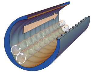
We construct a simplified theory of perturbations, revealing the origin of Langmuir-type vortices. Our geometry is illustrated in figure 1(a), consisting of an infinitely long circular pipe whose walls are augmented by the addition of a pattern of crossing waves. The steepness of these ‘wall waves’ measured in the streamwise direction is presumed to be small:  $\varepsilon =k_1a\ll 1$ where
  $a$ is the waves’ amplitude and
  $k_1$ their streamwise wavenumber. The amplitude is also presumed much smaller than the radius,
  $a/R\ll 1$. We proceed in increasing orders of
  $a$ assuming a basic flow of parabolic Poiseuille form with centreline velocity
  $U_0$.
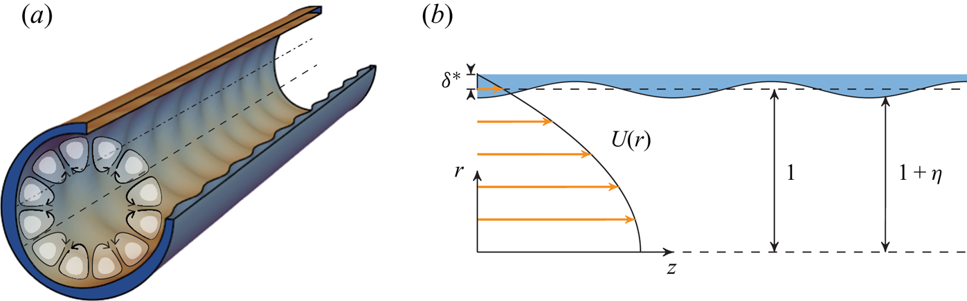
Figure 1. (a) Pipe geometry for  $m_1=3, \kappa=(k_1^2 + m_1^2)^{1/2} =5$; crestlines (dash-dot) and saddle-point lines (dash) are shown; (b) geometry and parameters used in § 2. m 1 and k 1 are, respectively, the azimuthal and streamwise wave numbers of the imprinted ‘wall-wave’ pattern, nondimensionalised with pipe radius.
We first non-dimensionalise using pipe radius  $R$ and
  $U_0$ of the basic flow
 \begin{equation} (r,z,a)\mapsto (r,z,a)R,\quad k\mapsto kR^{{-}1},\quad t \mapsto t R/U_0,\quad \hat{p} \mapsto \hat{p}\rho U_0^{2},\quad \boldsymbol{u}\mapsto\boldsymbol{u} U_0, \end{equation}
where  $\boldsymbol{u}$ here denotes any measure of fluid velocity,
  $\rho$ is the fluid density and
  $\hat{p}$ the pressure perturbation on top of the constant pressure gradient driving the mean flow. (r, θ, z) are the conventional cylindrical co-ordinates. We ignore gravity throughout. The bounding surface is now perturbed slightly and is found at
  $r=1+\hat{\eta} (\theta,z)$ where
  $|\hat{\eta} |\sim a\ll 1$.
We write the resulting three-dimensional velocity field as
 \begin{equation} {\boldsymbol{u}} (r,\theta,z,t)=U(r) \boldsymbol e_z + \hat{\boldsymbol{u}}(r,\theta,z,t), \end{equation}
where  $U(r)$ is the known unperturbed streamwise velocity – the velocity field which we would observe were the pipe a smooth cylinder – and
  $\boldsymbol{\hat{u}} = (\hat{u}_r,\hat{u}_\theta , \hat{u}_z)$ is a small velocity perturbation due to the wall undulations. The Navier–Stokes and continuity equations and their boundary conditions at the wall read
 $$\begin{gather} \left.\begin{aligned} \partial_t\boldsymbol{\hat{u}} + ({\boldsymbol{u}} \boldsymbol{\cdot} \boldsymbol{\nabla}){\boldsymbol{u}} + \boldsymbol{\nabla} \hat{p} = Re^{{-}1} \nabla^{2}\boldsymbol{{u}}\\ \boldsymbol{\nabla}\boldsymbol{\cdot}\boldsymbol{\hat{u}} =0 \end{aligned}\right\};\quad 0 \leq r\leq 1+\hat{\eta}(\theta,z), \end{gather}$$
 $$\begin{gather}\left.\begin{aligned} {\boldsymbol{u}} \boldsymbol{\cdot}\boldsymbol{\nabla} \hat{\eta} = \hat{u}_r \\ [\text{viscous wall condition}] \end{aligned}\right\};\quad r = 1+ \hat{\eta} (\theta,z), \end{gather}$$
where we define the Reynolds number as 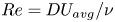 $Re=DU_{avg}/\nu$ where
  $U_{avg}$ is the average velocity,
  $D=2R$ the diameter and
  $\nu$ the kinematic viscosity. The viscous wall boundary condition is treated differently at linear and second order as explained below. In the theory we use the approximate
  $Re = RU_0/\nu$ since the flow is assumed similar to normal Poiseuille flow for which
  $U_{avg}= {\frac 12} U_0$. Solutions must be smooth at
  $r=0$, and the basic flow is assumed to satisfy the equations of motion.
Viscosity is treated in a somewhat indirect manner; it manifests primarily in the ‘zeroth-order’ profile of the unperturbed current,  $U(r)$, which satisfies no-slip boundary conditions at
  $r=1$ and provides the
  ${\textit{O}}(1)$ azimuthal vorticity created by wall friction.
Next, the linear-order solution is found. Rather than attempt to solve an Orr–Sommerfeld-like equation in a cylindrical geometry satisfying the no-slip condition at the wavy wall (which, even if we could, would likely be too involved to be instructive), we make use of a simple model in the vein of Craik (Reference Craik1970) which captures the kinematics of how streamlines near the wall are displaced by the wavy pattern. Noticing that the wave-like first-order perturbation velocities are stable also in the absence of viscosity when  $\hat{\eta}$ is small, and may be assumed virtually unaffected by viscosity (this no longer holds as
  $\hat{\eta}$ increases, as we shall see), they approximately solve a steady inviscid and linearised form of (2.3), except that an appropriate wall boundary condition must be devised.
We assume that the boundary flow creates a displacement thickness  $\sim \delta ^{*}$ near the undulating wall and that the physical pipe wall is at
  $r=1+\delta ^{*} + \hat{\eta} (\theta ,z)$. Next, we impose free-slip boundary conditions at a displaced boundary
  $r=1+\hat{\eta} (\theta ,z)$ – see figure 1(b). Hence, the shape
  $\hat{\eta}$, which we specify does not quite equal the wall shape in the simulations, yet while direct quantitative comparison is not possible, this model makes for a simple theory which is able to elucidate the nature of the Langmuir mechanism.
Lowercase variables, which are small, are assumed to be steady and inviscid, and we expand them in powers of  $a$ (formally identical to an expansion in the steepness parameter
  $\varepsilon$) according to
 \begin{equation} q(r,\theta,z) = {\tfrac 12} q_1(r)\exp(\mathrm{i} m \theta + \mathrm{i} k z) + \mathrm{c.c}. + {\textit{O}}(\varepsilon^{2})\text{ harmonics}, \end{equation}
where  $q$ is any small field quantity and subscript ‘
 $1$’ denotes the linear solution, and ‘c.c.’ means the complex conjugate. m and k are real constants, the azimuthal and streamwise wavenumbers of the ansatz solution (2.4), respectively, where m is an integer.
The governing linearised Euler and continuity equations (2.3a) now read
 $$\begin{gather} \mathrm{i} k U u_{r,1} ={-}p'_1 \end{gather}$$
 $$\begin{gather}\mathrm{i} k U u_{\theta,1} ={-} (\mathrm{i} m/r)p_1 \end{gather}$$
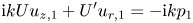 $$\begin{gather}\mathrm{i} k U u_{z,1} + U' u_{r,1} ={-}\mathrm{i} k p_1 \end{gather}$$
 $$\begin{gather}(ru_{r,1}) ' +\mathrm{i} m u_{\theta,1} + \mathrm{i} k ru_{z,1} = 0. \end{gather}$$
Primes ( $'$) denote the derivative with respect to
  $r$. We eliminate velocity components from (2.5) and obtain a Rayleigh-like boundary value problem for the first-order perturbation pressure
  $\hat{p}_1$,
 $$\begin{gather} p_1''+{ \left( \frac 1r - 2\frac{U'}{U} \right) }p_1'-{ \left( \frac{m^{2}}{r^{2}}+k^{2} \right) }p_1 = 0 \end{gather}$$
 $$\begin{gather}p_1(0)=p_1'(0)=0;\quad p_1'(1) = [k U(1)]^{2} \eta. \end{gather}$$
Boundary conditions for  $p_1$ were found from (2.3b) using (2.5a);
  $p_1(r)$ is found numerically from (2.6) using a standard solver for ordinary differential equations.
Armed with the linear-order solution, we proceed to the second order in  $\hat{\eta}$. Although the formalism is different due to the cylindrical rather than planar geometry, the procedure is similar in outline to that of Akselsen & Ellingsen (Reference Akselsen and Ellingsen2020), hence the presentation here is comparatively briefer. Assume boundary undulations composed of two crossing sinusoidal waves directed symmetrically about the streamwise direction
  $z$
$z$
 \begin{equation} \hat{\eta} = \frac{a}{4}[\exp({\mathrm{i}( k_1 z + m_1 \theta)})+ \exp({\mathrm{i}(k_1 z - m_1 \theta)})+ \mathrm{c.c.}]=a\cos(k_1 z)\cos(m_1 \theta).\end{equation}
We impose axial wavenumber  $k_1>0$ and the integer azimuthal wavenumber
  $m_1\geq 1$ (the case
  $m_1=0$ corresponds to alternating axisymmetric contractions and expansions, considered e.g. by Hsu & Kennedy (Reference Hsu and Kennedy1971), Mahmud, Islam & Das (Reference Mahmud, Islam and Das2001), Nishimura et al. (Reference Nishimura, Bian, Matsumoto and Kunitsugu2003) and Jane (Reference Jane2018), and would not trigger the CL1 mechanism). The first-order wave modes involved each have amplitudes
  $a/4$ and the four wave vectors
  $(\pm k_1,\pm m_1)$ (signs varied individually). Second-order harmonics, in turn, are of the same mathematical form with wave vectors which are sums of pairs of these, thus being of four different types with wave vectors
  $\pm 2(k_1,m_1)$,
  $(0,0)$,
  $(\pm 2k_1,0)$ and
  $(0,\pm 2m_1)$. The three first types remain of order
  $a^{2}$ and can be neglected, whereas we retain the last type of harmonic, which turns out to be resonant with a wave vector modulus
  $2m_1$, and grows linearly with time as
  $a^{2} t$ until further development is checked by viscous damping (the resonant, linearly growing solution is given in Appendix A; for an extensive discussion of the planar sibling system, see Akselsen & Ellingsen Reference Akselsen and Ellingsen2020). The resonance will manifest in the formation of
  $\mu =2m_1$ pairs of streamwise vortices, as sketched in figure 1(a). All second-order fields henceforth are understood to be of form
  $\hat{q}_2(r,\theta ,z,t) = \breve {q}(r,t)\exp (\mathrm {i} \mu \theta )+\hbox{c.c.}$ with
  $\breve {q}\in \{\breve {u}_r,\breve {u}_\theta ,\breve {u}_z,\breve {p}\}$; note that these are independent of
  $z$, and hence constitute secondary motion in the
  $(r,\theta )$ plane. The second-order Navier–Stokes and continuity equations then read
 $$\begin{gather} \mathcal{D} \breve{u}_r + \frac{2\mathrm{i} \mu}{r^{2} Re}\breve{u}_\theta + \partial_r \breve{p} ={-} (\boldsymbol{u}_1\boldsymbol{\cdot}\boldsymbol{\nabla}) u_{r,1}, \end{gather}$$
 $$\begin{gather}\mathcal{D} \breve{u}_\theta - \frac{2\mathrm{i} \mu}{r^{2} Re} \breve{u}_r + \frac{\mathrm{i} \mu}{r}\breve{p}={-} (\boldsymbol{u}_1\boldsymbol{\cdot}\boldsymbol{\nabla}) u_{\theta,1}, \end{gather}$$
 $$\begin{gather}\mathcal{D} \breve{u}_z + U'(r)\breve{u}_r - \frac{1}{r^{2} Re}\breve{u}_z ={-}(\boldsymbol{u}_1\boldsymbol{\cdot}\boldsymbol{\nabla}) u_{z,1}, \end{gather}$$
 $$\begin{gather}(r\breve{u}_r)' + \mathrm{i} \mu\breve{u}_\theta = 0. \end{gather}$$
Here,  $\mathcal {D} = \partial _t -Re^{-1} [ \partial _r^{2} + r^{-1} \partial _r - r^{-2}(1+\mu ^{2})]$ and only the resonant interaction is retained in the right-hand side expressions in (2.8).
We find it most convenient now to work with the radial velocity component. Upon eliminating the second-order axial and azimuthal velocities and pressure, one retrieves an inhomogeneous Orr–Sommerfeld-type equation
 $$\begin{gather} \frac{1}{r^{2}}\partial_r\left\{ r \mathcal{D} \left[ \partial_r{ \left( r \breve{u}_r \right) } \right] \right\} - \frac{\mu^{2}}{r^{2}}{ \left( \mathcal{D} - \frac{4}{r^{2} Re} \right) }\breve{u}_r = \mathcal{R}(r); \end{gather}$$
 $$\begin{gather}\mathcal{R}(r) = 8{ \left( \frac{m_1}{rk_1 U } \right) }^{2}\frac{U'}{U} \left[ { \left( k_1^{2}-\frac{m_1^{2}}{r^{2}} \right) }p_1^{2} + (p_1')^{2} \right] \end{gather}$$
for the radial second-order velocity  $\breve {u}_r(r,t)$. Note that
  $\mathcal {R}$ and
  $\breve {u}_r$ are proportional to
  $a^{2}$.
Equation (2.9) permits fairly simple analytical solutions in the two opposite cases of transient inviscid flow ( $Re^{-1}= 0$) and stationary viscous flow (
 $\partial _t\cdot \rightarrow 0$) representing the onset and ultimate stages of vortex development, respectively. We consider here only the latter, which will inform the steady state reached in the simulations. For completeness, the solution for the initial growth rate is presented in Appendix A.
Assuming a steady state with finite  $Re$, (2.9) has solution
 \begin{align} \breve{u}_r(r) &=
\frac{r^{3} Re}{8 \mu}\sum_{s={\pm} 1}
\left\{\sum_{\sigma={\pm} 1} \frac{1}{\sigma+s \mu}
\int_1^{r} \mathrm d \rho{ \left( \frac \rho r \right)
}^{s+ \sigma \mu+3} \mathcal{R} (\rho) \right.\nonumber\\
&\quad \left.\vphantom{\sum_{\sigma={\pm} 1}
\frac{1}{\sigma+s \mu}\int_1^{r}} -\int_1^{0} \mathrm d
\rho\left[ \frac{1}{1+s\mu} + \frac{s r^{2\mu}}{\rho^{1+s}}
{ \left( 1\,{-}\,\rho^{2}\,{-}\,
\frac{1-\rho^{2}+s(1+\rho^{2})}{2(1-s\mu)} \right) }
\right] { \left( \frac{\rho}{r} \right) }^{s+\mu+3}
\mathcal{R} (\rho)\right\} ,
\end{align}
\begin{align} \breve{u}_r(r) &=
\frac{r^{3} Re}{8 \mu}\sum_{s={\pm} 1}
\left\{\sum_{\sigma={\pm} 1} \frac{1}{\sigma+s \mu}
\int_1^{r} \mathrm d \rho{ \left( \frac \rho r \right)
}^{s+ \sigma \mu+3} \mathcal{R} (\rho) \right.\nonumber\\
&\quad \left.\vphantom{\sum_{\sigma={\pm} 1}
\frac{1}{\sigma+s \mu}\int_1^{r}} -\int_1^{0} \mathrm d
\rho\left[ \frac{1}{1+s\mu} + \frac{s r^{2\mu}}{\rho^{1+s}}
{ \left( 1\,{-}\,\rho^{2}\,{-}\,
\frac{1-\rho^{2}+s(1+\rho^{2})}{2(1-s\mu)} \right) }
\right] { \left( \frac{\rho}{r} \right) }^{s+\mu+3}
\mathcal{R} (\rho)\right\} ,
\end{align}
where no-slip boundary conditions at the wall are imposed. The streamwise velocity is
 \begin{equation} \breve{u}_z(r) =\frac{Re}{2\mu} \sum_{s={\pm} 1} s { \left( \int_1^{0} \mathrm d\rho \frac{\rho^{\mu}}{r^{ s\mu}} - \int_1^{r}\mathrm d\rho \frac{\rho^{ s\mu}}{r^{s\mu}} \right) }\rho U'(\rho) \breve{u}_r(\rho).\end{equation}
Thus, the radial and streamwise velocity perturbations scale as  $Re$ and
  $Re^{2}$, respectively. Assuming
  $U'(r)<0$,
  $\breve {u}_r$ and
  $\breve {u}_z$ are of the same sign, so the secondary motion accelerates the mean flow in areas where the circulation jets towards the wall, and vice versa.
The second-order vortical motion being independent of  $z$ we introduce a streamfunction
  $\psi$ whose contours are streamlines. By definition
  $\hat{u}_{r,2} = r^{-1} \partial _\theta \hat{\psi}$ and
  $\hat{u}_{\theta,2} = -\partial _r\hat{\psi}$. In terms of the streamfunction amplitude
  $\breve {\psi }(r) = 2r\breve {u}_r/\mu$ we find
 \begin{equation} \hat{\psi}(\theta,r) = \breve{\psi}(r) \sin(\mu \theta),\quad \hat{u}_z(\theta,r) = 2 \breve{u}_z(r) \cos(\mu \theta), \end{equation}
from which  $\hat{u}_\theta$ can be inferred if required.
3. Theoretical predictions
While the theory in § 2 is simplistic and captures only one of the causes of secondary flow, its predictions are instructive and will inform our DNS study below. We consider only  $m_1\leq 3$ below; higher values create more and smaller vortices closer to the wall but there is no indication of further change of behaviour. Since our second-order solution involves only a single azimuthal wavenumber,
  $m=m_1$, we drop the subscript ‘1’ from wall-wavevector components henceforth.
Assume a laminar bulk flow profile of Poiseuille type,
 \begin{equation} U(r) = 1 - r^{2}/(1+\delta^{*})^{2} \end{equation}
stretched a displacement length  $\delta ^{*}$ beyond the pipe radius, as sketched in figure 1(b). Henceforth, we use the term crestline to denote a curve following the wall at constant polar angle
  $\theta = n{\rm \pi} / m,\ n=0,\ldots ,2\;m -1$, running over the maxima of crests and troughs, and saddle-point line for the nearly straight line following the wall midway between these. Streamlines close to crestlines have the largest undulations in wall-attached flow.
A key parameter is the angle  $\varphi = \arctan (m/k)$ between the streamwise and azimuthal wavenumbers of the wall undulation, which we refer to as the crossing angle. We let
  $0\leq \varphi \leq 90^{\circ }$. We shall refer to geometries
  $\varphi < 45^{\circ }$,
  $=45^{\circ }$ and
  $>45^{\circ }$ as contracted, regular and protracted egg-carton patterns, respectively. The theoretical dependence of the circulation strength on
  $\varphi$ is investigated in figure 2, where the wave vector modulus
  $\kappa =(m^{2}+k^{2})^{1/2}$ is kept constant at three different values while
  $\varphi$ changes. Figure 2(a) shows the steady-state circulation strength, represented by the extremum of
  $\psi /Re\, a^{2}$ along a ray at
  $\theta ={\rm \pi} /4m$ running approximately through the centre of the ‘first’ vortex. The integer
  $m_1$ can only take values
  $1,2,\ldots ,{floor}(\kappa )$, shown with vertical lines labelled with corresponding azimuthal wavenumber
  $m$. Corresponding pipe patterns are shown in figure 2(e). The volume flow rate through a vortex cross-section is proportional to
  ${max}|\psi |$, and the sign of
  $\psi$ shows the rotational direction: relative to the pipe wall
  $\psi >0$ indicates flow towards crestlines and away from saddle-point lines, and vice versa.

Figure 2. Theoretical predictions. (a) Circulation intensity for fixed  $\kappa$ as a function of phase angle
  $\varphi$;
  $\delta ^{*}=0.05$. Only design configurations for which
  $m$ is an integer are realisable; these are marked with dashed vertical lines where
  $m_1$ values are marked as integers. (b–d) Streamlines in the cross-flow plane for
  $m\in \{1,2,3\}$ and
  $\kappa ={\rm \pi}$, which are contours of
  $\hat{\psi}$. Velocity field vectors are shown for
  $m=1$ whereas arrows in (c,d) merely indicate flow direction. Circulation intensity may be inferred from (a) considering
  $\kappa ={\rm \pi}$. Pipe cross-section outlines are shown at the crests/troughs of the wavy pattern (
 $z=\lambda /4$ and
  $3\lambda /4$ with
  $\lambda =2{\rm \pi} /k$). Colours illustrate the value of
  $\psi$ with light (dark) being positive (negative). (e) Pipe design configurations corresponding to the dashed vertical lines in (a);
  $45^{\circ }$ is marked with a solid vertical line.
Several observations are made. The circulation intensity is relatively insensitive to wavenumber amplitude  $\kappa$ but highly sensitive to
  $\varphi$. The Langmuir driving mechanism is very weak near
  $\varphi = 45^{\circ }$, the only angle previously investigated for pipe flow to our knowledge, and
  $\hat{\psi}$ changes sign near this angle. (We note in passing that the secondary flow observed in turbulent pipe flow at
  $\varphi =45^{\circ }$ by Chan et al. (Reference Chan, MacDonald, Chung, Hutchins and Ooi2018), corresponded to negative
  $\psi$.) Moreover, the intensity of the ‘reversed’ Langmuir rotation at
  $\varphi >45^{\circ }$ is considerably weaker than that predicted for smaller angles
  $\varphi \lesssim 30^{\circ }$. We note with interest, and for future reference, that the swirl changes sign close to the pipe wall for
  $\varphi =45^{\circ }, 60^{\circ }$ and
  $Re_\tau =40,60$.
Figure 2(b–d) shows streamlines  $\psi =\text {const}$ of the flow averaged over an axial wall wavelength, for the three possible angles when
  $\kappa ={\rm \pi}$. Notice again the reversal of rotation direction for
  $m=3$ where the pattern is protracted.
4. Simulations
We proceed now to study the real flow in the wavy pipe geometry using DNS, focussing on the effects of the wave crossing angle  $\varphi$, Reynolds number and topography amplitude. Further plots and figures for all simulation cases may be found in the Supplementary Materials. Velocities are in units of the mean centreline velocity for each case.
The numerical simulations were conducted using NEK5000, a high-fidelity spectral element code (Fischer, Lottes & Kerkemeier Reference Fischer, Lottes and Kerkemeier2008). Each computational domain contains  $1280$ macro-elements with
  $10$ macro-elements in the streamwise direction. The nodes inside of the element are distributed using the Gauss–Lobatto–Legendre points and a polynomial order of
  $7$ is used, resulting in approximately
  $655\,360$ grid points in total. The grid points on the no-slip, impermeable wall of the pipe conform to the roughness topography, the domain length equals to one roughness period and the ends of the pipe are periodic. The third-order time-stepping scheme and the
  $P_N-P_{N-2}$ method introduced by Maday & Patera (Reference Maday and Patera1989) was used for the simulations. A constant pressure gradient is used to drive the flow and the simulations were run with a constant time-step ranging from
 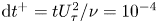 $\mathrm {d} t^{+} = t U_\tau ^{2}/\nu = 10^{-4}$ to
  $2\times 10^{-4}$ (
 $U_\tau = \sqrt {\tau _w/\rho }$ is the friction velocity,
  $\tau _w$ the mean wall shear stress) to ensure that the Courant number is less than 1. The simulations were initialised with a laminar smooth-wall flow and were run for a duration of at least
  $t^{+} = 1600$, where the flow has converged to a steady state. A domain length study was conducted for
  $\varphi = 18.6$ with a = 0.05 at
  $Re_\tau = 80$ and no changes to the steady-state flow were observed when the length of the pipe was increased by
  $6$ and
  $10$ times. In simulations the phase of the surface deformation is such that
  $\eta (\theta ,z) = a\sin (kz)\sin (m\theta )$.
One primary observation we make through a broad parameter study in this section is that a competition occurs between two effects, both of which drive secondary motion, in opposite senses. One is a dynamic effect due to increased wall shear stress where the roughness is increased near crestlines, the other is the kinematic Langmuir circulation effect, CL1. The former causes secondary flow in the negative sense as defined, the latter drives positive-sense rotations for  $\varphi \lesssim 30^{\circ }$ where it is strongest in accordance with theory.
It is highly useful for our further analysis to introduce streamwise-averaged quantities. Noting that our flow is steady and periodic with streamwise period (or wavelength)  $\lambda = 2{\rm \pi} / k$ we define the averaging operator
 \begin{equation} \overline{(\cdots)} = \frac 1{\lambda}\int_0^{\lambda}(\cdots)\,\mathrm{d} z. \end{equation}
 Based on the principle of volume flux, a measure of circulation strength in the simulated flows is found as the approximate streamfunction amplitude  $\acute{\psi}$ along a radial line of constant polar angle
  $\theta =\theta _0$ running through, or nearly through, the centre of a vortex. We choose
  $\theta _0={\rm \pi} /4 m$ as in the previous section, and define
 \begin{equation} \acute{\psi}(r;\theta_0) = \int_{0}^{r} \mathrm d \rho \overline{\hat{u}_\theta}(\theta_0,\rho). \end{equation}
4.1. Parameter studies
The dependence of the circulation strength on crossing angle  $\varphi$ and
  $Re$ is studied in figure 3; rows 1–3 have constant
  $Re_\tau$, columns 1–3 have constant
  $\varphi$. All graphs are of
  $\acute {\psi }/Re\, a^{2}$. Note that in all plots of quantities averaged over a streamwise wave period, linear effects of wall undulations vanish and only contributions from (even) higher orders remain.
Figure 3. Simulation results,  $a=0.05,\kappa ={\rm \pi}$ and
  $m=1$. Here,
  $Re_\tau$ is the same in the first three rows, and
  $\varphi$ is the same in the first three columns, as indicated. (a–c, e–g, i–k) Black curves are contours of
  $\acute {\psi }/(Re\, a^{2})$ indicating streamlines, arrows indicate flow direction; colour contours show deviation of the total streamwise velocity
  $\overline {u_{z,{tot}}}$ from Poiseuille flow as defined in (4.5). (d,h,l,m–o) Plots of
  $\acute {\psi }/(Re\, a^{2})$ along the ray
  $\theta ={\rm \pi} /4$. A common legend applies to all plots where
  $\varphi$ varies at constant
  $Re_\tau$ (d,h,l), and vice versa (m–o).
We investigate three different crossing angles,  $\varphi =18.6^{\circ }, 45^{\circ }$ and
  $60^{\circ }$. According to theory, Langmuir motion should be strongest and positive for the first angle, and much weaker for the two latter; see figure 2(b). Indeed, the most striking feature in figure 3 is arguably that the smallest angle shows positive circulation (a,e,i), the other two negative (b,c,f,g,j,k). However, unlike in the theoretical graph of the Langmuir effect alone, figure 2, the oppositely directed circulation at
  $45^{\circ }$ and
  $60^{\circ }$ is not weak, but of comparable magnitude as for
  $18.6^{\circ }$, evidence of another mechanism at play. We propose that there is a dynamic, viscosity-driven forcing of negative circulation present due to the azimuthally varying roughness producing alternating regions of higher and lower momentum, as observed by Chan et al. (Reference Chan, MacDonald, Chung, Hutchins and Ooi2018), which depends only weakly on
  $\varphi$. The competing Langmuir effect is significant only for the smallest angle. Indeed, in all simulations, the flows at
  $45^{\circ }$ and
  $60^{\circ }$ are highly similar, whereas the
  $18.6^{\circ }$ flow is strikingly different (see also supplementary material available at https://doi.org/10.1017/jfm.2021.696).
4.1.1. Sensitivity to Reynolds numbers and crossing angle  $\varphi$

We define  $Re_\tau =U_\tau R/\nu$ and
  $Re=U_{avg}D/\nu$, where
  $U_{avg}$ is the total flow rate divided by
  ${\rm \pi} R^{2}$. For Poiseuille flow,
  $Re= {\frac 12} Re_\tau ^{2}$.
Figure 3 shows simulation results for  $a=0.05$ and
  $m=1$, varying
  $\varphi$ along rows and
  $Re_\tau$, along columns. Three different topography angles
  $\varphi = 18.6^{\circ }$,
  $45.0^{\circ }$ and
  $60.0^{\circ }$ – contracted, regular and protracted egg carton, respectively – are shown, and three different
  $Re_\tau =40,60,80$. All panels show values of
  $\acute{\psi} (r,{\rm \pi} /4m)/(Re\, a^{2})$ either as contours or graphs. The highest Reynolds number based on average velocity achieved in the reported simulations is
  $2751$. A simulation at
  $Re_\tau =100$ became turbulent (not included since the grid used herein is too coarse to properly capture turbulent flow). Our simulations are not sufficient to draw confident conclusions about stability in each case, which remains a question for the future.
Studying the bottom row of figure 3, we observe that the expected scaling  $\acute{\psi} \propto Re$ is reasonably well satisfied throughout the laminar regime for regular and protracted egg carton, whereas for the contracted egg carton the scaling is far more imperfect. In fact, for
  $\varphi = 18.6^{\circ }$,
  $\acute{\psi}$ increases faster than linearly with
  $Re$, a curious observation we discuss further in § 4.1.3. The departure from the scaling predicted by inviscid theory can be traced back to a greater deviation between the theoretical, inviscid first-order velocity field and that from simulations, an indication that viscous effects in the boundary layer influence the results considerably in a non-trivial way, more strongly for the contracted pattern. A partial explanation is that, for one and the same
  $\kappa$, smaller
  $\varphi$ corresponds to higher steepness
 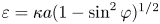 $\varepsilon =\kappa a (1-\sin ^{2}\varphi )^{1/2}$, and higher-order nonlinear effects manifest more easily. We subject this curious observation to closer scrutiny in § 4.1.3.
It is instructive to regard the pressure field across the pipe section when averaged along a streamwise wavelength so that linear-order perturbations vanish, leaving a mean pressure deviation able to drive steady secondary motion. Compare the pressure fields in figure 4(e,f,l) wherein  $\varphi =45^{\circ }, 60^{\circ }$ and
  $18.6^{\circ }$, respectively, for
  $a=0.05$. The flow and pressure perturbations for the two former are similar: high pressure regions above crestlines push the flow away from the wall there, driving vortices in the negative sense. This might intuitively be expected since the flow suffers higher friction here than along the straighter saddle-point lines. The pressure field for
  $18.6^{\circ }$ on the other hand shows the opposite: low-pressure regions above crestlines attract the secondary flow setting up positive-sense vortices.
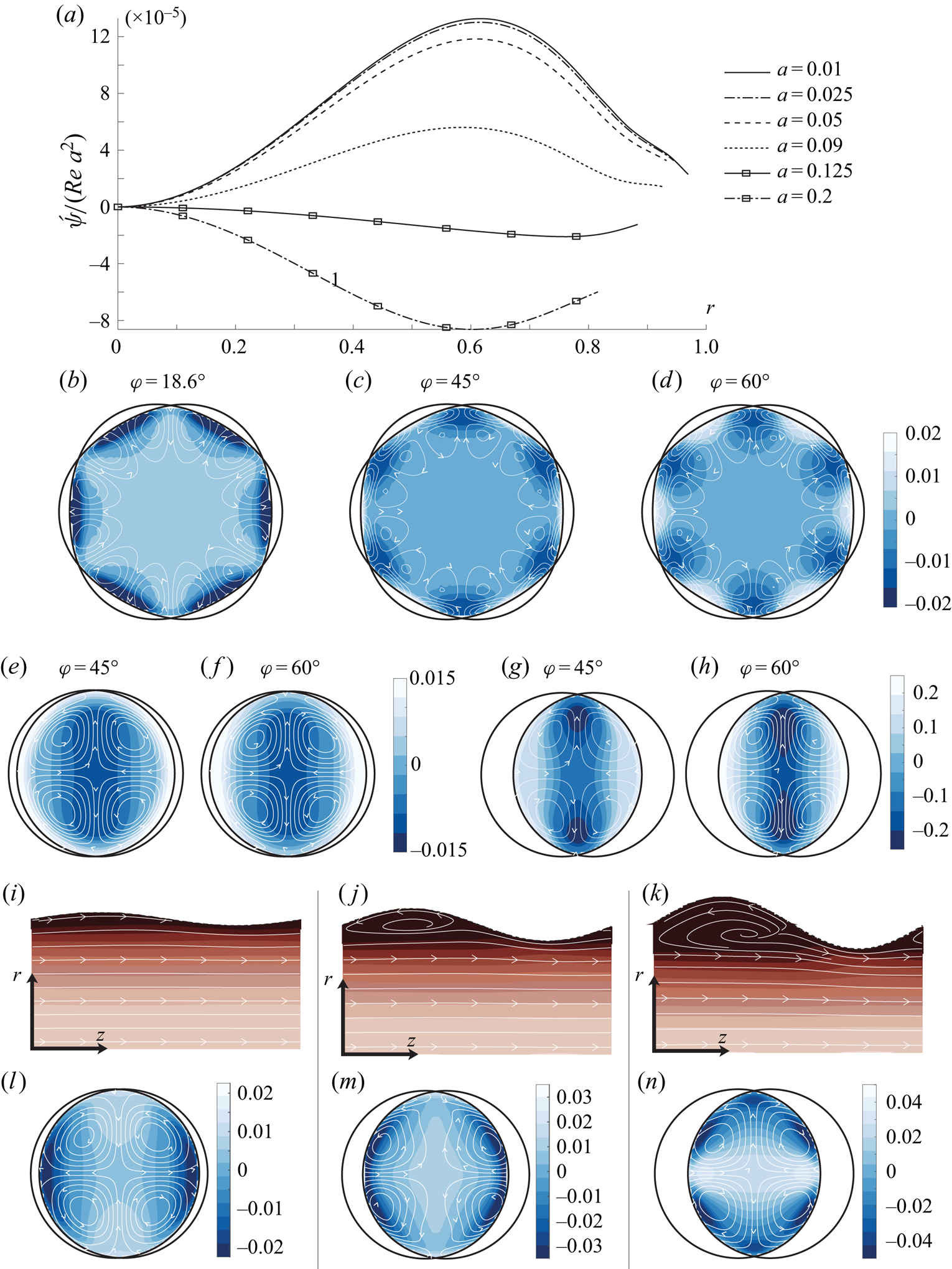
Figure 4. Simulation results with  $Re_\tau = 40$. (a) Scaled circulation strength along
  $\theta ={\rm \pi} /4m$ for
  $\varphi = 18.6^{\circ }, m_1=1$ and increasing
  $a$; graphs from top to bottom:
  $a=0.01, 0.025, 0.05, 0.09,0.125,0.2$. (b–h, l–n) Streamwise-averaged flow (streamlines) and pressure (colour contours, average pressure subtracted). Panels (b–d) have
  $m = 3$, all other panels
  $m = 1$. Crossing angle
  $\varphi =18.6^{\circ }$ except as indicated. Amplitudes are
  $a=0.05$ (b–f,i,l),
  $a=0.125$ (j,m),
  $a=0.2$ (g,h,k,n). (i–k) Streamlines in a streamwise section of the pipe through crests/troughs at
  $\theta ={\rm \pi} /2$, lighter (darker) colour indicates higher (lower) average absolute velocity.
Our suggested interpretation is, as we began to argue above: the dynamic friction mechanism evident in figure 4(e,f) will be present for all three values of  $\varphi$ in roughly equal measure; the strong similarity between figures 4(b) and 4(c) indicates that it varies little with
  $\varphi$ so long as the flow does not separate. On the other hand, the Langmuir mechanism is far stronger for
  $\varphi =18.6^{\circ }$ than for the two higher values (see figure 2a), and therefore ‘wins’ the competition there.
4.1.2. Sensitivity to amplitude
Interestingly, when increasing the amplitude  $a$, circulation reversal is observed for
  $\varphi =18.6^{\circ }$. We again propose an explanation in terms of the two competing mechanisms for secondary flow. In figure 4(a) we plot the scaled circulation strength
  $\tilde \psi /\textrm {Re} \,a^{2}$ in the protracted egg-carton geometry for increasing amplitudes up to
  $a=0.2$. The predicted
  ${\sim }a^{2}$ scaling is accurate for moderate amplitudes
  $a \leq 0.05$, but beyond this point a dramatic reduction occurs, and as
  $a\gtrsim 0.1$ the direction of rotation reverses with
  $|\acute{\psi} |/a^{2}$ eventually reaching comparable values.
We find the reason to be the onset of flow separation affecting the two mechanisms differently. The Langmuir swirling is driven by the kinematic sinusoidal deflection of streamlines; once the flow separates in the troughs, streamlines no longer follow the wall's shape (see figure 4i–k) and a further increase in  $a$ does not further increase the ‘effective amplitude’ of the streamline undulations. For
  $\varphi =45^{\circ }$ and
  $60^{\circ }$ the wall undulations are less steep in the streamwise direction and the flow does not separate, approximately retaining the
  ${\sim }a^{2}$ scaling.
4.1.3. Circulaton strength vs increased drag
It is of interest to compare the strength of circulation with the increased pressure loss from making the wall surface wavy. Using the definition of the Darcy friction factor  $f=(2gD/U_{avg}^{2})h_L$,
  $h_L$ being the head loss per streamwise wavelength related to
  $\tau _w$ by
  $h_L=2\tau_{w} /\rho g R$ (dimensional units,
  $g$ is gravitational acceleration), gives
 \begin{equation} f = \frac{32 Re_\tau^{2}}{Re^{2}}, \end{equation}
having used  $Re_\tau =(R/\nu )\sqrt {\tau /\rho }$ and
 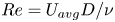 $Re=U_{avg} D/\nu$. We will compare with Poiseuille flow with the same Reynolds number,
 \begin{equation} U_{P}(r) = 2U_{avg}(1-r^{2}), \end{equation}
for which it is readily shown that  $Re^{2}_{P}={\frac 12} Re_\tau ^{2}$ and
  $f_{P}=64/Re$. The relative increase in friction coefficient is thus
 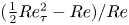 $({\frac 12} Re_\tau ^{2}-Re)/Re$ which we plot in per cent as the abscissa in figure 5.

Figure 5. Maximum circulation strength plotted against increase in friction factor (i.e. increased head loss) in per cent. (a) Comparison of three different crossing angles for  $m=1, a=0.05$ – corresponding values of
  $Re_\tau$ are indicated for each marker (common for overlapping markers); (b) same cases as in (a), but with Reynolds number as abscissa; (c) increasing amplitude for
  $Re_\tau =40$ and
  $m=1$.
A particularly striking observation can be made from figure 5(a), where three different crossing angles  $\varphi$ are compared for
  $a=0.05$ and
  $m=1$. For each angle, each marker corresponds to a different
  $Re_\tau =40,60,80$ increasing from left to right; for
  $\varphi =18.6^{\circ }$ also
  $Re_\tau =20$ is included. The points are too few to fully determine scaling, yet it appears that, whereas for the two larger angles where CL1 is weak the scaled circulation strength
  $\max (|\acute {\psi }|)/Re$ saturates to a constant value, indicating that absolute circulation strength increases as
  ${\sim }\textrm {Re}$ throughout the laminar regime, for the smallest angle with strong Langmuir forcing, circulation strength increases faster than
  ${\sim }Re$. This becomes even clearer when plotted against
  $Re$ as in figure 5(b) (The faster-than-linear scaling was already observed in figure 3m.) The non-monotonic dependence of circulation strength on amplitude previously discussed in § 4.1.2 is illustrated once more in the scatterplot of figure 5(c).
4.1.4. High- and low-momentum paths
High-momentum paths (HMPs) and low-momentum paths (LMPs) are conspicuous in figure 3, where colour contours of
 \begin{equation} \overline{u_z}(r,\theta)=\overline{u_{z,{tot}}}(r,\theta)-U_{P}(r) \end{equation}
are shown. Here,  $U_{P}(r) = 2U_{avg}(1-r^{2})$ is a Poiseuille flow of the same volume flux as the simulated flow. Both for
  $\varphi =45^{\circ }$ and
  $60^{\circ }$ the intuitively expected behaviour is seen: lower (higher) momentum resides over crestlines (saddle-point lines) where the roughness is highest (lowest). At
  $18.6^{\circ }$ the picture is the opposite, yet a telling observation is made in figure 3(a): in a thin layer over the crestline wall a strong velocity deficit from increased friction is in fact present, but is soon overtaken by CL1 away from the wall (in (e,i) the layer is so thin as to fall outside the plotted area). This is another indication that the two effects are simultaneously present and competing. In all cases we note that the rotating motion is directed away from the wall where there is a LMP, and vice versa.
In studies of turbulence over spanwise varying roughness of different kinds, secondary motion has also consistently been directed away from the wall over LMPs and vice versa irrespective of the kind of roughness (e.g. Willingham et al. Reference Willingham, Anderson, Christensen and Barros2014; Anderson et al. Reference Anderson, Barros, Christensen and Awasthi2015; Vanderwel & Ganapathisubramani Reference Vanderwel and Ganapathisubramani2015; Chan et al. Reference Chan, MacDonald, Chung, Hutchins and Ooi2018; Chung, Monty & Hutchins Reference Chung, Monty and Hutchins2018; Hwang & Lee Reference Hwang and Lee2018). Colombini & Parker (Reference Colombini and Parker1995) show that the situation is more subtle when a free surface is present, and Stroh et al. (Reference Stroh, Schäfer, Frohnapfel and Forooghi2020) found a richer pattern of secondary motion when spanwise roughness variations do not create a clear distinction between the two. While we should be careful not to infer too much from turbulent mean flow to the present laminar case, it is consistent with our observations. (We bear in mind the related, but not identical, rule of thumb due to Hinze (Reference Hinze1967) that secondary flow is directed out of (into) areas with net production (dissipation) of turbulent kinetic energy, by which Hwang & Lee (Reference Hwang and Lee2018) explain the apparent inconsistency in the sense of rotation of secondary flows between different types of roughness, compared with, e.g. Wang & Cheng Reference Wang and Cheng2006.)
The direction of swirling for our laminar case is indicated by the streamwise-averaged equation of motion. Into the  $z$-component of the Navier–Stokes equation (2.3a) we insert
  $\overline {u_{z,{tot}}} = U_{P}(r)+\overline {u_z}$. We use rectangular coordinates, but notice that
  $(\overline {u} \partial _x+\overline {v} \partial _y)U_{P} = \overline {u_r} U_{P}'(r) = -4U_{avg} r \overline {u_r}$. Ordering in powers of
  $a$, applying streamwise averaging (4.1) and neglecting terms of
  ${O}(a^{2})$ yields
 \begin{equation} - 2Re\,r\overline{u_r} = \nabla^{2}\overline{u_z} \end{equation}
Near a HMP where  $\overline {u_z}$ has a maximum,
  $\nabla ^{2}\overline {u_z}<0$ and hence
  $\overline {u_r}>0$, and for a LMP the opposite is true, thus flow is towards the wall near a HMP and vice versa. We note from the presence of
  $Re$ that this
  ${O}(a)$ mechanism depends on the presence of viscosity.
We can already see that the direction of secondary flow, upwards from crestlines and down towards saddle-point lines, when Langmuir driving is weak (e.g. for  $\varphi =45^{\circ }$ and
  $60^{\circ }$) is not surprising: fluid paths going over crests and troughs suffer higher friction than the nearly straight saddle-point streamlines, giving rise to a low-momentum channel pushing the flow towards the centre.
5. Analogy of secondary flow in turbulence
Prandtl (Reference Prandtl1952) famously divided secondary flow in turbulence into two categories, now referred to as Prandtl's secondary flow of the first and second kinds, respectively. The former stems from inviscid skewing of the mean flow, typically from the flow being guided by a curved surface; the second kind is driven by the inhomogeneity of Reynolds stresses.
It is commonly stated that Prandtl's secondary flow of the second part has no counterpart in laminar flow (e.g. Bradshaw (Reference Bradshaw1987), p. 54). We argue that this might be open to discussion since we shall see that in streamwise-periodic flow a close analogy is achieved when Reynolds averaging replaced by streamwise averaging, (4.1).
The velocity and vorticity fields may be divided into a mean and an oscillating part
 \begin{equation} \boldsymbol{u} = \overline{\boldsymbol{u}} + \tilde{\boldsymbol{u}};\quad {\boldsymbol \omega} =\overline{{\boldsymbol \omega}} + \tilde{{\boldsymbol \omega}}, \end{equation}
with  $\boldsymbol{u} = (u_r, u_\theta , u_z)$ or
  $(u,v,w)$, and
  ${\boldsymbol \omega } = \boldsymbol {\nabla }\times \boldsymbol{u}= (\omega _r, \omega _\theta , \omega _z)$ or
  $(\omega _x,\omega _y,\omega _z)$, with accents as appropriate.
Let  $\vartheta$ denote any field quantity henceforth. Note the relations
 $$\begin{gather} \overline{\widetilde{\vartheta}} = 0; \end{gather}$$
 $$\begin{gather}\overline{\partial_z \vartheta} = 0; \end{gather}$$
 $$\begin{gather}\overline{\partial_i \vartheta}=\partial_i\overline{\vartheta}, \end{gather}$$
where  $i\in \{ x,y\}$ or
  $\{r,\theta \}$.
For simplicity, we work first in rectangular coordinates; the direction of mean flow remains  $z$. Consider the streamwise component of the vorticity equation. Exactly following the procedure of, e.g. Anderson et al. (Reference Anderson, Barros, Christensen and Awasthi2015) but for the definition of the averaging operator, one finds (with
  $\nabla _\perp ^{2} = \partial _x^{2} + \partial _y^{2}$)
 \begin{equation} (\overline{u}\partial_x + \overline{v} \partial_y)\overline{\omega_z} = \overline{\omega_x}\partial_x \overline{w}+ \overline{\omega_y}\partial_y \overline{w}+ (\partial_y^{2} - \partial_x^{2})R_{xy}+ \partial_x\partial_y(R_{xx} - R_{yy})+\nu\nabla_\perp^{2}\overline{\omega_z}, \end{equation}
where we define the undulation stress
 \begin{equation} R_{xx} = \overline{\tilde{u}\tilde{u}};\quad R_{yy} = \overline{\tilde{v}\tilde{v}};\quad R_{xy} = \overline{\tilde{u}\tilde{v}}. \end{equation}
Replacing streamwise averaging with Reynolds averaging, (5.3) is a classic one (Bradshaw Reference Bradshaw1987). The undulation stresses are analogous to what in turbulence is often dubbed dispersive stress (Raupach & Shaw Reference Raupach and Shaw1982) arising from spatial correlation of time-averaged quantities; we eschew this term to avoid any confusion with dispersion of surface waves, featuring in the literature on Langmuir circulations.
In a turbulent flow, the first two terms on the right-hand side of (5.3) would correspond to Prandtl's first kind of secondary flow. These add to zero in streamwise-periodic flow, which is obvious once we note that  $\overline {\omega _x} = \partial _y \overline {w}$ and
  $\overline {\omega _y} = -\partial _x \overline {w}$.
We are left with the terms involving the undulation stresses, which may be written in the following two forms
 \begin{align} (\overline{u}\partial_x + \overline{v} \partial_y)\overline{\omega_z} &= S_{norm} +S_{shear}+\nu\nabla_\perp^{2}\overline{\omega_z} \end{align}
 \begin{align} &= S_{def} + S_{adv}+\nu\nabla_\perp^{2}\overline{\omega_z}, \end{align}
with
 \begin{align} S_{norm} &= \partial_x\partial_y(R_{xx} - R_{yy});\quad S_{shear} = (\partial_y^{2} - \partial_x^{2})R_{xy};\\ S_{def} &= \overline{(\tilde{{\boldsymbol \omega}}\boldsymbol{\cdot}\boldsymbol{\nabla})\tilde{w}} = {\tfrac 12} S_{norm} + S_{shear} + \partial_x\overline{\tilde{u}\partial_x\tilde{v}}-\partial_y\overline{\tilde{v}\partial_y\tilde{u}} \nonumber\\ &= {\tfrac 12} S_\text{norm} +\partial_y\overline{\tilde{u}\partial_y \tilde{v}}-\partial_x\overline{\tilde{v}\partial_x \tilde{u}}; \end{align}
 \begin{align} S_{adv} &={-} \overline{(\tilde{\boldsymbol{u}}\boldsymbol{\cdot}\boldsymbol{\nabla})\tilde{\omega}_z}= {\tfrac 12} S_{norm} - \partial_x\overline{\tilde{u}\partial_x\tilde{v}}+\partial_y\overline{\tilde{v}\partial_y\tilde{u}}. \end{align}
We let the total mean-vorticity production be
 \begin{equation} S_{prod} = S_{norm} + S_{shear} = S_{def} + S_{adv}. \end{equation}
 The form (5.5a) is standard in the turbulence literature, and has the advantage of highlighting the asymmetry of  $R_{ij}$ under
  $x\leftrightarrow y$ as the explicit cause of streamwise vortices, due to normal and shear stresses, respectively. While a natural choice in wall- and channel-type geometries, in our present case we find a physical interpretation of the individual terms less obvious. Going to cylindrical coordinates mixes the roles of normal and shear stresses: by expressing
  $u,v$ in terms of
  $u_r, v_r$ and
  $\theta$ one finds,
 \begin{equation} R_{xx}-R_{yy} = 2 R_{r\theta}\sin 2\theta;\quad R_{xy} ={-}2R_{r\theta}\cos 2\theta+{\tfrac 12}(R_{rr}-R_{\theta\theta})\sin 2\theta, \end{equation}
with  $R_{rr}=\overline {\tilde {u}_r^{2}}, R_{\theta \theta }=\overline {\tilde {u}_\theta ^{2}}$ and
  $R_{r\theta }=\overline {\tilde {u}_r\tilde {u}_\theta }$. Some light might be shed from recasting the full analysis in cylindrical coordinates, but we choose instead to analyse vorticity transport in terms of (5.5b), the form favoured by Nikitin, Pimanov & Popelenskaya (Reference Nikitin, Pimanov and Popelenskaya2019).
The form (5.5b) is advantageous in that the two production terms  $S_{def}$ and
  $S_{shear}$ are independent of the choice of coordinate system. Physically, they correspond, respectively, to production of streamwise-averaged vorticity by periodic deformation and advection of vorticity, respectively.
To proceed, we expand all terms in (5.5) in a Fourier–Bessel series
 \begin{equation} F(r,\theta)= f_0(r) + f_2(r)\sin( 2 m\theta)+ f_4(r)\sin(4 m\theta)+\cdots, \end{equation}
(cosine terms are zero, and odd terms are prohibited by symmetry) where  $F$ is any term and
  $f_0,f_2,f_4\cdots$ are functions. The
  $\sin (\pm 4 m\theta )$ terms largely determine the swirling motion for reasons we now explain.
The mean transport of streamwise-averaged vorticity,  $(\overline {\boldsymbol{u}}\boldsymbol {\cdot }\boldsymbol {\nabla })\overline {\omega _z}$, is shown in figure 6 for the three different crossing angles, with
 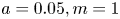 $a=0.05, m=1$ and
  $Re_\tau =40$. We see that, in all cases, the amplitude is similar, of the order of
  $10^{-5}$ in these cases, and the leading contribution is
  ${\propto }\sin (4\;m \theta )$. We observe that the significant transport of mean streamwise vorticity is organised in a pattern of concentric rings. Consider the two innermost rings in all figures (a thin ring very near the edge is also manifest which does not appear to affect the streamwise-averaged flow perceptibly so we shall ignore this fact). In figure 6 we have indicated the inner and outer rings with a circle and square, respectively. For the two larger angles the two rings have similar amplitudes and comparison with the streamlines in figure 3(a–c) shows that the extrema of
  $(\overline {\boldsymbol{u}}\boldsymbol {\cdot }\boldsymbol {\nabla })\overline {\omega _z}$ correspond to oppositely directed rotating motions due to the inner ring in the form of elongated streamline loops confined to an area close to the wall. The larger mean-flow paths correspond to maxima in the inner ring. In comparison, the outer ring in the
  $\varphi =18.6^{\circ }$ case is similar to the other two cases but for being slightly shifted away from the axis, but strikingly, the inner ring is much weaker than the outer, allowing the vortices created by vorticity production in the outer ring to reach into the bulk flow, causing mean rotation in the opposite sense. Apparently, the presence of Langmuir forcing, instead of adding another source of vorticity production, effects a partial cancellation of net inner-ring mean-vorticity production, a conclusion which is surprising to us and should be further investigated in the future.

Figure 6. Mean transport of streamwise-averaged vorticity,  $(\overline {\boldsymbol{u}}\boldsymbol {\cdot }\boldsymbol {\nabla })\overline {\omega _z}$, for
  $a=0.05, m=1$ and
  $Re_\tau =40$. Dashed curves indicate the inner and outer circles of vorticity production, marked with a circle and square, respectively.
To continue we analyse the production contributions due to undulatory motion and the viscous diffusion of average streamwise vorticity. In figure 7 we have calculated and visualised the terms on the right-hand side of (5.5b) in full. Comparing with figure 6, we observe that the magnitude of the right-hand side terms individually are more than two orders of magnitude larger than those on the left-hand side; the vast majority of mean vorticity production  $S_{prod}$ is cancelled by viscous diffusion
  $\nu \nabla _\perp ^{2}\overline {\omega _z}$. The dominant contribution in all panels of figure 7 is
  ${\propto }\sin (2m \theta )$, with higher harmonics only small corrections, and this term cancels in sum, we conjecture, exactly (numerically, its amplitude is consistently beneath the level of numerical noise).


Now, it can be observed from the streamwise-averaged flow patterns that the left-hand side of (5.5) varies no more slowly than 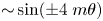 ${\sim }\sin (\pm 4\;m \theta )$ as a function of
  $\theta$. This is in fact a necessity given the observed mean-flow patterns in figures 3 and 4 (and all other simulation cases; see Supplementary Materials) as we now argue. For concreteness, take the
  $m=1$ cases in figure 3 for example. Note that the streamlines are all closed within single quadrants of the cross-section, and consider that the cumulative (integrated) production and diffusion of mean vorticity around a closed streamline must be zero. Since only the
  $f_4$-term and higher take both signs inside a single quadrant, periodicity demands
  $f_0=f_2=0$ for the left-hand side of (5.5), and hence also for the full right-hand side, as a whole. The argument trivially extends to
  $m > 1$, where the same is also invariably observed. We conjecture that the exact cancellation of
  $\sin (2m\theta )$ terms can be proved in general, but consistent observation in both theory and simulation is sufficient for our purposes.
Since the dominant  $\sin (2m\theta )$-mode does not contribute to the net production of mean vorticity, considerably improved clarity is achieved by subtracting it in our plots. Noting that higher harmonics beyond
  $f_4$ make up only a small correction, we retain only the
  $f_4$ term, which is the main driver of vortical motion. Using
 \begin{equation} f_4(r) = \frac 2{\rm \pi} \int_0^{\rm \pi}\mathrm{d}\theta' F(r,\theta')\sin (4m\theta'), \end{equation}
we plot the same production and diffusion terms again in figure 8. We still observe that the majority of production is cancelled by viscous diffusion – the amplitudes in figure 8 are an order of magnitudes higher than those of figure 6. As previously, we again observe that, for the same  $a, m$ and
  $Re_\tau$, the results for
  $45^{\circ }$ and
  $60^{\circ }$ are highly similar (but for an overall factor in figure 8) while the
  $18.6^{\circ }$ is qualitatively different.

Figure 8. Same as in figure 7, but the terms  ${\propto }\sin (4 m\theta )$ only.
Figure 8 tells an interesting story. Consider first  $45^{\circ }$ and
  $60^{\circ }$. Strong production in the outer ring is due to average advection of undulating vorticity, most of which is cancelled by the viscous term. A smaller production in the inner ring due to vorticity deformation is evident in figure 6 for these two angles, and these are not cancelled by viscous diffusion. The indication is that, although weak compared with advection production, due to cancellations this inner-ring production nevertheless drives the prevailing secondary motion evident in streamline plots e.g. in figure 3 (note the difference in scale between figures 6 and 8).
The picture for  $18.6^{\circ }$ is strikingly different. Here, the outer-ring production has the opposite sign, and contributions from advection and deformation are roughly equal, in contrast to the larger angles for which deformation contributes negligibly to the outer-ring production. Crucially, in the inner ring, oppositely directed production from deformation is far weaker for
  $18.6^{\circ }$, invisible at this scale.
Naturally, we have a limited basis to predict the extent to which these observations carry over to turbulent flow. An indication that analogous flow modifications would remain, however, is that the production terms on the right-hand side of the turbulent equivalent of (5.5) (with averaging now taken to mean Reynolds averages) are confined to the roughness sub-layer where the flow is not strongly turbulent (Anderson et al. Reference Anderson, Barros, Christensen and Awasthi2015), yet the resulting vortices themselves span much of the boundary layer when the roughness is regular in the spanwise direction (Willingham et al. Reference Willingham, Anderson, Christensen and Barros2014; Vanderwel & Ganapathisubramani Reference Vanderwel and Ganapathisubramani2015). This is a question for future study.
6. Summary
By furnishing the walls of a pipe flow with a pattern of crossing waves, longitudinal vortices can be made by design through a passive kinematic mechanism of Langmuir circulation, ‘CL1’, which functions by redirecting the vorticity inherently present in the main flow. The dependence of the vortical secondary motion on Reynolds number  $Re$, wave crossing angle
  $\varphi$ and amplitude
  $a$ was studied with DNS throughout the laminar regime, and analysed with a simple theoretical model. The CL1 forcing scales as
  $Re\, a^{2}$ for small
  $a$, is strongest for
  $\varphi \lesssim 30^{\circ }$ (‘contracted egg carton’), changes sign in the vicinity of
  $45^{\circ }$ and is typically oppositely directed and much weaker for
  $\varphi \gtrsim 45^{\circ }$ (‘protracted egg carton’). Simulations show how secondary vortices in the opposite sense also appear, driven by a dynamic mechanism due to differences in wall friction over the wall's crests/troughs vs saddle points, a mechanism which is present at all
  $\varphi$. The two effects compete, with CL1 prevailing at small
  $\varphi \sim 10 - 20^{\circ }$ where it is strongest, above which the direction of swirling is reversed.
When CL1 is negligible, circulation strength scales proportional to  $Re$, as would be expected. Curiously, for
  $\varphi =18.6^{\circ }$ where CL1 is strong, circulation increases significantly faster than
  ${\sim }Re$.
Increasing the wall wave amplitude of the contracted pattern also causes flow reversal, which we attribute to the weakening of CL1 driving due to flow separation.
An analogy exists between streamwise-averaged flow in periodic laminar flow and Prandtl's secondary motion of the second kind in turbulence. In both cases, a transport equation for average streamwise vorticity  $\overline {\omega _z}$ is used, and we analyse the source and sink terms and their effect on vortical motion for three different crossing angles,
  $\varphi =18.6^{\circ }, 45^{\circ }$ and
  $60^{\circ }$ for
  $a=0.05, Re_\tau =40$. Again, the picture is strikingly different for the smallest angle, where Langmuir forcing is strong, to the two larger, where it plays a negligible role. In all cases the transport of
  $\overline {\omega _z}$ is organised in a ring-like structure with extrema in the two rings contributing to swirling flow in opposite senses. For the larger angles the inner ring decides the main swirling motion. For
  $\varphi =18.6^{\circ }$, however, the production in the inner ring is far weaker than that in the outer, with vortical motion due to outer-ring production prevailing, resulting in flow in the opposite sense. For the larger angles the outer ring (closest to the pipe wall) is mainly driven by advection of vorticity and the inner by deformation (stretching). For
  $\varphi =18.6^{\circ }$, on the other hand, advection and deformation terms contribute approximately equally to production in the outer ring, with the same sign. In all cases the vast majority of production of mean streamwise vorticity is balanced by viscous diffusion, with net production two orders of magnitude smaller than the individual contributions from vorticity advection and deformation.
The effect of imposing the CL1 mechanism in a turbulent pipe flow remains an open question for the future. From our observations we conjecture that it could relate to the previous observation by Bhaganagar et al. (Reference Bhaganagar, Kim and Coleman2004) that the crossing angle of small-scale egg-carton roughness has marked effects extending into the outer turbulent boundary layer.
Supplementary material
Supplementary material is available at https://doi.org/10.1017/jfm.2021.696.
Funding
A.H.A. and S.Å.E. were funded by the Research Council of Norway (programme FRINATEK), grant number 249740. Supercomputer resources provided by the University of Melbourne and UNINETT Sigma2 – the National Infrastructure for High Performance Computing and Data Storage in Norway, project number NN9654K. We benefited from discussions with Professor Bruno Eckhardt.
Declaration of interests
The authors report no conflict of interest.
Appendix A. Initial growth rate of Langmuir vortices
The Orr–Sommerfeld-type boundary value problem, (2.9), permits an analytical solution describing the initial growth of Langmuir vortices, when the latter are assumed to be inviscid at early times. By setting  $Re^{-1}=0$ one obtains solution
 \begin{equation} u_r(r,t) = \frac{r t}{2\mu} \sum_{s={\pm} 1}s { \left( \int_1^{0} \mathrm d \rho \frac{\rho^{\mu}}{r^{s\mu}}- \int_1^{r} \mathrm d \rho \frac{\rho^{s\mu}}{r^{s\mu}} \right) } \frac{\rho^{2}}{r^{2}} \mathcal{R} (\rho), \end{equation}
where  $\mathcal {R}(r)$ is given in (2.10). The axial velocity component is
 \begin{equation} u_z(r,t) ={-}{\tfrac 12} t U'(r) u_r(r,t) \propto a^{2} t^{2}.\end{equation}
Thus,  $u_r$ and
  $u_\theta$ grow linearly in time whereas
  $u_z$ grows quadratically. A qualitative comparison between solutions of initial growth rate and the ultimate state of the CL1-driven vortices is shown in figure 9. Figure 9(a) shows the dependence on crossing angle
  $\varphi$ for fixed
  $\kappa$; compare with the steady state, which is the same as figure 2(a). Streamlines (contours of
  $\hat{\psi} (r,\theta )$) are shown in figure 9(c). The second, fourth and sixth panels from the left, labelled ‘steady state’ are the same as figure 2(b–d). Notably, vortices move away from the wall after creation before reaching steady state. The same trend was seen theoretically also for flow over a flat plate by Akselsen & Ellingsen (Reference Akselsen and Ellingsen2020).
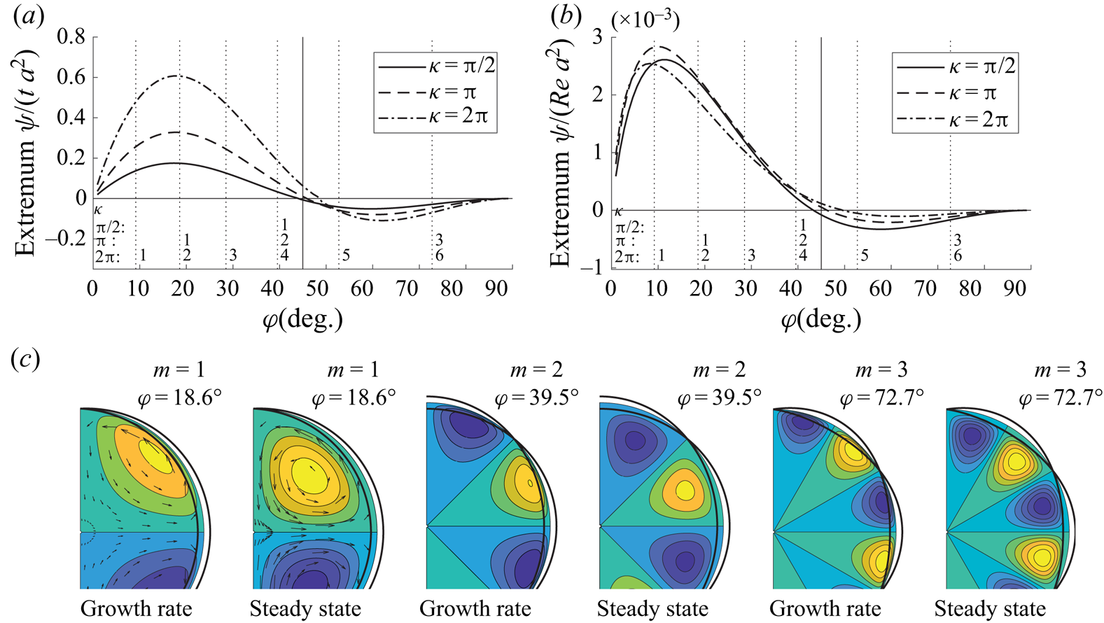
Figure 9. Initial growth rate compared with final steady-state solution. (a) Initial growth rate, inviscid. (b) Ultimate, steady-state solution. (c) Streamlines.


 Open access