
Abstract
The prediction of crack initiation and propagation in ductile failure processes are challenging tasks for the design and fabrication of metallic materials and structures on a large scale. Numerical aspects of ductile failure dictate a sub-optimal calibration of plasticity- and fracture-related parameters for a large number of material properties. These parameters enter the system of partial differential equations as a forward model. Thus, an accurate estimation of the material parameters enables the precise determination of the material response in different stages, particularly for the post-yielding regime, where crack initiation and propagation take place. In this work, we develop a Bayesian inversion framework for ductile fracture to provide accurate knowledge regarding the effective mechanical parameters. To this end, synthetic and experimental observations are used to estimate the posterior density of the unknowns. To model the ductile failure behavior of solid materials, we rely on the phase-field approach to fracture, for which we present a unified formulation that allows recovering different models on a variational basis. In the variational framework, incremental minimization principles for a class of gradient-type dissipative materials are used to derive the governing equations. The overall formulation is revisited and extended to the case of anisotropic ductile fracture. Three different models are subsequently recovered by certain choices of parameters and constitutive functions, which are later assessed through Bayesian inversion techniques. A step-wise Bayesian inversion method is proposed to determine the posterior density of the material unknowns for a ductile phase-field fracture process. To estimate the posterior density function of ductile material parameters, three common Markov chain Monte Carlo (MCMC) techniques are employed: (i) the Metropolis–Hastings algorithm, (ii) delayed-rejection adaptive Metropolis, and (iii) ensemble Kalman filter combined with MCMC. To examine the computational efficiency of the MCMC methods, we employ the \(\hat{R}{-}convergence\) tool. The resulting framework is algorithmically described in detail and substantiated with numerical examples.
1 Introduction
Fracture in the form of evolving crack surfaces in ductile solid materials exhibits dominant plastic deformation. In comparison to brittle materials, the crack evolves at a slow rate and is accompanied by significant plastic distortion. The prediction of such failure mechanisms due to crack initiation and growth coupled with elastic-plastic deformations is an intriguingly challenging task and plays an extremely important role in various engineering applications.
Recently, in the setting of continuum mechanics, a new perspective was proposed for embedding microscopic mechanisms into the macromechanical continuum formulation based on a multi-field incremental variational framework for gradient-extended standard dissipative solids [1, 2]. Typical examples are theories of gradient-enhanced damage [3,4,5,6], phase-field models [7,8,9], and strain gradient plasticity [10,11,12]. Such models incorporate non-local effects based on length scales, which reflect properties of the material micro-structure size with respect to the macro-structure size. In this context, the term size effects is used to describe the influence of the macro-structure size on the mechanical response during inelastic deformations. Thus, micro-structure interaction effects are introduced through the so-called local length-scale, which describes the gradient information of the quantity of interest within neighboring material points (e.g., the damage or ductility zones). From a mathematical point of view, local length-scales resolve the loss of ellipticity of the governing equations and avoid pathological mesh-dependence in post-critical ranges, as well documented in [13,14,15]. Within the variational framework for gradient-extended dissipative phenomena, the modeling challenge is two-fold.
-
First, the derivation of well-posed theoretical formulations for describing the forward model. Hereby, variational phase-field modeling is considered, which is a regularized approach to fracture with a strong capability to simulate complex failure processes. This includes crack initiation (also in the absence of a crack tip singularity) [16,17,18], propagation, coalescence, and branching, without additional ad-hoc criteria [8, 19, 20]. Moreover, the boundary value problem can be solved using standard finite element approximation spaces. A summary of multiphysics phase-field fracture models including algorithmic treatments is outlined in [21]. We further note that, in addition to the finite element method, meshless methods in [22, 23], as well as isogeometric analysis (IGA) in [24] and virtual element method (VEM) in [25] can be used in phase-field models.
-
The second challenge is to elucidate the backward model in order to estimate the model parameters and other univariate quantities of interest. A Bayesian estimation model (as an inverse model) is here used for the ductile fracture problem to provide accurate knowledge regarding the effective mechanical parameters.
1.1 Ductile phase-field fracture as a forward model
A variety of studies have recently extended the phase-field approach to fracture towards the ductile case. The essential idea is to couple the evolution of the crack phase-field to an elasto-plasticity model. Initial works on this topic include [14, 26,27,28,29,30,31,32,33] (see [34] for an overview). Phase-field models for ductile fracture were subsequently developed in the context of cohesive-frictional materials [35, 36], porous plasticity [37] including thermal effects [38], fiber pullout behavior [39], hydraulic fracture [40,41,42], degradation of the fracture toughness [43], multi-surface plasticity [44] and fatigue [45], among others.
The majority of the ductile phase-field models found in the literature are based on local plasticity. In this setting, a strong localization of plastic strains may occur during the post-critical regime, while the damage gradient, as well as the displacement field, suffer jumps [46, 47]. These occurrences are particularly relevant in the case of perfect plasticity due to the absence of a plastic regularization mechanism. Thus, from a numerical perspective, the use of local plasticity in phase-field models does not ensure mesh-objective simulations in the post-critical regime and may lead to non-realistic localized responses, such as ductile fracture with damage growth in non-plasticized regions [48]. To address these problems, phase-field models coupled to gradient-extended plasticity have been proposed in the literature, which incorporate a plastic internal length scale, in the spirit of [49]. The resulting formulation allows for a physically meaningful description of the coupled plasticity-damage evolution and mesh-objective finite element simulations. Models of this class were considered in [45, 50], where a variationally consistent energetic formulation was adopted to derive the coupled system of partial differential equations (PDEs) that governs the gradient-extended elastic-plastic damage response. This approach is consistent with the models proposed in [51] in a finite-strain setting and the extensions to micromorphic regularization [14, 48, 52], where the governing equations were derived from rate-type variational principles, namely, the principle of virtual power.
In this study, we present a unified formulation for ductile phase-field fracture based on variational principles, rooted in incremental energy minimization for gradient-extended dissipative solids [2, 53]. The coupling of plasticity to the crack phase-field is achieved by a constitutive work density function, which is characterized by a degraded stored elastic energy and the accumulated dissipated energy due to plasticity and damage. Three different models are subsequently recovered by certain choices of parameters and constitutive functions. Specifically, two phase-field models coupled to local plasticity are derived, followed by a model that considers gradient extended plasticity. The overall formulation is revisited and extended to the case of anisotropic ductile fracture. Thereby, at a specific material point, the stress state relates to the given direction (resembling solids enhanced with stiff fibers), which entails a deformation-direction-dependent solid material. Hence, similar to [54], a stiffness parameter is introduced to enforce the crack phase-field evolution according to the preferred fiber orientation.
1.2 Bayesian inversion as a backward model
Providing reliable mechanical parameters is essential in computational mechanics to construct models with accurate predictive ability. Many of these a priori unknown parameters cannot be estimated directly through experimental procedures, and a significant effort is often needed to obtain reliable values. Furthermore, material parameters fluctuate randomly in space, giving rise to spatial uncertainty through the geometry. Consequently, the development of a sound statistical framework emerges as an interesting approach to reliably estimate mechanical properties.
Bayesian inversion is a probabilistic technique used to identify unknown parameters. Hereby, a forward model (e.g., a system of PDEs) obtains a set of given data according to the prior density (the initial/prior information of the parameters) and gives a response related to the given unknowns. The output of the inverse problem is the posterior density, which is related to a reference observation (e.g., from experimental or synthetic measurements). This distribution provides very useful information concerning the parameter range, its standard deviation, and expectation.
Markov Chain Monte Carlo (MCMC) methods are frequently employed to extract the posterior distribution of a parameter of interest [55]. We propose several candidates according to the prior density (e.g., uniform/Gaussian) and determine whether the proposed one is rejected or accepted. The Metropolis–Hastings algorithm is one of the most common MCMC techniques due to its efficiency and easiness. In [56], a Bayesian framework according to this algorithm was developed to identify the material parameters in brittle fracture. The method suffers from slow convergence, since most of the candidates are rejected. To enhance its efficiency, several techniques have been recently developed, such as delayed rejection adaptive Metropolis (DRAM) [57], differential evolution adaptive Metropolis (DREAM) [58], and ensemble Kalman filter with MCMC (EnKF-MCMC) [59]. The reader is referred to [56, 60,61,62,63] for the application of Bayesian inversion in applied sciences.
A Bayesian approach (as a backward model) to estimate model parameters for brittle fracture in elastic solids has recently been proposed in [56]. Specifically, the Metropolis–Hastings algorithm is devised therein to approximate model parameters based on synthetic measurements which are obtained through a sufficiently refined discretization space as the replacement of experimental observations. Thereafter, a Bayesian inversion framework for hydraulic phase-field fracture was designed for transversely isotropic and layered orthotropic poroelastic materials [64]. Specifically, the DRAM algorithm was extended for parameter identification.
In this study, we develop a Bayesian inversion framework to identify the effective mechanical parameters in ductile fracture. To this end, we first introduce a methodology to estimate the unknowns in different stages, i.e., elastic, plastic, and fracturing responses for isotropic and anisotropic materials. Three specific MCMC techniques are used to estimate the material parameters using synthetic and experimental measured data. Afterwards, a fair comparison is drawn between two improved models to determine the better convergence rate. As previously mentioned, having accurate information regarding the material parameters will enhance the accuracy of the PDE-based model. For instance, in the present case of ductile fracture, the goal is to predict the dissipative response in different stages, anticipating crack initiation and its propagation during time. We will thus employ the inferred parameters in the model equations and compare the response with the initial knowledge, highlighting the role of the probabilistic approach in improving the model’s performance.


Problem outline and setup of the notation. a Global Cartesian coordinate system with unit vectors \((\varvec{e}_{\varvec{x}},\varvec{e}_{\varvec{y}})\) and local orthogonal principal material coordinates corresponding to the first and second families of fibers \((\varvec{a},\varvec{g})\), b solid with a crack inside of a plastic zone and boundary conditions, and c tangential and unit vectors denoted by \((\varvec{n}_L, \varvec{n}_{\mathcal {C}})\) at the crack tip point \(\varvec{x}\)
1.3 Physical interpretation of the ductile parameters
In ductile fracture, crack propagation is affected by several material properties. Figure 1 shows the range of the different parameters for a wide variety of materials. The effective parameters required in the models are introduced below.
-
The bulk modulus K indicates how much the solid will compress as a result of an applied external pressure, and denotes the relation between a change in pressure and the resulting decrease/increase in fractional volume compression. See, e.g., [65,66,67,68].
-
The shear modulus \(\mu \) is a positive constant, smaller than K, which indicates the response of the solid to shear stress (the ratio of shear stress to shear strain). Large shearing stresses give rise to flow and permanent deformation or fracture. See, e.g., [66, 68, 69].
The elastic properties of the solid can be alternatively described in terms of the Young’s modulus and the Poisson’s ratio, or any other pair of Lamé’s parameters. In our previous work [56], it was reported that due to the boundness of the Poisson’s ratio (\(-1<\nu <\frac{1}{2}\)) and Lamé’s first parameter (\(\lambda >\frac{2\mu }{3}\)), the Poisson’s ratio and Lamé’s first parameter are not appropriate for Bayesian inference. Hence, for the elasticity identification, K and \(\mu \) are selected, where \(K>0\) and \(\mu >0\).
-
The Griffith’s energy release rate \(G_c\) indicates the necessary energy (absolutely positive) to drive crack growth in elastic media. It measures the amount of energy dissipated in a localized fractured state, and therefore has units of energy per unit area. The energy rate is directly related to the toughness, indicating that in tougher materials, more energy is required to initiate fracture [70,71,72].
-
The hardening modulus H characterizes the resistance of the material during plastic deformation. Hardening has an essential impact on crack initiation, specifically in phase transition zones [73]. See, e.g., [74, 75].
-
The yield stress \(\sigma _Y\) denotes the stress related to the yield point (the starting point of plasticity) where the material starts to deform in the plastic regime [69].
-
The critical value \(\alpha _{\mathrm{crit}}\) stems from a physical assumption that fracture evolution is promoted once a threshold value for the accumulated plastic strain has been reached [72].
-
The specific fracture energy \(\psi _c\) characterizes the dissipated energy during a complete damage process in a homogeneous volume element [76]. This property is related to Griffith’s energy release rate and can be interpreted as the amount of strain energy density (strain on a unit volume of material) that a given material can absorb before it fractures [77].
In Sect. 3.4, the role of these quantities in different stages of the deformation process will be clarified.
The paper is structured as follows.
In Sect. 2, a unified version for ductile phase-field fracture models is presented in a variational setting, making use of incremental energy minimization. In Sect. 3, we first introduce the MCMC techniques and explain the three specific Bayesian estimation methods. Afterwards, a parameter identification setting for ductile fracture is presented based on MCMC. Thereafter a review of different possibilities (specific observations) for the implementation of the Bayesian inversion framework is introduced. In Sect. 4, we employ the presented techniques to precisely estimate the effective parameters in different stages of the deformation process. This information allows us to enhance the accuracy of the models, as evidenced by very good agreements between simulations and experiments, highlighting the noticeable efficiency of the MCMC techniques. Furthermore, a fair comparison between the proposed models is outlined. Finally, the conclusions are drawn in Sect. 5.
2 Phase-field modeling of ductile fracture in anisotropic elastic-plastic materials
In this section, we summarize the material models considered for the phase-field approach to ductile fracture. Three models found in the literature are revisited and extended to anisotropic fracture, considering the case of transversely isotropic materials. To this end, a unified formulation is first provided in Sects. 2.1–2.3. The three examined models are then recovered in Sects. 2.4.1–2.4.3. These models will be analyzed in subsequent sections using Bayesian inversion techniques, aiming for parameter identification in anisotropic elastic-plastic fracturing materials.
2.1 Basic continuum mechanics
Let \({\mathcal {B}}\subset {\mathbb {R}}^{\delta }\) be an arbitrary solid domain, \(\delta \in \{2,3\},\) with a smooth boundary \(\partial {\mathcal {B}}\) (Fig. 2). We assume Dirichlet boundary conditions on \(\partial _D{\mathcal {B}} \) and Neumann boundary conditions on \(\partial _N {\mathcal {B}} := \Gamma _N \cup {\mathcal {C}}\), where \(\Gamma _N\) denotes the outer domain boundary and \({\mathcal {C}}\in \mathbb {R}^{\delta -1}\) is the crack boundary, as illustrated in Fig. 2b.
The response of the fracturing solid at material points \({\varvec{x}}\in {\mathcal {B}}\) and time \(t\in {\mathcal {T}} = [0,T]\) is described by the displacement field \({\varvec{u}}({\varvec{x}},t)\) and the crack phase-field \(d({\varvec{x}},t)\) as
Intact and fully fractured states of the material are characterized by \(d({\varvec{x}},t)=0\) and \(d({\varvec{x}},t)=1\), respectively. In order to derive the variational formulation, the following space is first defined. For an arbitrary \(A\subset \mathbb {R}^\delta \), we set
We also denote the vector valued space \(\mathbf {H}^1({\mathcal {B}},A):=\left[ \mathrm{H}^1 ({\mathcal {B}},A)\right] ^\delta \) and define
Concerning the crack phase-field, we set
where \(d_n\) is the damage value in a previous time instant. Note that \({\mathcal {W}}^{d}_{d_n}\) is a non-empty, closed and convex subset of \({\mathcal {W}}^{d}\), and introduces the evolutionary character of the phase-field, incorporating an irreversibility condition in incremental form.
Focusing on the isochoric setting of von Mises plasticity theory, we define the plastic strain tensor \({\varvec{\varepsilon }}^p({\varvec{x}},t)\) and the hardening variable \(\alpha ({\varvec{x}},t)\) as
where \(\mathbb {R}^{\delta \times \delta }_{\mathrm{dev}} :=\{{\varvec{e}}\in \mathbb {R}^{\delta \times \delta } \ :\ {\varvec{e}}^T={\varvec{e}},\ \mathrm{tr}{[{\varvec{e}}]}=0\}\) is the set of symmetric second-order tensors with vanishing trace. The plastic strain tensor is considered as a local internal variable, while the hardening variable is a possibly non-local internal variable. In particular, \(\alpha \) may be introduced to incorporate phenomenological hardening responses and/or non-local effects, for which the evolution equation
is considered. As such, \(\alpha \) can be viewed as the equivalent plastic strain, which starts to evolve from the initial condition \(\alpha ({\varvec{x}},0) = 0 \). Concerning function spaces, we assume sufficiently regularized plastic responses, i.e., endowed with hardening and/or non-local effects, for which we assume \({\varvec{\varepsilon }}^{p}\in \mathbf {Q}:=\mathrm{L}^2({\mathcal {B}}, \mathbb {R}^{\delta \times \delta }_{\mathrm{dev}})\). Moreover, in view of (6), it follows that \(\alpha \) is irreversible. Assuming in this section the setting of gradient-extended plasticity, we define the function spaces
where \({\mathcal {W}}^\alpha =\mathrm{L}^2({\mathcal {B}})\) for local plasticity, while \({\mathcal {W}}^\alpha =\mathrm{H}^1({\mathcal {B}})\) for gradient plasticity. The hardening law (6) is thus enforced in incremental form by setting \(\alpha \in {\mathcal {W}}^\alpha _{\alpha _n,\,{\varvec{\varepsilon }}^p-{\varvec{\varepsilon }}^p_n}\).
The gradient of the displacement field defines the symmetric strain tensor of the geometrically linear theory as
In view of the small strain hypothesis and the isochoric nature of the plastic strains, the strain tensor is additively decomposed into an elastic part \({\varvec{\varepsilon }}^e\) and a plastic part \({\varvec{\varepsilon }}^p\) as
For simplicity, the anisotropic material is assumed to be strengthened by a single family of fibers, whose direction is described by a unit vector field \({\varvec{a}}\) (Fig. 2). Consequently, the direction-dependent response is characterized by the second-order structural tensor
The introduction of additional preferred directions can be easily incorporated in future work, following, e.g., [78]. The solid \({\mathcal {B}}\) is loaded by prescribed deformations and external tractions on the boundary, defined by time-dependent Dirichlet conditions and Neumann conditions
where \({\varvec{n}}\) is the outward unit normal vector on the surface \(\partial {\mathcal {B}}\). The stress tensor \({\varvec{\sigma }}\) is the thermodynamic dual to \({\varvec{\varepsilon }}\) and \(\bar{{\varvec{\tau }}}\) is the prescribed traction vector. Finally, the stress equilibrium is defined as the quasi-static form of the balance of linear momentum
where dynamic effects are neglected and \(\overline{{\varvec{f}}}\) is a given body force.
2.2 Energy quantities and variational principles
Let \({\varvec{{\mathfrak {C}}}}\) denote the set of constitutive state variables. In the most general setting considered in this study, one has
A pseudo-energy density per unit volume is then defined as \(W:=W({\varvec{{\mathfrak {C}}}})\), which is additively decomposed into an elastic contribution \(W_{elas}\), a plastic contribution \(W_{plas}\), and a (regularized) fracture contribution \(W_{frac}\;\):

We note that W is a state function that contains both energetic and dissipative contributions. With this function at hand, a pseudo potential energy functional can be written as
where \({\mathcal {E}}_{ext}\) denotes the work of external loads:
In variationally consistent models, the governing equations of the fracturing elasto-plastic solid can be derived from knowledge of the energy functional (15) by invoking rate-type variational principles [1, 52] in agreement with the principle of virtual power [79, 80]. In such cases, a global rate potential of the form
is defined, where \({\Phi }_{vis}\) denotes the dissipative power density due to viscous resistance forces. In line with previous works [7], the function
is considered, where \(\eta _f\) and \(\eta _p\) are material parameters that characterize the viscous response of the fracture and plasticity evolutions, respectively. Then, minimization of (17) with respect to \(\dot{{\varvec{u}}}\), the plasticity variables \((\dot{{\varvec{\varepsilon }}}^p,\dot{\alpha })\) subject to the hardening law (6), and the crack phase-field \(\dot{d}\) subject to the irreversibility condition \(\dot{d}\ge 0\) provide the governing equations for the elasticity problem, the plasticity problem, and the fracture problem, respectively. Such a variational structure results in a convenient numerical implementation based on incremental energy minimization, for which an algorithmic representation of the energy functional (15) is defined as
where \(\Delta t:=t-t_n\) denotes the time step. The coupled evolution problem then follows as the incremental minimization principle

Remark 2.1
From Eq. (18), it is clear that the rate-independent case is recovered by letting \(\eta _f\rightarrow 0\) and \(\eta _p\rightarrow 0\). In this case, the coupled evolution problem can be equivalently derived in variational form using the energetic formulation for rate-independent systems [81, 82], based on notions of energy balance and stability. This path is followed, for instance, in references [30, 45, 46, 50, 76, 83]. Moreover, the fact that (14) is a state function implies that the incremental rate-independent problem exactly recovers the continuous counterpart.
For the variational formulation setting, it suffices to define the constitutive energy density functions \(W_{elas}\), \(W_{plas}\), and \(W_{frac}\) to establish the multi-field evolution problem in terms of (20). As we shall recall in the sequel, such a variational structure is not always present in phase-field models for ductile fracture, resulting in greater flexibility at the cost of a convenient mathematical structure.
2.2.1 Elastic contribution
The elastic energy density \(W_{elas}\) in (14) is expressed in terms of the effective strain energy density \(\psi _e\). For transversely isotropic materials, \(\psi _e\) is defined in terms of the elastic strain tensor \({\varvec{\varepsilon }}^e\) and the structural tensor \({\varvec{M}}\). In our formulation, in order to preclude fracture in compression, a decomposition of the effective strain energy density into damageable and undamageable parts is employed. Thus, we perform additive decomposition of the strain tensor into volume-changing (volumetric) and volume-preserving (deviatoric) counterparts:
where the volumetric strain is \(\varvec{\varepsilon }^{e,vol}(\varvec{u}) :=\frac{1}{3}(\varvec{\varepsilon }^e(\varvec{u}): \varvec{I})\varvec{I}\) and the deviatoric strain is \(\varvec{\varepsilon }^{e,dev}(\varvec{u}) :=\mathbb {P}:\varvec{\varepsilon }^e\). The fourth-order projection tensor \(\mathbb {P}:=\mathbb {I}-\frac{1}{3} \varvec{I}\otimes \varvec{I}\) is introduced to map the full strain tensor onto its deviatoric component. Therein, \(\mathbb {I}_{ijkl}:=\frac{1}{2}\big (\delta _{ik}\delta _{jl} +\delta _{il}\delta _{jk}\big )\) is the fourth-order symmetric identity tensor.
The effective strain energy density \(\psi _e\) admits the following additive decomposition
The isotropic strain energy function. The isotropic counterpart admits following additive split:
where
where \(I_1\) and \(I_2\) denote the invariants
Accordingly, the isotropic strain energy density function given in (22) is additively decomposed into damageable and undamageable contributions:
where
Therein, \(H{^+}[I_1({\varvec{\varepsilon }}^e)]\) is a positive Heaviside function which returns one and zero for \(I_1({\varvec{\varepsilon }}^e)>0\) and \(I_1({\varvec{\varepsilon }}^e)\le 0\), respectively.
The anisotropic strain energy function. To complete the formulation, the anisotropic strain energy function reads
where the stiffness parameter \(\chi _a\) characterizes the anisotropic deformation response with preferred direction \({\varvec{a}}\). The pseudo-invariant \(I_4\) is defined as
Extending the anisotropic energy into damageable and undamageable parts (see also [64]), the function (27) admits the following split
where
with the Macaulay bracket \(\langle x \rangle _{\pm } := (x \pm \vert x\vert )/2\).
The total elastic strain energy function. The elastic contribution to the pseudo-energy density (14) finally reads
where \(g_e(d,\alpha )\) is the elastic degradation function.
Following the Coleman-Noll procedure, the stress tensor is obtained from the potential \({W}_{elas}\) in (31) as
where \(\widetilde{\varvec{\sigma }}^{iso}\) and \(\widetilde{\varvec{\sigma }}^{aniso}\) are the effective stress tensors, given by
2.2.2 Fracture contribution
The phase-field contribution \(W_{frac}\) is expressed in terms of the crack surface energy density \(\gamma _l\) and the fracture length-scale parameter \(l_f\) that governs the regularization. In particular, the sharp-crack surface topology \({\mathcal {C}}\) is regularized by a functional \({\mathcal {C}}_l\), as outlined in [14, 84] and [53]. This geometrical perspective is in agreement with the framework of [85], which was conceived as a \(\Gamma \)-convergence regularization of the variational approach to Griffith fracture [86]. For the case of isotropic materials, the regularized functional reads
In this work, following [54, 64, 87], anisotropic effects are introduced by means of the structural tensor \({\varvec{M}}\). In particular, we assume that \(\gamma _l\) admits the additive decomposition
In line with standard phase-field models, a general surface density function for the isotropic part \(\gamma _l^{iso}\) is defined as
where \(\omega (d)\) is a monotonic and continuous local fracture energy function such that \(\omega (0)=0\) and \(\omega (1)=1\). A variety of suitable choices for \(\omega (d)\) are available in the literature [88,89,90]. Here, the widely adopted linear and quadratic formulations are considered, which yield, respectively, models with and without an elastic stage. Specifically, we define
On the other hand, the anisotropic part \(\gamma _l^{aniso}\) reads
Finally, the fracture contribution to the pseudo-energy density (14) reads
where \(g_f\) is a parameter that allows to recover different models found in the literature, as will become apparent in the sequel.
2.2.3 Plastic contribution
The plastic contribution \(W_{plas}\) is expressed in terms of an effective plastic energy density \(\psi _p\), whose form will depend on the adopted phenomenological model. In line with previous works [45, 48, 50], let us consider a function in the context of gradient-extended von Mises plasticity:
with the initial yield stress \(\sigma _Y\), the isotropic hardening modulus H and the plastic length-scale \(l_p\). The plastic contribution to the pseudo-energy density (14) then reads
where \(g_p(d)\) is the plastic degradation function. The models presented in Sects. 2.4.1 and 2.4.2 are restricted to local plasticity, for which \(l_p=0\), while the model presented in Sect. 2.4.3 will include non-local effects, with \(l_p>0\). For a variational treatment, it is convenient to invoke the energetic-dissipative decomposition of the plastic energy (41). Thus, the plastic energy density can be further decomposed as
We note that both the isotropic hardening term and the non-local term have been assigned to the free energy density \({W}_{plas}^{ener}\), while the term \(g_p(d)\sigma _Y\alpha \) is viewed as dissipated energy. This distinction is made in agreement with the interpretation of the non-local hardening contribution as a defect energy, as thoroughly discussed in [91]. The role of the decomposition (42) will become clear in Sect. 2.3.3, where the plasticity evolution problem is recovered in variational form.
2.3 Stationarity conditions and governing equations
Let us now derive the variationally consistent equations for the multi-field coupled problem. To this end, we seek to find the stationarity conditions for the minimization problem (20). The models presented in Sects. 2.4.1–2.4.3 shall take the developments below as canonical forms, and will then deviate from the variationally consistent expressions in favor of greater flexibility.
2.3.1 Elasticity
The minimization with respect to the displacement field in the variational principle (20) yields
which corresponds to the weak form of the mechanical balance equations (11), and \({\mathcal {W}}_0^{{\varvec{u}}}\) denotes the function space for the virtual displacement fields, i.e., with homogeneous kinematic boundary conditions.
2.3.2 Fracture
The directional derivative of (15) with respect to the crack phase-field can be written as
where the indicator function \(I_+:\mathbb {R} \rightarrow \mathbb {R} \cup \{+\infty \}\) has been introduced to impose the irreversibility condition embedded in \(d\in {\mathcal {W}}^d_{d_n}\). Let us now define the fracture yield function
The strong form of (44) can then be written as
Recalling that
the strong form yields, for the rate-dependent case, the evolution equation
On the other hand, for the rate-independent case, we obtain the KKT conditions
The main challenge in solving this evolution problem lies on imposing the irreversibility condition \(d\ge d_n\), which allows to replace the set-valued expressions (44) or (46) by equalities. Several alternatives are available in the literature to tackle this problem, including simple penalization methods [92], augmented Lagrangian penalization [93], the primal-dual active set method [94], interior point methods [95], and the complementary system with Lagrange multipliers [96]. In this work, we employ the maximum crack-driving state function method based on the history field, as outlined in [53, 97] and related works.
2.3.3 Plasticity
The three models considered in this study employ von Mises plasticity in the rate-independent case, such that \(\eta _p=0\) in (17). Moreover, as will become clear, the plasticity problem does not follow from the incremental minimization problem (20) in all three models. In particular, a variational formulation for the plasticity problem that is consistent with the governing equations is only possible if the elastic degradation function introduced in (31) does not depend on the hardening variable \(\alpha \), that is, \(g_{e}:=g_e(d)\), such that \({W}_{elas}:={W}_{elas} ({\varvec{\varepsilon }},{\varvec{\varepsilon }}^p,d;{\varvec{M}})\). Let us now summarize the variational formulation of such a model in the general gradient-extended case. A free energy density function for ductile phase-field fracture can be defined as
Applying the Coleman-Noll procedure to the free energy density function (50) yields the following thermodynamic conjugate variables:
In agreement with the classical setting of elasto-plasticity, the yield function is defined as
With the yield function at hand, the strong form of the evolution problem follows from the principle of maximum plastic dissipation
where \(\Phi _p\) is the plastic dissipation potential. The Euler equations of the maximization principle (53) follow as the flow rule and hardening law
together with the KKT conditions
Equations (54) and (55) constitute the so-called dual form of the elasto-plastic problem in strong form. To arrive at a primal formulation, the dissipation potential is evaluated for all \(\dot{\varvec{\varepsilon }}^p \in \mathbb {R}^{\delta \times \delta }_{\mathrm{dev}}\) from (53) as follows (cf. [98, 99]):
Note that in the third line the Cauchy-Schwarz inequality (the upper bound of the second line) is used. Because the sign of \(h^p\) is not a priori specified, the expression inside the supremum is unbounded for \(\dot{\alpha } \ne \sqrt{2/3} \, \vert \dot{\varvec{\varepsilon }}^p\vert \). We can thus write (56) as
Note that by enforcing the hardening law, the time integral of (57) yields the plastic dissipated energy in (42). The Legendre transformation of \(\Phi _p\) then reads
which yields, as a necessary condition, the primal representation of the plasticity evolution problem in the form of a Biot-type equation:
From standard arguments of convex analysis [98, 100], this expression implies the associative flow relations (54) as well as the loading/unloading conditions (55).
To derive the above governing equations from the incremental minimization problem (20), we make use of equations (42) and (57), such that the functional derivative of (19) with respect to \(\{{\varvec{\varepsilon }}^p,\alpha \}\) can be written as
In view of equations (50) and (51), the strong form of (60) can be written as
Equation (61) represents an incremental version of the compact evolution equation (59) for the plasticity model, recovered in a variationally consistent manner from the incremental minimization principle (20). Recall that in the present formulation, this was achieved by assuming an elastic degradation function that does not depend on the plastic variables.
2.4 Specific models revisited
In this section, three benchmark phase-field models for ductile fracture, hereinafter labeled \({\mathcal {M}}_1\), \({\mathcal {M}}_2\), and \({\mathcal {M}}_3\), are revisited within the framework elaborated in the previous sections. The material parameters and constitutive functions that allow to recover each model from the general formulation are presented in Table 1.
2.4.1 Local plasticity with \(G_c\) based fracture criterion: Model 1 (\({\mathcal {M}}_1\))
The first model considered in this study takes the work from [29] as a point of departure. Therein, an extension of the model proposed in [28] was considered by further coupling the fracture process to plasticity through dependence of the elastic degradation function on the hardening variable \(\alpha \). The model was subsequently extended to finite strains and presented with experimental verification in [72]. As discussed in Sect. 2.3.3, dependence of the elastic degradation function on \(\alpha \) results in lack of variational consistency for the plasticity evolution problem, in favor of greater flexibility. In this case, consider the
and the
With the constitutive choices shown in Table 1 for \({\mathcal {M}}_1\), the following specific forms of the governing equations presented in Sect. 2.3 are obtained.
The strong form of the crack phase-field evolution (46) takes the form
Herein, \(\alpha _{\mathrm{crit}}\) is a threshold material parameter introduced in [29] to calibrate the softening response. To enforce the crack irreversibility condition, and, therefore, to cast this inequality constrained boundary value problem (BVP) as an equality constrained BVP, the history field
is introduced. Here, \(\zeta \ge 0\) is a scaling parameter that introduces further flexibility in the formulation, allowing us to tune the post-critical range (cf. [14]). Equation (64) is then restated as
With the last expression, and in view of (43), the global primary fields are found as the solution of the following coupled problem: find \({\varvec{u}}\in {\mathcal {W}}^{{\varvec{u}}}_{\overline{{\varvec{u}}}}\) and \(d\in {\mathcal {W}}^{d}\) such that

Thus,

Remark 2.2
The introduction of the history field in the displacement Euler-Lagrange equation (64), finally yielding (\({\mathcal {M}}_1\)), results in a loss of variational consistency with respect to the energy functional (19) due to the filtering of the maximum history value of \(\widetilde{D}\) and the scaling factor \(\zeta \) for \(\zeta \ne 1\). The upside of this choice is a convenient numerical strategy for solving the original inequality-constrained PDE, and greater flexibility in the model.
Remark 2.3
The role of the parameter \(\zeta \), i.e., tuning the post-critical range by scaling the driving force, is already achieved in the present model by means of \(\alpha _{\mathrm{crit}}\). Consequently, \(\zeta =1\) is assumed hereafter for \({\mathcal {M}}_1\).
Remark 2.4
At this point, it is worth noting that the crack driving force in (\({\mathcal {M}}_1\))\(_2\), i.e., \({\mathcal {H}}\), is scaled by the hardening variable \(\alpha \), such that the crack driving force vanishes for \(\alpha \rightarrow 0\). As a consequence, fracture cannot occur outside the ductility zone, and a response corresponding to elastic damage followed by plastic damage is not possible in this model due to the strong coupling between damage and plasticity. For a detailed discussion of different possible elastic-plastic-damage evolutions, see [30].
Concerning the plasticity evolution problem, a variational derivation in the sense of (60) is not possible in the present model due to the dependence of the elastic degradation function \(g_p\) on \(\alpha \). In this case, the local evolution of the plasticity variables \(\{{\varvec{\varepsilon }}^p,\alpha \}\) according to equations (54) and (55) (alternatively, (59) or the incremental form (61) is postulated in a non-variational context. For the present model, the yield function (52) takes the form
2.4.2 Local plasticity with \(\psi _c\) based fracture criteria: Model 2 \(({\mathcal {M}}_2)\)
The second model is based on the geometrically conceived approach to the phase-field modeling of ductile fracture, conceptually based on the local plasticity theory described in [53] and considered in subsequent works [39, 40]. The original model is constructed within a variationally consistent framework, in agreement with the incremental energy minimization principle (20). In this case, consider the
and the
With the constitutive choices shown in Table 1 for \({\mathcal {M}}_2\), the following specific forms of the governing equations described in Sect. 2.3 are obtained.
Letting \(l_d:=\sqrt{2}\,l_f\) (cf. [76]), and after simple manipulations, the strong form of the crack phase-field evolution (46) can be written as (cf. [14, 53]):
where the role of \(\psi _c\) as a specific critical fracture energy density is clearly reflected. To enforce the crack irreversibility condition, and, therefore, to cast this inequality constrained BVP as an equality constrained BVP, the history field
is introduced. Here, the Macaulay bracket denotes the ramp function \(\langle x \rangle :=(x+|x|)/2\). Letting \(\eta _d:=\eta _f/(2\psi _c)\), (70) is restated as
With the last expression, and in view of (43), the global primary fields are found as the solution of the following coupled problem: find \({\varvec{u}}\in {\mathcal {W}}^{{\varvec{u}}}_{\overline{{\varvec{u}}}}\) and \(d\in {\mathcal {W}}^{d}\), such that

Thus,

Note that, in light of Remark 2.2, the introduction of the history field and the scaling parameter \(\zeta \) in (71) results in a loss of variational consistency with respect to the energy functional (19) for the fracture problem.
On the other hand, as opposed to \({\mathcal {M}}_1\), the local plasticity evolution problem in the present model is variationally consistent (see Sect. 2.3.3). The local evolution of the plasticity variables \(\{{\varvec{\varepsilon }}^p,\alpha \}\) according to the evolution equation (61), which represents an incremental, primal version of equations (54) and (55), is then a necessary condition of the minimization principle (20). For the present model, the yield function (52) takes the form
2.4.3 Non-local plasticity with \(w_0\) based fracture criteria: Model 3 (\({\mathcal {M}}_3\))
The third model considered in this study is inspired by the variational phase-field models coupled to gradient plasticity proposed in [14, 53]. The modeling framework adopted therein and in subsequent studies [37, 51, 52] is consistent with the rate-type variational framework of [1]. In the small-strain rate-independent case, similar models were proposed in [33, 45, 50], where a variationally consistent energetic formulation was adopted to derive the governing equations. Consider, in this case, the
and the
representing a combination of a first-order gradient plasticity model and a first-order gradient damage model. With the constitutive choices shown in Table 1 for \({\mathcal {M}}_3\), the following forms of the governing equations described in Sect. 2.3 are obtained.
With a slight change of parameters, the fracture problem in the present model admits the same formulation of \({\mathcal {M}}_2\) in Sect. 2.4.2. In this case, according to Table 1, the strong form of the crack phase-field evolution (46) can be written as:
where \(w_0\) is a critical fracture energy density. One can show the identity of \(w_0=2\psi _c\) holds for brittle fracture, but in the present gradient plasticity model, \(w_0\ne 2\psi _c\) due to the non-local term in \(\psi _p\). Indeed, the main difference of the present model with respect to \({\mathcal {M}}_1\) and \({\mathcal {M}}_2\) is that the plastic free energy \(\psi _p\), defined in (40), is considered here with \(l_p>0\), and thus introduces non-local effects in the fracture driving force. To enforce the crack irreversibility condition, we define the history field
Thus, (76) is restated as
As before, in light of Remark 2.2, the introduction of the history field and the scaling parameter \(\zeta \) in (71) results in a loss of variational consistency with respect to the energy functional (19) for the fracture problem.
On the other hand, As in \({\mathcal {M}}_2\), the plasticity evolution problem for the present model is variationally consistent (see Sect. 2.3.3). Moreover, the problem now includes non-local effects modulated by the plastic length-scale \(l_p>0\), where the yield function (52) reads
To derive the global PDE governing the evolution of the non-local field \(\alpha \), we take the weak form (60) as a point of departure, such that, for \(\vert {\varvec{\varepsilon }}^p-{\varvec{\varepsilon }}^p_n\vert {>}0\):

where \(\hat{{\varvec{n}}}:=({\varvec{\varepsilon }}^p-{\varvec{\varepsilon }}^p_n)/\vert {\varvec{\varepsilon }}^p-{\varvec{\varepsilon }}^p_n \vert \) is the direction of the plastic flow. Note that in (80), we have considered virtual fields
such that the direction of the plastic flow is fixed, while the virtual equivalent plastic strain \(\delta \alpha \in {\mathcal {W}}^\alpha _{0,\,\delta {\varvec{\varepsilon }}^p}\) is allowed to vary. To solve (80), we must enforce the constraint embedded in \(\alpha \in {\mathcal {W}}^\alpha _{\alpha _n,\,{\varvec{\varepsilon }}^p-{\varvec{\varepsilon }}^p_n}\) (Equation (7)), such that
Recalling that (80) is a weak representation of (61) for \(\vert {\varvec{\varepsilon }}^p-{\varvec{\varepsilon }}^p_n\vert >0\), and that (61) implies the incremental version of the plastic flow rule (54), a possible way to proceed is to replace the local field \({\varvec{\varepsilon }}^p\) by setting, in agreement with (54),
where, from standard arguments of von Mises plasticity, \({\varvec{F}}^{p,trial}:={\varvec{F}}^{p}({\varvec{\varepsilon }},{\varvec{\varepsilon }}^p_n,d;{\varvec{M}})\). With this expression at hand, (80) may be left as a function of the non-local field \(\alpha \), subject to the irreversibility condition \(\alpha \ge \alpha _n\).
Finally, the global primary fields are found as the solution of the following coupled problem: find \({\varvec{u}}\in {\mathcal {W}}^{{\varvec{u}}}_{\overline{{\varvec{u}}}}\), \(\alpha \in {\mathcal {W}}^{\alpha }\), and \(d\in {\mathcal {W}}^{d}\), such that

Thus,

Note that in (\({\mathcal {M}}_3\))\(_2\), it is assumed that the plastic strain tensor is given as a function of \(\alpha \) and the trial direction \(\hat{\varvec{n}}^{trial}\). As such, the dependence of the deviatoric stress \(\varvec{F}^{p}\) on the plastic strains can be eliminated via (83), leaving \(\alpha \) as the only primary unknown in the subproblem. To show the consistency of this equation with the governing equations derived in Sect. 2.3.3, we first recall that the incremental flow rule has been enforced by means of (83). Then, we note that the strong form of (\({\mathcal {M}}_3\))\(_2\) yields \(\beta \in \partial _d I_+(\alpha -\alpha _n)\), with \(\beta \) given in (79). In view of (47), it is easy to see that this expression represents the incremental version of the KKT conditions (55). To handle the inequality constraint and eliminate the multivalued term \(\partial _d I_+(\alpha -\alpha _n)\), a constrained optimization technique is required. For instance, an interior-point method has been recently proposed in [95].
In the sequel, the phase-field models for ductile fracture formulated in \({\mathcal {M}}_1\), \({\mathcal {M}}_2\), and \({\mathcal {M}}_3\) will be taken as inputs for the Bayesian inversion framework described in a detail in Sect. 3.
3 Parameter estimation based on Bayesian inference
In this section, we review different parameter estimation techniques based on MCMC to identify the mechanical parameters involved in ductile fracture. First, some basic statistical principals are briefly recalled.
In Bayesian estimation, a parametric forward model (e.g., a PDE-based model or a coupled variational inequality system) is used to update the available data (considered as random variables) based on the available information (prior knowledge). The posterior information is then provided as output [55, 101, 102].
Bayes’ formula prescribes the probability of an event according to related prior information and is given by
where P(A|B) denotes the conditional probability of event A happening when B has happened (likewise for P(B|A)), and \(P(\cdot )\) is the probability of observations A and B. Using a probability density function \(\pi \), we can rewrite (84) as
Here, \(\pi _0(\chi )\) is the prior distribution which indicates the available information regarding the parameter \(\chi \). For the ductile fracture case, the set of parameters \(\chi \) is indicated in (108). Moreover, \(\pi (\chi |m)\) denotes the posterior density, i.e., the probability density of the parameter \(\chi \) considering the measurement m. The probability of the parameter \(\chi \) with respect to the observation/measurement is described by the likelihood function \(\pi (m|\chi )\). The denominator \(\pi (m)\) is a constant normalization factor, such that
Here, the solution of the inverse problem is the posterior density giving the distribution of the unknown parameter values based on the sampled observations. MCMC is a popular method to calculate this distribution, where a Markov chain is constructed whose stationary distribution is the sought posterior distribution in Bayes’ theorem.
In order to identify the unknown parameters, we introduce the following statistical model:
where \(\mathbb {M}\) is an n-dimensional vector that indicates the measurement, f denotes the PDE-based model, and \(\chi =\{\chi _{_1},\chi _{_2}\ldots ,\chi _{_k}\}\) is a k-dimensional vector denoting the model parameters. The model output \(f(\varvec{x},\chi )\) is the response quantity of interest, collected in an n-dimensional vector, where \(n=n_Tn_C\), with \(n_C\) denoting the number of components of the response variable and \(n_T\) denoting the number of time steps. In the present work, the force-displacement curve is taken as the response variable \(f(\chi )\), such that \(n_C=1\). For the measurement error \(\varepsilon \), we employ a Gaussian independent and identically distributed error \(\varepsilon \sim {\mathcal {N}}(0,\sigma ^2\,I)\), where \(\sigma ^2\) is a fidelity parameter, and \({\varvec{I}}\) is an indentity tensor.
Given a measurement or observation \(m=\texttt {obs}\), the conditional density reads
The inverse problem in the Bayesian framework can thus be stated as follows: given a measurement m, find the posterior density \(\pi (\chi |m)\).
To this end, one makes use of Bayes’ theorem of inverse problems [55], which can be stated as follows:
Proposition 1
(Bayes’ theorem for parameter estimation) We consider random parameter variables \(\chi \) and a specific prior distribution \(\pi _0(\chi )\), and we consider m to be a realization of the random observation variable (denoting the measurement). The posterior distribution considering the measurement m follows as
When using the above relation, one implicitly assumes that observed data is used to construct the posterior density. We should note that in our problem of interest, in case that an experimental measurement is not available, a virtual observation \(\texttt {obs}\) resulting from a fine spatial discretization is alternatively employed. Obviously, the observation is more valuable when a real experiment exists.
If we employ the statistical model (87) with the assumption that errors are Gaussian independent and identically distributed and \(\varepsilon _i\sim N(0,\sigma ^2)\), where \(\sigma ^2\) is fixed, then the likelihood function is
where
is the sum of square errors.
Considering the given likelihood function (90), the posterior distribution has the following form:
where \({\mathcal {S}}{\mathcal {S}}_\xi \) is the sum of squares defined by the integration variable; see (91). From a numerical point of view, we can approximate the integral as
where the quadrature points and weights are denoted, respectively, by \(\xi ^i~\text {and}~w^i\).
In statistics, MCMC methods comprise a class of algorithms for sampling from a probability distribution. By constructing a Markov chain with the desired distribution as its equilibrium distribution, one can obtain a sample of the desired distribution by observing the chain after a number of steps. The more steps there are, the more closely the distribution of the sample matches the actual desired distribution.
In Bayesian statistics, the recent development of MCMC methods has been a key step in making it possible to compute large hierarchical models that require integration over hundreds or even thousands of unknown parameters. In rare event sampling, they are also used for generating samples that gradually populate the rare failure region.
Below, different popular MCMC methods are reviewed. These methods will be used to identify the parameters in ductile fracture in Sect. 4. A detailed comparison between the performance of the methods will be given to clarify their efficiency.
3.1 Metropolis and Metropolis–Hasting algorithms
The Metropolis–Hastings (MH) algorithm is one of the most common techniques among the MCMC methods due to its simplicity for implementation and also its ability to handle different scientific/engineering problems (specifically when the parameters are not strongly correlated) [55]. In order to estimate the posterior distribution, in each iteration, a new candidate parameter value is proposed based on the current sample value according to a proposal distribution. Then, the acceptance ratio is calculated to decide whether the candidate value is accepted or rejected. The acceptance ratio points out how probable the new candidate value is with respect to the current sample.
The method was first introduced by Metropolis [103] based on a random walk. The algorithm starts from the initial guess (the prior value) \(\chi ^0\). Afterwards, according to the chosen proposal distribution a new candidate \(\chi ^\star \) is proposed, which possibly depends on the previous candidates. Having the new candidate \(\chi ^{\star }\), the acceptance rate is calculated as
As the next step, a random variable \({\mathcal {R}}\sim \text {Uniform}\,(0,1)\) is produced. If \({\mathcal {R}}<\lambda \) the candidate is accepted; otherwise, we reject the new proposal and keep the previous candidate in the chain. We follow this procedure for a sufficiently high number of replications. As seen, the algorithm is simple and efficient, specifically when a suitable proposal density is chosen and a large sampling is used. However, an inappropriate proposal results in a significant decrease in performance. If the proposal is very large, many of the candidates will be rejected; therefore, a good convergence to the target density (posterior distribution) will not be achieved. In contrast, if the proposal is too narrow, although many of the candidates are accepted, the chain movement is very slow, and many of the targets will not be captured.
In the Metropolis algorithm, a symmetric proposal density \(\phi (\chi ^{\star }|\chi ^{j-1})=\phi (\chi ^{j-1}|\chi ^{\star })\) is assumed. According to this condition, a movement towards the proposed candidate from the current point is equal to a backward movement (from the current candidate to the proposed point). The use of a non-symmetric proposal distribution was proposed as an efficient improvement by Hastings [104]. Considering N number of samples, the algorithm is summarized in Algorithm 1.

We can draw the following conclusions:
-
A proposal \(\chi ^{\star }\) that results in \(\pi (m|\chi ^{\star })>\pi (m|\chi ^{j-1})\) entails a small sum of squared error and thus leads to candidate acceptance.
-
A proposal \(\chi ^{\star }\) that leads to \(\pi (m|\chi ^{\star })<\pi (m|\chi ^{j-1})\) entails a higher sum of squared error and the proposal may be rejected.
Regarding the proposal functions and how they affect the posterior distribution, if the variance is too large, a large percentage of the candidates will be rejected, since they will have smaller likelihoods, and hence the chain will stagnate for long periods. The acceptance ratio will be high if the variance is small, but the algorithm will be slow to explore the parameter space.
There are different measures to determine if the Markov chain is efficiently sampling from the posteriori density. A good criterion is the acceptance rate (the percentage of accepted candidates). The ratio can be used to tune the proposal density, i.e., reduce its variance. Another efficiency test is the autocorrelation function. The lag-\(\tau \) autocorrelation function \(ACF:\mathbb {N}\rightarrow [-1,1]\) is estimated by
Here, \(\chi _j\) denotes the j-th element of the Markov chain and \(\bar{\chi }\) is the mean value. Note that \(ACF(\tau )\) is positive and monotonically decreasing. The interested readers can refer to [56], where the authors studied the effect of ACF on different parameters in phase-field modeling of brittle fracture. A more advanced convergence analysis such as \(\hat{R}\)-statistics can be implemented when multiple MCMCs with different initial values are used. In Sect. 4, we will use such a diagnostic tool to compare the performance of the Bayesian techniques.
3.2 Delayed rejection adaptive metropolis (DRAM)
At this point, it is worth discussing some improvements in the MH algorithm based on the proposal distribution. The main disadvantage of the model is that the covariance of the proposal should be tuned manually. To improve the efficiency, an alternative to using a fixed proposal distribution in each iteration is to update the distribution according to the available samples (adaptive Metropolis). This approach is useful since the posterior distribution is not sensitive to the proposal distribution.
To adapt the proposal function according to the obtained information, Haario et al. [105] proposed a technique where the current point is chosen as the proposal center and the covariance function is updated using the estimated data. To this end, one can use the following proposal estimation
where the parameter \(\epsilon \) is chosen very small (close to zero) and \(S_p=\frac{2.38^2}{j}\) (as the scaling parameter). The covariance function is calculated by
where \(\hat{\chi }^j=\frac{1}{j+1}\sum \nolimits _{i=0}^{j}\chi ^j\) [55]. The proposal adaptation can be done after a specific number of steps (e.g., 1000) instead of all steps. The efficiency of the algorithm can be further enhanced by adding a delayed rejection step. Green and Mira [106] proposed that instead of a rejected candidate, a second stage is used to propose it from another proposal density. As the first step we propose the new candidate using the Cholesky decomposition of the covariance function (97):
where \({\mathcal {U}}\sim \text {Uniform}~(0,I_j)\) and \(I_j\) is the j-dimensional identity matrix. The alternative proposal \(\chi ^{**}\) is chosen using the proposal function
where \(V_j\) is the covariance matrix estimated by the adaptive algorithm [106]. The essential parameter is \(\gamma _2\), which will be chosen less than one so that the next stage has a narrower proposal function (normally, \(\gamma _2=1/5\) is chosen). We use the following acceptance ratio:
Then, similar to the MH algorithm, we follow the Markov chain to accept/reject the candidate. A summary of the process is given in Algorithm 3.
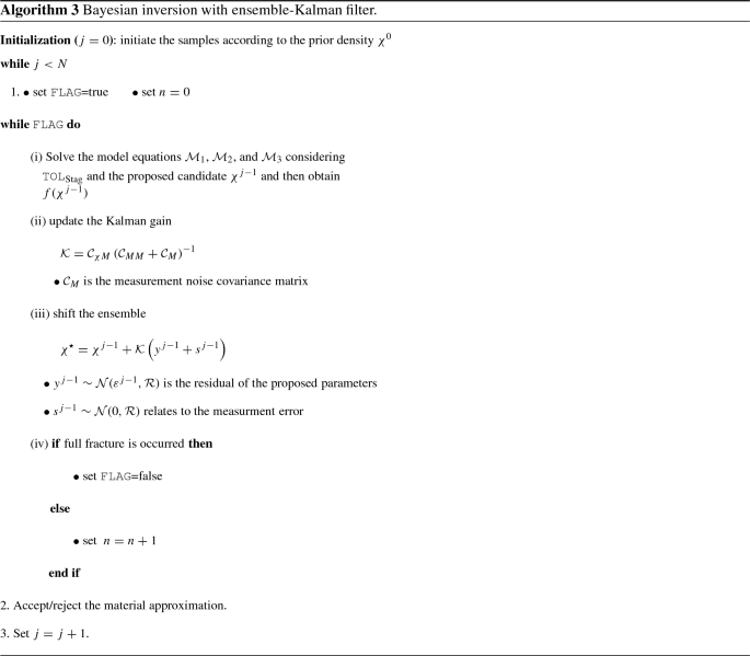
3.3 MCMC with ensemble-Kalman filter
As previously mentioned, a good detection of the proposal density will enhance the Markov chain movement to the target density. Here, we introduce another proposal distribution detection technique using an ensemble-Kalman filter to obtain
where \(\Delta \chi \) denotes the jump of Kalman-inspired proposal. In order to update the proposal, we can separate (100) into
The first term indicates the so-called Kalman gain, i.e.,
where \({\mathcal {C}}_{\chi M}\) is the covariance matrix between the inferred parameters and the PDE-based model, \({\mathcal {C}}_{MM}\) is the covariance matrix of the PDE response, and \({\mathcal {C}}_{M}\) denotes the measurement noise covariance matrix [107]. In (101), \(y^{j-1}\) is the residual of candidates with respect to the model. In other words, considering \(\bar{m}\) an observation/measurement, \(y^{j-1}=\bar{m}-f(\chi ^{j-1})\) and \(s^{j-1}\sim {\mathcal {N}}(0,{\mathcal {R}})\), related to the density of measurement.
Considering the ductile fracture process, crack propagation is modeled until full fracture has occurred. To highlight this procedure, we have added criterion (iv) to Algorithm 3. For the two other algorithms (MH and DRAM techniques), the same condition can be considered.
3.4 Bayesian inversion for ductile phase-field fracture
A proper knowledge about the mechanical parameters that influence the behavior of fracturing solids is crucial to observe the model response and precisely predict crack initiation and propagation during different stages of the deformation process. Bayesian inversion techniques are convenient tools to monitor the crack behavior using observations (e.g., the measured data) and solving the inverse problem considering the forward model (here \({\mathcal {M}}_1\), \({\mathcal {M}}_2\), and \({\mathcal {M}}_3\)). Below, we review different possibilities for the implementation of Bayesian inversion in the context of elastic-plastic fracturing solids governed by phase-field models.
-
Based on the load-displacement curve: this approach allows us to observe the crack behavior in all time steps up to complete failure. At time-step n, the load-displacement curve can be computed as
$$\begin{aligned} F_n=\int _{\partial _D{\mathcal {B}}} \varvec{n}\cdot \varvec{\sigma } \cdot \varvec{n}\,da, \end{aligned}$$(103)where \({\varvec{n}}\) is the outward unit normal on the surface, defined in (11). The main advantage of working with this curve is its easiness, since it involves a one-dimensional parameter. However, it is sensitive to the mesh size and the length scale; therefore, a sufficiently small (and thus more computationally expensive) mesh size is needed.
-
Based on the point-wise primary fields: this approach monitors the crack behavior, the displacement, and the equivalent plastic strain in the entire geometry. Here, the Bayesian setting strives to find the inferred parameters \(\chi ^\star \) which minimize
$$\begin{aligned}&\Vert \bar{\varvec{u}}(\varvec{x})-\varvec{u}(\varvec{x},\chi ^\star ) -\varepsilon _1{\mathcal {I}}\Vert ^2+\Vert \bar{d}(\varvec{x})-d(\varvec{x},\chi ^\star ) -\varepsilon _2{\mathcal {I}}\Vert ^2\\&\quad +\Vert \bar{\alpha }(\varvec{x})-\alpha (\varvec{x}, \chi ^\star )-\varepsilon _3{\mathcal {I}}\Vert ^2, \end{aligned}$$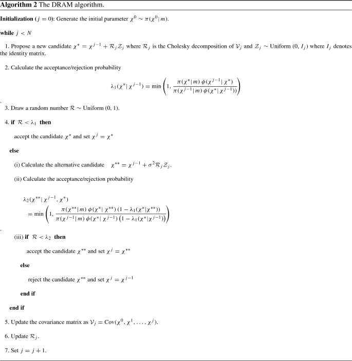
where \(L^2\)-norm can be used, and \(\bar{\varvec{u}}\), \(\bar{d}\), and \(\bar{\alpha }\) are the experimental data throughout geometry with respective measurement errors \(\varepsilon _1\), \(\varepsilon _2\), and \(\varepsilon _3\). This method is informative and provides precise information since the displacement and phase-filed in the entire geometry are considered. However, it is difficult and perhaps even impossible to obtain the measured data from actual experiments in a point-wise manner. Furthermore, a small mesh size must be chosen in numerical simulations to guarantee accurate estimations in the whole geometry, further rendering the method computationally prohibitive.
-
Based on the point-wise phase-field propagation: this approach is less complex than the previous method. Reliable experimental values of the crack path can be obtained using X-ray or \(\mu \)-CT scan in two- or three-dimensional problems; see, e.g., [108]. However, the computational issue regarding mesh sensitivity persists.
-
Based on snapshots of proper orthogonal decomposition (POD): this approach employs a reduced order method (ROM) to reduce the computational complexity. Here, the snapshots of the solution (using measurements of the crack phase-field) are used to construct the POD basis [109]. If an efficient ROM is used, the computational complexity can be reduced significantly. Similarly, a Global-Local approach [110] can be employed to reduce the computational complexity of the forward model.
-
Based on the effective stress-strain response: this approach explains the relation between \(\varvec{\varepsilon }\) and \(\varvec{\sigma }\). It provides useful information regarding different material properties such as bulk modulus, hardening, and yield strength. Therefore, considering the availability of measurements, it entails an instructive procedure. Nevertheless, the computational costs, i.e., the effect of the mesh size and length scale, must be taken into account.


In this work, we choose the load-displacement curve as the observation, and sufficiently small mesh sizes are used to model the crack propagation. Nevertheless, it is worth noting that POD-ROM approaches have significant simulation advantages (noticeable computational cost reduction), while methods based on the stress-strain response are very informative. These procedures will be addressed in future works.

Step-wise Bayesian inversion method to determine the posterior density of the material unknowns for ductile phase-field fracture models
Now, we proceed to establish a Bayesian inversion (\(\texttt {BI}\)) setting to identify the different parameters in ductile fracture. Let us assume that the response of ductile phase-field fracture is either elastic, followed by elastic-plastic, followed by elastic-damage (hereafter \(\texttt {E-P-D}\)); or elastic, followed by elastic-plastic, followed elastic-plastic-damage (hereafter \(\texttt {E-P-DP}\)). Next, we aim at determining the candidate \(\chi \in (\mu ,K,H,\sigma _Y,\psi _c,G_c,w_0,l_p)\) as follows:
-
(1)
To find \(\tilde{\mu }\) and \(\tilde{K}\), we set \(H^0\rightarrow \infty \), \(l^0_p\rightarrow 0\) (in case of \({\mathcal {M}}_3\)), \(\chi ^0_a\rightarrow 0\) (in the anisotropic case), and \(G^0_c\rightarrow \infty \) in \({\mathcal {M}}_1\), \(\psi ^0_c\rightarrow \infty \) in \({\mathcal {M}}_2\), and \(w^0_0\rightarrow \infty \) in \({\mathcal {M}}_3\), thus reflecting an elastic response. We then have
$$\begin{aligned} (\tilde{\mu },\tilde{K})=\texttt {BI}\,(\mu ^0,K^0,\sigma _Y^0,H^0,l^0_p,G^0_c, \psi ^0_c,w^0_0,\chi ^0_a). \end{aligned}$$(104) -
(2)
To find \(\tilde{\sigma _Y}\), we set \(H^0\rightarrow 0\), \(l^0_p\rightarrow 0\) (in case of \({\mathcal {M}}_3\)), \(\chi ^0_a\rightarrow 0\) (in the anisotropic case), and \(G^0_c\rightarrow \infty \) in \({\mathcal {M}}_1\), \(\psi ^0_c\rightarrow \infty \) in \({\mathcal {M}}_2\), and \(w^0_0\rightarrow \infty \) in \({\mathcal {M}}_3\), thus reflecting an ideal plastic response. We then have
$$\begin{aligned} \tilde{\sigma _Y}=\texttt {BI}\,(\tilde{\mu },\tilde{K},Y^0_0,H^0,l^0_p, G^0_c,\psi ^0_c,w^0_0,\chi ^0_a). \end{aligned}$$(105) -
(3)
To find \(\tilde{l_p}\) (in case of \({\mathcal {M}}_3\)) and \(\tilde{H}\), we set \(\chi ^0_a\rightarrow 0\) (in the anisotropic case), \(G^0_c\rightarrow \infty \) in \({\mathcal {M}}_1\), \(\psi ^0_c\rightarrow \infty \) in \({\mathcal {M}}_2\), and \(w^0_0\rightarrow \infty \) in \({\mathcal {M}}_3\), thus reflecting an elastic-plastic response prior to fracture. We then have
$$\begin{aligned} (\tilde{H},\tilde{l_p})=\texttt {BI}\,(\tilde{\mu },\tilde{K}, \tilde{\sigma _Y},H^0,l^0_p,G^0_c,\psi ^0_c,w^0_0,\chi ^0_a). \end{aligned}$$(106) -
(4)
To find \(\tilde{\chi _a}\) (in the anisotropic case), \(\tilde{G_c}\) in \({\mathcal {M}}_1\), \(\tilde{\psi _c}\) in \({\mathcal {M}}_2\), and \(\tilde{w_0}\) in \({\mathcal {M}}_3\), which reflect a ductile anisotropic fracture response, we have
$$\begin{aligned} (\tilde{G_c},\tilde{\psi _c},\tilde{w_0},\tilde{\chi _a}) =\texttt {BI}\, \left( \tilde{\mu },\tilde{K},\tilde{\sigma _Y}, \tilde{H},\tilde{l_p},G^0_c,\psi ^0_c,w^0_0,\chi ^0_a\right) . \end{aligned}$$(107) -
(5)
Finally, we obtain the following parameter estimation:
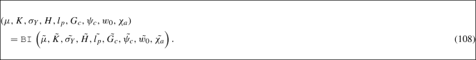

Figure 3 shows the overall procedure, indicating all stages of the deformation process. Note that, from the implementation point of view, we set the limit \(\infty \) as \(10^8\times E\), where E refers to Young’s modulus, while the lower limit is set to 0. From the statistical point of view, we employ the MCMC techniques (Algorithms 1–3) to identify the parameters in Step (1); then, we follow Step (2) to estimate \(\sigma _Y\) and pursue the parameter identification procedure until we determine the whole set of material parameters in Step (4).
In a similar manner, if the response is elastic, followed by elastic-damage, followed by elastic-plastic-damage, i.e., \(\texttt {E-D-PD}\) (see [30] for a detailed discussion on different possible evolutions), we first determine the elastic moduli, followed by the anisotropic fracture properties by assuming that the response is brittle, and finally, we determine the plastic proprieties in the final dissipative stage.
Regarding parameter correlations, we note that the effective bulk modulus \(K=\lambda + \frac{2\mu }{3}\) and the shear modulus \(\mu \) are chosen as the elasticity parameters. This relation points out that \(\mu \) and K are fully correlated which should be considered in the posterior density. Moreover, the critical energy release rate \(G_c\) is directly correlated to the specific fracture energy. These considerations will be taken into account in the Bayesian inversion.
4 Numerical examples
This section demonstrates the performance of the proposed Bayesian inversion approaches for parameter estimation within the ductile phase-field fracture models presented earlier. We investigate four numerical examples. To validate the numerical method, the last two examples are concerned with experimental observations, in which the posterior responses are compared with experimental load-displacement curves. The material parameters listed in Table 2 are considered, which are initialized based on [29, 72]. In the MCMC the observational noise \(\sigma ^2=10^{-3}\) is used.
Space discretization In the numerical simulations, the global primary variables are discretized using finite element basis functions, with bilinear quadrilateral \(Q_1\) elements for the two-dimensional problems and trilinear hexahedral \(H_1\) elements for the three-dimensional problems.
Solution of the nonlinear problems A staggered scheme is used for solving the variational equations resulting from the ductile phase-field fracture models (Sect. 2.4). For model 1 \(({\mathcal {M}}_1)\) and model 2 \(({\mathcal {M}}_2)\), we alternately solve for \(d/{\varvec{u}}\) by fixing \({\varvec{u}}/d\) until convergence is reached. Accordingly, for model 3 \(({\mathcal {M}}_3)\), we alternately solve for \({\varvec{u}}\) by fixing \((\alpha ,d)\), and then solve for \(\alpha \) by fixing \((\varvec{u},d)\). Next, we obtain the plastic strain tensor \({\varvec{\varepsilon }}^p\) though the incremental plastic evolution equation (82), and lastly, we find d by fixing \((\varvec{u},\alpha )\), repeating the procedure until convergence is reached.

Geometry and boundary conditions of the I-shaped tensile specimen: a Example 1, and b Example 2
At this point, it is necessary to remark on the convergence criteria for the staggered scheme. Let n and k represent the loading time step and iteration counter, respectively. At the fixed loading time step n, we obtain a converged state if the following holds:
Additionally, an iterative Newton solver is used in which the individual nonlinear equation systems are solved. The stopping criterion of the single scale and local Newton methods is \(\texttt {Tol}_{\texttt {N-R}}=10^{-10}\). Specifically, the relative residual norm is given by \(\texttt {Residual}: \Vert \varvec{F}(\varvec{x}_{k+1}) \Vert \le \texttt {Tol}_{\texttt {N-R}} \Vert \varvec{F}(\varvec{x}_{k}) \Vert \). Here, \(\varvec{F}\) refers to the residual of the discretized equilibrium equation of the nonlinear BVPs. The interested reader can refer to [111,112,113,114,115,116,117] for the developed linear/nonlinear solvers for phase-field fracture.
4.1 Example 1: Asymmetrically I-shaped specimen under tensile loading
To gain a first insight into the performance of the Bayesian inversion approach, the following numerical example is concerned with the asymmetrically notched I-shaped specimen under tension. The configuration is shown in Fig. 4a. The geometrical dimensions are set as \(H_1=110\ \hbox {mm}\), \(H_2=25\ \hbox {mm}\), \(r_1=3.625\ \hbox {mm}\), \(w_1=22\ \hbox {mm}\), and \(w_2=14.8\ \hbox {mm}\), with half-circular notches of radius \(r_2=2.5\ \hbox {mm}\). The two notches are placed at a vertical distance from the center of \(10\ \hbox {mm}\).
A monotonic displacement increment \({\Delta \bar{u}}_y=2\times 10^{-3}\ \hbox {mm}\) is applied in the vertical direction at the top boundary of the specimen. The minimum finite element size in the domain is \(0.3\ \hbox {mm}\), for which the heuristic requirement \(h<l/2\) inside the localization zone is fulfilled. Consequently, the I-shaped domain partition contains 21598 elements. The material and numerical parameters are given in Tables 2 and 3, respectively.

Example 1: the effect of all studied parameters on the load-displacement curve. Here, we depict the curves obtained by \({\mathcal {M}}_1\) for \(\mu \), K, H, \(\sigma _Y\), \(\alpha _{\mathrm{crit}}\), \(G_c\) (the first and the second row). In the third row, we depict the effect of \(\psi _c\) (\({\mathcal {M}}_2\)) as well as \(\zeta \) and \(w_0\) (\({\mathcal {M}}_3\))

Example 1: the posterior distribution of the effective parameters using \({\mathcal {M}}_1\), \({\mathcal {M}}_2\), and \({\mathcal {M}}_3\)
For all three models, the shear modulus \(\mu \), the bulk modulus K, the hardening modulus H, and the yield stress \(\sigma _Y\) are common. First, we study the effect of the common parameters on the load-displacement curve. Figure 5 shows the diagrams where \({\mathcal {M}}_1\) is used to obtain the solutions. To monitor different critical values \(\alpha _{\mathrm{crit}}\) and energy release rates \(G_c\), as well as fracture energies \(\psi _c\), \({\mathcal {M}}_1\) and \({\mathcal {M}}_2\) are respectively employed. Moreover, we used \({\mathcal {M}}_3\) to observe how the curve is affected by specific values of \(w_0\) and the parameter \(\zeta \), as shown in Fig. 5.


Example 1: the load-displacement curve for the inferred equivalent values \(\psi _c\), with \(\psi _c\) varying between 25 and 65

Example 1: approximated solution obtained through the posterior density of the material parameters at complete failure. The hardening value \(\alpha \) and the crack phase-field d are shown for different models
Next, we proceed to identify the effective parameters in the ductile fracture process using the Metropolis–Hastings algorithm introduced in Section 3.1. The Bayesian framework for ductile fracture is presented in Section 3.4. We employ a uniform distribution to estimate the parameters more accurately, as listed in Table 3 (the prior densities and the initial values) and use \(N=10\,000\) number of candidates. Regarding the reference values, a synthetic measurement is used, using a total number of degrees of freedom \({\mathcal {N}}_{\mathrm{dof}}=28\,380\); the rest of the initial values are summarized in Table 3. The posterior density of the parameters using the three models is shown in Fig. 6. The mean values of the posterior distributions are used to verify the parameter estimation. The inferred information is listed in Table 4. To verify the accuracy of the data, we employ the parameters in all three models and compute the load-displacement curve until the fracture point. Figure 7 shows the curves resulting from the different models and the reference observation. An excellent agreement indicates that the Bayesian inversion framework identified the parameters correctly, showing a consistent behavior for all three models in all stages.
The accuracy of the Bayesian inversion for all models enables us to provide equivalence for the model parameters. As previously mentioned, all models have four common parameters, but each model is also characterized by its own features. Here, we strive to find an equivalent value for different fracture energies. This allows us to use \({\mathcal {M}}_1\) and \({\mathcal {M}}_3\) and derive similar quantities in \({\mathcal {M}}_2\), and vice versa. To that end, we select the diagram estimated by \({\mathcal {M}}_2\) as the reference observation, where all parameters are chosen according to the estimated values (see Table 4). However, \(\psi _c\) varies between 25 and 65. We again use the MH algorithm to identify the equivalence of \(\psi _c\) in \({\mathcal {M}}_1\) (i.e, \(G_c\) and \(\alpha _{\mathrm{crit}}\)) and \({\mathcal {M}}_3\) (i.e., \(l_p\) and \(w_0\)). The estimated quantities are summarized in Table 5. Figure 8 presents the results obtained by the inferred values, where, again, Bayesian inversion provides a very good agreement.
The resulting equivalent plastic strain (\(\alpha \)) and crack phase-field (d) at complete failure are shown in Fig. 9. The solutions are based on the posterior density of the material parameters for different models, which are given in Table 4. Accordingly, the fracture path initiates within the maximum equivalent plastic regions, which appear near the notches. Next, the crack propagates in the plastic localization band, in which two cracks merge at the specimen center. It can be observed that even though the load-displacement curves shown are practically identical in all models, the corresponding phase-field profiles, and thus, hardening profiles, are not; see Fig. 9. This can be explained, first of all, by the solution non-uniqueness of the phase-field fracture problem, and, secondly, by the fact that the different phase-field models in fact provide only the approximation of the fracture problem. Thus, the necessity of comparing the results with an experimental observation is crucial. Hereby, based on the experimental test provided in [72] (second experiment), a sharp crack transition between two notches is expected. Thus \({\mathcal {M}}_2\) and \({\mathcal {M}}_3\) seem to yield a more accurate fracture pattern.
4.2 Example 2: I-shaped tensile specimen for anisotropic ductile fracture
The main objective of this example is the adoption of Bayesian inversion for an anisotropic ductile phase-field fracture process. The BVP depicted in Fig. 4b consists of an I-shaped specimen with a circular void in the center of the domain. The geometrical dimensions in Fig. 4b are set as \(H_1=110\ \hbox {mm}\), \(H_2=28.6\ \hbox {mm}\), \(w_1=22\ \hbox {mm}\), and \(w_2=14.8\ \hbox {mm}\), with the central void located in \((x,y)=(H_1/2,w_1/2)\), with a radius of \(r=2.5\ \hbox {mm}\).
Herein, we assume that the material constituents are not distributed uniformly through the continuum domain, and thus, the material is divided into several phases. Hence, heterogeneity in strength from one area of the domain to another one is expected. Note, however, that by means of the Bayesian inversion framework, we aim at determining the effective mechanical parameters. So, in our Bayesian inversion calculation a homogeneous response is considered. Here, we consider the parameters as a random field (with given mean and variation). Figure 10 illustrates the fluctuation of different material parameters (on the element-wise basis) with spatial correlation where a 10% variation is included. For instance, for the parameter K, the expectation is assumed as K=75,000 MPa, with a variation between 71,700 MPa and 78,800 MPa. This fluctuation will be used to provide the reference observation. Specifically, we will replicate 500 simulations (with a specific mesh size) to estimate the reference observation considering the mentioned variation. The distribution of the parameters on the geometry is shown in Fig. 10.
The numerical example is performed by applying a monotonic displacement increment \({{\Delta \bar{u}}_y}=2\times 10^{-3}\ \hbox {mm}\) in the vertical direction at the top boundary of the specimen (Fig. 4). The bottom edge is fixed in the \(x-y\) directions. The minimum finite element size is \(0.45\ \hbox {mm}\). The two-dimensional I-shaped domain partition contains 17038 elements.
In this example, to determine the effective mechanical parameters, the DRAM algorithm is used. Due to the anisotropic structure of the solid, in addition to the identified parameters in Example 1, the stiffness parameter \(\chi _a\) must be estimated. Here, we select a fiber orientation \(\phi =45^o\) for the parameter identification and propose \(N=10\,000\) candidates. A synthetic reference value using \({\mathcal {N}}_{\mathrm{dof}}=26\,870\) is employed as the reference observation considering the already mentioned parameter variation. The prior (uniform) densities of the parameters are listed in Table 6. For each parameter, the inferred values by different models are relatively similar, which highlights the robustness of the Bayesian setting. The posterior distributions are depicted in Fig. 11. The mean values of the posterior distributions are given in Table 7 using \({\mathcal {M}}_1\), \({\mathcal {M}}_2\), and \({\mathcal {M}}_3\). Again, we solve the model equations employing the identified parameters to verify the effectiveness of the Bayesian framework, as shown in Fig. 7 (right). All diagrams show that implementing the DRAM algorithm gives rise to a reasonable agreement between the models and also with respect to the reference observation.

Example 2: material parameters distribution (prior density) on each element of the domain \({\mathcal {B}}\). Note that here, to avoid a strong deviation of the surrounding points due to the random normal distribution of the material properties, one could use an additional random distribution length-scale to achieve mesh objectivity, that is, the so-called heterogeneity length-scale; see [118]. In this study, we have not used a heterogeneity length-scale since we have assumed that the material distribution provides the synthetic observations

Example 2: the posterior distribution of the effective parameters using \({\mathcal {M}}_1\), \({\mathcal {M}}_2\), and \({\mathcal {M}}_3\)
For further investigation of the sensitivity of the inferred parameters obtained through the DRAM algorithm, two additional preferential fiber directions, namely \(\phi =30^o\) and \(\phi =60^o\), are employed. Again, Fig. 12 illustrates the robustness of the Bayesian setting, showing for all models and different orientations a consistent behavior in the in elastic, plastic, and fracture stages. Figure 13 illustrates the crack phase-field solution at complete failure for \(\phi =30^o\), \(\phi =45^o\), and \(\phi =60^o\). Note that the solutions are based on the posterior density of the material parameters, which are given in Table 9. An important observation is that both the equivalent plastic strain and the crack phase-field evolve in the direction of the preferred fiber orientation.
4.3 Example 3: Flat I-shaped Al-5005 test under tensile loading
While synthetic observations have been used so far, the last two examples are concerned with experimental observations to estimate the posterior density of the material unknowns. The following example considers an I-shaped specimen for Al-5005 material under tensile loading. We aim at reproducing the experimentally observed ductile fracture process of the tensile test through the proposed Bayesian inversion framework. The BVP is shown in Fig. 14a. The experimental observations of necking and fracture are shown in Fig. 14c. The geometrical dimensions are set as \(H_1=144\ \hbox {mm}\), \(H_2=27\ \hbox {mm}\), \(H_3=22\ \hbox {mm}\), \(w_1=20\ \hbox {mm}\), \(w_2=12\ \hbox {mm}\), and \(r_1=14\ \hbox {mm}\). The specimen domain has a \(3\ \hbox {mm}\) thickness, as shown in Fig. 14b.
The numerical example is performed by applying a monotonic displacement increment \({\Delta \bar{u}}_y=0.02\ \hbox {mm}\) in the vertical direction at the top boundary of the specimen for 300 time steps. The minimum finite element size is \(1.5\ \hbox {mm}\). The flat I-shaped domain partition contains 3230 hexahedron linear elements.

Example 2: the load-displacement curve obtained by the estimated values for \(\phi =30^o\) and \(\phi =60^o\) and all three models
Both DRAM and ensemble-Kalman filter (EKF) are efficient MCMC techniques and have shown their computational performance reasonably. However, a fair comparison can determine which method will be more advantageous in ductile fracture.
4.3.1 Convergence performance of the MCMC methods
In the already mentioned examples, the MCMC techniques have been used to identify the mechanical parameters. The main advantage of the MH algorithm is its ease of implementation. However, it suffers from slow convergence, and the starting value may affect the convergence status. The DRAM and EKF variants, as more advanced techniques, show more a productive performance. In this part, we strive to study their efficiency in the context of ductile fracture.
Convergence diagnostics is essential in MCMC methods since it determines the accuracy of the parameter, and with how many iterations the chain converges to the target distribution. Here, we use multiple chains with different initialized values, expecting that a significantly large number of Markov chains give rise to the same results. In other words, the candidate distribution from chains should be similar using multiple initial starting values.
\(\hat{R}\)-convergence diagnostics [119, 120] is an efficient tool to monitor the convergence of the MCMC by comparing the between and within chain estimates for model parameters and other univariate quantities of interest. Assuming m parallel chains, we determine the variance between the chain means B/N and calculate the average of the within chain variances W. The target variance is given by
where N is the length of the chain. Then, we calculate the potential scale reduction factor, or PSRF (also called \(\hat{R}\)-statistics) by
If the MCMC method converges appropriately, the chains are not affected by the starting point, and \(\hat{R}\) reduces to 1. In other words, we can conclude that all chains are close to the target distribution [119]. In order to verify the method efficiency, a threshold can be defined, e.g., values less than 1.5 or 1.2 indicating a good convergence performance.
In the I-shaped example, in order to draw a comparison between DRAM and EKF algorithms, we study their convergence to conclude which model shows a faster convergence taking all inferred parameters into account. We use \(N=1\,000\) and five parallel MCMCs (\(m=5\)) with a uniform distribution indicated in Table 8. Using \({\mathcal {M}}_2\), Fig. 15 shows that by employing EKF in all parameters, fewer candidates are necessary to converge to the posterior density. Indeed, for all parameters excluding K, after \(1\,500\) samples, \(\hat{R}\)- converges to 1, showing a high level of accuracy. The performance of the DRAM is acceptable, since most of the variables after \(2\,500\) samples are below the threshold, although again, the bulk modulus shows more variation (probably due to the large chosen prior density).

Example 2: the crack phase-field at complete failure for all three models. Different preferential fiber directions are considered in the transversely isotropic setting: a \(\phi =30^o\), b \(\phi =45^o\), and c \(\phi =60^o\)

Example 3: flat I-shaped Al-5005 test under tensile loading. a Geometry of specimen with boundary conditions, b three-dimensional perspective, and c experimental observation taken from [72]
According to the above-mentioned discussion, we choose the EKF technique for the rest of the examples. We use five parallel MCMCs with \(2\,000\) samples. For the observation, we use experimental data taken from [72]. Figure 16 shows the posterior density of the estimated parameters, and the mean values are summarized in Table 9. We then employ the identified quantities in all three models. Figure 17 shows a comparison between the load-displacement curve obtained by the models and the experiments. Interestingly, by employing the Bayesian framework, all crack propagation stages (until fracture reaches the boundary) are modeled accurately.
Next, we investigate the ductile failure response employing the posterior density of the material parameters given in Table 9. The evolution of the crack phase-field d is provided in Fig. 17 at three deformation stages up to complete failure. Additionally, the equivalent plastic strain \(\alpha \) at final failure is shown. It can be grasped that, regardless of the formulations, fracture initiation appears at the center of the specimen, and then evolves towards the two edges of the specimen until complete failure. The first important observation is that the simulation results are in good agreement with the experimental failure pattern shown in Fig. 14c. Another important observation is that the crack phase-field in \({\mathcal {M}}_2\) and \({\mathcal {M}}_3\) is more diffuse than \({\mathcal {M}}_1\). The main reason for this is that the crack driving force of \({\mathcal {M}}_1\) is scaled by \(\alpha \); thus, the phase-field diffusivity is strongly coupled to the ductile response; see Remark 2.4.
4.4 Example 4: Sandia fracture challenge
The last example aims at estimating the posterior density of the unknown material properties for a specimen frequently used in the literature, namely, a Sandia fracture challenge [121]. The 2014 fracture challenge problem launched by the Sandia National Lab [121] has provided an ideal platform to assess the computational capability and limitations of each participating team [122]. Specifically, this challenge aims at evaluating the computational ability to predict crack initiation and propagation of ductile fracture with respect to experimental observations. A recent comparative literature overview was conducted in [123]. As reported in [72], standard phase-field formulations without estimating accurate ductile material properties quantitatively overestimate the post-yielding load-displacement response, which can be improved by performing an accurate calibration of the plasticity and phase-field parameters. Hence, we aim at reproducing the experimentally observed Sandia fracture challenge through the proposed Bayesian inversion framework.

The \(\hat{R}\)-statistics test for the convergence of all effective mechanical parameters of the I-shaped example. Here, the DRAM algorithm (left) is compared with EKF (right) using \({\mathcal {M}}_2\). The red dashed line shows a threshold of 1.2

Example 3: the posterior distribution of the effective parameter using \({\mathcal {M}}_1\), \({\mathcal {M}}_2\), and \({\mathcal {M}}_3\)

Example 3: a) the equivalent plastic strain at complete failure, and b the evolution of the crack phase-field for different deformation stages up to final failure at \(\bar{u}_y=6\ \hbox {mm}\)

Example 4: Sandia fracture challenge. a Geometry of specimen with boundary conditions, b three-dimensional perspective, and c experimental observation taken from [72]

Example 4: the posterior distribution of the effective parameters using \({\mathcal {M}}_1\), \({\mathcal {M}}_2\), and \({\mathcal {M}}_3\)
The experiments are based on the material Al-5052 H34, which experimentally induces a complex failure mode; see [70, 72]. The configuration is shown in Fig. 18a, while the experimental observations are shown in Fig. 18c. The geometrical configuration includes two pins. The top pin is displaced vertically, while the lower pin is fixed in all directions. The two pins are considered to be rigid (here taken 10 times stiffer than the rest of the domain). The geometrical dimensions are set as \(H_1=80\ \hbox {mm}\), \(H_2=35\ \hbox {mm}\), \(H_3=15\ \hbox {mm}\), \(H_4=6.5\ \hbox {mm}\), \(w_1=62.5\ \hbox {mm}\), \(w_2=36\ \hbox {mm}\), and \(w_3=12.5\ \hbox {mm}\). The pins have an identical radius of \(r_1=6\ \hbox {mm}\), while the horizontal notch is rounded with a radius of \(r_5=3.25\ \hbox {mm}\). The specimen includes three voids with centers and radii \(c_2=(x_2,y_2)=(27,32)\ \hbox {mm}\) and \(r_2=3\ \hbox {mm}\), \(c_3=(x_3,y_3)=(24,45)\ \hbox {mm}\) and \(r_3=1.75\ \hbox {mm}\), and \(c_4=(x_4,y_4)=(22,38)\ \hbox {mm}\) and \(r_4=1.75\ \hbox {mm}\), respectively. The specimen domain has a \(2\ \hbox {mm}\) thickness, as shown in Fig. 18b.
The numerical example is performed by applying a monotonic displacement increment \({\Delta \bar{u}}_y=0.02\ \hbox {mm}\) in the vertical direction at the top pin for 400 time steps. The minimum finite element size is \(0.32\ \hbox {mm}\). Consequently, the Sandia specimen domain partition contains 17980 hexahedron linear elements.

Load-displacement curve computed using the inferred values, employing \({\mathcal {M}}_1\), \({\mathcal {M}}_2\), and \({\mathcal {M}}_3\). The experimental data are depicted with red. Here, Tables 9 and 11 are used for Example 3 (left) and Example 4 (right). The results are also compared with the simulation results of [72]

Example 4 a The equivalent plastic strain at complete failure, and b the evolution of the crack phase-field for different deformation stages up to final failure at \(\bar{u}_x=8\ \hbox {mm}\). The final fracture stage was not captured with model 2 due to lack of convergence
Due to its efficiency, the EKF technique is again considered for this example to identify the parameters. We use four parallel MCMCs with \(2\,500\) samples. The experimental data (reference observation) is taken from [72] and the prior densities are indicated in Table 10. The posterior distributions are shown in Fig. 19, while the mean values are summarized in Table 11. Finally, once again, we solve \({\mathcal {M}}_1\), \({\mathcal {M}}_2\), and \({\mathcal {M}}_3\) using the inferred values, and compare the results with those obtained in [72]. As shown in Fig. 20, by employing the proposed Bayesian inversion framework, the parameters are estimated accurately, showing very good agreement between the simulated data in all models and the experiments. This implementation also enhanced the computational capabilities of \({\mathcal {M}}_1\), showing an improved model accuracy compared to the results obtained in [72].
For a better insight into the fracture process in all models, the evolution of the crack phase-field d is provided in Fig. 21 at three deformation stages up to complete failure. Additionally, the equivalent plastic strain \(\alpha \) at final failure is shown. Note that the solutions are based on the posterior density of the material parameters, which are given in Table 11.
It can be grasped that, for all three models, the fracture path first initiates at the void located in the middle of the specimen, and afterwards, evolves towards the right edge of the domain. In addition, a secondary crack initiates from the central void, but this time from its left side, and then propagates towards the left edge of the specimen until complete failure. Note further that the simulation results are in good agreement-agreement with the experimental failure pattern shown in Fig. 18c.
Based on our numerical result, it is worth noting that the stage of the secondary crack was no longer predicted by model 2. To estimate the posterior density of the material parameters through Bayesian inversion, several candidates are required. Thus, a stable forward method is crucial. Otherwise, deviating material properties will result in unstable solutions. In this context, we highlight that model 3 provides the most stable solutions, at the cost of an additional PDE that must be solved to obtain the plastic response (as opposed to local plasticity in model 1 and model 2).
5 Conclusion
In this work, we have proposed a robust and efficient step-wise Bayesian inversion method for ductile fracture problems using phase-field models. In particular, a Bayesian inversion framework (the as a probabilistic technique) based on MCMC is developed the to identify unknown ductile fracture parameters. Three common MCMC methods, namely the MH algorithm, the DRAM algorithm, and EKF-MCMC have been used to estimate the effective parameters in ductile fracture. The posterior density results from the inverse problem are evaluated with synthetic measurements (for the first two examples) as well as experimental observations (for the last two examples). To approximate ductile failure, a phase-field fracture formulation is used for a ductile material exhibiting \(J_2\)-plasticity in a quasi-static kinematically linear regime. To do so, we have presented a unified formulation for phase-field modeling of ductile fracture, which is resolved through an incremental energy minimization approach. The overall formulation is revisited and extended to the case of anisotropic ductile fracture. Three different specific models are subsequently recovered by certain choices of parameters and constitutive functions.
In the first numerical example, the equivalence of the parameters in the different models is provided. In the second example (anisotropic ductile fracture), we investigate the evolution of the failure response through the posterior density function obtained by the proposed step-wise Bayesian inversion method. We have shown that the equivalent plastic strain \(\alpha \) as well as the crack phase-field d evolve in the direction of the preferred fiber orientation. The last two examples are concerned with the experimental observations to estimate the posterior density of the material unknowns. We observed that, although the MH algorithm can be implemented easily, it is sensitive to the initial guess, leading to slow convergence, and may depend on the prior density. As more advanced techniques, we compared the convergence of the DRAM and EKF-MCMC methods by employing a reliable convergence diagnostic tool, namely \(\hat{R}\)-convergence. Using the Kalman filter improves considerably the convergence of different MCMCs, i.e., fewer iterations are needed to obtain a high level of accuracy. We conclude that this method is more efficient compared to the DRAM algorithm.
Through our findings, the coupling scheme between the step-wise Bayesian inversion framework and ductile fracture simulations results in accurate and a reliable information related to the model parameters. As a consequence, an excellent agreement was obtained between the results of all examined models and experimental observations.
References
Miehe C (2011) A multi-field incremental variational framework for gradient-extended standard dissipative solids. J Mech Phys Solids 59(4):898–923
Miehe C, Aldakheel F, Mauthe S (2013) Mixed variational principles and robust finite element implementations of gradient plasticity at small strains. Int J Numer Meth Eng 94(11):1037–1074
Peerlings RH, de Borst R, Brekelmans W, Geers MG (1998) Gradient-enhanced damage modelling of concrete fracture. Mech Cohesive-frictional Mater Int J Exp Modell Comput Mater Struct 3(4):323–342
Kiefer B, Waffenschmidt T, Sprave L, Menzel A (2018) A gradient-enhanced damage model coupled to plasticity-multi-surface formulation and algorithmic concepts. Int J Damage Mech 27(2):253–295
Junker P, Riesselmann J, Balzani D (2021) Efficient and robust numerical treatment of a gradient-enhanced damage model at large deformations. arXiv preprint arXiv:2102.08819
Barfusz O, Brepols T, van der Velden T, Frischkorn J, Reese S (2021) A single gauss point continuum finite element formulation for gradient-extended damage at large deformations. Comput Methods Appl Mech Eng 373:113440
Miehe C, Welschinger F, Hofacker M (2010) Thermodynamically consistent phase-field models of fracture: Variational principles and multi-field fe implementations. Int J Numer Meth Eng 83:1273–1311
Bourdin B, Francfort G, Marigo J-J (2008) The variational approach to fracture. J Elast 91:5–148
Kuhn C, Müller R (2010) A continuum phase field model for fracture. Eng Fract Mech 77(18):3625–3634
De Borst R, Pamin J (1996) Some novel developments in finite element procedures for gradient-dependent plasticity. Int J Numer Meth Eng 39(14):2477–2505
Polizzotto C, Borino G (1998) A thermodynamics-based formulation of gradient-dependent plasticity. Eur J Mechs-A/Solids 17(5):741–761
Liebe T, Steinmann P (2001) Theory and numerics of a thermodynamically consistent framework for geometrically linear gradient plasticity. Int J Numer Meth Eng 51(12):1437–1467
Miehe C, Welschinger F, Aldakheel F (2014) Variational gradient plasticity at finite strains. part ii: Local-global updates and mixed finite elements for additive plasticity in the logarithmic strain space. Comput Methods Appl Mech Eng 268:704–734
Aldakheel F (2016) Mechanics of nonlocal dissipative solids: gradient plasticity and phase field modeling of ductile fracture. PhD thesis, Institute of Applied Mechanics (CE), Chair I, University of Stuttgart. https://doi.org/10.18419/opus-8803
Gerasimov T, Noii N, Allix O, De Lorenzis L (2018) A non-intrusive global/local approach applied to phase-field modeling of brittle fracture. Adv Model Simul Eng Sci. https://doi.org/10.1186/s40323-018-0105-8
de Lorenzis L, Maurini C (2021) Nucleation under multi-axial loading in variational phase-field models of brittle fracture. Int J Fract
Tanné E, Li T, Bourdin B, Marigo J-J, Maurini C (2018) Crack nucleation in variational phase-field models of brittle fracture. J Mech Phys Solids 110:80–99
Van Goethem N, Novotny A (2010) Crack nucleation sensitivity analysis. Math Methods Appl Sci 33(16):1978–1994
Noii N, Wick T (2019) A phase-field description for pressurized and non-isothermal propagating fractures. Comput Methods Appl Mech Eng 351:860–890
Dehghan M, Mohammadi V (2016) The numerical simulation of the phase field crystal (PFC) and modified phase field crystal (MPFC) models via global and local meshless methods. Comput Methods Appl Mech Eng 298:453–484
Wick T (2020) Multiphysics phase-field fracture: modeling, adaptive discretizations, and solvers. De Gruyter, Boston
Mohammadi V, Dehghan M (2020) A meshless technique based on generalized moving least squares combined with the second-order semi-implicit backward differential formula for numerically solving time-dependent phase field models on the spheres. Appl. Numer. Math. 153:248–275
Dehghan M, Abbaszadeh M (2017) The meshless local collocation method for solving multi-dimensional Cahn–Hilliard, Swift–Hohenberg and phase field crystal equations. Eng Anal Boundary Elem 78:49–64
Krüger M, Dittmann M, Aldakheel F, Härtel A, Wriggers P, Hesch C (2019) Porous-ductile fracture in thermo-elasto-plastic solids with contact applications. Comput Mech 65:1–26
Aldakheel F, Hudobivnik B, Wriggers P (2019) Virtual element formulation for phase-field modeling of ductile fracture. Int J Multiscale Comput Eng 17(2):181–200
Alessi R, Marigo J, Vidoli S (2014) Gradient damage models coupled with plasticity and nucleation of cohesive cracks. Arch Ration Mech Anal 214(2):575–615
Aldakheel F, Mauthe S, Miehe C (2014) Towards phase field modeling of ductile fracture in gradient-extended elastic-plastic solids. PAMM 14(1):411–412
Duda F, Ciarbonetti A, Sánchez P, Huespe A (2015) A phase-field/gradient damage model for brittle fracture in elastic-plastic solids. Int J Plast 65:269–296
Ambati M, Gerasimov T, De Lorenzis L (2015) Phase-field modeling of ductile fracture. Comput Mech 55(5):1017–1040
Alessi R, Marigo J, Maurini C, Vidoli S (2018) Coupling damage and plasticity for a phase-field regularisation of brittle, cohesive and ductile fracture: one-dimensional examples. Int J Mech Sci 149:559–576
Borden M, Hughes T, Landis C, Anvari A, Lee I (2016) A phase-field formulation for fracture in ductile materials: finite deformation balance law derivation, plastic degradation, and stress triaxiality effects. Comput Methods Appl Mech Eng 312:130–166
Kuhn C, Noll T, Müller R (2016) On phase field modeling of ductile fracture. GAMM-Mitteilungen 39(1):35–54
Ulloa J, Rodríguez P, Samaniego E (2016) On the modeling of dissipative mechanisms in a ductile softening bar. J Mech Mater Struct 11(4):463–490
Alessi R, Ambati M, Gerasimov T, Vidoli S, De Lorenzis L (2018) Comparison of phase-field models of fracture coupled with plasticity. In: Advances in computational plasticity. Springer, pp 1–21
Choo J, Sun W (2018) Coupled phase-field and plasticity modeling of geological materials: from brittle fracture to ductile flow. Comput Methods Appl Mech Eng 330:1–32
Kienle D, Aldakheel F, Keip M-A (2019) A finite-strain phase-field approach to ductile failure of frictional materials. Int J Solids Struct 172:147–162
Aldakheel F, Wriggers P, Miehe C (2018) A modified Gurson-type plasticity model at finite strains: formulation, numerical analysis and phase-field coupling. Comput Mech 62:815–833
Dittmann M, Aldakheel F, Schulte J, Schmidt F, Krüger M, Wriggers P, Hesch C (2020) Phase-field modeling of porous-ductile fracture in non-linear thermo-elasto-plastic solids. Comput Methods Appl Mech Eng 361:112730
Storm J, Pise M, Brands D, Schröder J, Kaliske M (2021) A comparative study of micro-mechanical models for fiber pullout behavior of reinforced high performance concrete. Eng Fract Mech 243:107506
Aldakheel F (2020) A microscale model for concrete failure in poro-elasto-plastic media. Theoret Appl Fract Mech 107:102517
Heider Y, Sun W (2020) A phase field framework for capillary-induced fracture in unsaturated porous media: drying-induced vs hydraulic cracking. Comput Methods Appl Mech Eng 359:112647
Aldakheel F, Noii N, Wick T, Wriggers P (2020) A global-local approach for hydraulic phase-field fracture in poroelastic media. Comput Math Appl 91:99–121
Yin B, Kaliske M (2020) A ductile phase-field model based on degrading the fracture toughness: Theory and implementation at small strain. Comput Methods Appl Mech Eng 366:113068
Fang J, Wu C, Li J, Liu Q, Wu C, Sun G, Qing L (2019) Phase field fracture in elasto-plastic solids: variational formulation for multi-surface plasticity and effects of plastic yield surfaces and hardening. Int J Mech Sci 156:382–396
Ulloa J, Wambacq J, Alessi R, Degrande G, François S (2021) Phase-field modeling of fatigue coupled to cyclic plasticity in an energetic formulation. Comput Methods Appl Mech Eng 373:113473
Alessi R, Marigo J, Vidoli S (2015) Gradient damage models coupled with plasticity: variational formulation and main properties. Mech Mater 80:351–367
Tanne E (2017) Variational phase-field models from brittle to ductile fracture: nucleation and propagation. PhD thesis, Université Paris-Saclay (ComUE)
Miehe C, Aldakheel F, Teichtmeister S (2017) Phase-field modeling of ductile fracture at finite strains: a robust variational-based numerical implementation of a gradient-extended theory by micromorphic regularization. Int J Numer Meth Eng 111(9):816–863
Mühlhaus H-B, Alfantis E (1991) A variational principle for gradient plasticity. Int J Solids Struct 28(7):845–857
Rodriguez P, Ulloa J, Samaniego C, Samaniego E (2018) A variational approach to the phase field modeling of brittle and ductile fracture. Int J Mech Sci 144:502–517
Dittmann M, Aldakheel F, Schulte J, Wriggers P, Hesch C (2018) Variational phase-field formulation of non-linear ductile fracture. Comput Methods Appl Mech Eng 342:71–94
Miehe C, Aldakheel F, Raina A (2016) Phase field modeling of ductile fracture at finite strains: a variational gradient-extended plasticity-damage theory. Int J Plast 84:1–32
Miehe C, Hofacker M, Schänzel L-M, Aldakheel F (2015) Phase field modeling of fracture in multi-physics problems. Part II. brittle-to-ductile failure mode transition and crack propagation in thermo-elastic-plastic solids. Comput Methods Appl Mech Eng 294:486–522
Noii N, Aldakheel F, Wick T, Wriggers P (2020) An adaptive global-local approach for phase-field modeling of anisotropic brittle fracture. Comput Methods Appl Mech Eng 361:112744
Smith RC (2013) Uncertainty quantification: theory, implementation, and applications, vol 12. SIAM, Philadelphia
Khodadadian A, Noii N, Parvizi M, Abbaszadeh M, Wick T, Heitzinger C (2020) A Bayesian estimation method for variational phase-field fracture problems. Comput Mech 66:827–849
Haario H, Laine M, Mira A, Saksman E (2006) DRAM: efficient adaptive MCMC. Stat Comput 16(4):339–354
Laloy E, Vrugt JA (2012) High-dimensional posterior exploration of hydrologic models using multiple-try DREAM (ZS) and high-performance computing. Water Resour Res 48(1)
Emerick AA, Reynolds AC et al (2012) Combining the ensemble Kalman filter with Markov-chain Monte Carlo for improved history matching and uncertainty characterization. SPE J 17(02):418–440
Adeli E, Rosić B, Matthies HG, Reinstädler S (2020) Effect of load path on parameter identification for plasticity models using bayesian methods. In: Quantification of Uncertainty: Improving efficiency and technology, pp 1–13, Springer
Adeli E, Rosić B, Matthies HG, Reinstädler S, Dinkler D (2020) Comparison of Bayesian methods on parameter identification for a viscoplastic model with damage. Metals 10(7):876
Mirsian S, Khodadadian A, Hedayati M, Manzour-ol Ajdad A, Kalantarinejad R, Heitzinger C (2019) A new method for selective functionalization of silicon nanowire sensors and Bayesian inversion for its parameters. Biosens Bioelectron 142:111527
Khodadadian A, Stadlbauer B, Heitzinger C (2020) Bayesian inversion for nanowire field-effect sensors. J Comput Electron 19(1):147–159
Noii N, Khodadadian A, Wick T (2020) Bayesian inversion for anisotropic hydraulic phase-field fracture. arXiv preprint arXiv:2007.16038
Kuryaeva R, Kirkinskii V (1997) Influence of high pressure on the refractive index and density of Tholeiite basalt glass. Phys Chem Miner 25(1):48–54
Pariseau WG (2017) Design analysis in rock mechanics. CRC Press, Boca Raton
Riggleman RA, Douglas JF, de Pablo JJ (2010) Antiplasticization and the elastic properties of glass-forming polymer liquids. Soft Matter 6(2):292–304
Giancoli DC (2016) Physics: principles with applications, 2nd edn. Pearson, Boston
Callister WD, Rethwisch DG (2014) Materials science and engineering: an introduction, 9th edn. Wiley, New York
Guo J (2013) An experimental and numerical investigation on damage evolution and ductile fracture mechanism of aluminum alloy. PhD thesis, PhD dissertation, The University of Tokushima
Roylance D (2001) Introduction to fracture mechanics. https://web.mit.edu/course/3/3.11/www/modules/frac.pdf
Ambati M, Kruse R, De Lorenzis L (2016) A phase-field model for ductile fracture at finite strains and its experimental verification. Comput Mech 57(1):149–167
Eller T, Greve L, Andres M, Medricky M, Hatscher A, Meinders VT, van den Boogaard AH (2014) Plasticity and fracture modeling of quench-hardenable boron steel with tailored properties. J Mater Process Technol 214(6):1211–1227
Li Z, Zhao S, Diao H, Liaw P, Meyers M (2017) High-velocity deformation of Al 0.3 CoCrFeNi high-entropy alloy: Remarkable resistance to shear failure. Sci Rep 7(1):1–8
Gomatam RR, Sancaktar E (2006) A comprehensive fatigue life predictive model for electronically conductive adhesive joints under constant-cycle loading. J Adhes Sci Technol 20(1):87–104
Marigo J-J, Maurini C, Pham K (2016) An overview of the modelling of fracture by gradient damage models. Meccanica 51(12):3107–3128
Chen C, Wang Z, Suo Z (2017) Flaw sensitivity of highly stretchable materials. Extreme Mech Lett 10:50–57
Reese S, Brepols T, Fassin M, Poggenpohl L, Wulfinghoff S (2021) Using structural tensors for inelastic material modeling in the finite strain regime-a novel approach to anisotropic damage. J Mech Phys Solids 146:104174
Maugin G (1990) Infernal variables and dissipative structures. J Non-Equilib Thermodyn 15(2):173–192
Frémond M, Nedjar B (1996) Damage, gradient of damage and principle of virtual power. Int J Solids Struct 33(8):1083–1103
Mielke A (2006) A mathematical framework for generalized standard materials in the rate-independent case. In: Multifield problems in solid and fluid mechanics. Springer, pp 399–428
Mielke A, Roubíček T (2015) Rate-independent systems. Theory Appl (in preparation)
Pham K, Marigo J-J (2010) Approche variationnelle de l’endommagement: I. les concepts fondamentaux. Comptes Rendus Mécanique 338(4):191–198
Mohammadi V, Dehghan M (2019) Simulation of the phase field Cahn–Hilliard and tumor growth models via a numerical scheme: element-free Galerkin method. Comput Methods Appl Mech Eng 345:919–950
Bourdin B, Francfort G, Marigo J-J (2000) Numerical experiments in revisited brittle fracture. J Mech Phys Solids 48(4):797–826
Francfort G, Marigo J-J (1998) Revisiting brittle fracture as an energy minimization problem. J Mech Phys Solids 46(8):1319–1342
Teichtmeister S, Kienle D, Aldakheel F, Keip M-A (2017) Phase field modeling of fracture in anisotropic brittle solids. Int J Non-Linear Mech 97:1–21
Kuhn C, Schlüter A, Müller R (2015) On degradation functions in phase field fracture models. Comput Mater Sci 108:374–384
Wu J-Y (2017) A unified phase-field theory for the mechanics of damage and quasi-brittle failure. J Mech Phys Solids 103:72–99
Wu J-Y, Nguyen V, Nguyen C, Sutula D, Bordas S, Sinaie S (2018) Phase field modeling of fracture. Adv Appled Mech Multi-Scale Theory Comput 52:1–183
Gurtin ME, Reddy BD (2009) Alternative formulations of isotropic hardening for Mises materials, and associated variational inequalities. Continuum Mech Thermodyn 21(3):237–250
Gerasimov T, De Lorenzis L (2019) On penalization in variational phase-field models of brittle fracture. Comput Methods Appl Mech Eng 354:990–1026
Wheeler M, Wick T, Wollner W (2014) An augmented-lagrangian method for the phase-field approach for pressurized fractures. Comput Methods Appl Mech Eng 271:69–85
Heister T, Wheeler M, Wick T (2015) A primal-dual active set method and predictor-corrector mesh adaptivity for computing fracture propagation using a phase-field approach. Comput Methods Appl Mech Eng 290:466–495
Wambacq J, Ulloa J, Lombaert G, François S (2021) Interior-point methods for the phase-field approach to brittle and ductile fracture. Comput Methods Appl Mech Eng 375:113612
Mang K, Wick T, Wollner W (2020) A phase-field model for fractures in nearly incompressible solids. Comput Mech 65(1):61–78
Miehe C, Hofacker M, Welschinger F (2010) A phase field model for rate-independent crack propagation: robust algorithmic implementation based on operator splits. Comput Methods Appl Mech Eng 199:2765–2778
Han W, Reddy B (1999) Plasticity: mathematical theory and numerical analysis, vol 9. Springer, Berlin
Ulloa J, Alessi R, Wambacq J, Degrande G, François S (2021) On the variational modeling of non-associative plasticity. Int J Solids Struct 217–218:272–296
Rockafellar R (1970) Convex analysis. Princeton University Press, Princeton
Rappel H, Beex LA, Hale JS, Noels L, Bordas S (2020) A tutorial on Bayesian inference to identify material parameters in solid mechanics. Arch Comput Methods Eng 27(2):361–385
Wang Y, McDowell DL (2020) Uncertainty quantification in multiscale materials modeling. Woodhead Publishing, Sawston
Metropolis N, Rosenbluth AW, Rosenbluth MN, Teller AH, Teller E (1953) Equation of state calculations by fast computing machines. J Chem Phys 21(6):1087–1092
Hastings WK (1970) Monte Carlo sampling methods using Markov chains and their applications. Biometrika 57(1):97–109
Haario H, Saksman E, Tamminen J et al (2001) An adaptive Metropolis algorithm. Bernoulli 7(2):223–242
Green PJ, Mira A (2001) Delayed rejection in reversible jump Metropolis-Hastings. Biometrika 88(4):1035–1053
Zhang J, Vrugt JA, Shi X, Lin G, Wu L, Zeng L (2020) Improving simulation efficiency of MCMC for inverse modeling of hydrologic systems with a Kalman-Inspired proposal distribution. Water Resour Res 56(3):1–24
Buljac A, Navas V-MT, Shakoor M, Bouterf A, Neggers J, Bernacki M, Bouchard P-O, Morgeneyer TF, Hild F (2018) On the calibration of elastoplastic parameters at the microscale via X-ray microtomography and digital volume correlation for the simulation of ductile damage. Eur J Mech-A/Solids 72:287–297
Abbaszadeh M, Dehghan M, Khodadadian A, Noii N, Heitzinger C, Wick T (2021) A reduced-order variational multiscale interpolating element free Galerkin technique based on proper orthogonal decomposition for solving Navier-Stokes equations coupled with a heat transfer equation: Nonstationary incompressible Boussinesq equations. J Comput Phys 426:109875
Aldakheel F, Noii N, Wick T, Allix O, Wriggers P (2021) Multilevel global-local techniques for adaptive ductile phase-field fracture. arXiv preprint arXiv:2103.02377
Ziaei-Rad V, Shen Y (2016) Massive parallelization of the phase field formulation for crack propagation with time adaptivity. Comput Methods Appl Mech Eng 312:224–253
Farrell P, Maurini C (2017) Linear and nonlinear solvers for variational phase-field models of brittle fracture. Int J Numer Meth Eng 109(5):648–667
Heister T, Wick T (2018) Parallel solution, adaptivity, computational convergence, and open-source code of 2d and 3d pressurized phase-field fracture problems. PAMM 18(1):e201800353
Kopaničáková A, Krause R (2020) A recursive multilevel trust region method with application to fully monolithic phase-field models of brittle fracture. Comput Methods Appl Mech Eng 360:112720
Jodlbauer D, Langer U, Wick T (2020) Matrix-free multigrid solvers for phase-field fracture problems. Comput Methods Appl Mech Eng 372:113431
Jodlbauer D, Langer U, Wick T (2020) Parallel matrix-free higher-order finite element solvers for phase-field fracture problems. Math Comput Appl 25(3):40
Gräser C, Kienle D, Sander O (2020) Truncated nonsmooth newton multigrid for phase-field brittle-fracture problems. arXiv preprint arXiv:2007.12290
Aquino T, Dentz M (2018) A coupled time domain random walk approach for transport in media characterized by broadly-distributed heterogeneity length scales. Adv Water Resour 119:60–69
Brooks SP, Gelman A (1998) General methods for monitoring convergence of iterative simulations. J Comput Graph Stat 7(4):434–455
Gelman A, Rubin DB et al (1992) Inference from iterative simulation using multiple sequences. Stat Sci 7(4):457–472
Boyce BL, Kramer SL, Fang HE, Cordova TE, Neilsen MK, Dion K, Kaczmarowski AK, Karasz E, Xue L, Gross AJ et al (2014) The sandia fracture challenge: blind round robin predictions of ductile tearing. Int J Fract 186(1–2):5–68
Zhang T, Fang E, Liu P, Lua J (2014) Modeling and simulation of 2012 Sandia fracture challenge problem: phantom paired shell for Abaqus and plane strain core approach. Int J Fract 186(1–2):117–139
Diehl P, Lipton R, Wick T, Mayank T (2021) A comparative review of peridynamics and phase-field models for engineering fracture mechanics. https://engrxiv.org/gty2b/
Acknowledgements
N. Noii and F. Aldakheel were founded by the Priority Program DFG-SPP 2020 within its second funding phase. T. Wick and P. Wriggers were funded by the Deutsche Forschungsgemeinschaft (DFG, German Research Foundation) under Germany’s Excellence Strategy within the Cluster of Excellence PhoenixD, EXC 2122 (project number: 390833453).
Funding
Open Access funding enabled and organized by Projekt DEAL.
Author information
Authors and Affiliations
Corresponding author
Additional information
Publisher's Note
Springer Nature remains neutral with regard to jurisdictional claims in published maps and institutional affiliations.
Rights and permissions
Open Access This article is licensed under a Creative Commons Attribution 4.0 International License, which permits use, sharing, adaptation, distribution and reproduction in any medium or format, as long as you give appropriate credit to the original author(s) and the source, provide a link to the Creative Commons licence, and indicate if changes were made. The images or other third party material in this article are included in the article’s Creative Commons licence, unless indicated otherwise in a credit line to the material. If material is not included in the article’s Creative Commons licence and your intended use is not permitted by statutory regulation or exceeds the permitted use, you will need to obtain permission directly from the copyright holder. To view a copy of this licence, visit http://creativecommons.org/licenses/by/4.0/.
About this article

Cite this article
Noii, N., Khodadadian, A., Ulloa, J. et al. Bayesian inversion for unified ductile phase-field fracture. Comput Mech 68, 943–980 (2021). https://doi.org/10.1007/s00466-021-02054-w
Received:
Accepted:
Published:
Issue Date:
DOI: https://doi.org/10.1007/s00466-021-02054-w