
A new approach for modeling COVID-19 death data
Abstract
The Covid-19 infections outbreak is increasing day by day and the mortality rate is increasing exponentially both in underdeveloped and developed countries. It becomes inevitable for mathematicians to develop some models that could define the rate of infections and deaths in a population. Although there exist a lot of probability models but they fail to model different structures (non-monotonic) of the hazard rate functions and also do not provide an adequate fit to lifetime data. In this paper, a new probability model (FEW) is suggested which is designed to evaluate the death rates in a Population. Various statistical properties of FEW have been screened out in addition to the parameter estimation by using the maximum likelihood method (MLE). Furthermore, to delineate the significance of the parameters, a simulation study is conducted. Using death data from Pakistan due to Covid-19 outbreak, the proposed model applications is studied and compared to that of other existing probability models such as Ex-W, W, Ex, AIFW, and GAPW. The results show that the proposed model FEW provides a much better fit while modeling these data sets rather than Ex-W, W, Ex, AIFW, and GAPW.
1Introduction
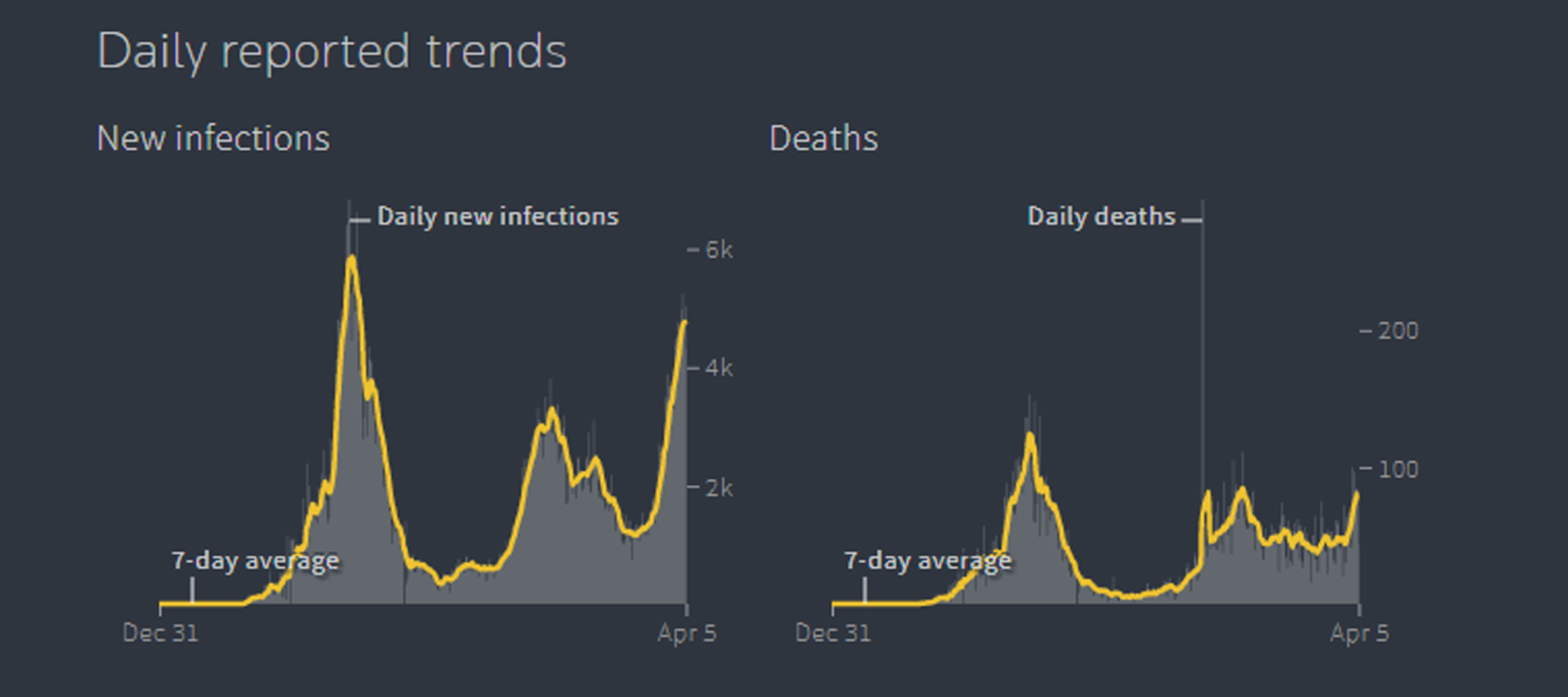
These days, the deaths due to the Covid-19 are at the peak and the rate is still increasing day by day. So, it becomes necessary to predict and forecasts the deaths due to this virus so that to adopt some prevention measures. The first case of Covid-19 was discovered in Pakistan on February 26, 2020, in Karachi, by a man who had recently returned from Iran. Since then, the spread of infections has accelerated, and on March 18, 2020, it was confirmed that the virus had spread to four provinces of Pakistan. Currently, in South Asia, Pakistan is the second highest number of confirmed cases, 19th number of confirmed cases in Asia, and 31st number with the highest confirmed cases in the world. The first death due to Covid-19 was reported in Sindh on 20 March, the third death was confirmed in KPK on 22 March. Since then the number of deaths is increasing and it’s reached the highest figures than some other countries. In the last weeks of June, the cases were decreasing and showing some downward trends. In Fig. 1, the left and right handed graphs show the average increase decrease in the number of infections and deaths respectively.
Fig. 1
Daily New Infections and Deaths of Covid-19.
Many research studies have been conducting on Covid-19, for example, Yousaf et al. [1] studies the forecasting of the infections, deaths, and recoveries using Auto-Regressive Integrated Moving Average Model (ARIMA), Fong et al. [2] discussed the accurate early forecasting model using small data, Petropoulos and Makridakis [3] also discussed the forecasting model, Chen et al. [4] worked on the reconstruction and prediction algorithm for Covid-19, Nayak et al. [5] presented the statistical analysis of Covid-19 using the probabilistic model, Wolkewitz [6] discussed the statistical analysis of the clinical Covid-19 data, Yue et al. [7] worked out the Size of a COVID-19 Epidemic from Surveillance Systems, Syed and Sibgatullah [8] discussed the estimation of the final size of the COVID-19 epidemic in Pakistan using the SIR model, Mizumot et al. [9] estimates the asymptomatic proportion of COVID-19. Many other research studies have been conducted where the investigator applied various statistical tools for data analysis, For example, zeri et al. [10] discussed the comparison of the climate indices using GEE model, Mahmoudi et al. [11] worked on the estimation of the simple harmonizable processes, Maleki and Mahmoudi [12] studied the Two-piece location-scale distribution, Mahmoudi et al. [13] explored the large sample inference in two independent populations, and Pan et al. [14] worked on classifying and comparing several linear and non-linear regression models with a symmetric error.
For modeling and predictions of the lifetime data like Covid-19, there exist, various statistical models to estimate the parameter and predict the pattern of infections and deaths from a particular virus. For example, the Weibull distribution (W) introduced by Wallodi [15], and Exponential distribution (Ex) by Epstein [16] are among others. These models fail to model the data having a non-monotonic hazard rate function. In practice, the data is not all the time following a monotonic failure function, for example, the accidents rate, and the lifetime of a machine to work follow a non-monotonic failure function. To overcome this flaw, researchers are trying to develop new probability models so that to capture a non-monotonic hazard rate function. For example, Cordeiro [17] developed exponential-Weibull distribution (EX-W) while El-Gohary [18] introduced Inverse flexible Weibull extension distribution (EIFW) for capturing flexibility in the data by using the real data of a lifetime of 50 devices and remission times of 128 bladder cancer patients. To overcome the problem of non-monotonicity, Ijaz et al. [19] presented the Gull Alpha Power Weibull distribution (GAPW) has better performances as compared to others existing distributions by using the real data set of bank customers and bladder cancer patients data. For more recent research studies, we refer to see, ijaz et al. [20, 21], and Ali et al. [22].
In this paper, a new model specifically for modeling Covid-19 deaths in Pakistan is designed. In comparison to the existing distributions, the proposed model not only captures a non-monotonic hazard shape but also leads to an adequate fit.
2Material and methodology
In this section, we produced a new family of distributions which is defined as under,
A random variable x is said to be FEF variable if it holds the following cumulative distribution function and Probability density function or in short CDF and PDF respectively
(1)
(2)
For producing new probability models one can choose an appropriate CDF and PDF of the existing functions. In this paper, we have incorporated the CDF and PDF of the Weibull distribution presented by Wallodi Weibull in the above two equations so that to produce a new probability model. The new probability model is then called Flexible Exponential Weibull (FEW) distributions having the following CDF and PDF
(3)
(4)
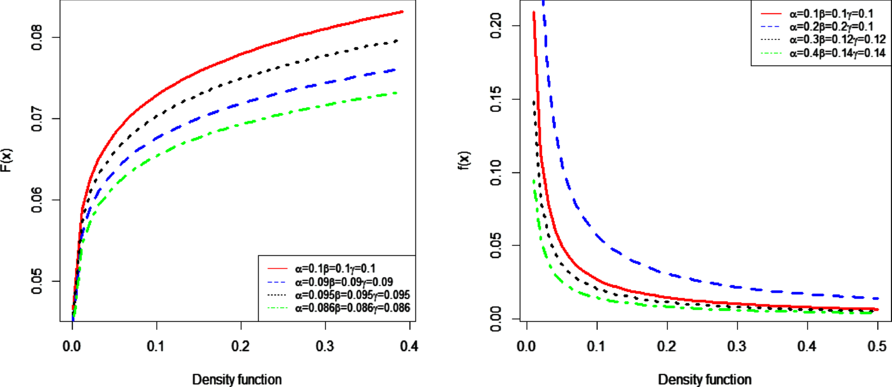
Figure 2 describes various shapes of the CDF and PDF given in Equations (3) and (4) with various parameter values.
Fig. 2
Plots of the CDF and PDF of FEW.
3Other statistical properties
This section describes some important statistical properties of FEW distribution including they are the survival and hazard rate function, Quantile function, moments, order Statistics, Renyi entropy, and Skewness and Kurtosis.
3.1Survival and Hazard rate Function
The survival function can be defined by
(5)
Using the (3) in (5), we get
(6)
(7)
By incorporating the result of Equation (4) and (6) in Equation (7), we obtained
(8)
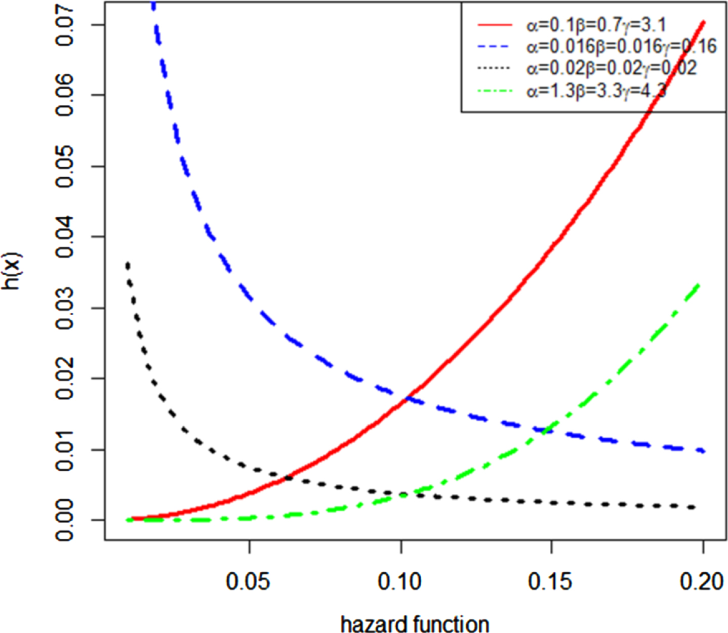
Figure 3 reflects various plots of the hazard rate function by using different values of parameters.
Fig. 3
Plots of the hazard rate function of FEW.
3.2Quantile function
The quantile of FEW can be defined by
(9)
Using Equation (3) and then solve for x, we get
3.3Rth Moments
To study the shape of the distribution, we need to study its four moments. This can be done by finding the Rth moments which is defined by
(10)
By putting Equation (4) in Equation (10), we obtained
The more simplified form of the above expression is
(11)
Using the above supposition in (11), we get the following integral form
(12)
Finally, we obtained the result
(13)
3.4Order statistics
Let X1, X2, X3, ... Xn be ordered random variables from FEW, then the PDF of the ith order statistic is given by
(14)
Using Equation (3) and (4), the smallest and largest order statistics of FEW can be obtained respectively by using i = 1 and i = n as
(15)
(16)
3.5Renyi entropy
The Renyi entropy of the random variable X belong to FEW is defined by
(17)
Recalling Equation (4), we get the following result
The simplified form of the above expression is
(18)
(19)
Finally, we obtained
where
3.6Skewness and Kurtosis
The mathematical expression of the Galton Skewness and Moors kurtosis are as follows
(20)
(21)
Table 1 illustrates the numerical description of the Skewness and Kurtosis for different values of parameters.
Table 1
Numerical values of skewness and Kurtosis
| a | b | c | Skewness | Kurtosis |
| 0.5 | 5.5 | 0.2 | 0.9220822 | 6.372607 |
| 0.5 | 3.5 | 1.2 | 0.1739151 | 1.236659 |
| 0.5 | 5 | 0.4 | 0.6426683 | 2.244966 |
| 0.1 | 7 | 4 | –0.02439357 | 1.217794 |
| 1 | 7 | 4 | –0.04890463 | 1.238134 |
| 10 | 7 | 4 | 0.009419263 | 1.251933 |
| 1 | 10 | 1 | 0.2022893 | 1.260582 |
| 1 | 10 | 0.1 | 0.9949477 | 32.98577 |
| 10 | 10 | 0.1 | 0.8894631 | 6.893794 |
| 10 | 10 | 10 | –0.01252348 | 1.25391 |
3.7Special cases
Then special forms of Equation (3) and (4) can be derived by choosing appropriate values of the parameters. Table 2 presents the special forms of FEW with their corresponding CDF and PDF
Table 2
Special forms of FEW
| Cases | Model | CDF | |
| I. c = 1 | Flexible Exponential Exponential (FEE) |
|
|
| II. c = 2 | Flexible Exponential Rayleigh (FER) |
|
|
3.8Parameter estimation
In this section, the unknown parameters of FEW are estimated by using the maximum likelihood method. The likelihood function of Equation (4) is defined by
(22)
The log likelihood function is given by
(23)
To obtain the parameter values of a, b, and c, we have to take the partial derivatives of Equation (23) with respect to each parameter
(24)
(25)
(26)
Since the above equations are not in closed form but still one can solve these equations numerically by using Mathematical Techniques.
3.9Applications
This section provides the significance of the novel probability model by using the deaths of Covid-19. The data set is taken from Coronavirus Pandemic (Covid-19) statistics and research [23] consisting of daily deaths per million in Pakistan from 02/05/2020 to 04/07/2021. The performance of the proposed model with others is compared by using the Cramer-von mises (W), Anderson darling (A), Akaike information criteria (AIC), Consistent Akaike information criteria (CAIC), Hannan and quin information criteria (HQIC), and Bayesian information criteria (BIC). The mathematical form of these criteria are defined by
It is to be noted that the probability model with the smaller values of these criteria leads to a better fit using this data.
3.10Data set: Covid-19 data for Pakistan (Total deaths in Millions)
The data set values are
0.009, 0.014, 0.014, 0.023, 0.027, 0.032, 0.036, 0.041, 0.05, 0.054, 0.063, 0.095, 0.118, 0.122, 0.154, 0.181, 0.186, 0.213, 0.24, 0.258, 0.276, 0.294, 0.299, 0.389, 0.412, 0.421, 0.435, 0.503, 0.579, 0.611, 0.647, 0.761, 0.797, 0.91, 0.96, 1.073, 1.145, 1.218, 1.272, 1.322, 1.412, 1.553, 1.743, 1.888, 1.992, 2.069, 2.155, 2.327, 2.553, 2.648, 2.712, 2.879, 2.983, 3.196, 3.336, 3.445, 3.486, 3.776, 3.776, 3.952, 4.088, 4.251, 4.459, 4.604, 4.83, 4.984, 5.129, 5.283, 5.419, 5.546, 5.704, 5.962, 6.315, 6.714, 6.985, 7.338, 7.642, 8.013, 8.321, 8.76, 9.063, 9.358, 9.833, 10.209, 10.666, 11.15, 11.15, 11.549, 12.354, 12.852, 13.468, 14.002, 14.618, 15.311, 15.849, 16.252, 16.728, 16.999, 17.669, 17.936, 18.267, 18.643, 18.864, 19.485, 19.897, 20.25, 20.603, 20.603, 20.911, 21.558, 21.907, 22.282, 22.559, 22.898, 23.192, 23.527, 23.84, 24.084, 24.383, 24.564, 24.564, 24.999, 25.207, 25.347, 25.528, 25.7, 25.845, 26.09, 26.198, 26.357, 26.357, 26.447, 26.551, 26.674, 26.818, 26.941, 26.941, 27.054, 27.158, 27.158, 27.226, 27.321, 27.398, 27.47, 27.534, 27.602, 27.67, 27.747, 27.792, 27.855, 27.896, 27.955, 27.955, 28.023, 28.073, 28.109, 28.154, 28.208, 28.267, 28.267, 28.317, 28.371, 28.403, 28.444, 28.448, 28.466, 28.494, 28.512, 28.647, 28.679, 28.702, 28.702, 28.724, 28.747, 28.788, 28.815, 28.838, 28.851, 28.878, 28.896, 28.924, 28.942, 28.969, 29.01, 29.041, 29.046, 29.064, 29.082, 29.118, 29.141, 29.173, 29.204, 29.231, 29.272, 29.308, 29.331, 29.354, 29.422, 29.458, 29.485, 29.485, 29.53, 29.585, 29.625, 29.662, 29.689, 29.743, 29.788, 29.824, 29.883, 29.942, 29.974, 30.051, 30.123, 30.146, 30.209, 30.295, 30.341, 30.399, 30.454, 30.494, 30.508, 30.535, 30.599, 30.671, 30.762, 30.811, 30.888, 30.943, 31.006, 31.088, 31.205, 31.341, 31.432, 31.545, 31.586, 31.69, 31.785, 31.939, 32.106, 32.183, 32.328, 32.414, 32.563, 32.731, 32.812, 34.229, 34.419, 34.687, 34.841, 35.058, 35.325, 35.506, 35.75, 35.954, 36.149, 36.33, 36.629, 36.968, 37.145, 37.394, 37.588, 37.851, 38.019, 38.421, 38.693, 38.947, 39.173, 39.494, 39.82, 39.983, 40.314, 40.789, 41.106, 41.486, 41.876, 42.238, 42.518, 42.89, 43.265, 43.768, 44.153, 44.438, 44.701, 44.95, 45.235, 45.484, 45.746, 46.068, 46.439, 46.679, 46.855, 47.123, 47.358
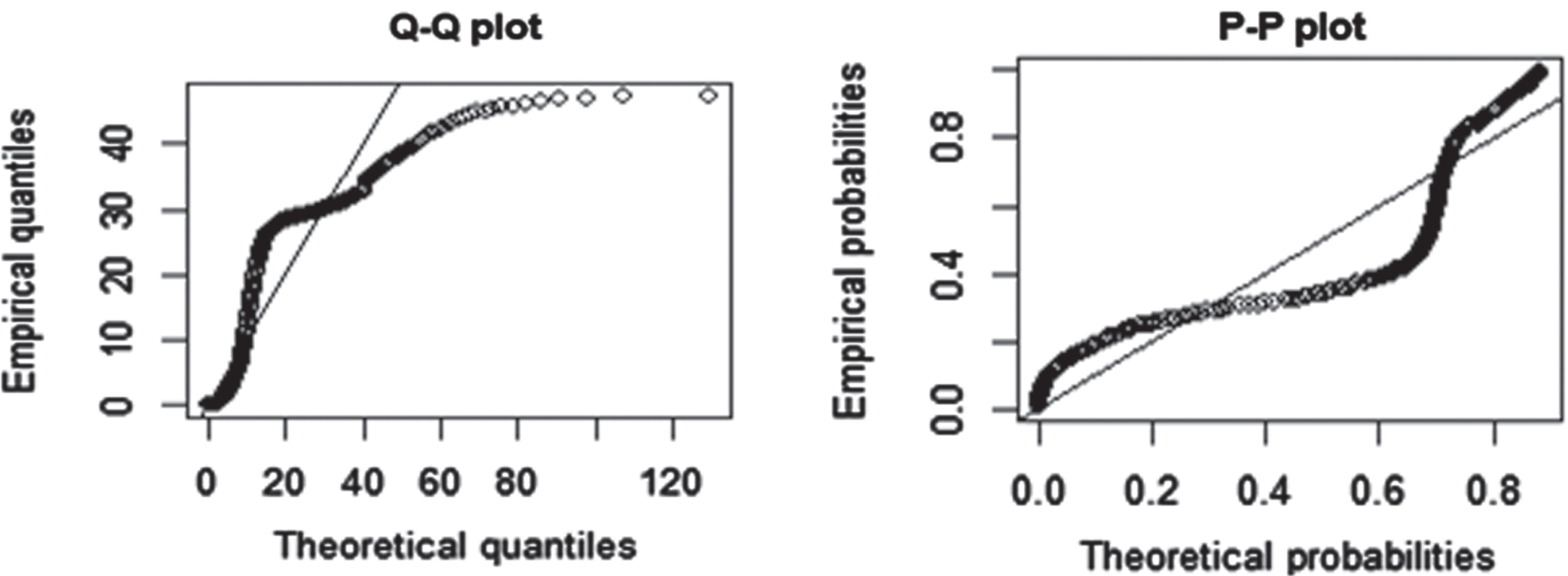
Figure 4 describes the theoretical and empirical PDF, CDF, and TTT plot of the data. The TTT plot clearly defines that this data follows a non-monotonic hazard rate function. Figure 5 defines the Q-Q and P-P plots of FEW.
Fig. 4
Theoretical and empirical PDF and CDF, and TTT plot of FEW.
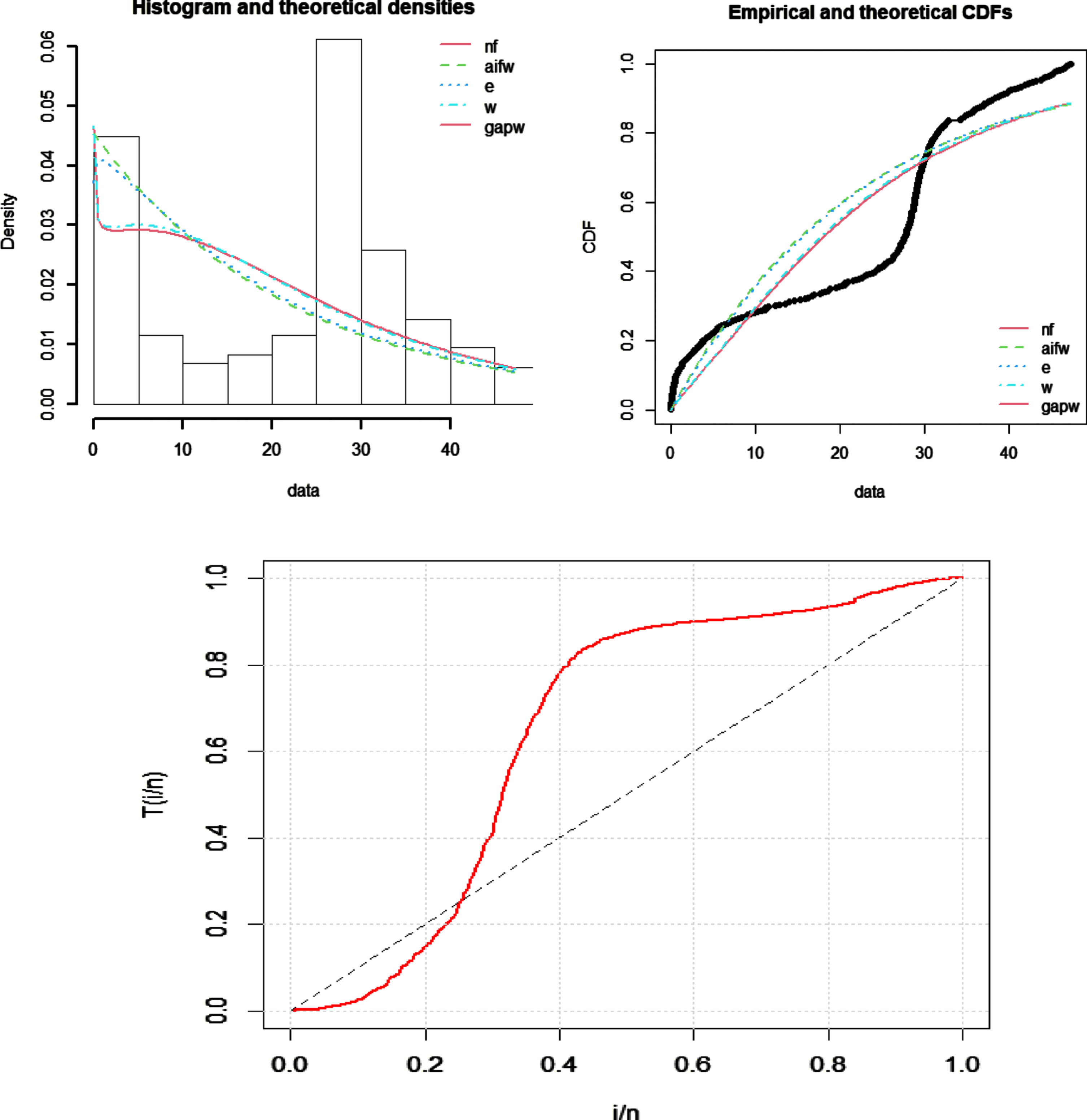
Fig. 5
Q-Q plot and P-P plot of FEW.
The Cramer-von mises (W), Anderson darling (A), maximum likelihood estimates, standard errors, and the log-likelihood values are given in Table 3. Table 4 reflects the values of AIC, CAIC, BIC, and HQIC. The results declared that the smaller values are obtained for FEW among others using these criteria and hence FEW provides a flexible fit over Exponential (E), Weibull (W), Exponential-Weibull (Ex-W), Algoharai Inverse Flexible Weibull (AIFW), and Gull Alpha Power Weibull distribution (GAPW).
Table 3
Maximum likelihood estimates and their standard errors of FEW for Covid-19 data of Pakistan
| Model | W | A | MLE | Standard error | -log likelihood |
| FEW | 4.28435 | 22.26336 | 1.9891214 0.0992052 0.8826092 | 0.35501287 0.02398305 0.06091679 | 1187.638 |
| Ex-W | 4.711372 | 24.59633 | 3.834743 0.999751 –3.796775 | NaN NaN NaN | 1204.855 |
| W | 4.679397 | 24.4247 | 0.04243439 1.02011264 | 0.00814312 0.05432640 | 1203.33 |
| Ex | 4.705066 | 24.56344 | 0.04529655 | 0.00264046 | 1203.454 |
| AIFW | 2.756311 | 13.82258 | 0.01984159 0.05013188 | 0.002082701 0.002646834 | 1229.493 |
| GAPW | 4.339915 | 22.56649 | 0.36241454 0.08512305 0.90828066 | 0.07910969 0.01807806 0.05425457 | 1190.373 |
Table 4
Goodness of fit measures of FEW for Covid-19 data of Pakistan
| Models | AIC | CAIC | BIC | HQIC |
| FEW | 2381.277 | 2381.359 | 2392.327 | 2385.702 |
| Ex-W | 2408.907 | 2408.921 | 2412.591 | 2410.383 |
| W | 2410.659 | 2410.701 | 2418.027 | 2413.61 |
| Ex | 2415.711 | 2415.794 | 2426.762 | 2420.136 |
| AIFW | 2462.986 | 2463.028 | 2470.354 | 2465.937 |
| GAPW | 2386.745 | 2386.828 | 2397.796 | 2391.171 |
3.11Simulations
The simulation study is performed by using the expression given in Equation (9). The experiment is repeated 1000 times with a sample of size n by choosing different values of parameters. The MSE and bias of each parameter are given in Table 5. The result shows that the bias and MSE of each estimator are decreasing when the sample size increases.
Table 5
Bias and Mean Square Errors (MSE)
| Parameters | n | MSE(a) | MSE(b) | MSE(c) | Bias(a) | Bias(b) | Bias(c) |
| a = 2.5 b = 5.05 c = 1.5 | 100 | 8.399835 | 1.674413 | 0.2992278 | 1.299793 | 0.5682359 | 0.3094939 |
| 150 | 8.019119 | 1.574738 | 0.2350304 | 1.297721 | 0.5436203 | 0.2676643 | |
| 200 | 7.20726 | 1.260177 | 0.1953557 | 1.089667 | 0.4537408 | 0.2217462 | |
| 250 | 6.633509 | 1.196652 | 0.1693393 | 1.038047 | 0.4300178 | 0.2060859 | |
| a = 2.4 b = 5.5 c = 1.45 | 100 | 8.451935 | 1.775088 | 0.232134 | 1.126289 | 0.5177107 | 0.2444374 |
| 150 | 6.575859 | 1.425732 | 0.1829624 | 0.9139166 | 0.3883343 | 0.2006606 | |
| 200 | 5.671356 | 1.112708 | 0.1598493 | 0.8035166 | 0.3496737 | 0.1794062 | |
| 250 | 4.711099 | 0.912254 | 0.1439866 | 0.7322363 | 0.32681 | 0.165537 |
4Conclusion and Discussion
This paper proposes a novel probability model for modeling the Covid-19 data. The proposed model is called FEW, various statistical properties are derived including the estimation of parameters. In order to evaluate the significance of the parameter estimates, a simulation study is conducted. Moreover, the proposed model is compared with already existing probability models by using the death data of Covid-19 in Pakistan. It has been observed that the novel probability model is a better choice and is supposed to increase the model flexibility regarding Covid-19 data. Hence, the proposed probability distribution can be used to predict efficiently the pattern of deaths due to Covid-19 or some other pandemic like the Dengue virus, etc. In order to minimize the rate of mortality, this model will help the health practitioners to determine the estimated figures with certain preventive measures.
References
[1] | Yousaf M. , Zahir S. , Riaz M. , Hussain S.M. and Shah K. , Statistical analysis of forecasting COVID-19 for upcoming month in Pakistan, Chaos, Solitons & Fractals 138: ((2020) ), 109926. |
[2] | Fong S.J. , Li G. , Dey N. , Crespo R.G. and Herrera-Viedma E. , Finding an accurate early forecasting model from small dataset: A case of -ncov novel coronavirus outbreak, ((2020) ). arXiv preprint arXiv:2003.10776. |
[3] | Petropoulos F. and Makridakis S. , Forecasting the novel coronavirus COVID-19, PloS one 15: (3) ((2020) ), e0231236. |
[4] | Chen Y. , Cheng J. , Jiang X. and Xu X. , The reconstruction and prediction algorithm of the fractional TDD for the local outbreak of COVID-19, ((2020) ). arXiv preprint arXiv:2002.10302. |
[5] | Nayak S.R. , Arora V. , Sinha U. and Poonia R.C. , A statistical analysis of COVID-19 using Gaussian and probabilistic model, Journal of Interdisciplinary Mathematics ((2020) ), 1–14. |
[6] | Wolkewitz M. , Lambert J. , von Cube M. , BugieraL., GroddM., HazardD.,... KaierK., Statistical analysis of clinical covid-19 data: A concise overview of lessons learned, common errors and how to avoid them, Clinical Epidemiology 12: ((2020) ), 925. |
[7] | Yue M. , Clapham H.E. and Cook A.R. , Estimating the size of a COVID-19 epidemic from surveillance systems, Epidemiology (Cambridge, Mass.) 31: (4) ((2020) ), 567. |
[8] | Syed F. , Sibgatullah S. , (2020). Estimation of the final size of the COVID-19 epidemic in Pakistan. MedRxiv. |
[9] | Mizumoto K. , Kagaya K. , Zarebski A. and Chowell G. , Estimating the asymptomatic proportion of coronavirus disease (COVID-19) cases on board the Diamond Princess cruise ship, Yokohama, Japan, 2020, Eurosurveillance 25: (10) ((2020) ), 2000180. |
[10] | Zarei A.R. , Shabani A. and Mahmoudi M.R. , Comparison of the climate indices based on the relationship between yield loss of rain-fed winter wheat and changes of climate indices using GEE model, Science of The Total Environment 661: ((2019) ), 711–722. |
[11] | Mahmoudi M.R. , Nematollahi A.R. and Soltani A.R. , On the detection and estimation of the simple harmonizable processes, Iranian Journal of Science and Technology (Sciences) 39: (2) ((2015) ), 239–242. |
[12] | Maleki M. and Mahmoudi M.R. , Two-piece location-scale distributions based on scale mixtures of normal family, Communications in Statistics-Theory and Methods 46: (24) ((2017) ), 12356–12369. |
[13] | Mahmoudi M.R. , Behboodian J. and Maleki M. , Large sample inference about the ratio of means in two independent populations, Journal of Statistical Theory and Applications 16: (3) ((2017) ), 366–374. |
[14] | Pan J.J. , Mahmoudi M.R. , Baleanu D. and Maleki M. , On comparing and classifying several independent linear and non-linear regression models with symmetric errors, Symmetry 11: (6) ((2019) ), 820. |
[15] | Weibull W. , Wide applicability, Journal of Applied Mechanics 103: (730) ((1951) ), 293–297. |
[16] | Epstein B. , (1958). The exponential distribution and its role in life testing. WAYNE STATE UNIV DETROIT MI. |
[17] | Cordeiro G.M. , Ortega E.M. and Lemonte A.J. , The exponential–Weibull lifetime distribution, Journal of Statistical Computation and Simulation 84: (12) ((2014) ), 2592–2606. |
[18] | El-Gohary A. , El-Bassiouny A.H. and El-Morshedy M. , Inverse flexible Weibull extension distribution, International Journal of Computer Applications 115: (2) ((2015) ), 46–51. |
[19] | Ijaz M. , Asim S.M. , Farooq M. , Khan S.A. and Manzoor S. , A Gull Alpha Power Weibull distribution with applications to real and simulated data, PloS one 15: (6) ((2020) ), e0233080. |
[20] | Ijaz M. , Asim M. , Khalil A. , (2019). Flexible Lomax distribution. |
[21] | Ijaz M. , Mashwani W.K. and Belhaouari S.B. , A novel family of lifetime distribution with applications to real and simulated data, Plos one 15: (10) ((2020) ), e0238746. |
[22] | Ali M. , Khalil A. , Ijaz M. and Saeed N. , Alpha-Power Exponentiated Inverse Rayleigh distribution and its applications to real and simulated data, PloS one 16: (1) ((2021) ), e0245253. |
[23] | https://github.com/owid/covid-19-data/raw/master/public/data/owid-covid-data.xlsx |

