A fully automated Dobson sun spectrophotometer for total column ozone and Umkehr measurements

Stübi, René; Schill, Herbert; Klausen, Jörg; Maillard Barras, Eliane; Haefele, Alexander

doi:https://doi.org/10.5194/amt-14-5757-2021

Articles | Volume 14, issue 8

https://doi.org/10.5194/amt-14-5757-2021

Articles | Volume 14, issue 8

Research article

23 Aug 2021

Research article |

| 23 Aug 2021

A fully automated Dobson sun spectrophotometer for total column ozone and Umkehr measurements

René Stübi, Herbert Schill, Jörg Klausen, Eliane Maillard Barras, and Alexander Haefele

Abstract

The longest ozone column measurement series are based on the Dobson sun spectrophotometers developed in the 1920s by Prof. G. B. W. Dobson. These ingenious and robustly designed instruments still constitute an important part of the global network presently. However, the Dobson sun spectrophotometer requires manual operation, which has led to the discontinuation of its use at many stations, thus disrupting long-term records of observation. To overcome this problem, MeteoSwiss developed a fully automated version of the Dobson spectrophotometer. The description of the data acquisition and automated control of the instrument is presented here with some technical details. The results of different tests performed regularly to assess the instrument's good working conditions are illustrated and discussed.

Compared to manual operation, automation results in a higher number of daily measurements with lower random error and additional housekeeping information to characterize the measuring conditions. The automated Dobson instrument allows for continuous observation of the ozone column with a resolution of ∼ 1 DU under clear-sky conditions.

Download & links

Article (PDF, 2193 KB)

How to cite

How to cite.

Dates

Received: 28 Sep 2020 – Discussion started: 10 Dec 2020 – Revised: 07 May 2021 – Accepted: 21 May 2021 – Published: 23 Aug 2021

1 Introduction

Solar UV radiation is generally split into three ranges called UVC (100 nm $\leq λ < 280$ nm), UVB (280 nm $\leq λ < 315$ nm) and UVA (315 nm $\leq λ < 400$ nm). At ground level, harmful UVC radiation is completely blocked by the ozone layer while in the intermediate UVB–UVA range (300 nm $< λ < 330$ nm) is predominantly controlled by it. Most ozone-monitoring instruments are based on the measurement of the absorption of this part of the solar spectrum. The detection of the ozone layer depletion is one of the most important scientific achievements of the 20th century and had a significant impact on raising awareness of man's influence on the Earth's climate (Solomon, 2019). Following its discovery and the implementation of the Montreal Protocol, the signatory states committed themselves to continued monitoring of the state of the ozone layer. Model simulations predict a recovery of the ozone layer that will last for several decades rather than years depending on the location on the Earth and on the altitude considered (SPARC/IO3C/GAW, 2019; WMO, 2018). Moreover, the uncertainties associated with the climate change feedback on the ozone recovery process require very precise measurements and long-term stability of instruments.

Today, the main sources of information come from the global survey with multiple instruments on board satellites. However, the long development period to prepare a satellite mission, its relatively short lifetime and the risk of failure or of calibration drifts call for reference ground-based measurements for sustained monitoring. Following the 1957–1958 International Geophysical Year, the network of Dobson instruments was established with additional stations worldwide under the lead of the NOAA in Boulder (Dobson, 1968). Similarly, after the development of the commercially available Brewer sun spectrophotometer, the network of Brewer instruments grew with the support of the Canadian group in Toronto (Kerr et al., 1981; Fioletov et al., 2005). Presently, both Dobson and Brewer reference networks are operated in parallel to monitor long-term changes of the ozone column.

The principle of the instrument developed by Dobson in the early 1920s is based on measurements of the intensity of ozone-attenuated radiation in a number of narrow spectral bands. This was first done by analysing spectra recorded on photographic plates; later the radiation intensity was measured with photoelectric detectors within the instrument and nowadays with photomultiplier tube (PM) detectors. Many of the Dobson instruments manufactured in the 20th century are still used operationally and, together with Brewer instruments, constitute the backbone of the global ozone column monitoring network (Komyhr, 1980; Komhyr et al., 1989).

Measurements from the Dobson and Brewer networks produce reference ozone column measurements to which satellite instruments, models and other types of ground-based instruments can be compared. These intercomparisons make it possible to detect problems with any one of the measurement systems or networks. The processing algorithm of the Dobson and Brewer data is still subject to further analyses and improvements as documented in the scientific literature. These mainly concern updates of the underlying ozone cross-sections, stray light bias corrections or the calibration process to ensure network homogeneity (Redondas et al., 2014; Moeini et al., 2019; Christodoulakis et al., 2015).

At Arosa, Dobson instruments have been operated since 1926, resulting in the longest continuous time series worldwide. Historically, the Arosa Licht-Klimatisches Observatorium (LKO) development was strongly linked to the Dobson instrument network extension promoted by Dobson in the first half of the 20th century (Staehelin and Viatte, 2019; Brönnimann et al., 2003; Perl and Dütsch, 1958; Scarnato et al., 2010; Staehelin et al., 2018). In the early 1920s, the ozone column measurements revealed a seasonal variability at mid-latitude linked to the stratospheric circulation. In the 1950s, these ozone variations were studied further, and it was shown that they were related to the synoptic weather patterns and could be used to improve the weather forecasts (Breiland, 1964). While the usefulness of LKO measurements has been regularly questioned over the course of the 20th century, with the discovery of ozone layer depletion by CFCs, the measurement programme continued as part of the global effort to verify that the Montreal Protocol was working (Albrecht and Parker, 2019; Solomon, 1999). A first Brewer instrument (B₀₄₀, MKII) was acquired in 1988 to expand the fleet of instruments and possibly make a transition to a partly or fully automated ozone monitoring station. Two additional Brewer instruments were subsequently purchased in 1991 (B₀₇₂, MKII) and 1998 (B₁₅₆, MKIII) and operated in parallel with the Dobson instruments D₁₀₁ and D₀₆₂ (Stübi et al., 2017 a). For 15 years, the Dobson and Brewer instrument triads were operated in parallel in Arosa. More recently, all instruments were relocated to nearby Davos. This relocation, in combination with the automation of the Dobson operation, allows for continuation and improvement of this observation programme, with reduced operational cost.

The present publication describes the successful MeteoSwiss developments of an automated version of the Dobson sun spectrophotometer. Today, the three instruments from LKO are fully automated for the ozone column measurements in the direct sun mode as well as observations in the Umkehr mode. The lamp tests remain semi-automated, and an operator still has to set the lamps in place before launching the automated recording of the tests.

This paper is published in parallel with the analysis of the LKO Dobson instrument data using the manual and automated modes side by side (Stübi et al., 2021). Therefore, only few measurement results will be presented here, and the reader is invited to look at this separate publication for more information. Similar studies with LKO Brewer instruments have also been published recently (Stübi et al., 2017 a, b).

The paper is organized as follows: in Sect. 2, the Dobson instrument measurement principles are described. In the different subsections of Sect. 3, the details of the transition from manual to automated measurements are presented. Discussion and conclusion follow in Sect. 4 and 5.

2 Dobson measurement principle and instrument design

The principle of the Dobson instrument, its operation and its data handling are described in many publications (Komyhr, 1980; Evans, 2008; Basher, 1982). An illustration of the essential parts of a Dobson instrument can be seen in Fig. 1 of Evans et al. (2017). The measurement principle is based on the comparison of the solar irradiance in two narrow bands of the UV radiation spectrum selected by a pair of slits: the narrower slit selects the short wavelength window, λ_s, largely attenuated by the ozone in the atmosphere, while the wider slit selects the long wavelength window, λ_l, mostly unaffected by ozone. The detection is based on the comparison of the intensities along each optical path as the slits are opened and closed by a rotating wheel. Since the absolute measurement of weak signals was quite challenging at the time of the development of the instrument, Dobson introduced a calibrated attenuator in front of the long wavelength slit to attenuate the intensity of λ_l to the level of the λ_s intensity. The attenuator thus imprints the effect of ozone at λ_s along the light path in the atmosphere at the non-absorbing wavelength λ_l. The measurements consist in adjusting the attenuator in order to get a differential signal from the two slits of zero. For the Dobson instrument, the three commonly used wavelength pairs are referred to as A, C and D, while their combinations are referred to as the double pairs AC, AD and CD. The Dobson instrument is a double monochromator with a dispersing prism in front of the slits and a second prism after the slits to redirect the optical paths onto the PM detector. The optical attenuator consists of a moving neutral-density filter (the optical “wedge”) attached to a graduated rotating disc (R dial). As the slits are fixed to the frame of the instrument, the wavelength pair selection is achieved by rotating a pair of a quartz plates (Q1 lever, Q2 lever) through which the light beam passes.

The ozone column density is related to the measured irradiance intensity at the surface according to the Beer–Lambert law (Shaw, 1983; Moeini et al., 2019):

\begin{matrix} (1) & I (λ) = I_{0} (λ) \cdot e^{- τ (λ)} \end{matrix}

with

τ (λ) = α (λ) \cdot X \cdot μ + β (λ) \cdot \frac{p}{p_{0}} \cdot m_{R} + δ (λ) \cdot m_{M},

where I₀(λ) is the extraterrestrial irradiance, and the optical thickness τ(λ) of the incident path is the sum of the ozone absorption, the Rayleigh and the Mie scattering terms. The coefficients α(λ) and β(λ) are calculated based on the nominal values of the optical characteristics of the primary reference instrument (Komhyr et al., 1989). The strict similarity of the mounting of the optical elements (e.g. slits, mirrors, lenses) in all Dobson instruments justifies these common α and β values. From the calibration response of the attenuator, the R-dial reading is converted to the relative intensity N(λ_s,λ_l) for a pair of wavelengths as $N = \log (\frac{I_{s 0}}{I_{l 0}}) - \log (\frac{I_{s}}{I_{l}})$ . Subsequently, the double pairs are formed to eliminate the small contribution of the Mie scattering since it is almost constant in the λ_s–λ_l range:

\begin{matrix} (2) & \begin{aligned} O_{3} & = X_{AD} \\ = \frac{\begin{matrix} (N_{A} - N_{D}) - [{(β^{s} - β^{l})}_{A} - {(β^{s} - β^{l})}_{D}] \frac{m p}{p_{0}} \\ - [{(δ^{s} - δ^{l})}_{A} - {(δ^{s} - δ^{l})}_{D}] \sec (SZA) \end{matrix}}{[{(α^{s} - α^{l})}_{A} - {(α^{s} - α^{l})}_{D}] μ}, \end{aligned} \end{matrix}

where the ratio $p / p_{0}$ is a correction of the Rayleigh term for the mean pressure p at the station.

Table 1Dobson instruments nominal values of λ_s (nm) and λ_l (nm) centre lines and FWHM, as well as the equivalent values for the LKO Dobson instruments. The FWHM values of D₀₆₂ and D₀₅₁ are similar to those of D₁₀₁, so they are not reported in this table.

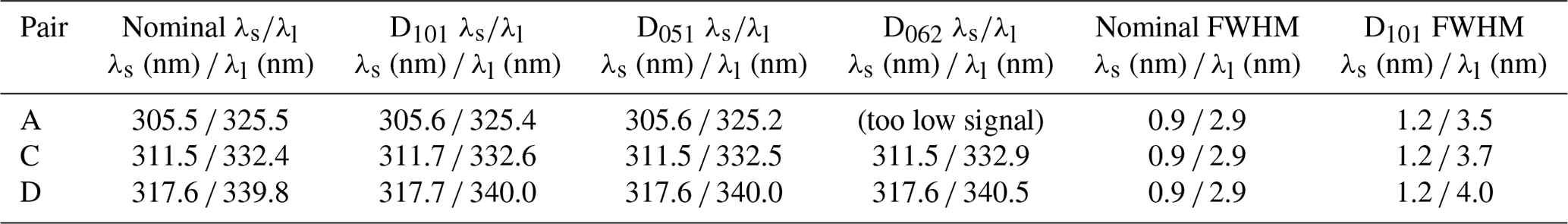
Download Print Version | Download XLSX

Table 1 gives the nominal optical characteristics of the primary reference Dobson instrument, as well as those of the LKO instruments (Komhyr et al., 1989). The slits from D₁₀₁ were measured at the Physikalisch-Technische Bundesanstalt using a spectrally tuneable laser (Köhler et al., 2018), while slits from D₀₆₂ were characterized at LKO using the tuneable and portable radiation source (TuPS) instrument (Šmíd et al., 2021). Even though the nominal and the actual values of the slit centre wavelengths agree well, significant differences exist for the full width at half maximum (FWHM) values. Similar differences have been reported in Köhler et al. (2018) for different Dobson instruments characterized during the ATMOZ project (Gröbner et al., 2017). The authors have quantified the effects of these differences on the calculated ozone column and conclude that for the commonly used double pair AD, the ozone values could be biased up to ∼ 1 % depending on the instrument. Future advanced data reprocessing will incorporate these recent slit measurements for accurate comparison between different types of instruments.

In addition to the total ozone column measurements possible with Dobson instruments, the Umkehr method permits low-resolution ozone profiles to be retrieved from the measurements of relative intensities N(λ_s,λ_l) of zenith observations during early morning and late afternoon hours. As the solar zenith angle (60^∘ < SZA < 90^∘) is increasing, the two intensities λ_s and λ_l decrease, λ_s more rapidly than λ_l. When the effective scattering height for the shorter wavelength λ_s is above the ozone layer, its intensity decreases less rapidly because the absorption occurs mostly after the scattering event. The N(λ_s,λ_l) measurements present a maximum as illustrated in Fig. 4 before 06:00 UTC. This curve bending is called the Umkehr effect (Mateer, 1964). The ozone profiles from the ground up to 50 km are retrieved with a vertical resolution of 5–10 km from the N(λ_s,λ_l) curves by an optimal estimation method (Petropavlovskikh et al., 2005).

3 Automation of the LKO Dobson instruments

The instrument and observation facilities have benefited from numerous improvements over the years. A major change occurred in 1988 with the introduction of a rotating cabin illustrated in Fig. 1a that greatly simplified the manual operation of the Dobson instruments (Hoegger et al., 1992; Staehelin et al., 1998). Previously, instruments were moved out of their shelter on a trolley, and then measurements were initiated. The rotating cabin had an opening in the roof and a turntable with two opposing Dobson instruments that could be rotated to face the sun within seconds. The new setup allowed the number of measurements to be increased and the data quality and reproducibility to be improved since the following conditions were true:

Within 3 min, the C–D–A measurements sequence could be performed with two instruments.
Digital recording of the time, the R-dial position and the instrument temperature was introduced.
The cabin had a controlled temperature so that the instruments were no longer exposed to large diurnal temperature changes.
The “ready-to-measure” status permitted us to take measurements during short sunny periods in changing weather conditions.

https://amt.copernicus.org/articles/14/5757/2021/amt-14-5757-2021-f01

Figure 1Illustration of the transition from manual to automated Dobson measurements. (a) Operator in the rotating cabin with two Dobson instruments on a turntable and with an open skylight in the roof. (b) Two automated Dobson instruments each on its rotating table.

Download

The first attempts at a Dobson automation were made in the 1970s to reduce the effort for the Umkehr measurements that are required to start in the morning before sunrise until the solar zenith angle reaches SZA = 60^∘ and to restart the measurements in the evening from SZA = 60^∘ till after sunset. Räber (1973) describes this first LKO realization of a Dobson automation. While it was successful for the Umkehr measurements for a fixed wavelength pair (e.g. C pair), the results were not conclusive for direct sun ozone column observations due to difficulties with the active sun pointing mechanism, as well as with the wavelength settings (Q-lever positioning). In 2010, the decision was made at MeteoSwiss to develop a fully automated version of the Dobson instrument. The conditions were to leave the internal optical parts of the instruments untouched to avoid any change in the measurement principle and to still allow for manual operation if necessary. The result of this effort is illustrated in Fig. 1.

Figure 1b shows the interior of the container with two automated Dobson instruments sitting side by side on lifting tables. The Dobson instrument, the data acquisition system and the computer are all placed on a large aluminium plate that is mounted on a turntable, which follows the sun azimuth. The solar radiation enters the instrument via the sun-director prism that protrudes from the roof of the container and is protected from adverse weather conditions by a quartz dome. The dome is made of high-quality UV fused silica with an internal diameter of 12 cm. Tests with and without the dome above the sun director proved that it does not affect the measured radiation intensities' ratios.

Dobson instruments D₀₅₁ and D₀₆₂ were automated between the inter-comparisons 2010 and 2012. Dobson instrument D₁₀₁ was manually operated until early 2014. The extended 2012–2014 development period allowed us to compare the manual and automated measurements (Stübi et al., 2021).

3.1 Instrument control

The Dobson standard operating procedure of the WMO recommends measuring the ozone column at selected SZA values to cover the air mass range $1 < μ < 5.8$ (Evans, 2008). This yields around 20 measurements in summer clear-sky days but only a few measurements in winter. The automation of the LKO Dobson instruments allows us to record the regular sequence of the three wavelength pairs C, D and A during the whole day from sunrise to sunset. With the operational parameters, a C–D–A measurement sequence takes typically 150 s. At the alpine Arosa site, the sun is above the local horizon for 4.5 h in winter, representing ∼ 100 measurements for a sunny day, while in summer up to 250 measurements are recorded.

The Dobson instrument measurements require the control of five rotational axes:

The sun’s image must fall on the entrance window of the instrument; thus the sun’s azimuth and elevation must be tracked. This require two rotation axes.
The synchronous rotation of the two quartz plates to select the appropriate wavelengths pair C, D or A and to compensate effects of the instrument temperature involves two more synchronized rotational axes.
The R-dial rotating disc that drives the calibrated optical attenuator wedges is the fifth axis.

The calculated azimuth of the sun is followed by the rotating table (http://www.dr-clauss.de, last access: 22 July 2021; RODEON JumboDrive), which is driven by a stepping motor and controlled by a differential encoder with a resolution of 0.05^∘. Similarly, the sun elevation is followed using an absolute encoder–motor small assembly (http://en.robotis.com, last access: 22 July 2021; DYNAMIXEL) directly mounted on the sun director support. This device controls the prism orientation with a belt. The three other axes are driven by brushless DC motors and encoders co-axially mounted on the Q1 and Q2 levers and on the R dial. The data acquisition and control system are based on commercially available National Instrument (NI) components and the NI LabView programming language (http://www.ni.com, last access: 22 July 2021; PXI, LabVIEW). The interface between the NI motion control device (part NI-7340) and the motors (http://www.maxongroup.ch, last access: 22 July 2021; EC motor) and encoders (http://www.baumer.com, last access: 22 July 2021; BHG incremental encoder) is realized with a commercially available controller box (http://www.sci-consulting.ch, last access: 22 July 2021; SCmotion, mcDLA).

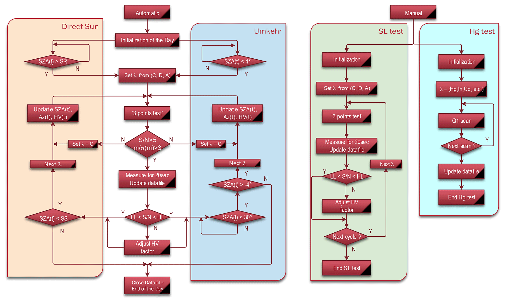
https://amt.copernicus.org/articles/14/5757/2021/amt-14-5757-2021-f02

Figure 2Schema of the data acquisition program's main steps for direct sun, Umkehr, standard lamp and Hg lamp measurements.

Download

The controlling software was developed by Sci-Consulting Ltd. (http://www.sci-consulting.ch) in close cooperation with MeteoSwiss. The software architecture consists of micro-sequences that are called by a sequencer defining the chain of operations to fulfil the dedicated tasks. Figure 2 displays a chart of the major sequences of the data acquisition program: the left side refers to the automated operation for the direct sun and the Umkehr measurements. The right side refers to the semi-automated standard lamp and Hg lamp tests. Following the initialization of the daily files and referencing of the encoders, the system waits for the calculated time of the sunrise at the station. After setting the Q levers for the first wavelength pair and reading the initial R-dial position R_init and the PM high voltage (HV) from the configuration file, the system adjusts these initial values to the actual conditions with the “three-point test”. This latter consists of measuring the PM signal dlaP (digital lock-in amplifier in phase with the selector wheel) (5 s average) for three successive R-dial positions defined as

\begin{matrix} (3) & \begin{aligned} R_{1} = R_{init}, R_{2} = R_{1} \cdot (1 + sign ({dlaP}_{1}) \cdot 0.05), \\ R_{3} = R_{2} \cdot (1 + sign ({dlaP}_{2}) \cdot 0.05) . \end{aligned} \end{matrix}

From the three pairs of points (R_i, dlaP_i), the R value corresponding to dlaP ≈ 0 is inter- or extrapolated depending on sign (dlaP). The three-point test determines the sensitivity of the PM response $δ (dlaP) / δ (R)$ as a Dobson operator would do with small back and forth R-dial rotations to adjust the HV. The data acquisition program similarly adapts the HV (within preset high/low limits) or repeats the three-point test until the PM response is above a predefined threshold. Figure 3a shows a few three-point test results: the R-dial positions follow the yellow line (left scale) and the PM dlaP response the corresponding blue line (right scale). The test results are recorded as housekeeping information for quality control purposes. Once the R value for the dlaP ≈ 0 condition is found, a proportional–integral–derivative (PID) controller acts on the R-dial position to maintain the PM signal close to zero for an averaging period of 20 s. Then the loop restarts with the next wavelength until completion of a C–D–A cycle. All the parameters controlling the timing or threshold conditions of the measurement procedure are stored in a configuration file and can be adapted to local conditions. This setup ensures a large flexibility of the data acquisition and instrument control program.

https://amt.copernicus.org/articles/14/5757/2021/amt-14-5757-2021-f03

Figure 3Screen capture of the real-time data acquisition system since this information is not recorded. (a) Time series of the R dial (yellow line) and the digital look-in amplifier signal dlaP (blue line) with the distinct three-point tests. The green line is from a luxmeter instrument pointing to the zenith. (b) FFT of the dlaP signal with the chopper frequency (∼ 29 Hz) is marked by the vertical blue line and the average noise (∼ 10⁻⁴) between 10 and 200 Hz by the horizontal blue line. The yellow lines are the FFT of the background noise measured on a short circuit.

Download

Umkehr measurements follow the same sequences as direct sun measurements except that the Dobson instrument points to the zenith, and sun elevation routine is skipped. Umkehr data acquisition parameters are adapted to the lower light intensity and the different start/end of measurement conditions, etc.

The standard lamp test procedure illustrated in the right part of Fig. 2 is also similar to direct sun observations, except that the sun pointing routines are skipped. For the Hg lamp test, the Q1 lever is moved at a predefined interval to scan the Hg spectral line at 312.96 nm. The PM dlaP values are averaged for 5 s at successive Q1 positions. Examples of the results of these two tests are illustrated in Fig. 6 and presented in Sect. 3.4. The operator has to set the lamp in place and let the program record a dozen C–D–A cycles with a standard lamp or a dozen scans of a Hg lamp line, for stable and reproducible results.

3.2 Photomultiplier tube signal treatment

The signal amplifier board for the PM signal modulated by the selector wheel rotation was updated to use recent electronic components. It has been designed for a current amplifier (OPA129U) directly connected to the PM output. There is a low pass filter with a cutoff frequency of ∼ 300 Hz to mitigate the Nyquist folding. The data acquisition system records the selector wheel position indicated by a photodiode, and the amplified PM output AC signal is analysed with a digital look-in amplifier (dla), essentially by extracting the Fourier series coefficient at the frequency of the selector wheel.

A dynamical control of the system is achieved via a fast Fourier transform (FFT) analysis (frequency, signal-to-noise) to adapt the data acquisition parameters continuously. Figure 3b shows an example of the FFT of the dlaP (pink line), where the vertical line indicates the measured selector wheel frequency. The horizontal line indicates the median noise level calculated in the frequency range 10–200 Hz. This is mainly generated by the PM HV, and it is 2–3 orders of magnitude higher than the data acquisition noise level (yellow line). The FFT is calculated on blocks of data (sampling rate 60 kHz), whose size corresponds to a multiple of the selector wheel period to improve the noise rejection. The system feedback loop acts on the R-dial motor to maintain the PM signal as low as possible.

The PM high voltage values for a few SZA values are defined in the configuration file and linearly interpolated in between. It is adapted to the actual measuring conditions using the noise level measurements: if the noise falls below a lower limit, the HV is increased by 5 %, and if the noise exceeds an upper limit, the HV is decreased by 5 %. The adaptation factor is limited to ±10 % of normal value. With these controlled noise level conditions, the three-point test gives a measure of the PM signal sensitivity with the ratio $δ (dlaP) / δ (R)$ . Accurate measurements can only be realized if the signal-to-noise ratio is ≥ 1. This parameter can thus be used to control the measurements in real time and/or for the offline quality control of the data.

Fast changing solar irradiance associated with clouds is difficult to deal with. Bright sun can suddenly be completely blocked by a thick cloud, decreasing the PM signal by several orders of magnitude. Too fast an increase of the PM high voltage would result in a saturated PM when the sun reappears. To avoid an oscillation of the R-dial feedback, the acquisition parameters had to be determined empirically. For example, the 5 % step change of the HV values limited to ±10 % has been found to be adequate for scattered cloud conditions.

3.3 Measurements results

Figure 4 illustrates the results of the automated Dobson instrument D₀₅₁ measurements for the sunny day of 7 July 2020. The R-dial positions for three wavelengths pairs C, D and A are shown in panel (a), starting with the Umkehr measurements until 06:00 UTC and direct sun observations for the rest of the day. The corresponding ozone columns for the double pairs AD, AC and CD are shown in panel (b). The reference AD ozone column showed low point-to-point differences of ≤ 1 DU and a smooth variation during the day. The AC double pair showed a systematic low bias of ∼ 2 DU compared to the AD double pair and twice larger point-to-point fluctuations. The CD double-pair ozone column was 2 % higher than the AD and had a scatter of ∼ 2 %. The standard deviations of the R dial for 20 s averages were ≤ 0.2^∘ in such sunny conditions and were therefore smaller than the symbols used in the figure.

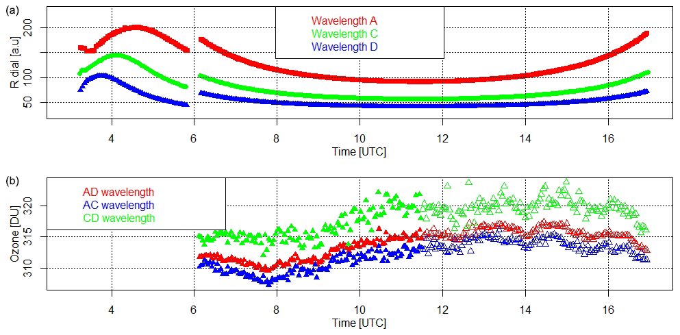
https://amt.copernicus.org/articles/14/5757/2021/amt-14-5757-2021-f04

Figure 4Time series of the measurements for 7 July 2020 with Dobson instrument D₀₅₁. (a) Time series of the R-dial positions. (b) Corresponding ozone column values for the double pairs AD, AC and CD. Filled symbols correspond to the morning and open symbols to the afternoon time period with respect to local noon. The standard deviations of the R dial for 20 s averages are smaller than the symbols used.

Download

https://amt.copernicus.org/articles/14/5757/2021/amt-14-5757-2021-f05

Figure 5Time series of the housekeeping parameters corresponding to the measurements of Fig. 4a with the same colour coding. (a) Time series of the median value of the FFT transform integrated between 10 and 200 Hz. The horizontal black lines correspond to the high and low limit controlling the HV corrections. (b) Time series of the signal-to-noise ratio $S / N = | (δ (dlaP) / δ (R)) | / median (\int FFT (λ) d λ)$ .

Download

The Umkehr data are also very smooth and show the wavelength-dependent Umkehr points clearly where the various R-dial curves exhibit their maxima. The switchover from Umkehr to direct sun observation for Dobson instrument D₀₅₁ was done manually since the option to remove the sun director device has not been automated.

Figure 5 illustrates the housekeeping information measured in parallel to the measurements of Fig. 4. The noise level deduced from the FFT analysis of the measurements in panel (a) shows high values due to the high voltage of the PM necessary to measure the very low intensity of the zenith scattered light at sunrise. Correspondingly, in panel (b), the signal-to-noise ratios are close to 1 initially and gradually increase afterwards. After 06:00 UTC, the direct sun measurements present better signal-to-noise ratios. A transition happened at 11:00 UTC, when the noise level of the A-wavelength pair dropped below the lower limit (lower black line), and the HV of the PM was increased by 5 % of the prescribed values. It stayed the same for the rest of the day.

3.4 Automation of instrument tests

Once the measurement procedure had been developed, the data acquisition (DAQ) system could be evolved to perform other specific tasks. The more common ones are the standard lamp and Hg lamp tests performed weekly to ensure the stability of operation of the Dobson instruments. As illustrated in Fig. 2, the standard lamp test procedure is similar to the direct sun measurements with no assessment of the sun position and different settings for the HV and R_init values. Figure 6a shows the results of standard lamp tests successively using three different standard lamps. The C and D wavelength pair R-dial values were very stable to within ≤ 0.05^∘, while the A pair results varied within ≤ 0.1^∘. The duration of the tests is left to the operator's judgement, but usually a dozen points are sufficient to ensure stable conditions. The mean R-dial values for each wavelength and for each standard lamp are supposed to stay within 0.3^∘ in the middle to long term for stable instruments. Larger changes are normally a sign of either an ageing lamp or a change in the instrument response and are corrected by an update of the attenuator calibration curve.

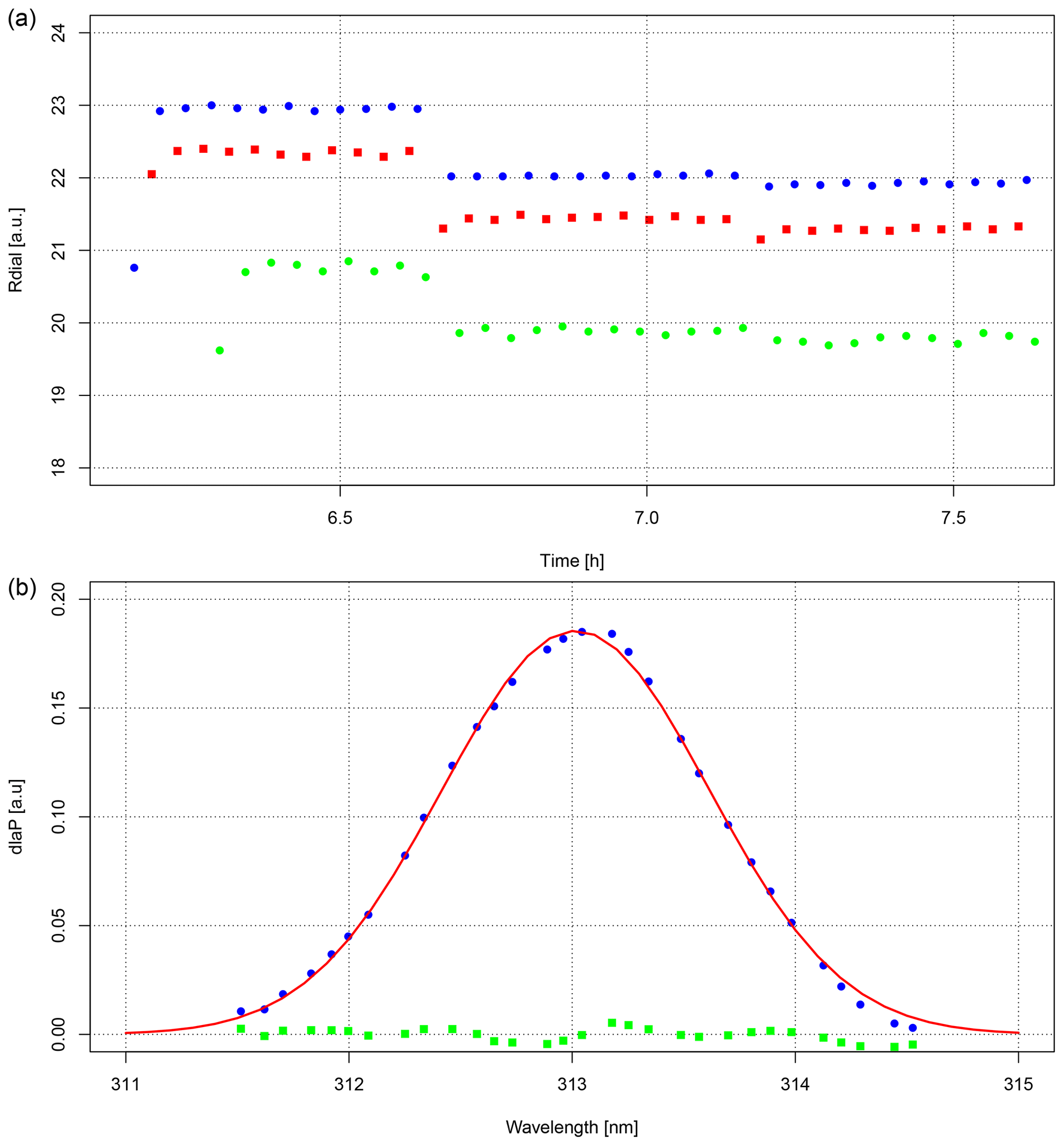
https://amt.copernicus.org/articles/14/5757/2021/amt-14-5757-2021-f06

Figure 6Results of semi-automatic standard lamp, that is, the Hg lamp tests of the Dobson D₀₆₂ instrument. (a) R-dial record of three different standard lamps for the wavelength pairs A (green), C (red) and D (blue). (b) PM dlaP response to the Q1 scan of the Hg lines at 312.96 nm: measured values (blue), fitted curve (red) and residuals (green).

Download

A Hg lamp is used to verify the wavelength settings and to check the optical alignment of the Dobson instrument. The test consists of scanning the 312.96 nm Hg spectral line through slit S2 by moving the Q1-lever wavelength selector (test S2Q1). Figure 6b shows the results of a Hg S2Q1 test with a Gaussian fit of the measurements. The calculated central value at 313.0 nm was in good agreement with the Hg spectral line, while the full width at half maximum (FWHM = 1.4 nm) is slightly larger than the measured values of 1.2 nm of Dobson instruments D₁₀₁ given in Table 1. In general, the tests consist of a succession of 10–20 scans to ensure a stable Hg lamp temperature. A deviation of the Hg test results from the nominal values requires an adaptation of the Q1 setting table and/or its temperature correction factor. Similarly, the test can be done by moving the Q2 instead of the Q1 lever (test S2Q2) or guiding the light through slit S3 instead of S2 (tests S3Q1 and S3Q2). Significant differences between the central position determined in each test are the sign of an optical misalignment of the instrument.

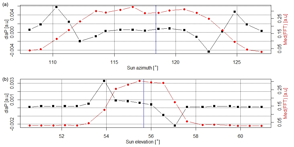
https://amt.copernicus.org/articles/14/5757/2021/amt-14-5757-2021-f07

Figure 7Results of the tests to control the sun azimuth and elevation. (a) dlaP signal (black) and FFT noise level (red) for a 20^∘ sun azimuth scan. The vertical blue line indicates the nominal value for a direct sun measurement. (b) Similar results for a 10^∘ sun elevation scan.

Download

Besides the lamp tests presented above that require the presence of the operator once a week, the DAQ system affords the possibility to check the behaviour of the instrument remotely. One of the key functions of the instrument control program is the tracking of the sun position, so two tests were implemented to scan the azimuth and elevation of the sun. Figure 7 illustrates results of these tests: the dlaP signal and the noise level were measured (5 s averages) at different azimuth (panel (a)) or elevation (panel (b)) angles. On both graphs, the nominal values, marked by the vertical blue lines, lie on the plateau part of both the dlaP and noise curves. These 2 min tests were realized close to local noon, allowing for a constant R-dial position. At other times of the day, a correction for the change of the R-dial value is necessary. The low values of the FFT noise level at both ends of the tests indicate that the entrance slit was not illuminated by the sun, while the flat part of the curves in the centre of the figures indicates full illumination. The parameters of these tests (averaging period, number of positions, scan interval, etc.) which can be adapted to local measurement conditions are stored in the configuration file.

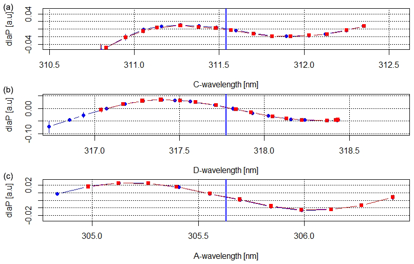
https://amt.copernicus.org/articles/14/5757/2021/amt-14-5757-2021-f08

Figure 8S-curve test results for the three wavelength pairs, (a) C, (b) D and (c) A. Nominal wavelengths are marked with the vertical blue lines at 311.5, 317.7 and 305.6 nm.

Download

Another test known as the “S-curve test” was described by G. B. W. Dobson in the Dobson instrument reference manual (revised version) (Evans, 2008). It checks the optical alignment of the instrument by scanning the solar irradiance around the nominal values of the three wavelength pairs. From the shape of the ozone absorption cross-section function, a symmetric response of the R-dial position is expected. A variation of this test was implemented in the DAQ system: the wavelength pairs are scanned simultaneously around the C, D and A nominal values. Around local noon, the R-dial positions corresponding to dlaP ≈ 0 do not change. Therefore from the locally linear relationship between the dlaP signal and the R-dial position, simultaneously scanning the Q1 and Q2 levers produces an S-curve response. G. B. W. Dobson reports the difficulty of obtaining a nice S curve for the C-wavelength pair and also the limited scanning range accessible for the D-wavelength pair. Examples of these S curves are shown in Fig. 8 for the three wavelengths pairs.

4 Discussion

The automation developed at MeteoSwiss has brought great benefits and flexibility to the use of the Dobson instrument. Besides the improvement of the data quality and measurement frequency discussed extensively in the paper by Stübi et al. (2021), the lifetime of these old instruments will be extended for years if not decades. This is an important perspective for long-term monitoring of climate-change-related parameters like the ozone column.

Other partial or full Dobson instrument automation projects have taken place since the 1970s (Räber, 1973; Malcorps and de Muer, 1977; Miyagawa, 1996; Komhyr et al., 1985; Kim et al., 1996). However, comprehensive descriptions of these developments in English are generally missing or not easily found in the open literature. A detailed comparison with the data acquisition scheme presented here is therefore not possible. The automated Dobson system developed by Miyagawa (1996) is the most widespread, as it has been installed at the NOAA's Dobson network stations (Evans et al., 2017). No major development of this system will probably take place as Japan is discontinuing its operational Dobson network. The Swiss automation system is unique in that the instruments are kept in a climatized container and are measuring through a quartz dome. This option prevents the exposure of the instrument to outside ambient conditions.

The continuous data recording allows relative daily variations to be followed as small as a fraction of a percent, which opens up possibilities to study variations on a timescale and with a measurement precision rarely achieved before with the Dobson instrument. The reproducible automated measurements could be used to develop advanced data treatment algorithms, taking into account the individual optical characteristics of the instruments (Gröbner et al., 2021). This could help to identify the origin of the systematic biases between the double wavelength pairs or to refine the treatment of the Rayleigh and/or Mie scattering terms.

The traditional standard lamp and Hg lamp tests could be fully automated by adapting a mechanism to slide the lamps into the sun director support. Such an option could be useful for remote sites like in the Arctic or Antarctic that are inaccessible for part of the year or to ease budgetary restrictions. Similarly, the option of automatically changing from zenith (Umkehr) to direct sun measurements could be automated using commercially available robotic arms to remove the sun director support.

Presently, most inversion algorithms for the Umkehr data to estimate the ozone profiles between 20 and 60 km altitude use only the C-wavelength measurements. An algorithm to include the combined information of the three wavelengths has been developed (Stone et al., 2014). The improved data reproducibility and quality of the automated Dobson instrument in combination with the reduced measurement uncertainty could be beneficial to optimize the information retrieved from the Umkehr inversion algorithm.

5 Conclusion

The automation of the control and of the data acquisition of Dobson sun spectrophotometers at MeteoSwiss has been a challenging development over the course of several years. Three Dobson instruments have been running in automated mode in Arosa and Davos without major problems for 5 years since the completion of the development phase. The short C–D–A measurement cycle of ∼ 150 s allows short-term ozone column variation to be followed at a resolution of ±1 DU in clear-sky conditions. The housekeeping data produced by the system, in particular the measure of the signal-to-noise associated with each measurement of the three wavelength pairs, has proven useful for the data quality control. This information may facilitate the advanced data processing and/or the inversion algorithms of Umkehr data. In the paper by Stübi et al. (2017 a), the results of the detailed analysis of the Arosa ozone column measurements with three automated Dobson instruments are presented.

Data availability

Operational ozone column data from Dobson D101 until 2014 and D062 from 2014 are available at WOUDC (https://woudc.org/home.php, Government of Canada, 2021) and NDACC (https://www-air.larc.nasa.gov/missions/ndacc/data.html#, NASA, 2021). For the extended set of housekeeping data, contact the corresponding author.

Author contributions

RS conducted the analysis of the data and wrote the first version of the manuscript. HS was in charge of the quality control and the preparation of the data sets. EMB, JK, HS and AH have contributed to the discussions and revisions of the manuscript.

Competing interests

The authors declare that they have no conflict of interest.

Disclaimer

Publisher’s note: Copernicus Publications remains neutral with regard to jurisdictional claims in published maps and institutional affiliations.

Acknowledgements

We would like to thank the PMOD/WRC staff for their great support in operating our instruments on their premises and for the excellent collaboration.

Review statement

This paper was edited by Mark Weber and reviewed by two anonymous referees.

References

Albrecht, F. and Parker, C. F.: Healing the Ozone Layer: The Montreal Protocol and the Lessons and Limits of a Global Governance Success Story, Oxford Scholarship Online Book, Great Policy Successes, edited by: 't Hart, P. and Compton, M., https://doi.org/10.1093/oso/9780198843719.003.0016, a

Basher, R. E.: Review of the Dobson spectrophotometer and its accuracy, WMO Global Ozone Research and Monitoring, Project, Report No. 13., Geneva, Switzerland, 1982. a

Breiland, J. G.: Vertical Distribution of atmospheric ozone and its relation to synoptic meteorological conditions, J. Geophys. Res., 69, 3801–3808, 1964. a

Brönnimann, S., Staehelin, J., Farmer, S. F. G., Cain, J. C., Svendry, T., and Svenøe, T.: Total ozone observations prior to the IGY. I: A history, Q. J. R. Meteorol. Soc., 129, 2797–2817, 2003. a

Christodoulakis, J., Varotsos, C., Cracknell, A. P., Tzanis, C., and Neofytos, A.: An assessment of the stray light in 25 years of Dobson total ozone data at Athens, Greece, Atmos. Meas. Tech., 8, 3037–3046, https://doi.org/10.5194/amt-8-3037-2015, 2015. a

Dobson, G. M. B.: Forty Years' Research on Atmospheric Ozone at Oxford: a History, Appl. Optics, 7, 387–405, 1968. a

Evans, R. D.: Operations Handbook–Ozone Observations with a Dobson Spectrophotometer, rev. ed., Rep. 183, Global Atmosphere Watch, World Meteorological Organization, Geneva, Switzerland, 2008. a, b, c

Evans, R. D., Petropavlovskikh, I., McClure-Begley, A., McConville, G., Quincy, D., and Miyagawa, K.: Technical note: The US Dobson station network data record prior to 2015, re-evaluation of NDACC and WOUDC archived records with WinDobson processing software, Atmos. Chem. Phys., 17, 12051–12070, https://doi.org/10.5194/acp-17-12051-2017, 2017. a, b

Fioletov, V. E., J. B. Kerr, C. T. McElroy, D. I. Wardle, V. Savastiouk, T. S. Grajnar: The Brewer reference triad, Geophys. Res. Lett., 32, L20805, https://doi.org/10.1029/2005GL024244, 2005. a

Government of Canada: World Ozone and Ultraviolet Radiation Data Centre, available at: https://woudc.org/home.php, last access: 2 August 2021. a

Gröbner, J., Redondas, A., Weber, M., and Bais, A.: Final report of the project Traceability for atmospheric total column ozone (ENV59, ATMOZ), EURAMET 2017, available at: https://www.euramet.org/research-innovation/search-research-projects/details/project/traceability-for-atmospheric-total-column-ozone/ (last access: 22 July 2021), 2017. a

Gröbner, J., Schill, H., Egli, L., and Stübi, R.: Consistency of total column ozone measurements between the Brewer and Dobson spectroradiometers of the LKO Arosa and PMOD/WRC Davos, Atmos. Meas. Tech., 14, 3319–3331, https://doi.org/10.5194/amt-14-3319-2021, 2021. a

Hoegger, B., Levrat, D., Staehelin, J., Schill, H., and Ribordy, P.: Recent developments of the Light Climatic Observatory–Ozone measuring station of the Swiss Meteorological Institute (LKO) at Arosa, J. Atmos. Terr. Phys., 54, 497–498, 1992. a

Kerr, J. B., McElroy, C. T., and Olafson, R. A.: Measurements of total ozone with the Brewer spectrophotometer, Proc. of the Quad. Ozone Symp., 4–9 August 1980, Boulder, CO, USA, edited by: London, J., Natl. Cent. for Atmos. Res., 74–79, 1981. a

Kim, J., Park, S. S., Moon, K.-J., Koo, J.-H, Lee, Y. G., Miyagawa, K., and Cho, H.-K.: Automation of Dobson Spectrophotometer (No.124) for Ozone Measurements, Atmosphere, 17, 339–348, 2007. a

Köhler, U., Nevas, S., McConville, G., Evans, R., Smid, M., Stanek, M., Redondas, A., and Schönenborn, F.: Optical characterisation of three reference Dobsons in the ATMOZ Project – verification of G. M. B. Dobson's original specifications, Atmos. Meas. Tech., 11, 1989–1999, https://doi.org/10.5194/amt-11-1989-2018, 2018. a, b

Komyhr, W. D.: Operations handbook – Ozone observations with a Dobson spectrophotometer, Global Ozone Research and Monitoring, Project Report 6, WMO, Geneva, Switzerland, 1980. a, b

Komhyr, W. D., Grass, R. D., Evans, R. D., Leonard, R. K., and Semeniuk, G. M.: Umkehr Observations with Automated Dobson Spectrophotometers, in: Atmospheric Ozone, edited by: Zerefos, C. S. and Ghazi, A., Springer, Dordrecht, Proceedings of the Quadrennial Ozone Symposium, 3–7 September 1984, Halkidiki, Greece, https://doi.org/10.1007/978-94-009-5313-0_75, 1985. a

Komhyr, W. D., Grass, R. D., and Leonard, R. K.: Dobson spectrophotometer 83: A standard for total ozone measurements, J. Geophys. Res., 94, 9847–9861, 1989. a, b, c

Malcorps, H., and de Muer, D.: Automation of a Dobson ozone spectrophotometer, Institut Royal Meteorologique de Belgique, Publications Série, 87, 1, Jan. 1977, available at: https://ui.adsabs.harvard.edu/abs/1977IRMBP..87....1M (last access: 22 July 2021), 1977. a

Mateer, C. L.: A study of the information content of Umkehr observations, PhD thesis, Univ. of Mich., Ann Arbor, USA, 1964. a

Miyagawa, K.: Development of automated measuring system for Dobson ozone spectrophotometer, in: XVIII Quadrennial Ozone Symposium, 12–21 September 1996, L’Aquila, Italy, vol. 2, edited by: Bojkov, R. and Visconti, G., 951–954, Int. Ozone Comm., 1996. a, b

Moeini, O., Vaziri Zanjani, Z., McElroy, C. T., Tarasick, D. W., Evans, R. D., Petropavlovskikh, I., and Feng, K.-H.: The effect of instrumental stray light on Brewer and Dobson total ozone measurements, Atmos. Meas. Tech., 12, 327–343, https://doi.org/10.5194/amt-12-327-2019, 2019. a, b

National Aeronautics and Space Administration (NASA): Network for the Detection of Atmospheric Composition Change (NDACC), available at: https://www-air.larc.nasa.gov/missions/ndacc/data.html#, last access: 2 August 2021. a

Perl, G. and Dütsch, H. U.: Die 30-jährige Aroser Ozonmessreihe, Ann. Schweiz. Meteor. Zentralanstalt, Nr. 8, 8.1–8.2, available at: https://www.meteosuisse.admin.ch/product/input/documents/annals/annalen-1958.pdf (last access: 22 July 2021), 1958. a

Petropavlovskikh, I., Bhartia, P. K., and DeLuisi, J.: New Umkehr ozone profile retrieval algorithm optimized for climatological studies, Geophys. Res. Lett., 32, L16808, https://doi.org/10.1029/2005GL023323, 2005. a

Räber, J. A.: An Automated Dobson Spectrophotometer, Pure Appl. Geophys., 106, 947–949, 1973. a, b

Redondas, A., Evans, R., Stuebi, R., Köhler, U., and Weber, M.: Evaluation of the use of five laboratory-determined ozone absorption cross sections in Brewer and Dobson retrieval algorithms, Atmos. Chem. Phys., 14, 1635–1648, https://doi.org/10.5194/acp-14-1635-2014, 2014. a

Scarnato, B., Staehelin, J., Stübi, R., and Schill, H.: Long-term total ozone observations at Arosa (Switzerland) with Dobson and Brewer instruments (1988–2007), J. Geophys. Res., 115, D13306, https://doi.org/10.1029/2009JD011908, 2010. a

Shaw, G. E.: Sun photometry, Bull. Am. Meteorol. Soc., 64, 4–10, 1983. a

Šmíd, M., Porrovecchio, G., Tesař, J., Burnitt, T., Egli, L., Grőbner, J., Linduška, P., and Staněk, M.: The design and development of a tuneable and portable radiation source for in situ spectrometer characterisation, Atmos. Meas. Tech., 14, 3573–3582, https://doi.org/10.5194/amt-14-3573-2021, 2021. a

Solomon, S.: Stratospheric ozone depletion: A review of concepts and history, Rev. Geophys., 37, 275–316, 1999. a

Solomon, S.: The discovery of the Antarctic ozone hole, Nature, 575, 46–47, https://doi.org/10.1038/d41586-019-02837-5, 2019. a

SPARC/IO3C/GAW: SPARC/IO3C/GAW Report on Long-term Ozone Trends and Uncertainties in the Stratosphere, edited by: Petropavloskick, I., Godin-Beekmann, S., Hubert, D., Damadeo, R., Hassler, B., and Sofieva, V., SPARC Report No. 9, GAW Report No. 241, WCRP-17/2018, https://doi.org/10.17874/f899e57a20b, 2019. a

Staehelin, J. and Viatte, P.: The Light Climatic Observatory Arosa: The story of the world’s longest atmospheric ozone measurements, Scientific Report MeteoSwiss and Institute of Atmospheric and Climate Science, 104, 243 pp. https://doi.org/10.18751/PMCH/SR/104.Ozon/1.0, 2019. a

Staehelin, J., Renaud, A., Bader, J., McPeters, R., Viatte, P., Hoegger, B., Bugnion, V., Giroud, M., and Schill, H.: Total ozone series at Arosa (Switzerland): Homogenization and data comparison, J. Geophys. Res., 103, 5827–5842, https://doi.org/10.1029/97JD02402, 1998. a

Staehelin, J., Viatte, P., Stübi, R., Tummon, F., and Peter, T.: Stratospheric ozone measurements at Arosa (Switzerland): history and scientific relevance, Atmos. Chem. Phys., 18, 6567–6584, https://doi.org/10.5194/acp-18-6567-2018, 2018. a

Stone, K., Tully, M. B., Rhodes, S. K., and Schofield, R.: A new Dobson Umkehr ozone profile retrieval method optimising information content and resolution, Atmos. Meas. Tech., 8, 1043–1053, https://doi.org/10.5194/amt-8-1043-2015, 2015. a

Stübi, R., Schill, H., Klausen, J., Vuilleumier, L., and Ruffieux, D.: Reproducibility of total ozone column monitoring by the Arosa Brewer spectrophotometer triad, J. Geophys. Res.-Atmos., 122, 4735–4745, https://doi.org/10.1002/2016JD025735, 2017a. a, b, c

Stübi, R., Schill, H., Klausen, J., Vuilleumier, L., Gröbner, J., Egli, L., and Ruffieux, D.: On the compatibility of Brewer total column ozone measurements in two adjacent valleys (Arosa and Davos) in the Swiss Alps, Atmos. Meas. Tech., 10, 4479–4490, https://doi.org/10.5194/amt-10-4479-2017, 2017b. a

Stübi, R., Schill, H., Maillard Barras, E., Klausen, J., and Haefele, A.: Quality assessment of Dobson spectrophotometers for ozone column measurements before and after automation at Arosa and Davos, Atmos. Meas. Tech., 14, 4203–4217, https://doi.org/10.5194/amt-14-4203-2021, 2021. a, b, c

WMO (World Meteorological Organization): Chapters 3 and 4 of Scientific Assessment of Ozone Depletion: 2018, Global Ozone Research and Monitoring Project–Report No. 58, Geneva, Switzerland, 588 pp., 2018. a

Articles

Short summary

In the first half of the 20th century, Prof. Dobson developed an instrument to measure the ozone column. Around 50 of these Dobson instruments, manufactured in the second half of the 20th century, are still used today to monitor the state of the ozone layer. Started in 1926, the Arosa series was, until recently, based on manually operated Dobsons. To ensure its future operation, a fully automated version of the Dobson has been developed. This well-working automated system is described here.