
Abstract
Music is a fundamental human construct, and harmony provides the building blocks of musical language. Using the Kunstderfuge corpus of classical music, we analyze the historical evolution of the richness of harmonic vocabulary of 76 classical composers, covering almost 6 centuries. Such corpus comprises about 9500 pieces, resulting in more than 5 million tokens of music codewords. The fulfilment of Heaps’ law for the relation between the size of the harmonic vocabulary of a composer (in codeword types) and the total length of his works (in codeword tokens), with an exponent around 0.35, allows us to define a relative measure of vocabulary richness that has a transparent interpretation. When coupled with the considered corpus, this measure allows us to quantify harmony richness across centuries, unveiling a clear increasing linear trend. In this way, we are able to rank the composers in terms of richness of vocabulary, in the same way as for other related metrics, such as entropy. We find that the latter is particularly highly correlated with our measure of richness. Our approach is not specific for music and can be applied to other systems built by tokens of different types, as for instance natural language.
1 Introduction
It is a well-known but nevertheless intriguing fact that the usage of natural language, as reflected in texts or speech, displays very strong statistical regularities [1–4]. Although the most popular and in-depth studied of these is Zipf’s law of word frequencies [5–9], the most fundamental linguistic statistical law is probably Heaps’ law, also called Herdan’s law [10–13]. This law relates the two main quantities that are necessary to set the statistical analysis of a text: the number of word tokens in the text, i.e., its length (in words), L, and the number of word types, which is referred to as the size of the vocabulary of the text, V. More precisely, Heaps’ law states that the relation between V and L is reasonably well approximated by a power law,
with an exponent \(\alpha \in (0,1]\) and a proportionality constant K.
Care has to be taken though when referring to Heaps’ law, as there are in fact two versions of it and considerable confusion between them. The first version deals, in principle, with just one text, and studies the growth of the accumulated vocabulary size as the text is read, from beginning to end. This yields a non-decreasing curve with no scattering that ends in the total values of vocabulary size and length for the considered text [14–16]. Although there are some derivations that relate this version of Heaps’ law with Zipf’s law, the situation is not so simple, and this version of Heaps’ law is usually a bad description of type-token growth, even if some formulation of Zipf’s law can be considered to hold [12, 17]. Instead of a linear trend in a log-log plot, what is usually observed is a slightly convex shape that has sometimes been confounded with a saturation effect [17].
The second version of Heaps’ law, the one considered in this study, needs a number of texts, or a collection of documents, and compares the total (final) values V and L for each one of the complete texts or documents. This results in a scatter plot, to which a power-law curve can be fitted to account for the correlation between V and L. This version of the law can be justified using the generalized central limit theorem [13], which has the advantage that does not require that Zipf’s law holds exactly, but only asymptotically. Overall, one must distinguish between an intra-text Heaps’ law (type-token growth) and an inter-text Heaps’ law (vocabulary-length correlation).
In practical applications, one is usually interested in quantifying attributes of the entities under study, and such quantification should be grounded on well-established statistical laws. In the case of natural language, there is an old tradition of evaluating richness of vocabulary [18], which has direct applications in authorship and genre analysis [19]. Comparing different texts (or authors), one could wrongly associate size of vocabulary V with richness of vocabulary. But the longer the text, the larger the vocabulary (on average), and texts of different length L cannot be compared in this way. One simple solution [20] is to divide the vocabulary size by the text length, yielding the so-called type-token ratio, \(V/L\).
Nonetheless, the fulfilment of Heaps’ law tells us that this linear rescaling is unjustified and, at the same time, suggests a natural solution. Several indices have been proposed following this reasoning (also as variations or alternatives to Heaps’ law [18]); for instance, Guiraud’s index,
or Herdan’s index,
The former assumes Heaps’ law with the “universal” value \(\alpha =0.5\) (and \(I_{G}=K\)), while the latter fixes \(K=1\) (with \(I_{H}=\alpha \)). The choice of \(K=1\) is naively justified by the obvious fact that \(V=1\) when \(L=1\); nevertheless, one should interpret Heaps’ law as a large-scale emergent property of texts that does not necessarily describe small-scale behavior. Note also that both indices are “absolute”, in the sense that they can be obtained for a single text or document (as one of the parameters of Heaps’s law, either K or α, are considered universal and fixed a priori).
As language, music is an attribute that defines us as humans [21]. A number of authors have pointed out similarities between language and music, and some have argued that music is indeed a “language” [22], although the notion of grammar and semantic content in music has been debated [21, 22]. Despite this, it is clear that there exist strong relations between language and music, specially regarding rhythm, pitch, syntax, and meaning [23]. This way, one can consider music as a succession (in time) of some musical symbols (which can be considered analogous to words in texts or speech), for which statistical analysis can be performed in the same way as in quantitative linguistics [24].
However, a remarkable problem is that, in contrast to language, the individual entities to analyze in music are not immediately clear [25]. For instance, Manaris et al. [26] mention diverse possibilities involving different combinations of pitch and duration, as well as pitch differences. This, together with some difficulties to deal with musical datasets in an automatized way, may explain the fact that the study of linguistic-like laws in music has been rather limited, in comparison with the study of natural language. Nevertheless, let us point out to Refs. [22, 27–30] as some of the pioneering analyses exploring the applicability of Zipf’s law in music (providing weak evidence in some cases).
In this paper, we deal with the suitability of statistical laws, in particular Heaps’ law, to describe regularities and patterns in musical pieces and to provide a natural metric to assess harmonic vocabulary richness. In contrast to previous metrics, this new one is not absolute, but relative to a given corpus or collection, as we argue that richness is more properly defined relative to an underlying probability distribution. Moreover, such relativeness yields a considerable advantage of interpretability of the obtained values. We also compare this metric with more common measures, finding that it is correlated with the entropy of the type-count distribution. To perform this research, we analyze classical music as captured by MIDI musical scores [31] and construct music codewords in a way similar to the one of Ref. [29].
In the next sections, we describe the extraction of music codewords from MIDI files (Sect. 2), overview the music corpus used (Sect. 2 too), present empirical results for Heaps’ law (Sect. 3), develop and apply our metrics for the quantification of vocabulary richness (Sect. 4), compare with entropy and codeword filling (Sect. 5), and test the robustness of the results in front of the criteria employed in codeword construction (Sect. 6). Naturally, we end with some discussion and conclusions (Sect. 7). Our work can be put in the context of culturomics, the rigorous quantitative inquiry of social sciences and the humanities by means of the analysis of big-data [32]. To facilitate assessment and future work on the topic, the code used in this paper is available at https://github.com/MarcSerraPeralta/chromagramer.
2 Processing and data
2.1 Construction of music codewords
In contrast to the famous composer Olivier Messiaen (and others), who considered rhythm as the essence of music, we put our focus on harmony, understood here simply as the combination of pitches (or, more precisely, pitch classes, as we will see immediately) for a given time frame. Our starting point are MIDI files, with each MIDI file corresponding to one electronic score of a musical piece (the corpus used is described at the end of this section). MIDI stands for Musical Instrument Digital Interface (for more information see the bibliography in Refs. [31, 33]).
One might complain that audio recordings are richer than MIDI files as expressions of music, as the latter may lack the variability and nuances of interpretation [34] (some other MIDI files may additionally not correspond to “original” scores, but are created from the life performance of a musical piece). However, we may argue that a musical score contains the core of a piece. As we will need to discretize the elements that form the pieces, scores provide an objective first step in such discretization. The situation may be considered similar to the relation between written language and speech [3, 35]. Moreover, as no original recordings exist for classical music (except for the last 100 years or so), scores are our best link with the spirit of the composer.
The procedure to obtain elementary units (codewords) from MIDI files is the following (similar to the one in Ref. [29], and illustrated in Fig. 1):
-
First, MIDI files are read using the program midi2abc [36] and converted into standard text files containing the onset time, duration, and pitch of each note. Pitches range from C-1 (fundamental frequency at 8.1758 Hz), MIDI note 0, to G9 (12,543.85 Hz), MIDI note 127. A4 (440 Hz) is MIDI note 69. For some pieces starting and/or ending with silences (empty bars or beats), these are removed, in order to avoid an artificial overestimation of L. The files also contain metadata about the key of the pieces, which we disregard (due to some unreliability we found in some control checks in the corpus we used).
-
With the purpose of reducing dimensionality, all notes are collapsed into a single octave, i.e., the pitches A0, A1, A2, etc., are considered to be the same note, or pitch class, A (or la, in solfège notation), and the same for the rest of pitches. This leads to 12 pitch classes. This dimensional reduction has also a perceptual basis, rooted on the prevalence of the Western reference system based on the octave [21, 37].
-
In order to decrease temporal resolution, each score is divided into small discrete time frames. By default, we chose this time unit to be the beat (as this is probably the most relevant time scale in music [21]). For example, the \({}^{4}_{4}\) bar yields 4 beats per bar, whereas the \({}^{3}_{8}\) bar yields 3.
-
For each time frame we construct a 12-dimensional vector, with one component for each pitch class, \(C,C\#,\dots G\#, A,A\#,B\), i.e., from do to si. Each component of the vector contains the sum of all durations of notes of the corresponding pitch class in the corresponding time frame. All notes coming from different instruments (or different pentagrams) playing in parallel are counted at a given time frame (as seen in Fig. 1), due to the fact that they are perceived together by the listener. In this way, if the unit is the beat, in the \({}^{4}_{4}\) bar, each quarter note or crotchet counts as one, and each eighth note or quaver counts as one half, whereas in the \({}^{3}_{8}\) bar, it is the eighth note which counts as one. Notes that occupy more than one time frame are split according to their duration in each of them (and thus, the maximum contribution coming from an individual note in the score is one at each time frame). The vectors obtained in this way are called chromas.
Figure 1 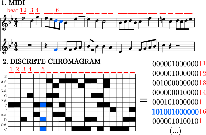
Example of a sequence of discretized chromas (chromagram) arising from a MIDI score. Note that the two pentagrams constituting the score have to be read in parallel
-
To further simplify, and in order to get well defined countable entities, chroma vectors are discretized, with components below a fixed threshold (0.1 by default) reset to zero and components above the threshold reassigned to one. In this way, a value equal to one in a component of the discretized vector means that the corresponding pitch class has a significant presence (above 0.1) in that time frame, whereas a value of zero means that the pitch class has null or very little weight and can be disregarded. We refer to the resulting discretized vectors as discretized chromas.

Note that the procedure of codeword construction has just two parameters: the time unit, which we take to be the beat, and the discretization threshold, which we have equated to 0.1. These values can be considered somewhat arbitrary (in particular the threshold). Therefore, to demonstrate the generality of our approach, we also test the robustness of our results in front of different prescriptions for them (Sect. 6).
Discretized chromas constitute our music codewords, and turn out to be nothing else than 12-digit binary numbers (from 0 to \(2^{12}-1=4095\), which also represent the vertices of a 12-dimensional hyper-cube). One could argue that these entities would be closer to music letters than to music words; however, previous statistical analysis [29] shows that the complexity contained in them is enough to treat them as music words. Further, our codewords have “temporal structure”, as they can be composed by the succession of several shorter notes (for example, in the \({}^{3}_{4}\) bar, the duration of one beat is that of two consecutive quavers, or four semiquavers, etc.). Perhaps, the fundamental difference with words is that our music codewords have a fixed length (that of the selected time unit), whereas in linguistics the length of words is variable (given by the number of letters, for instance) and determinant for the validity of Zipf’s law [4].
2.2 Transposition
An additional step of the procedure is to transpose all pieces to a common key, so that all major keys are transposed to C major and all minor ones to A minor (the reason of using A minor instead of C minor is that the former is the relative minor of C major, sharing the same key signature and leading thus to a more similar usage of chromas). For example, if a piece is in G major, all G pitches in the piece are transformed to C pitch class, all G# pitches to C#, and so on. This is just a shift in pitch-class space. Although keys are directly provided by the MIDI file (at least for the majority of files), an initial inspection showed that this information is unreliable, and thus we perform our own analysis of key (see Appendix B for details). No attempt is performed to identify changes of key inside a piece, so we calculate the predominant or more common key for each piece.
If a piece keeps a constant key, transposition has no influence on the size of its vocabulary, but if different pieces are merged into a single dataset (as we will do), it can be convenient to merge them after they are transposed to the same key. In this case, if the pieces come in different keys, transposition leads obviously to a different vocabulary, where one does not deal with pitch classes but with tonal function (and thus, the resulting C pitch class represents the tonic, G represents the dominant, etc. [38, 39]). Transposition can be useful also to unveil a reduced vocabulary, where a given composer could show what seems a broad apparent richness that arises from a limited vocabulary transposed into a number of different keys.
In some sense, for listeners with absolute pitch [21], it makes sense to keep the original key of different pieces when they are merged to form a larger dataset (these listeners naturally distinguish the different pitches and also the keys). However, for the vast majority of listeners (those with relative pitch), it is more natural to merge pieces while transposing to a fixed key (at least in the usual equal-temperament tuning system [21]). For this reason, we will only work with transposed pieces in our analysis.
2.3 Concatenation and elementary statistics
As we are particularly interested in studying individual composers, we concatenate all the pieces corresponding to the same composer into a single dataset. Each dataset turns out to be constituted by a succession of discretized chromas. Each repetition of a particular discretized chroma is a token of the corresponding codeword type. The number of different types in the dataset (the types with absolute frequency greater than zero) is then the vocabulary size, denoted by V (this number will be smaller than 4096, in practice). The sum of all the absolute frequencies of all types yields the total number of tokens, which corresponds, by construction, to the dataset length L measured in number of the selected time units. In a formula, \(\sum_{r=1}^{V} n_{r} =L\), where r labels all the codeword types in the dataset and \(n_{r}\) denotes the absolute frequency of type r.
2.4 Musical corpus
We perform our study over the Kunstderfuge corpus [40], which, at the time of our analysis, consisted of 17,418 MIDI files corresponding to pieces of 79 classical composers, from the 12th to the 20th century (Ref. [41] has scrutinized the Kunstderfuge corpus looking for properties different than the ones we are interested in). Removing files that were not clearly labelled or corrupted (files that we are not able to process) and files for which we could not obtain the bar (and thefore could not determine the beat), yields a remainder of 9489 files and 76 composers, ranging from Guillaume Dufay (1397–1474) to Messiaen (1908–1992). The names of all composers are provided in Table 1 (Appendix A). The total length of the resulting corpus is \(L=5\text{,}131\text{,}159\) tokens, with a total vocabulary \(V=4085\).
Figure 2(a) shows, for each piece, its length L and the size of its vocabulary V, by means of the corresponding distributions (probability mass functions \(f(L)\) and \(f(V)\)). Both L and V show a variability of around three orders of magnitude, with a maximum (i.e., a mode) around 100 tokens for L and 50 types for V. The distributions of L and V would correspond to intrinsic properties of classical musical compositions, which can nevertheless be biased due to subjective or arbitrary criteria employed when creating the Kunstderfuge corpus.

As mentioned, for statistical purposes we aggregate all the compositions by the same author into a single dataset for that author. Figure 2(b) does the same job for authors as Fig. 2(a) was doing for single pieces. Since L is a purely additive quantity (by definition of token), the values of L increase when going from pieces to authors, but the variability of three orders of magnitude is more or less maintained. The tail of \(f(L)\) can be fitted by a decreasing power law, with an exponent around 1.95, although the number of data points (composers) in the tail is small. (in Ref. [9], a power-law tail with an exponent close 3 was proposed for the distribution of text lengths, but for individual written works, i.e., without author aggregation). In contrast to L, the size of vocabulary V decreases its variability when going from pieces to composers, as types are not additive. The distributions \(f(L)\) and \(f(V)\) at the author level do not show any musical characteristic, as we expect them to be incomplete, in principle (not all the pieces from each author are present in Kunstderfuge). So, they characterize the corpus, and not the creativity of the composers.
3 Fulfilment of Heaps’ law
As an illustration of the data we deal with, we report in Table 2 (in Appendix A) the values of length L and size of vocabulary V for the 15 composers with the largest values of V, as derived from the Kunstderfuge corpus. All of them turn out to be very well-known composers, except perhaps Ferruccio Busoni (an Italian virtuoso pianist). The top-3 most represented composers in terms of length L are Bach, Beethoven, and Mozart, with \(L\simeq 760\), 670, and 500 thousand tokens, respectively. Figure 3(a) shows the corresponding scatter plot for all 76 composers. The average increase of V with L is apparent, but with considerable scattering.

(a) Scatter plot of size of vocabulary versus number of tokens (length) for the 76 composers in the corpus, who are grouped chronologically, as represented by the points of different color (one point is one composer). The year of each composer is the mean between the birth year plus 20 and the death year. Heaps’ law is given by the central straight line and the parallel lines denote one standard deviation \(\sigma _{c}\). Notice that when a limited chronological span is considered, the scattering is reduced. (b) Analog scatter plot for the 9489 individual pieces. Year of a piece is approximated to the year of its composer. The results of the fits are in Table 3 (in Appendix A)
In order to obtain the parameters of Heaps’ law, we fit a regression line to the relation between logV and logL, from which we obtain a Heaps’ exponent \(\alpha \simeq 0.35\), with a linear (Pearson) correlation coefficient \(\rho \simeq 0.64\) (the value of log10K turns out to be 1.47). All the results of the fit are available in Table 3 (Appendix A), and the resulting power law is represented in Fig. 3. For completeness, we perform the same power-law fit for individual pieces, see Fig. 3(b). The results, also in Table 3, show a much higher exponent, \(\alpha \simeq 0.66\) (clearly above 0.5 this time), and also a higher linear correlation coefficient, \(\rho \simeq 0.85\).
Thus, the supposedly universal values of α and K for texts mentioned in the introduction (either \(\alpha =0.5\) or \(K=1\) [18]) clearly do not hold for music, at least at the level of composers. In any case, it is apparent that the larger the value of L, the larger (on average) the vocabulary size, but the increase in V is rather modest, due to the small value of the exponent α (in other words, we need a 7 times longer piece for seeing a doubling of the vocabulary size). The relative large value of the constant K reported above for the composers arises as a compensation for the small value of α.
4 Richness of vocabulary
Due to the existence of Heaps’ relation between V and L, as explained in the introduction, it is erroneous to identify vocabulary size with vocabulary richness. For each composer, Heaps’ law provides a natural way to correct the changes in V due to the heterogeneities and biases in L. We have also mentioned how the Giraud’s and Herdan’s indices are based on supposedly universal properties of Heaps’ law. However, notice that in the case of music, such universal properties do not hold anymore, as \(\alpha \ne 0.5\) and \(K\ne 1\).
Therefore, we develop here a measurement of richness based on the empirical (non-universal) validity of Heaps’ law, which will be relative to the rest of authors in a given corpus. In short, composers (or datasets, in general) with V above the “regression line” in the scatter plot (for the corresponding value of L) will have a vocabulary richness greater than what the Heaps’ power law predicts, whereas composers below it will have lower richness.
Thus, we will calculate the difference \(\log _{10} V - \log _{10} K -\alpha \log _{10} L\) from the empirical data (using the fitted values of K and α), and will rescale the result in “units” of \(\sigma _{c} = \sigma _{y} \sqrt{1-\rho ^{2}}\), as the theory of linear regression tells us that the standard deviation of log10V at fixed L is \(\sigma _{c}\), with \(\sigma _{y}\) the standard deviation of log10V for all values of L. So, the vocabulary relative richness R of each composer is defined as
With that, \(R>0\) will correspond to high vocabulary richness (higher than average) whereas \(R<0\) is, obviously, negative richness, i.e., poverty of vocabulary. This easiness of interpretation of our relative richness is an additional advantage in comparison to the indices of richness \(I_{G}\) and \(I_{H}\), whose values are not directly interpretable. The rescaling of the logarithm in terms of \(\sigma _{c}\) in Eq. (1) is not necessary if we deal with a single corpus (as it is the case here), but could be useful to compare different corpora or even different phenomena, such as musical richness with literary richness. Rescaling also provides further interpretability for the values of R, in terms of standard deviations from the mean (in logarithmic scale).
When applied to our data, the composer with highest value of R turns out to be Paul Hindemith (\(R=1.68\)), closely followed by Serguéi Rajmáninov (with nearly the same R). The lowest R corresponds to Tomás Luis de Victoria (\(R=-2.49\)). In Table 4 (Appendix A) we provide some more details on the ranking of composers by different metrics. General information on these composers can be found in Table 5 (Appendix A).
Interestingly, the chronological display in Fig. 4 of the relative richness R of each composer shows a clear increasing trend of this richness across the centuries, with a linear-slope increase of 0.72 “units of richness” per century (and linear correlation coefficient \(\rho =0.90\)). It is interesting to note that Ref. [29] reported a decreasing trend for contemporary Western popular music; nevertheless, it should be also noted that, besides the different genres and epochs, richness was measured by modeling transitions between codewords using a complex network approach. Figure 5 compares our relative richness R, for each composer, with the logarithms of other composers’ characteristics (L, V, type-token ratio, \(I_{G}\), etc.). Figure 5(a) shows all pairs of scatter plots between the metrics of the composers and Fig. 5(b) shows the corresponding matrix of linear correlation coefficients. The high correlation between the relative richness and the year of each composer is apparent (below we will discuss this figure in more detail).

Vocabulary relative richness R for each composer in chronological order. Horizontal axis is birth \(+\, 20\, +\) death, divided by 2. The straight line is a linear regression with slope \(0.72\pm 0.04\) “units of richness” per century and a linear correlation coefficient \(\rho =0.90\) (and intercept −12.9). Some particular composers are highlighted, for the sake of illustration

Comparison of the different metrics characterizing each composer. (a) Scatter plots. (b) Matrix of linear correlation coefficients
5 Comparison with entropy and filling of codewords
A quantity of relevance in this context is the entropy of the distribution of type frequency [44]. Each codeword type r (with \(r=1,2,\dots, V\)) has a relative frequency given by its number of tokens divided by L, which we can assimilate to the probability of the type \(P_{r}\) in the selected dataset, which in our case corresponds to individual composers. The Shannon entropy (in bits) characterizing the vocabulary of each composer is simply
In the hypothetical (unrealistic) case of uniform use of all possible types, V would reach its maximum value, 212, and we would obtain the maximum possible entropy, \(S_{\mathrm{max}}=\log _{2} 2^{12}=12\) bits.
In our composers’ corpus, the highest entropy is given by Stravinsky (\(S=9.95\) bits), followed by Gustav Mahler (\(S=9.91\) bits). The lowest value of entropy corresponds to Orlande de Lassus (or Orlando di Lasso, with S around 5.8 bits). We see that, as in the relative richness, the composers with the lowest entropies are from the 15th or 16th centuries, whereas those with the highest entropies are from the end of the 19th or the 20th century. The systematic increase of the entropy when the composers are ordered chronologically is analogous to the increase shown in Fig. 4. Linear regression shows that the increase in entropy is 0.69 bits per century (with a linear correlation coefficient equal to 0.83). Thus, the history of classical music (on average) seems to extend the law of the increase of entropy with time beyond the usual physical systems considered in thermodynamics [45]. The comparison of the entropy with the other metrics is included in Fig. 5.
Finally, another metric of potential interest is the average filling of the codeword types for each composer, calculated as \(\langle F \rangle = \sum_{r=1}^{V} P_{r} F_{r}\), with \(F_{r}\) the number of ones in the discretized chroma corresponding to codeword type r (if the codeword r is represented as a 12-component vector, then \(F_{r}=\sum_{i=0}^{11} r_{i}\), with \(r_{i}\) the i-th component of the vector r, taking values \(r_{i}=0\) or 1, as we have defined). The composer with more average filling is Nikolai Medtner (\(\langle F\rangle =4.46\)), and the one with less value is Niccolò Paganini (the most ancient composer in the corpus, with \(\langle F\rangle =2.62\)). This metric also shows an increasing trend across the years, but, in contrast to R and S, its correlation with time is not high. The scatter plot, included in Fig. 5(a), has an upper envelope that increases linearly in time, but the lower envelope is rather constant. In this way, Messiaen (the most modern composer included in the corpus), shows one of the lowest values of \(\langle F \rangle \). The average filling is compared with the rest of metrics also in Fig. 5(b), where we see that it is not very highly correlated with any of them.
6 Robustness of results
We have tested the robustness of our results in front of the arbitrariness contained in the process of codeword construction. For that purpose, we have investigated the effect of changing the value of the discretization threshold. We find that thresholds ranging from 0.025 to 0.2 lead to very minor changes of the Heaps’ exponent α, with values comprised between 0.350 and 0.355. A threshold equal to zero leads to α around 0.355. Thresholds higher than 0.3 lead to progressively increasing α, e.g., for 0.5 we get \(\alpha \simeq 0.39\). The intercept in Heaps’ regression (K) shows higher variability; nevertheless, although the specific values of the relative richness R depend on K, their statistical properties do not change (as K is only bringing a shift in logarithmic scale). The stability of α ensures the robustness of R.
We have also explored the effects of changing the time unit over which the codewords are built, finding that an increase in the time unit from 0.5 to 1.5 beats leads to a modest increase in α from 0.33 to 0.39 (with very little influence in the value of the threshold, in the same way as explained above). Taking a time unit as large as 4 beats leads to α close to 0.5. This is a considerable change, but not unexpected, as, for instance, in a \({}^{4}_{4}\) bar, 4 beats correspond to one bar and conventional musical knowledge tells us that bar-based codewords are entities with different properties than beat-based codewords.
7 Summary and discussion
Summarizing the results, the highest linear correlation between all the metrics characterizing the composers is the one relating the relative richness R with the entropy (around 0.95, Fig. 5(b)), but R is also highly correlated with the Giraud index. The Herdan index is also highly correlated with Giraud and with the type-token ratio. The correlations obtained between \(\langle F\rangle \) and the other indices are not so high. Interestingly, the highest correlation of the year characterizing each composer is with the proposed relative richness R (taking a value of 0.90, Fig. 5(b)). The correlation of R with logL is zero by construction. Replacing Pearson linear correlation with Spearman or Kendall correlations does not qualitatively change very much this pattern of correlations (not shown).
So, we conclude that relative richness presents very interesting properties, as it shows maximum correlation with entropy and with year. Nevertheless, the correlation of relative richness with entropy is so high that one could consider instead to use entropy to account for vocabulary richness. This has the advantage that one does not need to have a whole corpus to obtain the Heaps’ law in advance; rather, it can be calculated even for a single author or piece, or it can be used for the comparison of just two authors. Nonetheless, the entropy has the disadvantage that one does not know what a high entropy or a low entropy is, in principle, and thus, the apparent advantage of entropy is lost in a practical situation. Interpretability is further hampered by not having a direct notion of “above/below average” richness, which is corpus dependent. From the comparison with the relative richness we see that the value of S separating low richness and high richness is around 8 bits (for the present codification of 12 bits per codeword and for the present corpus). Very low richness is around 6 bits and very high around 10. This also corresponds to an average filling of codewords (mean number of ones) ranging from 2.7 to 4.5. Another disadvantage of entropy is that one needs to count the repetitions of all codeword types (the V values of \(P_{r}\)), whereas for the richness one only needs to know how many types there are (the value of V).
In conclusion, we have analyzed the harmonic content of a large corpus of classical music in MIDI form. The definition of music codewords allows us to quantify the size of the harmonic vocabulary of classical composers, and relate it to their musical productivity (the total length of their compositions, as contained in the considered corpus). We obtain that the relation between the two variables is well described by an increasing power law, which is analogous to the Heaps’ law previously found in linguistics and other Zipfian-like systems. Nevertheless, the obtained power-law exponent turns out to be somewhat small (\(\alpha \simeq 0.35\)), if we compare it to typical values found in linguistics.
Heaps’ law allows us to develop a proper measure of vocabulary richness for each composer in relation to the rest of the corpus. Remarkably, we find that vocabulary richness undergoes a clear increasing trend across the history of music, as expected from qualitative musical wisdom. Our approach provides a transparent quantification of this phenomenon. We also show that our relative richness is highly correlated with the entropy of the distribution of codeword frequencies, so entropy can be equally used to measure vocabulary richness, once it is properly calibrated. Our metric has several advantages with respect to previous indices of richness, such as being relative to the richness of the rest of composers and a better interpretability of the values. At our level of resolution (that of individual composers) the evolution of richness does not show any revolutions or sudden jumps; instead, it seems to be rather gradual, and well fitted by a linear increase. (the variability is too high to allow one to obtain meaningful results beyond the linear increasing trend).
Availability of data and materials
The data that support the findings of this study are available from kunstderfuge.com but restrictions apply to the availability of these data, which were used under license for the current study, and so are not publicly available.
References
Altmann EG, Gerlach M (2016) Statistical laws in linguistics. In: Creativity and universality in language. Springer, Cham, pp 7–26
Hernández T, Ferrer i Cancho R (2019) Lingüística cuantitativa, Madrid
Torre IG, Luque B, Lacasa L, Kello CT, Hernández-Fernández A (2019) On the physical origin of linguistic laws and lognormality in speech. R Soc Open Sci 6(8):191023
Corral Á, Serra I (2020) The brevity law as a scaling law, and a possible origin of Zipf’s law for word frequencies. Entropy 22(2):224
Baayen RH (2002) Word frequency distributions, vol 18. Springer, Dordrecht
Kytö M, Lüdeling A (2009) Corpus linguistics: an international handbook. de Gruyter, Berlin
Zanette DH (2014) Statistical patterns in written language. Preprint. arXiv:1412.3336
Piantadosi ST (2014) Zipf’s word frequency law in natural language: a critical review and future directions. Psychon Bull Rev 21(5):1112–1130
Moreno-Sánchez I, Font-Clos F, Corral Á (2016) Large-scale analysis of Zipf’s law in English texts. PLoS ONE 11(1):0147073
Baeza-Yates R, Ribeiro-Neto B et al. (1999) Modern information retrieval, vol 463. ACM, New York
Kornai A (2002) How many words are there? Glottometrics 4:61–86
Font-Clos F, Boleda G, Corral A (2013) A scaling law beyond Zipf’s law and its relation to heaps’ law. New J Phys 15(9):093033
Corral Á, Font-Clos F (2017) Dependence of exponents on text length versus finite-size scaling for word-frequency distributions. Phys Rev E 96(2):022318
Mandelbrot B (1961) On the theory of word frequencies and on related markovian models of discourse. In: Structure of language and its mathematical aspects, vol 12. Am. Math. Soc., Providence, pp 190–219
Heaps HS (1978) Information retrieval, computational and theoretical aspects. Academic Press, San Diego
Serrano MÁ, Flammini A, Menczer F (2009) Modeling statistical properties of written text. PLoS ONE 4(4):5372
Font-Clos F, Corral Á (2015) Log-log convexity of type-token growth in Zipf’s systems. Phys Rev Lett 114(23):238701
Wimmer G, Altmann G (1999) On vocabulary richness. J Quant Linguist 6(1):1–9
Kubát M, Milička J (2013) Vocabulary richness measure in genres. J Quant Linguist 20(4):339–349
Richards B (1987) Type/token ratios: what do they really tell us? J Child Lang 14(2):201–209
Ball P (2010) The music instinct. Oxford University Press, Oxford
Zanette DH (2006) Zipf’s law and the creation of musical context. Music Sci 10(1):3–18
Patel AD (2010) Music, language, and the brain. Oxford University Press, Oxford
Zanette D (2008) Playing by numbers. Nature 453(7198):988–989
Corral Á, Boleda G, Ferrer-i-Cancho R (2015) Zipf’s law for word frequencies: word forms versus lemmas in long texts. PLoS ONE 10(7):0129031
Manaris B, Purewal T, McCormick C (2002) Progress towards recognizing and classifying beautiful music with computers-midi-encoded music and the Zipf–Mandelbrot law. In: Proceedings IEEE SoutheastCon 2002 (Cat. No. 02CH37283). IEEE Press, New York, pp 52–57
del Río MB, Cocho G, Naumis G (2008) Universality in the tail of musical note rank distribution. Phys A, Stat Mech Appl 387(22):5552–5560
Haro M, Serrà J, Herrera P, Corral Á (2012) Zipf’s law in short-time timbral codings of speech, music, and environmental sound signals. PLoS ONE 7(3):33993
Serrà J, Corral Á, Boguñá M, Haro M, Arcos JL (2012) Measuring the evolution of contemporary western popular music. Sci Rep 2(1):1–6
Liu L, Wei J, Zhang H, Xin J, Huang J (2013) A statistical physics view of pitch fluctuations in the classical music from bach to chopin: evidence for scaling. PLoS ONE 8(3):58710
Wikipedia: MIDI. https://en.wikipedia.org/wiki/MIDI. Accessed 20 Feb 2021
Michel J-B, Shen YK, Aiden AP, Veres A, Gray MK, Pickett JP, Hoiberg D, Clancy D, Norvig P, Orwant J et al. (2011) Quantitative analysis of culture using millions of digitized books. Science 331(6014):176–182
Benson D (2006) Music: a mathematical offering. Cambridge University Press, Cambridge
Hennig H, Fleischmann R, Geisel T (2012) Musical rhythms: the science of being slightly off. Phys Today 65(7):64
Torre IG, Luque B, Lacasa L, Luque J, Hernández-Fernández A (2017) Emergence of linguistic laws in human voice. Sci Rep 7(1):1–10
midi2abc: abcMIDI package. http://abc.sourceforge.net/abcMIDI/original. Accessed 20 Feb 2021
Krumhansl CL, Kessler EJ (1982) Tracing the dynamic changes in perceived tonal organization in a spatial representation of musical keys. Psychol Rev 89(4):334
Press OU Grove music online. https://www.oxfordmusiconline.com/grovemusic. Accessed 28 Feb 2021
Pilhofer M, Day H (2015) Music theory for dummies. Wiley, New York
Kunstderfuge: the largest resouce of classical music in .mid files. http://www.kunstderfuge.com. Accessed 1 Feb 2021
González-Espinoza A, Martínez-Mekler G, Lacasa L (2020) Arrow of time across five centuries of classical music. Phys Rev Res 2(3):033166
Deluca A, Corral Á (2013) Fitting and goodness-of-fit test of non-truncated and truncated power-law distributions. Acta Geophys 61(6):1351–1394
Corral Á, González Á (2019) Power law size distributions in geoscience revisited. Earth Space Sci 6(5):673–697
Corral Á, Serra I, Ferrer-i-Cancho R (2020) Distinct flavors of Zipf’s law and its maximum likelihood fitting: rank-size and size-distribution representations. Phys Rev E 102(5):052113
Ben-Naim A (2019) Entropy and information theory: uses and misuses. Entropy 21(12):1170
Temperley D (1999) What’s key for key? The Krumhansl–Schmuckler key-finding algorithm reconsidered. Music Percept 17(1):65–100
Krumhansl CL, Cuddy LL (2010) A theory of tonal hierarchies in music. In: Music perception. Springer, New York, pp 51–87
Acknowledgements
Some preliminary work of this project was done by I. Moreno-Sánchez, funded by the Collaborative Mathematics Project of the La Caixa Foundation. Also, M. S.-P.’s participation has been possible thanks to the Internship Program of the Centre de Recerca Matemàtica.
Funding
Support from projects FIS2015-71851-P and PGC-FIS2018-099629-B-I00 from Spanish MINECO and MICINN is acknowledged.
Author information
Authors and Affiliations
Contributions
MS-P wrote the code and analyzed the data, JS and AC supervised the results, all authors interpreted the results. AC wrote the first draft of the manuscript and all authors revised the manuscript. All authors read and approved the final manuscript.
Corresponding author
Ethics declarations
Competing interests
The authors declare that they have no competing interests.
Appendices
Appendix A: Tables
In this appendix we include the tables cited in the text. Table 1 contains the names of the 76 composers in the corpus, in chronological order. Table 2 provides the values of L and V (together with other relevant figures) for the 15 composers best represented (in terms of V) in the corpus. Table 3 yields the results of fitting Heaps’ law to the values of V and L for the individual composers and for the individual pieces. The results for the composers without performing any transposition are also included, for the sake of comparison. Observe how the exponent α remains essentially the same. Table 4 shows the top-5, medium-6, and bottom-5 composers regarding relative richness, entropy, and average filling. Table 5 gives the general details of the composers highlighted in the previous table.
Appendix B: Transposition procedure
The method we use for the analysis of the key is the Krumhansl-Schmuckler Key-Finding Algorithm [46]. This algorithm is based on the key profiles described in Ref. [37], which were obtained by empirical experiments where subjects rated how well each pitch fitted a prior context establishing a key. The values for the major key profile are 6.35, 2.23, 3.48, 2.33, 4.38, 4.09, 2.52, 5.19, 2.39, 3.66, 2.29 and 2.88, where the first number corresponds to the mean rating for the tonic of the key, the second to the next of the 12 tones in the chromatic scale, etc. The values for the minor key context are 6.33, 2.68, 3.52, 5.38, 2.60, 3.53, 2.54, 4.75, 3.98, 2.69, 3.34 and 3.17 [47].
The procedure of the algorithm to calculate the key of a piece is as follows:
-
1.
Average, in terms of tokens, the discretized chromas in the considered piece.
-
2.
Calculate the Pearson linear correlation of the major key profiles with the average discretized chroma and all their circular shifts (12 values).
-
3.
Repeat step 2 using the minor key profiles.
-
4.
The transposition shift is the shift that maximizes the correlation from both steps 2 and 3.
The key is obtained directly from the transposition shift, with the following correspondence: \(0 = C\), \(1 = C\#/D\flat \), \(2 = D\), \(3 = D\#/E\flat \) … For the Kunstderfuge corpus we find that the most common keys are G Major, C Major, and D minor, as shown in Fig. 6, whereas the least common are E♭ minor and B♭ minor.

Absolute abundance of each key in the corpus, counted in number of pieces, before transposition, obviously. Zero corresponds to C Major, one to C#/D♭ Major… up to B Major; 20 corresponds to C minor and so on
We do not use the information about the key provided by the metadata in the MIDI file, as this seems to refer to the key signature rather than to the key. To check that the transposition is being done correctly, we verify that the most common codewords after transposition are CEG, CFA, CEA, DGB, and the empty codeword, corresponding to a silent beat. Table 6 shows the top 10 codewords, in terms of absolute frequency, making clear how these can be related to chords or tonal functions that are common in C major or A minor. in C Major or A minor.
Rights and permissions
Open Access This article is licensed under a Creative Commons Attribution 4.0 International License, which permits use, sharing, adaptation, distribution and reproduction in any medium or format, as long as you give appropriate credit to the original author(s) and the source, provide a link to the Creative Commons licence, and indicate if changes were made. The images or other third party material in this article are included in the article’s Creative Commons licence, unless indicated otherwise in a credit line to the material. If material is not included in the article’s Creative Commons licence and your intended use is not permitted by statutory regulation or exceeds the permitted use, you will need to obtain permission directly from the copyright holder. To view a copy of this licence, visit http://creativecommons.org/licenses/by/4.0/.
About this article

Cite this article
Serra-Peralta, M., Serrà, J. & Corral, Á. Heaps’ law and vocabulary richness in the history of classical music harmony. EPJ Data Sci. 10, 40 (2021). https://doi.org/10.1140/epjds/s13688-021-00293-8
Received:
Accepted:
Published:
DOI: https://doi.org/10.1140/epjds/s13688-021-00293-8