the Creative Commons Attribution 4.0 License.
the Creative Commons Attribution 4.0 License.
 | 18 Aug 2021
Developing the Swiss mid-infrared soil spectral library for local estimation and monitoring
Philipp Baumann
Anatol Helfenstein
Andreas Gubler
Armin Keller
Reto Giulio Meuli
Daniel Wächter
Juhwan Lee
Raphael Viscarra Rossel
Johan Six
Information on soils' composition and physical, chemical and biological properties is paramount to elucidate agroecosystem functioning in space and over time. For this purpose, we developed a national Swiss soil spectral library (SSL; n=4374) in the mid-infrared (mid-IR), calibrating 16 properties from legacy measurements on soils from the Swiss Biodiversity Monitoring program (BDM; n=3778; 1094 sites) and the Swiss long-term Soil Monitoring Network (NABO; n=596; 71 sites). General models were trained with the interpretable rule-based learner CUBIST, testing combinations of and 100} ensembles of rules (committees) and {2, 5, 7, and 9} nearest neighbors used for local averaging with repeated 10-fold cross-validation grouped by location. To evaluate the information in spectra to facilitate long-term soil monitoring at a plot level, we conducted 71 model transfers for the NABO sites to induce locally relevant information from the SSL, using the data-driven sample selection method RS-LOCAL. In total, 10 soil properties were estimated with discrimination capacity suitable for screening (R2≥0.72; ratio of performance to interquartile distance (RPIQ) ≥ 2.0), out of which total carbon (C), organic C (OC), total nitrogen (N), pH and clay showed accuracy eligible for accurate diagnostics (R2>0.8; RPIQ ≥ 3.0). CUBIST and the spectra estimated total C accurately with the root mean square error (RMSE) = 8.4 g kg−1 and the RPIQ = 4.3, while the measured range was 1–583 g kg−1 and OC with RMSE = 9.3 g kg−1 and RPIQ = 3.4 (measured range 0–583 g kg−1). Compared to the general statistical learning approach, the local transfer approach – using two respective training samples – on average reduced the RMSE of total C per site fourfold. We found that the selected SSL subsets were highly dissimilar compared to validation samples, in terms of both their spectral input space and the measured values. This suggests that data-driven selection with RS-LOCAL leverages chemical diversity in composition rather than similarity. Our results suggest that mid-IR soil estimates were sufficiently accurate to support many soil applications that require a large volume of input data, such as precision agriculture, soil C accounting and monitoring and digital soil mapping. This SSL can be updated continuously, for example, with samples from deeper profiles and organic soils, so that the measurement of key soil properties becomes even more accurate and efficient in the near future.
- Article
(5860 KB) - Full-text XML
- BibTeX
- EndNote


Soils provide a manifold of functions within terrestrial ecosystems, many of which are vital for humankind. To quantify these functions from the soils' composition and properties, one typically relies on physical, chemical and biological laboratory analytical measurements. Doing this consumes both financial resources and time. For example, repeated measurements are needed to describe soil functioning in changing environments, for example in response to agronomic management. Soil visible (vis) and infrared (IR) spectroscopic measurements and modeling have become indispensable tools to gather quick, relatively accurate and inexpensive estimates of soil properties, both on the field and in the laboratory (Nocita et al., 2015; Viscarra Rossel et al., 2016, 2017). Once soil chemical and physical properties are calibrated to the spectra, a single mid-IR (mid-infrared; 4000–500 cm−1; 2500–25 000 nm) or vis-NIR (visible near infrared; 25 000–4000 cm−1; 400–2500 nm) measurement can be used to estimate multiple soil properties of new samples. Soil is a complex matrix with many organic and mineral components. This yields spectra with absorptions that overlap and contain many and often highly correlated variables. Hence, to successfully develop calibrations and make predictions for attributes related to soil composition on more samples, statistical learning methods are needed to find and use relationships between these variables and measured attributes. It is important to consider that the diversity in spectral characteristics typically reflects the soils' chemical and physical composition. Since the soil composition is influenced by the soil-forming factors – soil parent material, climate, topography, organisms and age of soils (Dokuchaev, 1899; Jenny, 1941) – these factors provide further means of causally interpreting and judging the applicability of the method for a particular set of soils. Compared to the NIR, mid-IR offers a more accurate characterization of soils' chemistry, since this region contains the fundamental vibrations with more defined peaks (Janik et al., 1998; Viscarra Rossel et al., 2006).
A soil spectral library (SSL) can be defined as a well-ordered and harmonized collection of soil samples, their spectra, analytical reference measurements, contextual information and additional metadata on samples and methods used. A central question behind the development of large SSLs is how to achieve accurate local predictions based on established collections of soil information – for example, within a new landscape, ecosystem, farm, field, or plot in a new region – where reference data of only a few observations are available. More recently, SSLs that span large geographical extents are being developed (Sila et al., 2016; Viscarra Rossel et al., 2016; Padarian et al., 2019b; England and Viscarra Rossel, 2018; Briedis et al., 2020; Angelopoulou et al., 2020; Dangal et al., 2019). These efforts are motivated by the prospect that soil spectroscopy can supplement many conventional methods of soil analysis. A range of predictive modeling strategies and algorithms have been tested for soil spectral analysis, among others involving tools from chemometrics (e.g., partial least squares, PLS, regression; Janik and Skjemstad, 1995) and traditional machine learning (e.g., regression tree methods; Viscarra Rossel and Webster, 2012) to convolutional neural networks (CNNs; Padarian et al., 2019a, b; Tsakiridis et al., 2020).
There are two main strategies for estimating properties of new soils using spectra. The first one is to calibrate one general or global model that is applied to predict new samples, and the other is to derive local calibrations by conditioning on a specific set of observations and features of the SSL to new data based on soil knowledge and/or algorithms. However, empirical evaluations of local and global methods are needed in different contexts where data on soil attributes are needed (i.e., soil studies and soil mapping projects). Such studies or applications should consider the “no-free-lunch” theorems for machine learning and optimization (Wolpert, 1996; Wolpert and Macready, 1997); i.e., there is no single algorithm or algorithm combination that works best under all situations or applications.
General statistical learning makes use of all available training data to construct one parametric model. In contrast, local learning methods combine different learning methods, supervised and/or unsupervised and, together with domain knowledge, produce more modular forms of learning (Solomatine, 2008). The available training set can be a subset and algorithmic submodels can, thereby, be optimized to more accurately predict new single observations or groups of them. Local learning has also been termed transfer learning. Transfer learning is a general expression for adapting previous knowledge gained from existing data (i.e., model representation) for a new prediction case (Pratt et al., 1993; Pratt and Thrun, 1997; Thrun and Pratt, 1998). It has been defined as a transfer from knowledge in the source task(s) or domain(s) – here an SSL – to a target domain (Pan and Yang, 2010) and, thus, comprises soils from new locations in this case.
The soil spectroscopy community has suggested several approaches to achieve local calibrations based on an established SSL and its feature space. One example is augmenting (spiking) SSLs with a few unweighted (Guerrero et al., 2010; Seidel et al., 2019) or extra-weighted (Guerrero et al., 2014, 2016) local samples. Other studies calibrated separate models on partitions of training data that were derived from applying certain criteria (i.e., geographical region, terrain attributes, parent material, soil type, land use and spectra-based clustering; Sila et al., 2016; Ogen et al., 2019). Still others used memory-based learning based on spectral similarity, extracting useful information from compositional relatedness of soils (Ramirez-Lopez et al., 2013; Clairotte et al., 2016; Hong et al., 2019; Dangal et al., 2019) or additionally geographic proximity (Tziolas et al., 2019). These all produce individual models for each sample to be predicted. Memory-based learning combines both lazy learning, where a subset of stored samples are only retrieved and modeled when new samples are predicted, and local learning principles, where modeled subsets define points within a local neighborhood (Dietterich et al., 1993). The spectrum-based learner developed by Ramirez-Lopez et al. (2013) is a prominent memory-based method for which each new prediction sample forms its own target domain. The selection of source instances is governed by spectral similarity. Therefore, the spectrum-based learner is also considered a transfer learning method. Another approach used by Padarian et al. (2019a) was retraining weights within specific layers of a deep CNN using local (target) sets, which were spectral soil data sets per country (parameter transfer approach). Finally, the selection of matching SSL samples, using the resampling-based selection RS-LOCAL algorithm, has also been used (Lobsey et al., 2017). Lobsey et al. (2017) showed that this data-driven transfer approach outperforms most other current methods for deriving local estimates. Still, despite these promising learners, transferring the useful information contained within large and diverse SSLs and their resulting calibrations onto new, local target areas with unique soil characteristics remains challenging due to soil complexity.
RS-LOCAL obtains locally relevant information by selecting specific rows (instances) from the training set and transferring them to the prediction set. RS-LOCAL is an example of an instance or sample transfer approach. It heavily relies on sampling and performance-driven reduction of the library, yielding a subset of samples that can accurately estimate the properties of soils in the local target task. We wanted to investigate this promising new method for local soil estimation and monitoring in Switzerland because it makes no prior assumptions on which samples from the library could be useful. This makes it potentially more accurate and also more flexible to new local soil contexts than when creating constraints with similarity measures. A further advantage for large SSLs is that it removes samples that might be spectrally similar but cause inaccurate calibrations (i.e., erroneous measurements or spectra with confounding effects). Such a local approach, however, requires a well-established and sufficiently diverse SSL in order to extract useful soils that are locally relevant.
Thus, our first goal was to develop a national mid-IR SSL with reference measurements for Switzerland to deliver 16 key chemical and physical soil proxies. This SSL includes soils and their analysis data from the long-term Swiss Soil Monitoring Network (NABO; 71 agricultural sites with time series measurements; n=596) and the Swiss Biodiversity Monitoring (BDM) network (1094 grid locations; n=3778). This is the first operational SSL for Switzerland in the mid-IR that allows means for spectral estimation with sufficient existing soil diversity. The second goal was to develop general rule-based models for all available soil properties using the CUBIST algorithm. Furthermore, we wanted to infer important spectral regions in the models and their chemical associations, which we illustrated with the estimation of total carbon (C) contents.
For soil monitoring and also for determining C stocks, it is crucial to obtain locally accurate spectral estimates of key soil properties, such as organic C contents, from high soil variability in large SSLs and over time. This was our motivation to design a predictive transfer workflow that was adaptive to soils' composition and properties for each long-term monitoring site. Hence, our third goal was to leverage the SSL with its spatial and temporal variability in soils to derive local calibrations by transfer learning with RS-LOCAL. Specifically, we aimed at showing local models' capacity to reproduce time series measurements (starting from 1985) of soil C at the Swiss agricultural long-term monitoring sites based on spectral analyses and two calibration samples per site. To the best of our knowledge, there is no study yet that has evaluated the usefulness of a large and diverse SSL for systematic soil monitoring. We, therefore, wanted to design a local calibration strategy using transfer learning, that would be effective in reducing (conditional) errors at monitoring plots compared to the general rules derived in the first aim. Furthermore, we had a strong interest in identifying the mechanisms, considering both soil knowledge and data distributions, of how such a local transfer would induce locally adaptive soil estimation.
In brief, our work addresses the following three objectives: (1) developing a national SSL, (2) building general prediction models using CUBIST and (3) building site-specific (local) prediction models using RS-LOCAL.
2.1 Soils and data sets
To establish the Swiss SSL, we obtained soil samples and reference data from two different sources, i.e. (1) the Swiss Soil Monitoring Network (NABO) and (2) the Swiss Biodiversity Monitoring (BDM) program (BAFU, 2014, Fig. 1). NABO currently consists of 108 sites where soils have been continuously measured every 5 years since 1985 for long-term soil monitoring. Out of the 108 sites, we selected 71 sites under agricultural management – comprising arable land (33 sites), permanent grassland (26 sites) and special crops (11 sites; horticulture) – and one protected area. For the mid-IR SSL, we used 596 NABO soil samples from six campaigns conducted between 1985 and 2015.
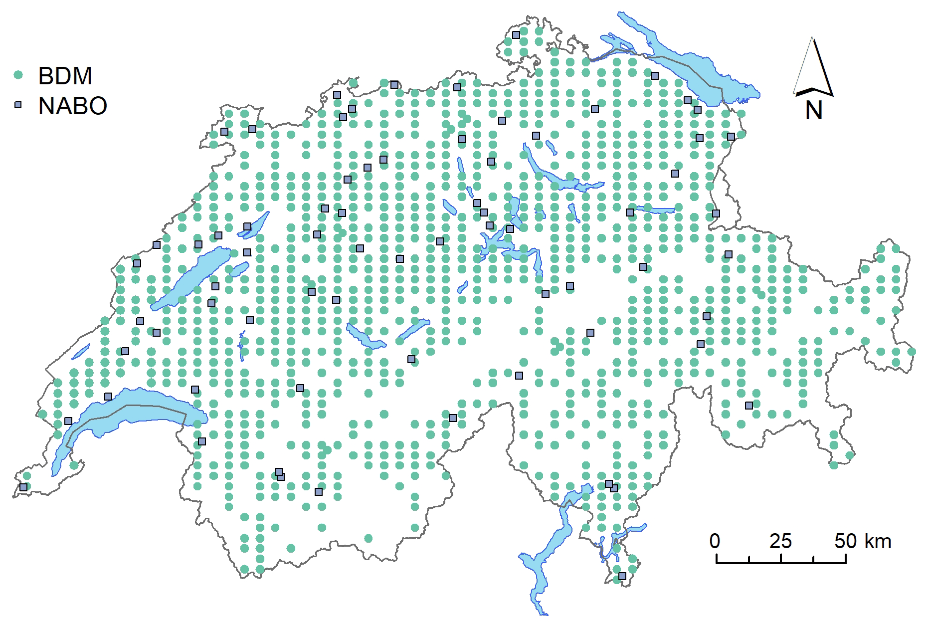
Figure 1Map of Switzerland with sampling locations of the mid-IR spectral library, including the sites of the Biodiversity Monitoring program (BDM; 6 × 4 km; n=1094) and the National Soil Monitoring Network (NABO; n=71). In total, 71 NABO sites (10 m × 10 m) were sampled with a grid-based stratified design, and 1094 BDM samples were obtained from single sampling events. The NABO sites have been continuously sampled and measured in 5-year intervals since 1985.
The plots at the NABO sites covered 10 m × 10 m each. These were repeatedly sampled for 0–20 cm soil depth. In total, four replicate samples were taken by stratified random sampling and bulking 4 × 25 cores from 100 subareas of 1 m2 to account for small-scale soil variability. Desaules et al. (2010) and Gubler et al. (2019) detailed the sample collection and data harmonization process of the measurements. The soils of the BDM were sampled at 0–0.2 m depth from positions on a regular grid of 6 km × 4 km laid over Switzerland (a total of 1094 locations). The points that were not sampled were inaccessible; these were mostly in the alpine regions. Each sampled location included four subsamples that were taken at the intersection of the four cardinal directions from the center point and the circumference of a circle with a radius of 3 to 3.5 m (Meuli et al., 2017). Due to its design which covers all major geographic regions in Switzerland – the Jura Mountains, the Central Plateau and the Alps – the BDM sampling campaign comprises a major part of the biogeochemical diversity of soils and predominant land use types in Switzerland. The wide coverage of soil conditions are an important source of soil chemical variability.
2.2 Chemical reference analysis
Data on chemical and physical soil properties were previously measured and provided by the NABO group. All laboratory soil analyses for the 16 properties were based on the protocols of the Swiss standard method (Agroscope, 1996). Mineral elements were determined by extraction with 1 : 10 ammonium acetate–EDTA solution (AAE10; method following Agroscope, 1996). The measured properties were total C, organic C (OC), total nitrogen (N), pH (CaCl2), CaCO3, clay, silt, sand, CECpot, P(AAE), K(AAE), Ca(AAE), Mg(AAE), Cu(AAE), Zn(AAE) and Fe(AAE). For samples of BDM and for the more recent NABO sampling campaigns five and six (years 2009–2014), the total C and N measurements were done with dry combustion (LECO TruSpec). For campaigns one through four (years 1985–2014), the OC contents determined with wet oxidation using a modified Walkley–Black method were transformed into dry combustion equivalents, using site-specific robust linear regressions (complementary data of campaigns five and six; Gubler et al., 2018). Carbonates were determined by volumetric calcimetry, using hydrochloric acid (HCl) for digestion. Organic C was obtained by the difference in total C and carbonate C when pH was greater than 6.5. Inorganic (carbonate) C was calculated with 0.12 × CaCO3. The texture was determined by the pipette method. The pH was measured in CaCl2, using a 1 : 2 volumetric ratio of soil to water. For CECpot, the exchangeable elements were extracted with a 0.05 N–0.025 N HCl-H2SO4 solution, which was buffered with triethanolamine for soil samples with pH > 5.9. All soil properties were referenced to dry weight by water correction after drying at 105 ∘C. All chemical analyses of NABO soils were done on four bulked replicates per site and sampling event. For BDM locations, four spatial replicates were measured each.
2.3 Measuring and processing spectra
All milled soil samples from the NABO and the BDM archive (n=4374; with a particle size below 100 µm) were measured with the VERTEX 70v Fourier transform spectrometer from Bruker (Bruker Optik GmbH, Ettlingen, Germany) at ETH Zurich, using a high-throughput accessory (HTS-XT) and custom 24-well plates tailored to diffuse reflectance measurements. The mid-IR spectrometer was equipped with a KBr beam splitter and a mercury cadmium telluride (MCT) detector, which was permanently cooled with liquid nitrogen during the measurements. The reflectance spectra were acquired between 7500 cm−1 (1333.3 nm) and 600 cm−1 (16 666.7 nm) at an effective resolution of 2 cm−1 and trimmed to the mid-IR range between 3996 and 600 cm−1 before further processing (see below).
Each soil sample was measured twice. The soil surface was flattened evenly and without compression by the thin, round middle part of the spatula. The first measurement position of the 24-well plate contained a gold (Au) reference surface, which produced a single reflectance spectrum for normalizing the reflectance of the 23 following soil measurements. The “atmospheric compensation” routine, implemented in the Bruker OPUS software, was used to eliminate unwanted absorptions of H2O vapor continuum and CO2 gas in the measurement chamber, based on the single channel reference spectrum measured once on each plate. All single channel reflectance spectra were obtained by averaging 32 internal measurements.
The resulting reflectance spectra (R; background referenced) were converted to apparent absorbance (A) by . Then, an average spectrum per sample was produced by calculating the mean of all spectral variables for the measured replicates. Finally, the spectrum offset and further scatter effects were reduced, and the features were transformed with a Savitzky–Golay (Savitzky and Golay, 1964) first derivative smoother using a window size of 35 variables (70 cm−1) and third-order polynomial fit. Finally, we selected every eighth spectral variable to reduce redundancy in the spectra (collinearity) and produce more parsimonious spectral estimates of soil properties. This resulted in 209 variables between 634 and 3962 cm−1, which formed the predictors for the subsequent general and local transfer modeling.
2.4 Data processing and statistical computing
All spectral and reference data were processed and modeled with the R software environment for statistical computing and graphics (version 3.6.0; R Core Team, 2019). We used the caret (Kuhn, 2020) R package to streamline the statistical learning process. Basic data transformations, such as data preparation and aggregation, were done using the tidyverse (Wickham, 2019) set of packages and data.table (Dowle and Srinivasan, 2019). The spectral data were handled and processed with the simplerspec (Baumann, 2019) and prospectr (Stevens and Ramirez-Lopez, 2013) packages.
2.5 General soil estimation: rules for the entire SSL
The general soil estimation was done by rules trained with the CUBIST (Quinlan, 1993) learner, separately developed for each analytical soil measure. We chose this algorithm because it has shown excellent performance for modeling soil information and developing SSLs with rather large soil variability and multicollinear spectral variables (Bui et al., 2006; Viscarra Rossel and Webster, 2012; Stevens et al., 2013; Miller et al., 2015; Peng et al., 2015; Viscarra Rossel et al., 2016; Dangal et al., 2019; Padarian et al., 2019b), and because its interpretation is mechanistically more intuitive as it is a form of data partitioning (simple conditions and linear equations). CUBIST first forms model trees, using basic mechanisms of M5 (Quinlan, 1992). CUBIST is a form of a rule-based decision tree with piecewise linear models. Wang and Witten (1996) outlined detailed principles behind the construction of the model trees and derivation of rules, and Viscarra Rossel and Webster (2012) described it for soil spectroscopic modeling.
A CUBIST prediction rule is a unique set of conditions, i.e., “if, then” logical statements, together with the associated ordinary linear regression model. During training, the condensed regression equations are made for samples in the terminal nodes. All preceding split variables are potentially allowed for regression in a final node; however, some of them are pruned or combined in the rules. The smoothed regression equations with the selected variables allows one to predict an individual, new observation. CUBIST features two empirical parameters that can improve predictions, namely committees and neighbors. Committees are ensembles of rules that are created by successive construction of trees, which correct predictions of preceding rules and, thereby, lower predictive errors by averaging. When neighbors are used (maximum nine), a new training sample is predicted, using both unweighted or weighted averages of the measured values of the nearest neighbors, using all features in the training set and the prediction of the new sample using the training rule(s).
2.5.1 Model development and validation
We tested a full-factorial combination of and100} committees of rules and and9} neighbors to tune the CUBIST models. To obtain realistic estimates of the models' general performance, we defined a grouped 10-fold cross-validation scheme that treated the entire site (e.g., for total C: NABO – 71 sites; BDM – 1079 sites) as independent in the modeling data sets. This made all observations from a site the unit of prediction, making the procedure equivalent to external cross-validation.
To reduce the bias variance trade-off in the assessment, we repeated the grouped 10-fold cross-validation (CV) procedure five times (Friedman et al., 2008; Kuhn and Johnson, 2013). The division into training and validation proportions of the data was done in consistent and repeatable manner (pseudo random number generation). We considered this site grouping factor as prior information when cross-validation segments were created, so that samples from a particular site were only present within one segment (fold) of a cross-validation split. This grouped assignment prevented the relationships from being trained on the model fitting sets and prevented a particular site from leaking into the testing segments, yielding reliable generalization errors.
We tested the correspondence of mid-IR and model-derived predictions () and measured standard reference measurements (xi) with common regression metrics. We cross-validated the inaccuracy of the models with the root mean square error (RMSE). The mean squared error (MSE) was further decomposed into mean error (ME) or bias and the standard deviation of the error (SDE) or imprecision, so that (Viscarra Rossel and McBratney, 1998). To describe the linear dependency between measurements and modeled values and give a relative goodness of fit, the coefficient of determination (R2) from linear regression was also reported. All metrics were aggregated from five estimates from independent resampling repeats. We reported mean values and standard deviations to provide uncertainties of the estimates.
2.5.2 Deriving important spectral variables
The importance of each spectral variable was assessed based on its usage in the rule conditions and the model for CUBIST. We used the recursive feature elimination (RFE) method, a backwards variable selection algorithm described by Guyon et al. (2002), to test whether the modeling can be simplified and to find most important spectral features. Soil reflectance spectra typically contain many correlated and potentially redundant variables. Therefore, constraining them to relevant subsets that feed into the modeling can further improve predictive accuracy and reduce computation time and storage for model updates. We recursively eliminated subsets of variables with low CUBIST variable importance, calculated as the average relative usage frequencies of a particular variable in split conditions and regressions. This step-wise variable reduction was based on the following predefined subset sizes Si, starting with the full set at i=1 and ending with the most important predictor at i=30:
The dropped variables at each specific reduction step received identical importance ranks, from 30 (least important variables) to 1 (most important variable). Importance ranks were determined with a step-wise variable reduction because the model-based importance of a given input variable can change substantially when some correlated variables occur more frequently than others. Otherwise, using the CUBIST importance measure on the entire spectrum would confound the importance of relevant but highly correlated variables. Since RFE is a wrapper method of variable selection, external test sets (resampling) were needed to exclude selection bias in estimating subset performance (RMSE; Kuhn and Johnson, 2013). For this purpose, we nested another inner layer of resampling for RFE within the 10-fold CV scheme repeated five times. Importance ranks of variables and outer test RMSEs were averaged from the 50 CV folds. To decrease computation time, we conducted the RFE with five CUBIST committees. The RFE procedure and the resampling setup is explained further in the Appendix.
2.6 Local soil estimation for plot-level monitoring
We defined a local soil estimation scenario where a new long-term monitoring site was initiated at time zero (t0). Each one of the 71 NABO sites was assumed to be novel, while the remaining ones were established with spectral and reference data records. We, therefore, conducted 71 separate sample selections from the SSL, each yielding different transfer subsets of the SSL, to test spectral-based soil monitoring using the Swiss mid-IR SSL presented here. We calibrated models at each site using two local samples per given site and a relevant subset of the remaining Swiss SSL (see description below).

Figure 2Conceptual scheme illustrating the transfer of the soil spectral library (SSL) to a long-term monitoring site using the RS-LOCAL approach. The local calibration samples and a subset of the SSL are used to calibrate a partial least squares regression (PLSR) model, which predicts the local validation samples.
The two local samples were chosen from pooled samples at t0 (first two out of a maximum of four replicates) or in addition at t1 if there was only one sample in t0. Figure 2 illustrates the local modeling workflow. All other samples per given site besides the two chosen during calibration (in other words, the successive time series measurements at a monitoring plot) were used as local validation samples (Nsite). The respective samples from the remaining SSL included spectra and reference measurements from all BDM samples and NABO samples, excluding the ones from the respective target site. We used only two calibration samples per NABO site to capture the predictive mechanisms at site level because we wanted to avoid overoptimistic local assessment; both local calibration and validation samples were repeated soil measurements, and are otherwise – if not adequately handled in the calibration sampling strategy – at risk of overfitting when soils' composition and relevant properties show constant trends over time.
For each of the 71 sites, the spectral relevant samples from the remaining Swiss SSL were selected using the RS-LOCAL algorithm (see Lobsey et al., 2017). The site-specific samples (msite) denote local calibration samples from a NABO plot. The recursive reductions of the initial training data, which determined the finally yielded subsets (Ksite ), were driven by model performance (RMSE) for the two local calibration samples. For each NABO site, the corresponding Ksite set was spiked with the two local calibration samples. On this combined msite+Ksite data set, a final partial least squares regression (PLSR) model, locally adapted for the monitoring plot by optimization on the calibration samples, was developed using 10-fold cross-validation. Finally, the local validation spectra (Nsite) were predicted using the most accurate calibration model.
The search algorithm RS-LOCAL has three empirical parameters to control the samples that are selected for the local transfer from the SSL (Lobsey et al., 2017). Parameter k is both the number of samples drawn from the original and reduced library without replacement and the number of samples of the returned SSL subset. Parameter b is the number of times k samples are randomly drawn from the remaining data at iteration i of the performance-driven library reduction. Parameter r is the proportion of samples, which are consistently in weakest models, that are removed at it each reduction step. The configuration of the RS-LOCAL search was optimized for each NABO site. For each site, we ran separate RS-LOCAL runs, testing a full-factorial combination of empirical parameter sets , and . The RS-LOCAL procedure is based on the PLSR (Wold et al., 1983). For the RS-LOCAL tuning during the subset selection procedure and final calibrations, we tested 1 to 10 PLSR components. The finally selected optimal subset per site yielded the smallest RMSE on the two local calibration samples and was therefore used to predict the local validation samples.
2.6.1 Uncertainty of spectral monitoring uncertainty: CUBIST vs. RS-LOCAL transfer
To compare the performance of the CUBIST approach and RS-LOCAL transfer, errors and concordance of both methods were conditionally assessed per individual NABO (n=71) site. For CUBIST, grouped cross-validation holdouts were used. Thereby, the two respective local calibration samples msite were excluded so that the test configuration was identical to the local transfer scenario. In addition to the mentioned assessment statistics, the ratio of performance to interquartile distance (Bellon-Maurel et al., 2010; RPIQ; 75th and 25th percentiles) was used for relative comparisons between the local transfer and rule-based model because it is robust to non-normal and skewed distributions of measured values.
2.6.2 Evaluating the predictive mechanisms behind the local transfer
For each of the 71 statistical transfers at a plot level, we quantified the similarity between the selected data sources Ksite (from SSL) and the respective local target domain {Nsite} (local validation) by multivariate distances across the spectral input variables. The distance of single observations within {Ksite;Nsite} was referenced to the center of all data, which led to two respective distributions of distance measures for these sets of points and per site. This procedure involved two steps, namely (1) compressing the input data to reduce the “curse of dimensionality” (Bellman, 1961) and being able to discriminate similarity with spectra (with many dimensions, distance to nearest neighbor becomes similar to distance to farthest neighbor) and (2) calculating the Mahalanobis distance using a robust method (see below; Varmuza and Filzmoser, 2016) so that the location and scatter were influenced by the main data rather than by atypical observations.
To condense the spectral information over the entire SSL, Savitzky–Golay preprocessed spectra that included all observations with C elemental measurements were mean centered, scaled and then transformed by principal component analysis (PCA) using singular value decomposition. Dimensionality reduction was necessary to avoid computationally singular values during the subsequent calculation of the covariance matrix (for the Mahalanobis distance). The first 10 principal components that explained 86.5 % of the variation in preprocessed spectra were kept for distance calculations. Finally, the Mahalanobis distance of all the observations to their center was computed with robust estimates for both the center and the covariance matrix of the selected PCA scores, using the minimum covariance determinant (MCD) estimator (Rousseeuw, 1984; Hubert and Debruyne, 2010).
3.1 Summary of reference measurements
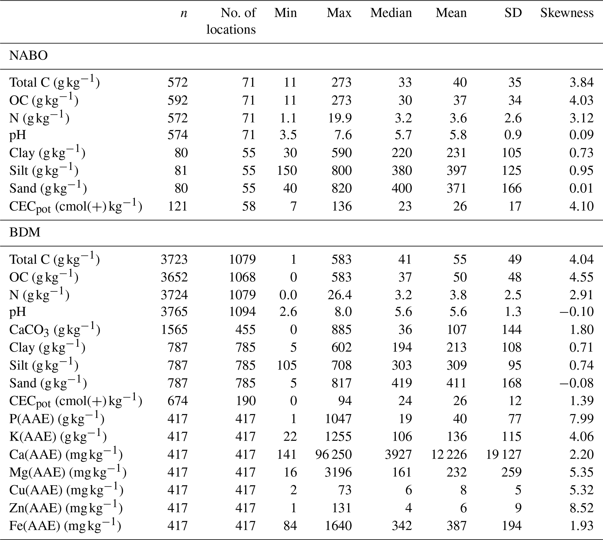
The samples from the Swiss Soil Monitoring Network (NABO) exhibited the highest variability across samples for total C and OC (n=592; Table 1). Organic C ranged from 1 to 583 g kg−1. The texture of the soils varied considerably. The pH had values between 3.5 and 7.6, and the soils were slightly acidic overall, with a median of 5.8. Compared to the NABO data set, the soils from the BDM program covered a wider set (n=3723 for total C) and range of measured soil properties. The measured range of total C for BDM (1–583 g kg−1) extended further than that of NABO. The distribution of pH values was similar in the NABO and BDM sets. The BDM data also included the available cations extracted by AAE (see Table 1). The median CECpot (potential cation exchange capacity) was almost equivalent to the value of the NABO sites (24 vs. 23 ). Exchangeable Ca showed the largest coefficient of variation (CV = 1.56) among the measured properties of the BDM set. All soil properties, except pH and CECpot, were positively or neutrally (sand) skewed for both NABO and BDM data sets, respectively.
Table 1Summary statistics of the measured soil properties of the Swiss soil spectral library derived from the sample archive of the Swiss Soil Monitoring Network (NABO) and the Swiss Biodiversity Monitoring (BDM) program. Total C is total carbon, OC is organic carbon and CECpot is potential cation exchange capacity.
3.2 General soil estimation with CUBIST modeling
For most of the properties, minimal cross-validated errors were achieved with 100 committees and nine neighbors. The rule-based models explained a large proportion of the variation (R2>0.9) in properties that typically have a strong link to total C (organic C and N; Table 2; Fig. 3). Clay was accurately estimated (RMSE = 47 g kg−1; RPIQ = 3.0; range = 0–602 g kg−1), whereas sand and silt were less accurately estimated. The pH was accurately estimated (RMSE = 0.3; RPIQ = 6.5). Our models discriminated a large proportion in the measured variation of Ca and Mg (ammonium acetate–EDTA) in the mid-IR (R2 = 0.97 and 0.79; RPIQ = 2.4 and 1.2). Reference values of potential cation exchange capacity ranged from 0 to 136 and were modeled with an RMSE of 7 (R2=0.72; RPIQ = 2.0). However, the extractable nutrients P, K, Cu and Zn were insufficiently explained by mid-IR spectral rules (R2 = 0.05–0.1; RPIQ = 0.4–0.9). Nonetheless, the rules achieved nearly unbiased property estimates over all measurements. We found marginal local bias at the largest values, mostly for variables with positively skewed distributions, such as total C (Table 2; Fig. 3).
Table 2Cross-validated mid-IR estimates of 18 soil properties derived from rule-based CUBIST models that were developed using all available data. The 10-fold cross-validation procedure was grouped by the site and repeated five times to achieve many test–train data combinations and provide a realistic model assessment with generalization. C and N denote the number of committees and neighbors for CUBIST. Total C is total carbon, OC is organic carbon, N is total nitrogen and CECpot is potential cation exchange capacity.

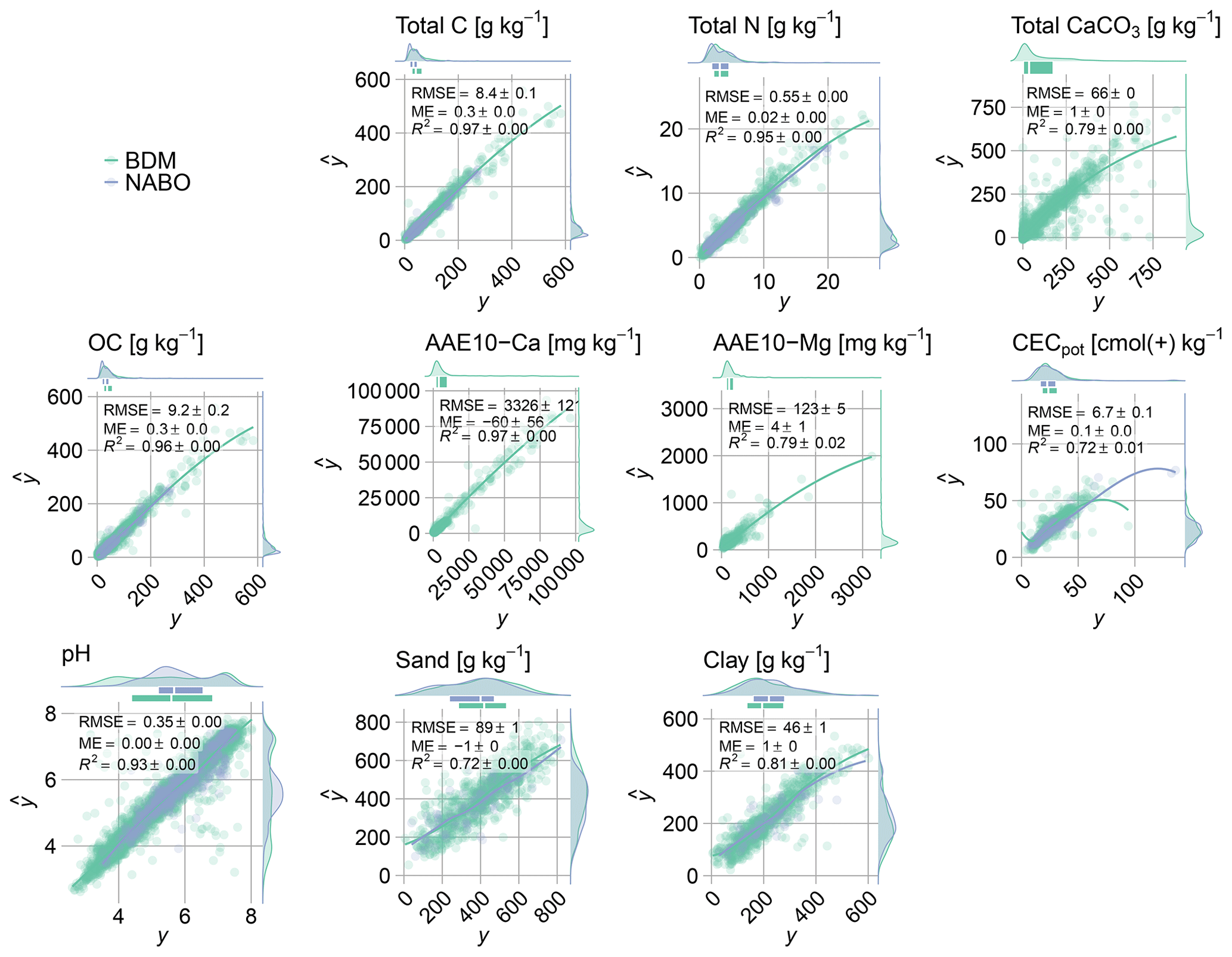
Figure 3Agreement between measured and mid-IR predicted values that were obtained from CUBIST models. Models' performance was assessed by site-grouped cross-validation holdouts (five times repeated 10-fold). The lines obtained with local regression (LOESS) smoothing indicate the trends in predictions. Models of soil properties with R2≥0.72 are shown (see Table 2 for more detailed model summaries).
Overall, out of the 16 available soil properties, total C, total N, total CaCO3, Ca and Mg (ammonium acetate–EDTA), OC, CECpot, pH, sand and clay (10) were modeled with relatively good discrimination capacity in the measured ranges (Fig. 3).
Model interpretation and filtering with variable importance
Figure 4 shows that the test RMSE of total C first slightly decreased and then steadily increased from all (209) to less spectral variables using CUBIST and RFE. The lowest error (RMSEtest = 8.10 g kg−1 total C) of spectroscopic estimation was achieved with the spectra with 105 variables. For the subsequent variable reduction steps, model performance steadily dropped until one wavenumber was left (RMSEtest = 18.8 g kg−1 total C).

Figure 4(a) Root mean square error (RMSE) of mid-IR estimates of total C that CUBIST produced at the respective subsets of spectral variables. The performance profile was obtained with a recursive feature elimination (RFE) procedure. The error bars represent the standard deviations of the test RMSE derived with nested cross-validation (n=50). (b) Average importance ranks across the spectrum. Lower rank values indicate higher importance for the estimation of total C. Ranks were determined with RFE. (c) Mid-IR absorbance spectra of the Swiss soil spectral library (n=4295; with corresponding total carbon (C) measurements determined by dry combustion). The unprocessed absorbance spectra are annotated with the 17 most influential spectral variables (wavenumbers) in the CUBIST model (average importance rank <15); these had the highest mean importance ranking determined by the recursive feature elimination procedure.
The spectral feature between 1786 and 1754 cm−1 was the most important one for the estimation of total C with CUBIST (Fig. 4). The 12 spectral variables with the best importance ranks across all RFE iterations and test sets derived from the subset sizes were (starting with the best) 1754 (mean(rank)=1.04), 1786, 1770, 2010, 2506, 1850, 1370, 2522, 1818, 1866, 2058 and 1386 cm−1 (mean(rank)=12.7; Fig. 4).
3.3 Accuracy of the local transfer models compared to the general model
For the example site 65 COR, the best performance of RS-LOCAL was achieved with 55 samples from the SSL (K), 10 sampling events (B) of size K at each iteration and 10 % reduction (r) at each iteration (Fig. 5). Therefore, 55 transfer samples from the SSL were combined with two site calibration samples previously used to supervise the selection from the data source, to form a PLSR calibration model for the estimation of the site validation samples (see Fig. 5a; right). Compared to the target observations from the site (right part of Fig. 5a and b; measured range = 11.9–16.0 g kg−1 C), the selected instances were heterogeneous with regard to their characteristic patterns in raw spectra, their preprocessed feature space and their measurements (range = 8.7–97.7 g kg−1 C). The selected instances covered a significant proportion of the first two components in the feature space of the entire SSL.
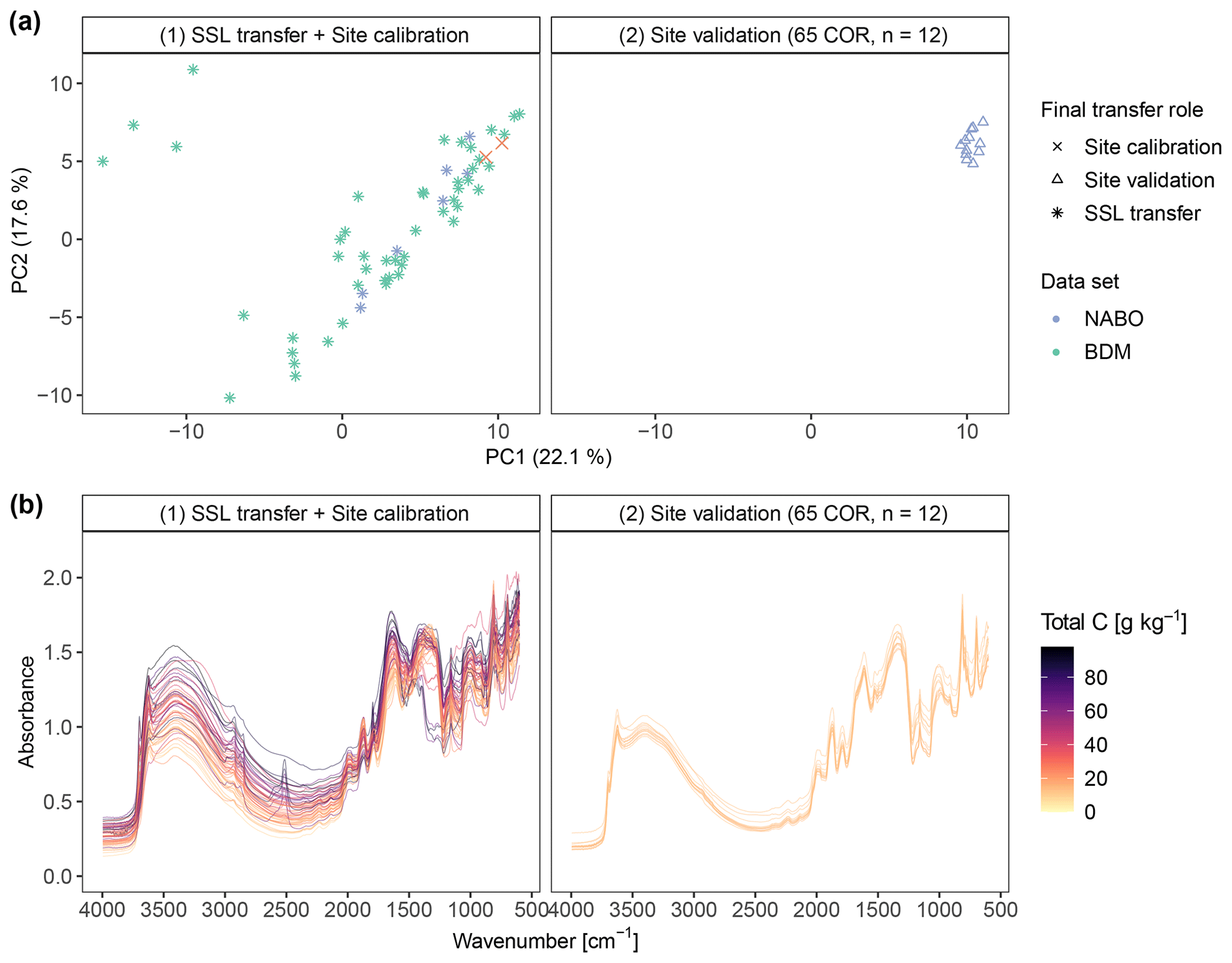
Figure 5Illustration of the site-specific transfer modeling of total carbon (C) using RS-LOCAL for the example site 65 COR of the Swiss Soil Monitoring Network (NABO). Panel (a) contains the principal components subspace (PC1 and PC2) of the Savitzky–Golay first derivative mid-IR spectra, and panel (b) outlines the corresponding absorbance spectra (unprocessed for illustration), which are colored by the total C content. The left subplots show the SSL transfer samples (n=55) that were selected from the soil spectral library (n = 4281; excluding all NABO calibration samples). This subset was most accurate when predicting the two calibration samples under the mechanisms RS-LOCAL and their optimal tuning configuration for the site (). The right panels shows the time series data for the validation samples of the NABO site called 65 COR.
The RMSE on the site validation samples () at the final subsets varied between 0.01 and 10.73 g kg−1 C and for all tuning parameter combinations and sites and between 0.01 and 3.02 g kg−1 C for the best subsets per site (Fig. A1).
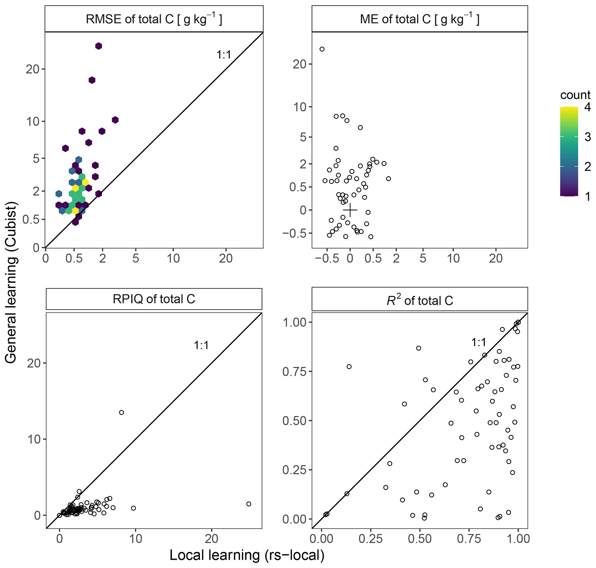
Figure 6Model assessment of the estimated total carbon (C) of 71 NABO sites for the general learning with CUBIST (y axis) vs. local learning transfer with RS-LOCAL (x axis). The four panels depict the root mean square error (RMSE), the mean error (ME), the ratio of performance to interquartile distance (RPIQ) and R2. The 1 : 1-line emphasizes the difference between the two approaches.
The local approach reduced the error of the rule-based approach on average by factor 4.4 (Fig. 6; mean(RMSERS-LOCAL) = 0.7 g kg−1 C; mean(RMSECUBIST) = 3.1 g kg−1 C). The local transfer was more accurate for the majority of NABO sites (69 out of 71 sites). The linear dependency between modeled and measured values was higher for the local transfer compared to the general model (53 out of 71 sites). Moreover, RS-LOCAL produced on average 1.3 times less biased estimates of total C per site for 52 out of 69 sites in terms of absolute values ( = 0.1 g kg−1 C vs. 0.5 g kg−1 C). The ratio of performance to interquartile distance (RPIQ) confirmed that local learning in the mid-IR was able to better discriminate developments of total C over time, relative to its measured distribution. Overall, local learning with two local calibration samples and targeted SSL selections allowed for better estimations than the generic CUBIST approach on average (RPIQ = 3.08 vs. 1.00; RPIQ larger for 66 out of 71 sites). Across all validation data points of the NABO set, the RS-LOCAL transfer was 5.6 times more accurate for total C than the general rules in terms of RMSE and RPIQ (RMSE = 0.9g kg−1 C; RPIQ = 31.7)
Predictive mechanisms behind the local transfer
The samples used for the transfer process (RS-LOCAL data) of the example site COR 65 showed high spectral dissimilarity along the first 2 PCs (principal components), explaining 39.8 % of the preprocessed spectral variance (Fig. 5). Compared to the entire SSL with total C measurements available (the source domain prior selection; range of PC1 from −41.4 to 13.0; range of PC2 from −19.0 to 30.0), the selected transfer samples of this site occupied a region of major variation in the PC space (range of PC1 from −15.4 to 11.4; range of PC2 from −10.2 to 10.9). The two local calibration samples and the 12 validation samples in the upper right corner were close to each other in the PC1–PC2 subspace (Fig. 5a; left and right; range of PC1 from 9.2 to 11.0; range of PC2 from 4.9 to 7.5). Not only the absorbance spectra but also the corresponding C reference values were highly variable compared to the exemplary NABO site (Fig. 5b; 7.3–117.8 g kg−1 C for KRS-LOCAL and 11.9–16.0 g kg−1 C for the plot of this site). This particular target monitoring site indicated that RS-LOCAL selected soils from the SSL with a relatively large spectral diversity and a wide range of total C.
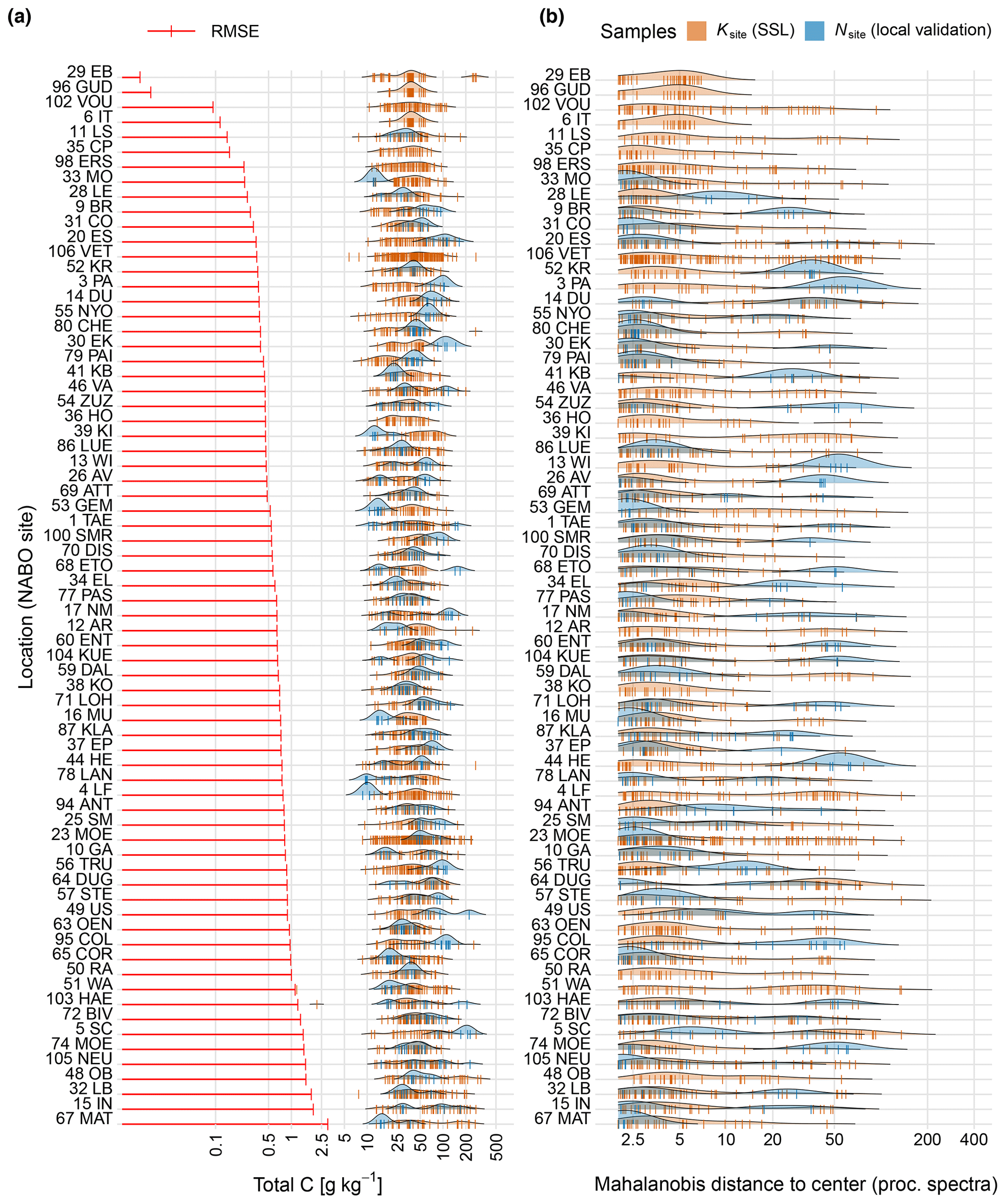
Figure 7Analyzing the mechanisms behind the individual adaptive transfer realized with RS-LOCAL. (a) The left horizontal bars show the root mean square error (RMSE) of mid-IR predictions of the temporal validation set Nsite of time series of total carbon (C) for each of the 71 NABO sites, which was calculated without the two respective calibration samples. The blue density plots depict the distribution of the site-specific validation samples, and the brown vertical bars show the measured values of C for the final subsets of SSL used for the transfer (Ksite). (b) The distribution of the robust distances from the PCA center of the Savitzky–Golay preprocessed spectra of the entire soil spectral library compared to the subset of instances involved in the individual transfer modeling (Ksite) and validation samples (Nsite; similarity in site-specific vs. final RS-LOCAL selection) computed with the minimum covariance determinant (MCD) estimator.
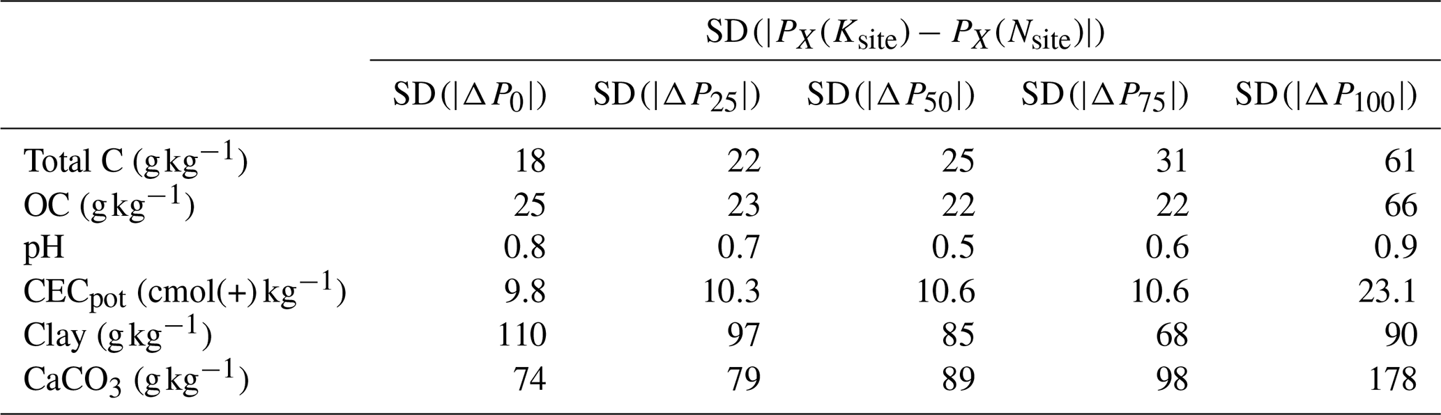
The instances selected by RS-LOCAL filled a substantial proportion of the SSL's feature space (Fig. 7), confirming the trend of site 65 COR. We found that RS-LOCAL yielded quite a wide selection of relevant samples from the SSL with reference to both the total C range and a wide coverage of spectral features expressed with robust multivariate locations. The spectral estimations of the site validation sets that resulted from RS-LOCAL-based transfers neither showed trends in the mode or spread for distributions of C measurements nor in the ones from their spectral distances. The measured distributions of Ksite SSL subsets and Nsite local validation samples for further key soil properties related to the chemical composition (OC, pH, CECpot, clay and CaCO3) were also markedly different, confirming the local transfer of quite heterogeneous soils (Table 3). For example, standard deviations of the 0 %, 25 %, 50 % and 75 % percentile differences between the transfer sets selected the SSL and the samples from the respective NABO site were on average between 18 and 66 g kg−1 for measured C and OC, respectively. Furthermore, the measured clay and CaCO3 contents were markedly different between the RS-LOCAL selection and the local validation sets (mean absolute median differences of 85 g kg−1 clay and 89 g kg−1 CaCO3). These findings correspond with the dissimilar selection compared to the local target samples found in the PCA space of preprocessed spectra.
Table 3Standard deviations (SDs) of the absolute differences in percentiles ( and P100) of final RS-LOCAL subsets (Ksite) and corresponding site validation samples (Nsite) the across 71 long-term monitoring sites. The aggregated values for six measured soil properties are shown. Total C is total carbon, OC is organic carbon and CECpot is potential cation exchange capacity.
4.1 General soil estimation with the Swiss SSL
Many of the chemical properties with distinct links to soil organic matter and the key minerals (e.g., clays and quartz) were discriminated well with mid-IR CUBIST models (Table 2; Fig. 3). Specifically, the models estimated total C, OC, N, pH, texture, AAE10-Ca and AAE10-Mg with R2>0.7. This suggests that the majority of developed models are useful for applications that require soil proxies in order to manage land resources. For example, CECpot (RMSE = 7.0 ) and pH (RMSE = 0.3) have high ecological importance for nutrient availability in ecosystems. In agriculture, both measures are key factors for soil fertility and nutrient recommendations.
The accuracy of our estimates for the properties that have direct chemical links, through compound-associated absorptions, were mostly comparable to established continental or country-specific mid-IR SSLs. For example, Clairotte et al. (2016) achieved RMSE=2 g kg−1 for OC using mid-IR and the spectrum-based learner for local predictions, while Sila et al. (2016) reported RMSE=4 g kg−1. The accuracy of our general OC estimates was lower (RMSE=9.3 g kg−1; RPIQ = 3.4), which we explain with the relatively large range of measured values and variable mineralogy (Stenberg and Rossel, 2010). We found that total C had more CUBIST rules per committee than OC (Table 2), indicating that total C, which also included inorganic C (mostly CaCO3), leverages more chemical constituents and latent absorptions for its estimation. In spite of lower parsimony, slightly more accurate estimates of total C were achieved (RMSE=8.4 g kg−1; RPIQ = 4.3).
The majority of soil properties were most accurately estimated with the maximum tested 100 committees and nine neighbors. Instance-based correction with similar data in the training set, (nearest) neighbors, yielded considerably higher accuracy for total C (e.g., RMSE = 8.9 g kg−1 for 20 committees and two neighbors vs. RMSE = 8.1 g kg−1 for 20 committees and nine neighbors; model evaluation across cross-validation folds; results not shown). The number of rules give a first proxy for model complexity and the complementary of spectral features that are involved in prediction. The range in number of rules across the ensembles was widest for total C (6–26), similar for OC (4–24), medium wide for CECpot (1–10) and very narrow for CaCO3 (1–5), to give specific examples. Viscarra Rossel and Webster (2012) report comparably fewer rules (medium – 21; range of all properties – 5–64) for OC and relatively similar number of rules for CEC (15). Nonetheless, such comparisons have to be done with care because the NIR range has a less pronounced representation of functional groups than the mid-IR range and because temperate soils have fundamental differences in chemical composition compared to more weathered tropical soils. For our mid-IR SSL, we were surprised that the rules for OC were complex, similar to the ones for total C; in fact, we also could not find any clear partitioning in the rules with respect to measured ranges and spectral patterns (exploratory analysis not shown), which is in contrast to Viscarra Rossel and Webster (2012). In fact, this is different from the general patterns found by Viscarra Rossel and Webster (2012), where the rules clearly partitioned the data into distinct measured distributions. Last but not least, the diversity in rules for total C and OC of the general estimation approach makes the soil diversity selected from the library and what we found for site-specific local transfer even less exotic (see Sect. 4.2).
The variable importance assessment of the spectroscopic models revealed five major regions of features with particularly high predictive influence for total C, i.e., 2890, 2522, 2010, 1754 and 1370 cm−1 (Fig. 4). We attribute the two absorption peaks near 2890 cm−1 to C−H stretching vibrations of organic matter (Skjemstad and Dalal, 1987), which were also relatively important for estimating C in other studies (e.g., Janik and Skjemstad, 1995; Viscarra Rossel and McBratney, 1998). The important variable at 2522 cm−1 is indicative of C=O absorption due to the carbonyl group present in carbonates (e.g., calcite; Nguyen et al., 1991; Soriano-Disla et al., 2014). The three important absorptions between 2010 and 1786 cm−1 result from three consecutive (overtone and combination) absorptions, which are indicative of quartz. However, the most important absorptions near 1754 cm−1 showed no distinct peak but an edge feature. This is in accordance with Sila et al. (2016), who identified this region as being most relevant for estimating total C with a (general) random forest model developed from the SSL of the Africa Soil Information Service. This region is close to the C=O stretching vibration of the carboxyl group that occurs around 1725–1720 cm−1 (Madari et al., 2006), which is further confirmed by the high importance of these vibrations found by Janik and Skjemstad (1995). The last relatively important region around 1370 cm−1 was also an edge feature with no distinctly visible peak of chemical group assigned, which, however, might be influenced by the adjacent carboxylate (COO−) or −CH absorptions at 1400–1350cm−1 of aliphatic compounds such as humic acids (Madari et al., 2006; Parikh et al., 2014). In summary, the CUBIST–RFE variable importance analysis enabled us to link characteristic absorptions of typically prominent functional groups of soil organic and inorganic C compounds, as well quartz absorptions as indirect correlative features of predictive relevance, with our general model-based estimates of total C.
Because the rule-based models we developed can estimate 10 soil properties reasonably well (R>0.6; RPIQ >2.0; Fig. 3), the Swiss SSL will be useful for new soils when new reference measurements for model adaptation are relatively scarce or not available. Thereby, the Swiss SSL will be cost and time efficient for characterizing soils of similar composition in the near future. The new predictions can further be augmented with straightforward model interpretation, which allows the chemical inference of pedological aspects to provide means of model applicability. Although the combined BDM and NABO set comprises a large soil variability in Switzerland, the diversity of subsoils at depths greater than 20 cm – mostly in terms of the mineral composition – and peat and forest soils are probably not yet represented sufficiently in the SSL. We must therefore continuously update the present SSL with more and deeper soil horizons in the near future.
4.2 Local transfer from the SSL for soil monitoring at plot scale
The local estimates of total C that were derived with RS-LOCAL selection were substantially better on average (RMSE = 0.7 g kg−1 C) than those derived using all of the data and general CUBIST models (RMSE = 3.1 g kg−1 C; Fig. 6). The data-driven estimation at plot scale further considerably reduced bias and increased R2 compared to the general CUBIST rules.
Our third goal was to analyze the characteristics of soils that were selected from the SSL and used for establishing locally adaptive models tailored to the respective long-term monitoring sites. Surprisingly, the RS-LOCAL subsets selected from the SSL had rather dissimilar spectra in the robust PCA space (Figs. 5 and 7); their distances to the center had a wide distribution compared to the local samples. The Ksite subsets accordingly covered a large proportion of the spectral input space. The likely dissimilar chemical composition of soils was also reflected in the reference measurements of total C. We conducted a broader analysis to interpret the soil context of the selected samples with further soil compositional covariates (OC, pH, CECpot, clay and CaCO3), which also did not resemble the soil characteristics of the local monitoring sites (see Fig. 3). These findings, together with the accurate validation results, clearly indicate that dissimilarity and diversity in soils can also provide the means for fitting locally adaptive models.
Nevertheless, we can yet only speculate about how and why such diverse calibration sets are able to leverage accurate local calibrations. One hypothesis is that, by increasing the range of and variability in spectral variables and measurements, a model can become quite stable in the central range of local reference measurements because a larger range of input variables is considered; thereby, the RS-LOCAL subsets that are selected from the SSL and used for PLSR would stabilize and reduce the errors of the local samples. We imagine that we leverage a similar mechanism as in simple linear regression, where narrowing the range of the independent variable (x) in the training samples would decrease the accuracy of intermediate values of the independent variable. We therefore need to look further into the details of spectral dissimilar learning and, for example, also investigate the relevance of specific spectral features for local spectral transfers. The inherent working principles of RS-LOCAL are in contrast to the spectrum-based learner (SBL) or other forms of memory-based learning that utilize similar samples to infer sample-specific predictions based on existing training data (Lin and Vitter, 1994; Ramirez-Lopez et al., 2013). Our approach could describe a data-driven phenomenon, which implies that spectra can help to estimate a set of unrelated new soils. Another possibility is that there is in fact a pedological explanation that could be elucidated with more soil covariates, such as mineralogy.
Local soil characterization is simpler, quicker and cheaper when a large proportion of properties of new soils are estimated by spectroscopy. Our results suggest the importance of optimizing the transfer of relevant information present in large SSLs to minimize the required amount of conventional laboratory analyses of new soils. Soil chemical and physical heterogeneity can be substantial in large SSLs. Therefore, such data variation can be beneficial for future predictions of the properties of soils. However, the machine learning of a single general model over a heterogeneous training set, and obtaining parameter estimates optimized with a global measure of goodness of fit, can introduce bias and inaccuracy to local (soil) estimation (Hand and Vinciotti, 2003; Ramirez-Lopez et al., 2013; Lobsey et al., 2017). Although the highest estimation accuracy could be achieved only with soils of the target study area (Stenberg and Rossel, 2010; Guerrero et al., 2016), it is impractical and inefficient to derive a single spectral prediction model with those. It requires (1) a large volume of reference measurements for a reasonably accurate multivariate calibration, and (2) it does not utilize already existing soil information.
Currently, the Swiss long-term soil monitoring uses a spatially representative sampling and then bulks the soils into four replicates for reference measurements (Desaules et al., 2010; Gubler et al., 2019). When the long-term monitoring would be augmented with mid-IR spectroscopy, one could make spectral measurements on all subsamples, rather than only on bulked samples, which would deliver spatially explicit information and reduce nuisance factors from different sampling conditions. If not constrained economically (separate drying, sieving and milling of subsamples), a spectral workflow could thus allow one to account for small-scale soil variability and reduce bias in measurements to robustly estimate temporal soil changes. For example, there is currently a relatively large variability in C measurements between the bulked replicate samples at one point in time (Gubler et al., 2019). Our results suggest that unbiased spectral measurements eventually mediate such inconsistencies. Although Gubler et al. (2019) reported only minor changes for the ensemble of permanent cropland or cropland–meadow monitoring sites (30), there were four sites with declining trends and nine sites with increasing trends in OC (−11 % to +16 % relative change per decade, respectively). Here, the trend of spectroscopic predictions could be investigated with respect to specific research questions on agronomic management-induced changes, also with further physicochemical soil characterization (e.g., OC fractions).
Relatively precise and unbiased geographically local estimates of soil properties from diverse and large SSLs can be achieved by a handful of data-driven statistical approaches that are currently popular in the soil science community (Viscarra Rossel and Webster, 2012; Ramirez-Lopez et al., 2013; Guerrero et al., 2014; Lobsey et al., 2017; Tsakiridis et al., 2020). Among the methods, we tested RS-LOCAL Lobsey et al. (2017) in our local soil monitoring scenario. Compared to memory-based learning, such as SBL (Ramirez-Lopez et al., 2013), RS-LOCAL does not precondition the choice of useful subsets based on similarity in the input dimensions, here spectra, when performing the selection of SSL samples. The RS-LOCAL method is applied to exhaustively sample instances from the SSL without replacement, while it preferably selects those that perform well on the local target set, using PLSR. An advantage of the method is that it can deal better with erroneous spectra, and inaccurate and imprecise analytical reference measurements in the SSL, because it filters them as irrelevant instances. Besides chemometric and classical machine learning approaches, convolutional neural networks are being popularized for modeling SSLs with large soil variability (e.g., Liu et al., 2018; Padarian et al., 2019a, b; Tsakiridis et al., 2020). There seems to be a small performance gain of a multi-output CNN with a similarity-based error correction using neighbors compared to the SBL (Tsakiridis et al., 2020; RMSE = 11 g kg−1 vs. 12 g kg−1 for OC). Despite the current development of interpretation methods in deep learning, CUBIST and PLSR modeling employed in both in the SBL and RS-LOCAL offer easier interpretation with comparable accuracy to CNNs.
Transfer learning or local learning introduces a new paradigm to supervised learning, i.e., model building that is governed by the intended model application and thus coupled to it (Hand and Vinciotti, 2003). This contrasts with the general model application, where the inference process is separated from the prediction of new data. Including local samples and their local data characteristics is necessary so that a combined search and learning algorithm has a chance to capture predictive mechanisms. At the same time, the selection process and the partial data dependence within the predictive unit, the site, requires a careful assessment scheme to prevent a potential selection bias in the assessment of the approach. To account for this, we kept the respective site-specific local tuning and calibration set – whose holdout performance directed the iterative search process and the reduction of the SSL – at minimum size of two observations at t0 or, in addition, t1 when only one measurement was available from the first sampling (see Fig. 2).
4.3 Future applications and updates of the SSL
We found that data-driven modeling with a selection of spectrally dissimilar soils (see Fig. 7) is accurate for inducing local predictions of total C (Fig. 6). Hence, there is the need to further improve the data-driven selection using RS-LOCAL, i.e., by further optimizing the current version of the algorithm. To address this need, we could use combined memory-based or lazy learning strategies (Stanfill and Waltz, 1986; Lin and Vitter, 1994; Ramirez-Lopez et al., 2013) to optimize with more data-driven transfer methods (Pan and Yang, 2010) in terms of reducing the time needed to evaluate suitable subsets of the SSL for a new application. To give an example, some similarity criteria or clustering before doing calibration sampling could be used as prior information for reducing the SSL size to obtain the final subsets. In principle, the sample reduction could also be done with algorithms that can deal with nonlinear relationships between spectra and soil properties, such as random forest or CUBIST. Another extension is to further filter spectral features and to do data compression to make the local modeling faster and even more adaptive to local conditions.
Our results showed that a transfer of the SSL to individual monitoring sites yielded very low bias and was accurate. This indicates that mid-IR spectroscopy and SSLs have the potential to give quick and relatively precise soil property estimates for soil monitoring. Nevertheless, the sites of the NABO long-term monitoring program has not undergone substantial changes in OC (Gubler et al., 2019). Up to now, although major changes in C content and organic composition should yield a spectral response, spectral changes in OC have mostly been reported along chronosequences (i.e., Awiti et al., 2008) and only rarely for changes within individual plots over time (Deng et al., 2013). Hence, to address this, we propose to further investigate to what extent mid-IR spectroscopy can detect changes of OC, considering small-scale variability and different agronomic management practices. This could, for example, be achieved with a study using soils from a long-term field trial that shows sufficient temporal changes to be detected with spectroscopy.
The current SSL includes soils that contain between 0 and 583 g kg−1 total C and OC (Table 1). Because organic soils can have up to 500 g kg−1 OC, and because more than 98 % of the samples are mineral soils, organic soils are underrepresented in the current Swiss SSL. For this reason, Helfenstein et al. (2021) evaluated the present Swiss SSL for a regional transfer based on new organo–mineral soils from two peatland regions in Switzerland. Although the range of total C measured was large (14–520 g kg−1 C) and the soils were diverse, as few as 5 or 10 site-specific tuning samples were sufficient to estimate the validation samples with reasonable accuracy (RMSE = <30 g kg−1 C; RPIQ >3.4); this was comparable to a local-only calibration with 50 samples. Helfenstein et al. (2021) found considerably lower conditional prediction errors (<10 g kg−1) when considering measurements of <100 g kg−1; this suggests that increasing the amount and compositional complexity of organic soils in the library has potential for more accurately characterizing diverse soil ecoregions with soils that have high organic matter contents.
Our results suggest that the present mid-IR SSL has great potential for applications that require soil data in high temporal and spatial coverage (i.e., for deriving quantitative indicators of soil quality for spatial planning or for soil-related environmental research). Mid-IR spectral modeling was able to estimate many soil properties accurately with a rather large variation in measurements being explained (Fig. 3), making them suitable for agronomic diagnosis and the assessment of soil functions in various landscapes. Currently, fine-grained soil information on the properties and functions across agricultural lands in Switzerland is still scarce and often challenging to harmonize (i.e., measurement methods) because legacy maps are at varying levels of detail and quality (Keller et al., 2018; Grêt-Regamey et al., 2018). For example, only 13 % (127 000 ha) of soil in agricultural land has been mapped with soil attributes of sufficient quality to evaluate its potential for crop production (Rehbein et al., 2020). Soil properties are also insufficiently mapped nationwide from points into space, depth and over time to regionally model soil processes or to evaluate site-specific effects of agricultural practices on soils (i.e., soil C dynamics). Therefore, we suggest coupling infrared spectral estimations with traditional soil surveys and digital soil mapping to speed up the collection of soil information in Switzerland and elsewhere. This will offer the means to test and further extend this SSL so that only minimal amounts of costly and time-consuming traditional laboratory analyses will be needed for characterizing and mapping soils' properties and functions in the next decades.
We developed the Swiss mid-IR SSL (n=4374), using legacy soils and reference measurements of 16 properties, from 71 long-term monitoring sites (National Soil Monitoring Network; NABO) and 1094 locations sampled from a regular grid over Switzerland (Biodiversity Monitoring program; BDM). The trained CUBIST models – a general modeling approach using all data – were able to explain a relatively large proportion (R2≥0.72; RPIQ ≥ 2.0) of measured variance for 10 of the properties. Total C, OC, total N, pH, CECpot and clay content were estimated with high discrimination capacity (R2>0.8; RPIQ >3.0). Total C was estimated with a cross-validated RMSE = 8.4 g kg−1 at a measured range of 0–583 g kg−1 and OC with RMSE = 9.3 g kg−1 at the same measured range. Compared to the general CUBIST approach, the local transfer yielded on average 4.4 times more accurate estimates of total C with the mean RMSE = 0.7 g kg−1 C, which is a substantial improvement on local estimates at plot scale. Our similarity analysis revealed that local learning with subset selection based on RS-LOCAL produced a chemically diverse calibration set rather than narrowing down soil diversity for local modeling, as it is, for example, the case in memory-based learning. The developed national mid-IR SSL offers rapid soil estimates which are key inputs for many applications requiring soil information, such as digital soil mapping, agronomic diagnostics and precision farming, soil C accounting and monitoring, etc. The created mid-IR SSL and both local and general models can be updated with new soil records, which will us allow to cover more soils conditions and will require fewer and fewer soil laboratory reference measurements in relation to spectral measurements for monitoring, mapping and modeling new soils.
A1 Recursive feature elimination for interpreting general soil estimation with CUBIST
The recursive feature elimination (RFE) procedure started with the initial set of S1=209 predictive variables that resulted after processing the spectra (see Sect. 2.3). The following subset sizes Si representing the number of spectral variables that are retained after each ith variable elimination step were defined and evaluated within the RFE procedure:
The first variable elimination step (i = 1) started with tuning a full CUBIST model derived from S1=209 possible predictors using 10-fold cross-validation, calculating the CUBIST model usage statistics for all predictors, sorting all predictors from highest to lowest importance and, lastly, dropping of the least important predictors. For the next iteration (i=2) and the following ones, we repeated this model fitting and variable reduction procedure with S2=150 predictors and the preceding subsets until the most important predictive variable (S30=1) was left at the last iteration (i=30).
Variable selection is, in addition, prone to overoptimistic model assessment when resampling subsets (i.e., cross-validation) are used for two purposes, namely model building and selection. This selection bias due to data leakage is well documented for so-called wrapper methods of variable selection, like RFE (Ambroise and McLachlan, 2002; Kuhn and Johnson, 2013), and occurs if these two tasks are not sufficiently separated by using independent data sets for each of them; this becomes especially more important when many predictive variables in relation to relatively few observations are used, as it the case for our spectra.
To provide realistic predictive generalization of the RFE method, the aforementioned iterative selection procedure was done within an internal cross-validation scheme so that independent data were used to test the performance of the variable selection on the outer data segments. These outer cross-validation segments served external validation. To quantify the uncertainty of the models using the reduced variable sets and, specifically, variable selection, the outer cross-validation layer that served as cross-validation was repeated five times, leading to five independent estimations per sample.
A2 Tuning profile of the RS-LOCAL parameters for local predictive transfers
The most relevant samples from the SSL at each respective NABO long-term monitoring plot were empirically selected at the RS-LOCAL configuration that yielded the lowest RMSE on two calibration samples per plot (Fig. A1; performance profile). The time series validation on the remaining samples of each site was separated from the optimization in the transfer workflow (see Fig. 2).
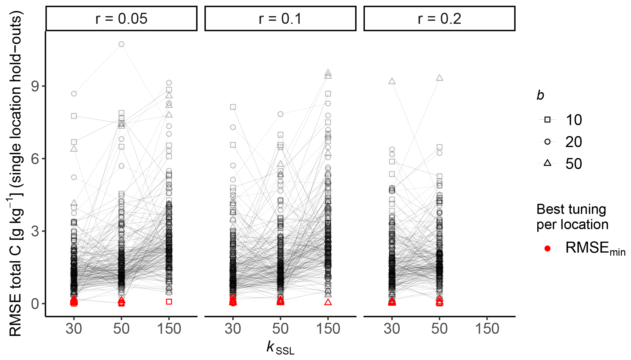
Figure A1Performance profile of the 27 empirical parameter combinations of RS-LOCAL tested on each of the 71 NABO sites. The root mean squared error (RMSE) of the plot-level transfer was assessed with the first two calibration samples for each time series of total carbon (C; see Fig. 1 for an illustration of the setup of the local predictive transfer).
The data that were used to produce the results of this paper are available upon reasonable request.
PB prepared the draft, conceptualized the spectral modeling scenario, carried out the data analysis and wrote the code. JL and JS developed the concept of a Swiss Spectral Library. All co-authors contributed to writing the paper. DW and RGM contributed to writing the methods section, AH contributed to the introduction, results and the discussion, and AK provided inputs to writing the introduction and the conclusion. AG created the map of locations and contributed to writing the methods and the discussion. RVR helped guide the spectral modeling experiments and provided the implementation of RS-LOCAL in R.
The authors declare that they have no conflict of interest.
Publisher’s note: Copernicus Publications remains neutral with regard to jurisdictional claims in published maps and institutional affiliations.
We express our thanks to Leonardo Ramirez-Lopez, Laura Summerauer and Jonas Anderegg, for their valuable inputs that helped to improve the paper. This research was funded by ETH grants. We also would like to express our gratitude to the Federal Office of Environment for commissioning and funding the soil analyses conducted within the BDM. NABO provided the milled soil archive of NABO and BDM, together with the chemical reference data and metadata.
This research has been supported by ETH Zurich (ETH-40 Grant; grant no. 1-001269-000).
This paper was edited by Bas van Wesemael and reviewed by two anonymous referees.
Agroscope: Schweizerische Referenzmethoden der Forschungsanstalten Agroscope, avaiable at: https://www.agroscope.admin.ch/agroscope/de/home/themen/umwelt-ressourcen/monitoring-analytik/referenzmethoden/standortcharakterisierung.html (last access: 16 August 2021), 1996. a, b
Ambroise, C. and McLachlan, G. J.: Selection Bias in Gene Extraction on the Basis of Microarray Gene-Expression Data, P. Natl. Acad. Sci. USA, 99, 6562–6566, https://doi.org/10.1073/pnas.102102699, 2002. a
Angelopoulou, T., Balafoutis, A., Zalidis, G., and Bochtis, D.: From Laboratory to Proximal Sensing Spectroscopy for Soil Organic Carbon Estimation – A Review, Sustainability, 12, 443, https://doi.org/10.3390/su12020443, 2020. a
Awiti, A. O., Walsh, M. G., Shepherd, K. D., and Kinyamario, J.: Soil condition classification using infrared spectroscopy: A proposition for assessment of soil condition along a tropical forest-cropland chronosequence, Geoderma, 143, 73–84, https://doi.org/10.1016/j.geoderma.2007.08.021, 2008. a
Baumann, P.: philipp-baumann/simplerspec: Beta release simplerspec 0.1.0 for zenodo, Zenodo [code], https://doi.org/10.5281/zenodo.3303637, 2019. a
Bellman, R.: Adaptive Control Processes: A Guided Tour, Princeton University Press, available at: http://www.jstor.org/stable/j.ctt183ph6v (last access: 16 August 2021), 1961. a
Bellon-Maurel, V., Fernandez-Ahumada, E., Palagos, B., Roger, J.-M., and McBratney, A.: Critical review of chemometric indicators commonly used for assessing the quality of the prediction of soil attributes by NIR spectroscopy, TrAC-Trend. Anal. Chem., 29, 1073–1081, https://doi.org/10.1016/j.trac.2010.05.006, 2010. a
Briedis, C., Baldock, J., de Moraes Sá, J. C., dos Santos, J. B., and Milori, D. M. B. P.: Strategies to Improve the Prediction of Bulk Soil and Fraction Organic Carbon in Brazilian Samples by Using an Australian National Mid-Infrared Spectral Library, Geoderma, 373, 114401, https://doi.org/10.1016/j.geoderma.2020.114401, 2020. a
Bui, E. N., Henderson, B. L., and Viergever, K.: Knowledge Discovery from Models of Soil Properties Developed through Data Mining, Ecol. Model., 191, 431–446, https://doi.org/10.1016/j.ecolmodel.2005.05.021, 2006. a
Bundesamt für Umwelt (BAFU): Biodiversitätsmonitoring Schweiz BDM, Koordinationsstelle BDM 2014: Biodiversitätsmonitoring Schweiz BDM. Beschreibung der Methoden und Indikatoren, Umwelt-Wissen Nr. 1410, 104 pp., Bundesamt für Umwelt, Bern, Switzerland, available at: https://www.bafu.admin.ch/bafu/de/home/themen/biodiversitaet/publikationen-studien/publikationen/biodiversitaetsmonitoring.html (last access: 16 August 2021), 2014. a
Clairotte, M., Grinand, C., Kouakoua, E., Thébault, A., Saby, N. P. A., Bernoux, M., and Barthès, B. G.: National Calibration of Soil Organic Carbon Concentration Using Diffuse Infrared Reflectance Spectroscopy, Geoderma, 276, 41–52, https://doi.org/10.1016/j.geoderma.2016.04.021, 2016. a, b
Dangal, S. R. S., Sanderman, J., Wills, S., and Ramirez-Lopez, L.: Accurate and Precise Prediction of Soil Properties from a Large Mid-Infrared Spectral Library, Soil Syst., 3, 11, https://doi.org/10.3390/soilsystems3010011, 2019. a, b, c
Deng, F., Minasny, B., Knadel, M., McBratney, A., Heckrath, G., and Greve, M. H.: Using Vis-NIR Spectroscopy for Monitoring Temporal Changes in Soil Organic Carbon, Soil Sci., 178, 389–399, https://doi.org/10.1097/SS.0000000000000002, 2013. a
Desaules, A., Ammann, S., and Schwab, P.: Advances in long-term soil-pollution monitoring of Switzerland, J. Plant Nutr. Soil Sc., 173, 525–535, https://doi.org/10.1002/jpln.200900269, 2010. a, b
Dietterich, T. G., Wettschereck, D., Atkeson, C. G., and Moore, A. W.: Memory-Based Methods for Regression and Classification, in: Advances in Neural Information Processing Systems 6, 7th NIPS Conference, 29 November–2 December 1993, Denver, Colorado, USA, edited by: Cowan, J. D., Tesauro, G., and Alspector, J., 1165–1166, Morgan Kaufmann, 1993. a
Dokuchaev, V.: Report to the Transcaucasian Statistical Committee on Land Evaluation in General and Especially for the Transcaucasia. Horizontal and Vertical Soil Zones, Off. Press Civ, Affairs Commander-in-Chief Cacasus, Tiflis, Russia, 1899 (in Russian). a
Dowle, M. and Srinivasan, A.: data.table: Extension of “data.frame”, r package version 1.12.8, available at: https://CRAN.R-project.org/package=data.table (last access: 16 August 2021), 2019. a
England, J. R. and Viscarra Rossel, R. A.: Proximal sensing for soil carbon accounting, SOIL, 4, 101–122, https://doi.org/10.5194/soil-4-101-2018, 2018. a
Friedman, J., Hastie, T., and Tibshirani, R.: The elements of statistical learning, Springer series in statistics Springer, Berlin, 2nd edn., available at: http://statweb.stanford.edu/~tibs/book/preface.ps (last access: 16 August 2021), 2008. a
Grêt-Regamey, A., Kool, S., Bühlmann, L., and Kissling, S.: Eine Bodenagenda für die Raumplanung, Thematische Synthese TS3 des Nationalen Forschungsprogramms “Nachhaltige Nutzung der Ressource Boden” (NFP 68), Swiss National Science Foundation (SNF), Bern, Switzerland, 2018. a
Gubler, A., Wächter, D., and Schwab, P.: Homogenisation of Series of Soil Organic Carbon: Harmonising Results by Wet Oxidation (Swiss Standard Method) and Dry Combustion, Agroscope Science, 62, 1–9, available at: https://ira.agroscope.ch/en-US/publication/37689 (last access: 16 August 2021), 2018. a
Gubler, A., Wächter, D., Schwab, P., Müller, M., and Keller, A.: Twenty-five years of observations of soil organic carbon in Swiss croplands showing stability overall but with some divergent trends, Environ. Monit. Assess., 191, 277, https://doi.org/10.1007/s10661-019-7435-y, 2019. a, b, c, d, e
Guerrero, C., Zornoza, R., Gómez, I., and Mataix-Beneyto, J.: Spiking of NIR Regional Models Using Samples from Target Sites: Effect of Model Size on Prediction Accuracy, Geoderma, 158, 66–77, https://doi.org/10.1016/j.geoderma.2009.12.021, 2010. a
Guerrero, C., Stenberg, B., Wetterlind, J., Viscarra Rossel, R. A., Maestre, F. T., Mouazen, A. M., Zornoza, R., Ruiz-Sinoga, J. D., and Kuang, B.: Assessment of Soil Organic Carbon at Local Scale with Spiked NIR Calibrations: Effects of Selection and Extra-Weighting on the Spiking Subset: Spiking and Extra-Weighting to Improve Soil Organic Carbon Predictions with NIR, Eur. J. Soil Sci., 65, 248–263, https://doi.org/10.1111/ejss.12129, 2014. a, b
Guerrero, C., Wetterlind, J., Stenberg, B., Mouazen, A. M., Gabarrón-Galeote, M. A., Ruiz-Sinoga, J. D., Zornoza, R., and Viscarra Rossel, R. A.: Do We Really Need Large Spectral Libraries for Local Scale SOC Assessment with NIR Spectroscopy?, Soil Till. Res., 155, 501–509, https://doi.org/10.1016/j.still.2015.07.008, 2016. a, b
Guyon, I., Weston, J., Barnhill, S., and Vapnik, V.: Gene Selection for Cancer Classification Using Support Vector Machines, Mach. Learn., 46, 389–422, https://doi.org/10.1023/A:1012487302797, 2002. a
Hand, D. J. and Vinciotti, V.: Local Versus Global Models for Classification Problems: Fitting Models Where it Matters, Am. Stat., 57, 124–131, https://doi.org/10.1198/0003130031423, 2003. a, b
Helfenstein, A., Baumann, P., Viscarra Rossel, R., Gubler, A., Oechslin, S., and Six, J.: Quantifying soil carbon in temperate peatlands using a mid-IR soil spectral library, SOIL, 7, 193–215, https://doi.org/10.5194/soil-7-193-2021, 2021. a
Helfenstein, A., Baumann, P., Viscarra Rossel, R., Gubler, A., Oechslin, S., and Six, J.: Quantifying soil carbon in temperate peatlands using a mid-IR soil spectral library, SOIL, 7, 193–215, https://doi.org/10.5194/soil-7-193-2021, 2021. a
Hong, Y., Chen, S., Liu, Y., Zhang, Y., Yu, L., Chen, Y., Liu, Y., Cheng, H., and Liu, Y.: Combination of Fractional Order Derivative and Memory-Based Learning Algorithm to Improve the Estimation Accuracy of Soil Organic Matter by Visible and near-Infrared Spectroscopy, CATENA, 174, 104–116, https://doi.org/10.1016/j.catena.2018.10.051, 2019. a
Hubert, M. and Debruyne, M.: Minimum Covariance Determinant, WIREs Computational Statistics, 2, 36–43, https://doi.org/10.1002/wics.61, 2010. a
Janik, L. J. and Skjemstad, J. O.: Characterization and analysis of soils using mid-infrared partial least-squares .2. Correlations with some laboratory data, Aust. J. Soil Res., 33, 637–650, https://doi.org/10.1071/sr9950637, 1995. a, b, c
Janik, L. J., Skjemstad, J. O., and Merry, R. H.: Can mid infrared diffuse reflectance analysis replace soil extractions?, Aust. J. Exp. Agr., 38, 681, https://doi.org/10.1071/EA97144, 1998. a
Jenny, H.: Factors of Soil Formation, McGraw-Hill Book Co., New York, USA, 1941. a
Keller, A., Franzen, J., Knüsel, P., Papritz, A., and Zürrer, M.: Bodeninformations-Plattform Schweiz (BIP-CH), Thematische Synthese TS4 des Nationalen Forschungsprogramms “Nachhaltige Nutzung der Ressource Boden” (NFP 68), Swiss National Science Foundation (SNF), Bern, Switzerland, 2018. a
Kuhn, M.: caret: Classification and Regression Training, r package version 6.0-85, available at: https://CRAN.R-project.org/package=caret (last access: 16 August 2021), 2020. a
Kuhn, M. and Johnson, K.: Applied Predictive Modeling, Springer New York, New York, NY, USA, 2013. a, b, c
Lin, J.-H. and Vitter, J. S.: A Theory for Memory-Based Learning, Mach. Learn., 17, 143–167, https://doi.org/10.1023/A:1022667616941, 1994. a, b
Liu, L., Ji, M., and Buchroithner, M.: Transfer Learning for Soil Spectroscopy Based on Convolutional Neural Networks and Its Application in Soil Clay Content Mapping Using Hyperspectral Imagery, Sensors, 18, 3169, https://doi.org/10.3390/s18093169, 2018. a
Lobsey, C. R., Viscarra Rossel, R. A., Roudier, P., and Hedley, C. B.: Rs-Local Data-Mines Information from Spectral Libraries to Improve Local Calibrations: Rs-Local Improves Local Spectroscopic Calibrations, Eur. J. Soil Sci., 68, 840–852, https://doi.org/10.1111/ejss.12490, 2017. a, b, c, d, e, f, g
Madari, B. E., Reeves, J. B., Machado, P. L., Guimarães, C. M., Torres, E., and McCarty, G. W.: Mid- and near-Infrared Spectroscopic Assessment of Soil Compositional Parameters and Structural Indices in Two Ferralsols, Geoderma, 136, 245–259, https://doi.org/10.1016/j.geoderma.2006.03.026, 2006. a, b
Meuli, R. G., Wächter, D., Schwab, P., Kohli, L., and Zimmermann, R.: Connecting biodiversity monitoring with soil inventory data – a Swiss case study, BGS Bulletin, 38, 65–69, 2017. a
Miller, B. A., Koszinski, S., Wehrhan, M., and Sommer, M.: Comparison of spatial association approaches for landscape mapping of soil organic carbon stocks, SOIL, 1, 217–233, https://doi.org/10.5194/soil-1-217-2015, 2015. a
Nguyen, T., Janik, L., and Raupach, M.: Diffuse Reflectance Infrared Fourier Transform (DRIFT) Spectroscopy in Soil Studies, Soil Res., 29, 49, https://doi.org/10.1071/SR9910049, 1991. a
Nocita, M., Stevens, A., van Wesemael, B., Brown, D. J., Shepherd, K. D., Towett, E., Vargas, R., and Montanarella, L.: Soil Spectroscopy: An Opportunity to Be Seized, Glob. Change Biol., 21, 10–11, https://doi.org/10.1111/gcb.12632, 2015. a
Ogen, Y., Zaluda, J., Francos, N., Goldshleger, N., and Ben-Dor, E.: Cluster-Based Spectral Models for a Robust Assessment of Soil Properties, Geoderma, 340, 175–184, https://doi.org/10.1016/j.geoderma.2019.01.022, 2019. a
Padarian, J., Minasny, B., and McBratney, A. B.: Transfer Learning to Localise a Continental Soil Vis-NIR Calibration Model, Geoderma, 340, 279–288, https://doi.org/10.1016/j.geoderma.2019.01.009, 2019a. a, b, c
Padarian, J., Minasny, B., and McBratney, A. B.: Using Deep Learning to Predict Soil Properties from Regional Spectral Data, Geoderma Regional, 16, e00198, https://doi.org/10.1016/j.geodrs.2018.e00198, 2019b. a, b, c, d
Pan, S. J. and Yang, Q.: A Survey on Transfer Learning, IEEE T. Knowl. Data En., 22, 1345–1359, https://doi.org/10.1109/TKDE.2009.191, 2010. a, b
Parikh, S. J., Goyne, K. W., Margenot, A. J., Mukome, F. N. D., and Calderón, F. J.: Chapter One – Soil Chemical Insights Provided through Vibrational Spectroscopy, in: Advances in Agronomy, edited by: Sparks, D. L., Academic Press, vol. 126, 1–148, https://doi.org/10.1016/B978-0-12-800132-5.00001-8, 2014. a
Peng, Y., Xiong, X., Adhikari, K., Knadel, M., Grunwald, S., and Greve, M. H.: Modeling Soil Organic Carbon at Regional Scale by Combining Multi-Spectral Images with Laboratory Spectra, 10, e0142295, https://doi.org/10.1371/journal.pone.0142295, 2015. a
Pratt, L. and Thrun, S.: Guest Editors' Introduction, Mach. Learn., 28, 5–5, https://doi.org/10.1023/A:1007322005825, 1997. a
Pratt, L. Y., Pratt, L. Y., Hanson, S. J., Giles, C. L., and Cowan, J. D.: Discriminability-Based Transfer between Neural Networks, Adv. Neur. In., 5, 204–211, 1993. a
Quinlan, J.: Combining Instance-Based and Model-Based Learning, Machine Learning Proceedings, 1993, 236–243, https://doi.org/10.1016/B978-1-55860-307-3.50037-X, 1993. a
Quinlan, J. R.: Learning with Continuous Classes, Proceedings of Australian Joint Conference on Artificial Intelligence, 16–18 November 1992, Hobart, Australia, 343–348, 1992. a
R Core Team: R: A Language and Environment for Statistical Computing, R Foundation for Statistical Computing, Vienna, Austria, available at: https://www.R-project.org/ (last access: 16 August 2021), 2019. a
Ramirez-Lopez, L., Behrens, T., Schmidt, K., Stevens, A., Demattê, J. A. M., and Scholten, T.: The Spectrum-Based Learner: A New Local Approach for Modeling Soil Vis–NIR Spectra of Complex Datasets, Geoderma, 195–196, 268–279, https://doi.org/10.1016/j.geoderma.2012.12.014, 2013. a, b, c, d, e, f, g
Rehbein, K., Sprecher, C., and Keller, A.: Übersicht Stand Bodenkartierung in Der Schweiz. Ergänzung Des Bodenkartierungskataloges Schweiz Um Bodeninformationen Aus Meliorationsprojekten, Servicestelle NABODAT, Agroscope, Zürich, Switzerland, 2020. a
Rousseeuw, P. J.: Least Median of Squares Regression, J. Am. Stat. Assoc., 79, 871–880, https://doi.org/10.1080/01621459.1984.10477105, 1984. a
Savitzky, A. and Golay, M. J. E.: Smoothing and Differentiation of Data by Simplified Least Squares Procedures, Anal. Chem., 36, 1627–1639, https://doi.org/10.1021/ac60214a047, 1964. a
Seidel, M., Hutengs, C., Ludwig, B., Thiele-Bruhn, S., and Vohland, M.: Strategies for the Efficient Estimation of Soil Organic Carbon at the Field Scale with Vis-NIR Spectroscopy: Spectral Libraries and Spiking vs. Local Calibrations, Geoderma, 354, 113856, https://doi.org/10.1016/j.geoderma.2019.07.014, 2019. a
Sila, A. M., Shepherd, K. D., and Pokhariyal, G. P.: Evaluating the Utility of Mid-Infrared Spectral Subspaces for Predicting Soil Properties, Chemometr. Intell. Lab., 153, 92–105, https://doi.org/10.1016/j.chemolab.2016.02.013, 2016. a, b, c, d
Skjemstad, J. and Dalal, R.: Spectroscopic and Chemical Differences in Organic Matter of Two Vertisols Subjected to Long Periods of Cultivation, Soil Res., 25, 323, https://doi.org/10.1071/SR9870323, 1987. a
Solomatine, D.: Combining Machine Learning and Domain Knowledge in Modular Modelling, in: Practical Hydroinformatics: Computational Intelligence and Technological Developments in Water Applications, edited by: Abrahart, R. J., See, L. M., and Solomatine, D. P., Water Science and Technology Library, Springer, Berlin, Heidelberg, 333–345, https://doi.org/10.1007/978-3-540-79881-1_24, 2008. a
Soriano-Disla, J. M., Janik, L. J., Viscarra Rossel, R. A., Macdonald, L. M., and McLaughlin, M. J.: The Performance of Visible, Near-, and Mid-Infrared Reflectance Spectroscopy for Prediction of Soil Physical, Chemical, and Biological Properties, Appl. Spectrosc. Rev., 49, 139–186, https://doi.org/10.1080/05704928.2013.811081, 2014. a
Stanfill, C. and Waltz, D.: Toward Memory-Based Reasoning, Commun. ACM, 29, 1213–1228, https://doi.org/10.1145/7902.7906, 1986. a
Stenberg, B. and Rossel, R. V.: Diffuse Reflectance Spectroscopy for High-Resolution Soil Sensing, in: Proximal Soil Sensing, edited by: Viscarra Rossel, R. A., McBratney, A. B., and Minasny, B., Progress in Soil Science, Springer Netherlands, Dordrech, the Netherlands, 29–47, https://doi.org/10.1007/978-90-481-8859-8_3, 2010. a, b
Stevens, A. and Ramirez-Lopez, L.: An introduction to the prospectr package, r package version 0.1.3, available at: https://cran.r-project.org/web/packages/prospectr/vignettes/prospectr.html (last access: 16 August 2021), 2013. a
Stevens, A., Nocita, M., Tóth, G., Montanarella, L., and van Wesemael, B.: Prediction of Soil Organic Carbon at the European Scale by Visible and Near InfraRed Reflectance Spectroscopy, PLoS ONE, 8, e66409, https://doi.org/10.1371/journal.pone.0066409, 2013. a
Thrun, S. and Pratt, L. (Eds.): Learning to Learn, Springer US, Boston, MA, https://doi.org/10.1007/978-1-4615-5529-2, 1998. a
Tsakiridis, N. L., Keramaris, K. D., Theocharis, J. B., and Zalidis, G. C.: Simultaneous prediction of soil properties from VNIR-SWIR spectra using a localized multi-channel 1-D convolutional neural network, Geoderma, 367, 114208, https://doi.org/10.1016/j.geoderma.2020.114208, 2020. a, b, c, d
Tziolas, N., Tsakiridis, N., Ben-Dor, E., Theocharis, J., and Zalidis, G.: A Memory-Based Learning Approach Utilizing Combined Spectral Sources and Geographical Proximity for Improved VIS-NIR-SWIR Soil Properties Estimation, Geoderma, 340, 11–24, https://doi.org/10.1016/j.geoderma.2018.12.044, 2019. a
Varmuza, K. and Filzmoser, P.: Introduction to Multivariate Statistical Analysis in Chemometrics, CRC Press, https://doi.org/10.1201/9781420059496, 2016. a
Viscarra Rossel, R., Walvoort, D., McBratney, A., Janik, L., and Skjemstad, J.: Visible, near Infrared, Mid Infrared or Combined Diffuse Reflectance Spectroscopy for Simultaneous Assessment of Various Soil Properties, Geoderma, 131, 59–75, https://doi.org/10.1016/j.geoderma.2005.03.007, 2006. a
Viscarra Rossel, R., Behrens, T., Ben-Dor, E., Brown, D., Demattê, J., Shepherd, K., Shi, Z., Stenberg, B., Stevens, A., Adamchuk, V., Aïchi, H., Barthès, B., Bartholomeus, H., Bayer, A., Bernoux, M., Böttcher, K., Brodský, L., Du, C., Chappell, A., Fouad, Y., Genot, V., Gomez, C., Grunwald, S., Gubler, A., Guerrero, C., Hedley, C., Knadel, M., Morrás, H., Nocita, M., Ramirez-Lopez, L., Roudier, P., Campos, E. R., Sanborn, P., Sellitto, V., Sudduth, K., Rawlins, B., Walter, C., Winowiecki, L., Hong, S., and Ji, W.: A Global Spectral Library to Characterize the World's Soil, Earth-Sci. Rev., 155, 198–230, https://doi.org/10.1016/j.earscirev.2016.01.012, 2016. a, b, c
Viscarra Rossel, R. A. and McBratney, A. B.: Soil chemical analytical accuracy and costs: implications from precision agriculture, Aust. J. Exp. Agr., 38, 765, https://doi.org/10.1071/EA97158, 1998. a, b
Viscarra Rossel, R. A. and Webster, R.: Predicting Soil Properties from the Australian Soil Visible-near Infrared Spectroscopic Database, Eur. J. Soil Sci., 63, 848–860, https://doi.org/10.1111/j.1365-2389.2012.01495.x, 2012. a, b, c, d, e, f, g
Viscarra Rossel, R. A., Lobsey, C. R., Sharman, C., Flick, P., and McLachlan, G.: Novel Proximal Sensing for Monitoring Soil Organic C Stocks and Condition, Environ. Sci. Technol., 51, 5630–5641, https://doi.org/10.1021/acs.est.7b00889, 2017. a
Wang, Y. and Witten, I. H.: Induction of model trees for predicting continuous classes, Working Paper 96/23, University of Waikato, Department of Computer Science, Hamilton, New Zealand, available at: https://researchcommons.waikato.ac.nz/handle/10289/1183 (last access: 16 August 2021), 1996. a
Wickham, H.: tidyverse: Easily Install and Load the “Tidyverse”, r package version 1.3.0, available at: https://CRAN.R-project.org/package=tidyverse (last access: 16 August 2021), 2019. a
Wold, S., Martens, H., and Wold, H.: The Multivariate Calibration Problem in Chemistry Solved by the PLS Method, in: Matrix Pencils, edited by: Kågström, B. and Ruhe, A., Springer Berlin Heidelberg, vol. 973, 286–293, https://doi.org/10.1007/BFb0062108, 1983. a
Wolpert, D. and Macready, W.: No Free Lunch Theorems for Optimization, IEEE T. Evolut. Comput., 1, 67–82, https://doi.org/10.1109/4235.585893, 1997. a
Wolpert, D. H.: The Lack of A Priori Distinctions Between Learning Algorithms, Neural Comput., 8, 1341–1390, https://doi.org/10.1162/neco.1996.8.7.1341, 1996. a