

Abstract
Optomechanical accelerometers offer in situ traceability to the international system of units through laser interferometry, providing an alternative to a calibration chain using instrumented shakers. Here, we examine the 'self-calibrating' property of a prototype optomechanical accelerometer for use as a seismic reference. We report the optomechanically derived sensitivity of the accelerometer and compare this in situ calibrated output to input accelerations from an instrumented shaker, finding agreement to be within ±1%. The comparison spanned frequencies between 3 Hz and 30 Hz, and for sinusoidal accelerations with amplitudes ranging from 0.01 m s−2 to 0.6 m s−2. These results are evidence that optomechanically derived sensitivity calibration can be equivalent to established international methods for primary calibration.
Export citation and abstract BibTeX RIS

Original content from this work may be used under the terms of the Creative Commons Attribution 4.0 licence. Any further distribution of this work must maintain attribution to the author(s) and the title of the work, journal citation and DOI.
1. Introduction
Guidelines for the broadband testing of accelerometers and seismometers used in the geophysical sciences have been published by the US Geological Survey and are based on consensus achieved between research, government, treaty-monitoring organizations, and seismological equipment manufacturers [1]. In addition, methods and procedures for the characterization of accelerometers have been published by International Standards Organizations [2]. Although primary calibration methods for accelerometers are well established, dynamic problems associated with cross-axis couplings are exacerbated by off-axis motions of shakers, making the primary calibration of seismic sensors challenging [3, 4].
Primary accelerometer calibration methods [5] link the uniaxial sensitivity directly to realizations of the meter and the second using laser interferometry. The calibration is achieved by mounting the sensor to a shaker capable of generating known accelerations, such as the one shown schematically in figure 1. The shaker's moving armature is equipped with a rigid table that can be driven sinusoidally on axis throughout the bandwidth of the test. Table motion is measured with respect to a fixed frame using a reference interferometer and expressed in terms of the speed of light (using the wavelength/frequency of the laser interferometry) and the hyperfine transition frequency of the cesium atom (most conveniently available via GPS timing signals) and finally converted to units of m s−2. Pure uniaxial motions of a 'rigid' platform or table are difficult to achieve since no platform is completely rigid, and no armature suspension is strictly uniaxial. Instrumented shakers designed for this purpose try to minimize/eliminate structural resonances within a defined bandwidth, and are essentially translation stages that move in a tightly constrained fashion, since rotations, or deviations from the prescribed uniaxial motion will subject the sensor under test to off axis acceleration that might be falsely interpreted. Once calibrated using an instrumented shaker, an accelerometer can be employed as a reference accelerometer, and subsequently used to calibrate other similar dynamic sensors [6], completing the conventional dissemination chain for acceleration.

Figure 1. Basic elements and signals of a primary acceleration calibration using a moving magnet, voice coil shaker/shake table and a laser interferometer.
Download figure:
Standard image High-resolution imageAn alternative strategy to primary calibration might bypass the instrumented shaker and its issues (e.g., resonances, off axis motion, etc) by appealing to a laser calibrated optomechanical sensitivity that is integral to the sensor [7, 8]. In order to do so, sensors can incorporate an interferometer, such as [9, 10], to optically monitor motions of the sensor's seismic mass with respect to the sensor base instead of the more common piezoelectric or electromagnetic techniques (e.g., capacitance or magnetic induction). Interferometric motion detection gives a straight-forward path to directly read out acceleration in terms of the meter and the second. If the sensor mechanics and optical detection are properly aligned and executed, one need only identify the wavelength of the light, the mechanical resonant frequency of the sensor and its quality factor, and the optomechanical sensitivity (defined later) to convert optical signals into accurate units of measure expressed in m s−2.
An optomechanical accelerometer can be thought of as an instrumented shaker itself, realizing an acceleration at the point of the seismic mass with respect to its base. The question when employing such a scheme as an acceleration reference boils down to one of fidelity: are the sensor dynamics adequately captured by the single degree of freedom approximation of figure 1, where the accelerometer base, the shaker table, and the interferometer all experience the exact same motion? While the principle of a 'self-calibrating', here referred to as in situ calibrated, optomechanical accelerometer has been well documented, the sensors themselves must still be tested through direct comparison to existing primary methods to assure consistency with existing standards and to cross-check performance, particularly if design permutations deviate substantially from previously validated geometries or optical interference schemes.
In this paper, we attempt a comparison to verify a sensor design that has been used at the National Institute for Standards and Technology (NIST) and elsewhere for a wide variety of applications [7, 8, 11–14]. The present design is in a bandwidth and dynamic range for accelerometers applicable to the measurement of strong ground (seismic) motion [1]. We highlight the basic sensor design, and we include a full mechanical drawing and a detailed parts list to make a copy of this nominally 570 Hz sensor. The predicted and final calibration and performance characteristics are presented, keeping in mind a target relative measurement accuracy below 1%. We also describe modifications to an existing electrodynamic seismometer that we employed as a shaker for the low frequency and amplitude testing of our accelerometer. We present a comparison of accelerations recorded via our in situ calibration versus our shaker test. We conclude with observations about these results, some limitations of our experimental work that were revealed, and suggestions for future developments. 1
2. Optomechanical accelerometer
The optomechanical accelerometer shown in figure 2 is of the type described in [7, 8]. It consists of a seismic mass and a parallelogram leaf spring suspension mounted to a rigid reference frame. The general design aims for pure single degree of freedom motion of the seismic mass relative to the table coordinates x', y', z' illustrated in figure 1. Motion of the seismic mass relative to the accelerometer base is detected optically using a fiberoptic interferometer like the one described in [10] and incorporated into the sensor as in [7, 8]. The fiberoptic interferometer measures the optical cavity length, l. The accelerometer can be affixed to a shaker table aligned parallel to the laboratory reference coordinate z, such that motion of the seismic mass coordinate z'' relative to the table coordinate z' produces a change in optical cavity length Δl = z'' − z'. The uniaxial behavior of the parallelogram suspension is designed to persist through a bandwidth up to one tenth of the first resonance, with all other out of plane transverse and twist vibratory modes of the rigid mass on these springs, and all vibratory modes of the clamped–clamped beam flexures (leaf springs) designed to be an order of magnitude out of band [see supplementary materials (https://stacks.iop.org/MET/58/055005/mmedia)].
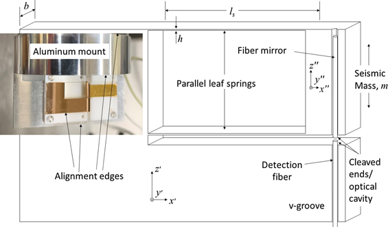
Figure 2. Sketch of the fused silica oscillator that is the sensing element of the accelerometer shown in the inset photo.
Download figure:
Standard image High-resolution image2.1. Sensor fabrication, design parameters, alignment and predicted versus as built frequency
The mechanical oscillator is fabricated from a single wafer of fused silica using a laser assisted etching process that is commercially available [15–17]. The fabrication technique is limited to fused silica, and achieves deep, precise etches of thin wall (500/1 aspect ratio is possible) three-dimensional structures on the scale of several millimeters, with at least one vendor claiming precision and repeatability below 1 µm [16].
The monolithic, fused silica structure of the sensor includes v-grooves on the frame and the seismic mass for the alignment of cleaved fiber mirrors. The grooves are parallel to the motion axis and perpendicular to the alignment edge of the frame, as illustrated in figures 1 and 2. The dynamic mechanical properties of the sensor can be estimated from physical dimensions during the design phase using the material properties of fused silica assuming typical values of density ρ = 2200 kg m−3 and modulus of elasticity, E = 73 GPa. Two types of sensors were designed; both designs employ the same seismic mass which includes the added mass of a 7.5 mm long optical fiber mirror that serves as the moving mirror of the fiber optic cavity (dimensional drawings are in the supplemental materials). Parameters for three examples are shown in table 1.
Table 1. Nominal sensor parameters.
| Parameter | Sensor S1 (high frequency) | Sensor S2 (high frequency) | Sensor S3 (low frequency) |
|---|---|---|---|
| Wafer thickness b | 0.50 mm | 0.50 mm | 0.50 mm |
| Leaf width h | 0.085 mm | 0.085 mm | 0.020 mm |
| Leaf length ls | 7.50 mm | 7.50 mm | 7.50 mm |
| Calculated mass, m with ρ = 2.2 g cm−3 | 8.19 mg | 8.19 mg | 8.19 mg |
Calc. stiffness  and E = 24 GPa and E = 24 GPa | 106.3 N m−1 | 106.3 N m−1 | 1.34 N m−1 |
Calc. resonance frequency 
| 573.4 Hz | 573.4 Hz | 64.4 Hz |
| Measured resonance frequency | 565.8 Hz | 573.027 Hz | 68.3 Hz |
The accelerometer dynamics are approximated using a simple harmonic oscillator having the frequency spectrum,
where a(ω) is the acceleration amplitude of the table at a sinusoidal excitation with angular frequency ω, Δl(ω) is the motion of the seismic mass relative to the frame measured by changes in fiber optic cavity length l, SI(ω) is the single degree of freedom model of the sensor frequency response function, and ζ is the damping ratio. For a lightly damped system, ζ < 0.03, so that the low frequency approximation  deviates from the full analytical expression by less than 1% for frequencies <0.1ω0. This approximation is common in accelerometry and is the bandwidth selected for our verification testing.
The oscillators are glued to a ceramic alignment jig and a fiber interferometer attached as in references [7, 8]. The combination is screwed to an aluminum mounting block to complete the sensor mechanical assembly shown in figure 3. Both the ceramic alignment jig and the aluminum mounting block have reference surfaces for aligning the components during assembly that facilitate mounting and orienting the sensor on a shaker. Based on these alignment surfaces, the parallelism of the leaf springs, and the alignment of the v-grooves, the reference optical axis z and its primed coordinates are parallel to within far less than the 100 mrad necessary to maintain relative cosine errors below the targeted 1%. However, the performance of the parallelogram as a linear guidance mechanism is difficult to characterize experimentally, as is the geometry of the leaf spring cross section, so that it seems imprudent to claim any greater accuracy without evidence beyond a visual inspection of the gross geometries and stated manufacturing tolerances. Finally, a tunable laser light source [18] is fiber coupled to the optical cavity, and a preliminary signal established using techniques described in [11]. The tunable light source was informally checked, and the value specified by its wavelength controller was found consistent with a known atomic reference to within a few picometers.
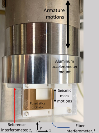
Figure 3. Assembled accelerometer comprising the fused silica oscillator (coated for visibility), ceramic alignment jig, and aluminum mounting block. The red line indicates the reference interferometer path during yaw test of the shaker.
Download figure:
Standard image High-resolution imageThe fully assembled sensor S1 was mounted on a rotation stage to test the alignment through coarse changes in sensor orientation with respect to gravity. A bubble level was used to align the outermost reference surface of the aluminum accelerometer mount to gravity to within <30 mrad. Tilts of 100 mrad on either side of the vertical orientation produced a decrease in the static deflection signal, confirming that the sensor and its mounting fixtures are aligned to at least within the targeted precision.
Assembled sensors were also mounted on a shaker to measure their natural frequencies and damping. An amplitude spectrum response to sinusoidal base excitation is shown in figure 4. Evidence of sidebands, perhaps from a non-linear or transient response coupling to the nominally 1 Hz primary resonance of the shaker, were evident in some plots, as in the S2 response curve of figure 4. The sidebands did not seem to degrade the determination of the sensor dynamic properties and were not investigated. The as-built natural frequency fn = 573.027 Hz for S2 is associated with a damping ratio ζ = 0.000 23. The agreement between designed and as-built natural frequency is exceptional in this case, but a coincidence, since S1, an 'identical' fused silica oscillator obtained months earlier has an as-built frequency of 565.8 Hz. Nevertheless, the variance is well within fabrication tolerances, since the dimension h might vary by as much as 10−5 m, which is the precision claimed by the manufacturer [15]. S3 has an as-built frequency of 68.3 Hz; again, well within stated manufacturing tolerances. Sensors S2 and S3 were damaged during this testing phase, illustrating a need for better packaging and handling. All further results we report are for S1.
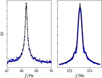
Figure 4. Motion of the seismic mass near the resonance frequency. Plotted is the amplitude l in arbitrary units. On the left is data taken with S3, on the right S2. The blue points are measured data and the black lines are fits to the damped harmonic oscillator. In the left plot the black line corresponds to a harmonic oscillator with f0 = 68.3 Hz and ξ = 0.000 86. For S2, the fit line corresponds to f0 = 573.027 Hz and ξ = 0.000 23.
Download figure:
Standard image High-resolution image2.2. In situ calibration and performance characteristics
The optical cavity of the optomechanical accelerometer of figure 2 is formed between the cleaved end of the detection fiber and a fragment of a similar cleaved fiber mounted in the v-groove on the seismic mass to create a glass/air/glass cavity with nominally 4% reflectivity mirrors, as shown. This plano–plano low-reflectivity cavity is employed to establish an optical cavity axis that is aligned through reference to the fiber cylinder axis, since the plane mirrors are formed using perpendicular fiber cleaves.
The fibers, and by extension the optical axis, align to the mechanical coordinates through placement in the v-grooves. The layout of the fiber interferometer optical components is shown in figure 5 and are listed in the supplementary materials. The optical components form a simple homodyne interferometer that has been described previously [9–11, 19] but which we summarize next, for convenient reference.

Figure 5. Layout of optical components.
Download figure:
Standard image High-resolution image2.2.1. Optomechanical sensitivity, theory
The intensity of laser light reflected from a fiber optic cavity can be measured as a photodetector voltage, V, and treated as a function of cavity length and laser wavelength, V(l, λ), having the form of an Airy function [10]. Assuming the symmetric pair of parallel plane fiber mirrors each have reflectance R, we have

with

where V0 is a constant offset introduced as a fit parameter to account for experimental imperfections (e.g., misalignments), VA is the magnitude of the observed interference fringe and is proportional to (1 + R)2, φ is the interference phase, k = 2π/λ is the wavenumber, l is the cavity length, which is a direct measure of the separation between the seismic mass and the frame, and  the Gouy phase. The wavlength λ is the wavelength in the medium, here air with and index of refraction of n ≈ 1.000.
For a given nominal wavelength λ, the interferometer sensitivity to small displacements of the seismic mass about equilibrium cavity length l0 can be computed from the partial derivative,
Likewise, for calibration purposes, the interferometer sensitivity to perturbations in wavelength can be computed using the partial derivative with respect to λ,
The relative contribution of the derivative of the Gouy phase is negligible (<0.6%) and both sensitivities are evaluated at the same conditions, so that we write

We employ the interferometer during experiments to sense motion of the seismic mass, Δl, in terms of intensity variations, ΔV, with the wavelength tuned during the experiment to λ = λ0 as described in the next section. The slope, r, of the intensity function under these experimental conditions and assumptions is

So that Δl is simply

And by substitution in equation (1)

The optomechanical in situ calibration consists of experimentally measuring the slope, r, or optomechanical sensitivity so as to accurately state the optomechanical acceleration sensitivity SI(ω)/r.
2.2.2. Optomechanical sensitivity, experimental methods
This section is concerned with the measurement of the optomechanical sensitivity, the slope r, that is used to convert changes in light intensity to acceleration according to equation (9). The value of r can be quantified using either of two complimentary techniques named static and dynamic determination of the optomechanical sensitivity. Both methods should yield the same results. Nevertheless, as is discussed further below, each method has their distinct advantages and disadvantages in this application, and it is a further aim of this section to explore these differences and compare uncertainties.
We begin by noting that the optomechanical acceleration sensitivity depends on two mechanical properties of the sensor, the cavity length and the resonance frequency. In fact, it is necessary to measure these two parameters first, and it is a good practice to measure them whenever a sensor is mounted or reoriented on a structure or shaker, or whenever the accelerometer experiences a change in ambient temperature exceeding a few degrees C.
For the static method, the length of the cavity is determined by sweeping the wavelength of the laser source. Figure 6 shows the intensity measured at the output of the interferometer for a sweep ranging from 1450 nm to 1640 nm. For a large wavelength range starting at 1500 nm and ending at 1600 nm, the fringe amplitude is consistent. At the ends of the range the fringe visibility degrades. The points near the interference minima are plotted in black. The location of the minima can be used to obtain the cavity length. The minima of equation (2) occur at 2kl0 = (m + moff)2π, where m is an integer denoting the order of the minimum. Since the absolute order of the minimum is not known, an unknown offset moff is included. This equation can be rewritten to


Figure 6. Sweeping the wavelength of the tuneable laser over its entire range. For this experiment the shaker was not driven, the seismic mass is only driven by thermal motion and seismic motion that is present in the laboratory. The fringe amplitude and voltage at the minima is reasonably stable in the wavelength range from 1500 nm to 1600 nm. The location of the minima can be used to predict the cavity length. Fifty points around the minima are plotted in black.
Download figure:
Standard image High-resolution imageHence the slope of the plot of λmin −1 vs m is 1/(2l0). Figure 7 shows the measured values of λmin −1 as a function of m together with a straight line fit to the data. The agreement between the data and the fit in the wavelength range from 1500 nm to 1600 nm is outstanding as can be seen by the residuals plotted in the lower panel of figure 7. The slope of the fitted line yields a cavity length l0 = 121.311 µm ± 0.0001 µm.

Figure 7. Location of the minima as a function of order m. Here the minimum near 1640 nm has been designated to be m = 1. With decreasing wavelength m increases. The blue data points correspond to the minima found at wavelengths between 1500 nm and 1600 nm. The black line is a straight-line regression to the blue data points. The lower plot shows the difference of the measurements to the line in the same units as the plot on the top. From the slope a cavity length of l0 = 121.311 µm is obtained.
Download figure:
Standard image High-resolution imageThe resonance frequency of the seismometer is obtained by exciting the shaker with frequencies near the estimated resonance frequency. Usually a sweep with constant amplitude over a few hertz is carried out. Figure 4 shows two such sweeps for the sensors S2 and S3. The resonance frequency is readily obtained from the largest amplitude. Note this determination does not require the intensity to be calibrated as displacement. After the free resonance frequency and the cavity length have been determined, the approximate working point in wavelength λ0 is selected. The working point is optimal on the steepest slope of the data, which we refer to as the quadrature point. The sign of the slope is irrelevant for this task. Here, we use λ0 = 1561.845 nm.
For the static method to determine the optomechanical sensitivity, the wavelength must be scanned around the quadrature point such that the measured intensity at the output port goes through a full fringe, which works out to be a scan from λ0 − Δλ to λ0 + Δλ, with  . A subset of the data taken for the long wavelength sweep can be used for this analysis. Figure 8 shows such data. A non-linear fit to equation (2) is performed (note that Ψ(l, λ) is neglected and set to 0) with fit parameters V0, VA, R and l = l0. Good starting points for these four values are
  , and the l0 obtained above, here 121.311 µm. The results for these parameters obtained by the non-linear fit are shown in table 2, and the resulting function plotted versus the data in figure 8. The difference between the measured values are shown in the bottom graph of figure 8. The residuals are dominated by low amplitude higher frequency periodic variations arising from the presence of other parasitic cavities. These parasitic cavity responses are also visible in the inset of the figure. The parasitic responses correspond to two cavities with lengths of 5.57 mm and 4.18 mm, respectively, that we speculate are within the fiber mirror mounted on the seismic mass. Finally, the values of the static fit parameters and their uncertainties are shown in table 2 along with the static optomechanical sensitivity obtained from equation (7) and its uncertainty.
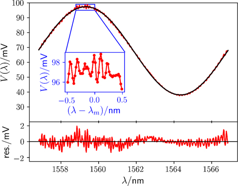
Figure 8. Data used for the static determination of the optomechanical sensitivity. The red points in the top plot shows the measured wavelength over one fringe symmetrically located around the quadrature point, 1561.843 nm. The black line is a fit to equation (2) with the Gouy phase set to zero. The bottom plot shows the residuals of the fit. The residuals are dominated by oscillation with a period of 0.1094 nm that beats with a second oscillation with a period of 0.1458 nm. These periods are consistent with parasitic cavities of lengths 5.57 mm and 4.18 mm. The blue coordinate system in the inset show a zoom near the maximum.
Download figure:
Standard image High-resolution imageTable 2. The parameters obtained by the static and dynamic calibration. The uncertainties are the standard deviation of calibrations repeated at fixed operating conditions.
| Static calibration | Dynamic calibration | |||
|---|---|---|---|---|
| Parameter | Value | 1σ Uncertainty | Value | 1σ Uncertainty |
| V0 | 38.06 mV | 0.05 mV | 38.20 mV | 0.011 mV |
| VA | 30.05 mV | 0.07 mV | 30.25 | 0.015 mV |
| l0 | 121.2370 µm | 0.0001 µm | 121.2483 µm | 0.0001 µm |
| R | 0.007 | 0.001 | 0.014 | 0.001 |
| Calculated result | ||||
| r(121.237 µm) | 238.47 mV µm−1 | 0.25 mV µm−1 | 236.44 mV µm−1 | 0.06 mV µm−1 |
For the dynamic method, the wavelength of the laser remains fixed at λ0. The shaker is driven at the free resonance frequency of the optomechanical sensor such that the interferometer goes through at least one full fringe, i.e., the motion amplitude is at least a quarter of the wavelength, here 390 nm. The data is sampled as a function of time and a model with a harmonic oscillation is fit to the measured data. See the appendix

Figure 9. The top plot shows the measured voltage at the interferometer output as a function of time. The black line is obtained from the fit model detailed in the appendix
Download figure:
Standard image High-resolution imageThe methods are compared side by side in table 2 and figure 10. Values of the optomechanical sensitivity r appear discrepant. The difference between the two values obtained is greater than the 1 sigma uncertainty bounds, suggesting that there are systematic differences between the methods not captured by our model of the measurement process. We conclude that either one of both these uncertainties may be missing at least one component, or that components have been misestimated. Because unknown systematic effects seem more likely than misestimates of any values in table 2, we add a 'dark' relative uncertainty component of 0.5% to each method's budget to acknowledge that there are factors yet to be accounted for (see reference [20] for a discussion of dark uncertainty in the context of a comparison).

Figure 10. Comparison of the static calibration (red points) to the dynamic calibration (cyan points). The data in the calibration is measured as a function of wavelength. The data for the dynamic calibration is measured versus time. Here both data sets are plotted as a function of kl, half the phase in the cosine of equation (2).
Download figure:
Standard image High-resolution imageIn a qualitative sense, the chief disadvantage of the static method is a reliance on a laser that can be tuned through a large range of wavelengths/frequencies. A second potential problem is that the method seems susceptible to parasitic cavities. The contribution of the parasitic cavities to the overall intensity is a function of wavelength that has the potential to bias determination of the static fit parameters. Nevertheless, the static calibration can be performed with nothing more than an oscilloscope and a reference quality tunable laser (e.g., calibrated wavelength and/or wavemeter) making it convenient. Qualitatively, the dynamic method result is more precise, avoids the problems of parasitic cavities, but is computationally intensive and requires a mechanism to excite the accelerometer at its resonance frequency. Since the data in this article were taken with a fully automated data acquisition system, and a shaker was already employed, the dynamic calibration method was preferred, since it appears more precise and the residuals more random.
3. Electrodynamic shaker
The electrodynamic shaker is shown in figure 11, and was fashioned from a commercially available weak motion, electromagnetic seismometer (Teledyne Geotech S/13 Seismometer [21]) purchased in used condition. While an unusual choice, it was convenient given the limited access to NIST laboratories and equipment during 2020. It also served to demonstrate that a fully functional primary system can be fashioned quickly, even by those lacking the resources of a National Metrology Institute. The seismometer/shaker has been oriented to translate horizontal to gravity, and its housing removed. Large coil springs that support the moving magnet armature in the vertical orientation were removed to improve access. The calibration coil assembly was also removed, so the seismometer function is not calibrated, but is useful nonetheless for qualitative diagnostics of the ambient seismic environment. An adaptor plate of soft iron was fashioned and screwed on to the armature in place of the calibration coil assembly, the soft iron acting as a pole piece to help shunt the remaining calibration coil magnetic circuit. The plate also has a threaded hole (UNF 10-32) to facilitate stud mounting of the device under test. The aluminum accelerometer mount is equipped with a similar threaded hole, and was stud mounted to the shaker, oriented so that the fused silica oscillator lay in the x, z plane, and so that the seismic mass translates along the armature axis. A commercial laser interferometer [22] is employed to measure the armature displacement. The laser is referenced to an acetylene absorption line via a gas cell that is part of the integrated laser interferometer system [22] providing absolute traceability to the meter. This laser was also used as an informal reference to check the wavelength controller of our tunable laser. The vacuum-wavelengths of the two lasers matched when the tunable controller was set to 1534.0955 nm, which correlates with an acetylene absorption line at 1534.0986 nm.

Figure 11. Commercial seismometer employed as shaker (a) outer housing (b) housing removed showing elements of seismometer/shaker (c) location of laser interferometer used to measure armature motion relative to optical table.
Download figure:
Standard image High-resolution image3.1. Shaker characterization and performance
The voice coil is excited by applying fixed sinusoidal voltages of chosen frequency and amplitude. Current in the voice coil produces a force on the suspended magnet system causing the armature to oscillate along the seismometer axis, which is kinematically constrained by the arrangement of suspension flexures (delta rods [21]) visible in figure 11. The rigid-body motion of the magnetic armature along this direction is recorded by directing the reference laser interferometer at a plane mirror affixed to the accelerometer mount, normal to the axis of motion, and offset from the centerline of the shaker and the accelerometer by approximately 10 mm in the −x direction. Pitch motions about the x-axis can lead to offset (Abbé) errors in the recording of the platform motion by the interferometer at this location, since rotations about x are indistinguishable from translations in z. Pitch motions about the x axis also tilt the sensor, leading to further spurious response from the accelerometer. Offset errors also result from motions about the y axis.
A complete characterization of the armature motion as a function of frequency, amplitude, load, etc, is beyond the scope of this investigation. We attempted to bound the influence of potential yaw and pitch errors on the acceleration comparison by measuring the platform motion as a function of excitation frequency at two locations, one on axis and one offset, first in x, then in y. Phase measured between the two locations was consistent in sign through the measurement bandwidth between 5 Hz and 30 Hz, suggesting that the shaker table motion was rigid to first order. The ratio of displacements recorded near the centerline of the armature and near the outer edge of the accelerometer mount appeared to cause deviations in relative amplitude by as much as 0.4% at frequencies around 30 Hz, indicative of small yaw and pitch motions caused by a resonance in the shaker. We chose to perform all calibration experiments in a bandwidth below this resonance to avoid these errors.
Another potential source of error was the lack of a true inertial frame for the reference laser interferometer in our experimental set up. The diagram of figure 12 illustrates a worst-case scenario that we experienced when we initially mounted both the reference laser and the shaker on the same table, as shown in the photo of figure 11. Given the approximate mass of the table mot = 500 kg and assuming a horizontal table resonance of 10 Hz, we employ known values for the shaker mass, ma = 5 kg with resonant frequency fs = 1 Hz [21], and the sensor seismic mass m = 8.19 mg and resonant frequency, f0 = 573 Hz to calculate a qualitative response in figure 13. This toy model indicates that the sensor accelerates due to motions of the optical table (e.g., from shaker recoil) that are not observable by the reference laser. This error is avoidable if the reference laser is mounted on a platform isolated from the shaker, a standard practice that we neglected. Lacking a convenient means to achieve separate inertial frames for reference laser and shaker in our ad hoc calibration lab, we opted to locate both shaker and reference laser on the laboratory floor. While this is again a shared reference frame, acceleration from shaker recoil was no longer evident.

Figure 12. Lumped parameter model of accelerometer (m), shaker (ma), and optical table (mot) primary modes of horizontal vibration.
Download figure:
Standard image High-resolution image
Figure 13. The ratio of accelerations observed by the accelerometer and reference laser interferometer in response to voice coil excitation for the model of figure 12.
Download figure:
Standard image High-resolution image4. Comparison experiments
Shaker motions were varied in a systematic fashion to explore the accuracy of the accelerometer under test as a function of amplitude and frequency. Six comparison tests were performed at fixed acceleration levels of 0.01 m s−2, 0.03 m s−2, 0.06 m s−2, 0.1 m s−2, 0.3 m s−2 and 0.6 m s−2. Each test comprised a series of single frequency excitations ranging from 2 Hz to 30 Hz in 1 Hz steps. The accelerometer under test was characterized to determine its quadrature point and slope r prior to each test using methods previously outlined. The accelerations observed using the reference laser interferometer and as observed by the accelerometer under test were recorded at each test frequency, and the average amplitude response of each was computed by fitting to a sine wave over a sample window that was scaled to automatically capture at least 10 sinusoidal oscillations. The data were also postprocessed and a correction applied using the fitted Airy function to capture the full non-linear dependence of sensor output on cavity displacement. A plot of the ratio of average acceleration amplitudes in figure 14 shows that agreement between the armature acceleration measured using the reference interferometer and that measured by the accelerometer is generally very good. The agreement for all amplitudes appears to be near our target of 1% relative accuracy. We note that the standard deviation indicated by the error bars in the data improves as acceleration increases beyond 0.03 m s−2. Precision above 0.06 m s−2 is such that an offset is clearly apparent. This suggests a systematic discrepancy, with the sensor overstating the acceleration on the order of 1% relative to the reference interferometer value. This discrepancy is evident in all the data, but somewhat obscured by scatter in the smallest amplitudes tested.
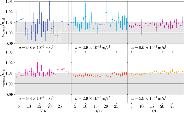
Figure 14. Relative amplitude of shaker table acceleration: optomechanical accelerometer response with respect to reference interferometer for frequencies between 2 Hz and 30 Hz with experiment mounted on the laboratory floor. The data points are averages (unweighted means) from five frequency sweeps. The uncertainty bars are the standard deviations from the obtained data. For the highest acceleration only half that amount of data was available.
Download figure:
Standard image High-resolution image5. Conclusions
The results in figure 14 suggest that the existing primary and the new optomechanical methods are equivalent to within 1% relative uncertainty using the sensor and techniques presented. Further, we present evidence that raw sensing elements can be designed, manufactured, and subsequently assembled into accelerometers deviating less than 2% from design parameters using commercially available discrete part manufacturing. Reference accelerometers of this sort might be routinely made using this type of discrete part fabrication that would conform to international values of acceleration within 2% without recourse to any sort of shaker testing. Clearly, many more samples and design iterations are required, but the potential to infer the sensor frequency/sensitivity accuracy simply from manufacturing tolerances is readily apparent. Far more speculatively, we note that this manufacturing process is available as a standalone machine [16], analogous to a 3D printer, so it is quite conceivable that one might simply print reference accelerometers having uncertainties on a par with the best primary calibration labs, if a suitable light source and fiber optic components can be obtained. Compact tunable lasers locked to atomic frequencies are not yet commodities but are readily available as general-purpose optical test instruments for telecommunications applications.
The seismometer employed here as a shaker proved remarkably convenient for this purpose. The translational constraints of these instruments seem more than adequate, giving few indications of problematic off axis excursions in our limited experimental investigations of yaw and pitch errors. Evidence of a shaker resonance was noted around 30 Hz, and we suspect that this caused a deterioration of the 10−2 m s−2 comparison data at the higher frequencies. We feel confident that the comparison data of figure 14 is accurate and precise enough to conclude that there is a systematic offset of the in situ calibrated optomechanical result, independent of the shaker limitations.
The optomechanical result appears to overestimate the table acceleration by 1% relative to the shaker test throughout the range of frequencies. Recall that the question when employing such a scheme as an acceleration reference boils down to one of fidelity: are the sensor dynamics adequately captured by the single degree of freedom approximation of figure 1, where the accelerometer base, the shaker table, and the interferometer all experience the exact same motion? The answer here appears to be a qualified no since the comparison reveals an offset at the level of a percent. While the offset could arise from a variety of sources, our present hypothesis is that error motions and other modes of vibration render the single degree of freedom approximation of the sensor response function inadequate if one seeks relative accuracy below the percent level [23], which is desirable given the relative ease and precision of the optomechanical calibration method. The sensor response function is critical to the determination of the slope r when using the dynamic method which we employed during the comparison, and it may be that the discrepancy of table 2 is further evidence that the single degree of freedom approximation is insufficient to achieve relative accuracy beyond the percent level for this particular oscillator design.
The equipment and procedures we developed for comparing primary acceleration calibration and the new in situ calibration approach inspired the development of the dynamic calibration technique described in the appendix
Acknowledgments
We thank Douglas T Smith for loan of the tunable laser, Gordon A Shaw III for loan of the reference interferometer, and Patrick Egan for calibration checks of critical optical wavelengths. As ever, the work would not be complete without the outstanding support of the NIST machine shops.
Appendix A
Here we describe a method to obtain the parameters of the optomechanical cavity from measured values of the light intensity, converted by a photodetector to voltage, as a function of time. The goal is to find the slope r discussed in the main text. This slope is necessary to convert voltage amplitude to acceleration.
A.1. Principle
We excite the accelerometer at its resonance frequency so that motions of the seismic mass with respect to the frame cause changes in the optomechanical cavity length that exceed λ/4. The dynamic waveform of the sensed voltage is sampled at a frequency that is large compared to several multiples of the frequency of oscillation. We further assume that the wavelength of the laser λ is known, and, furthermore is set to a value such that with the sensor at rest, the cavity is at quadrature, i.e., the light intensity is half between constructive and destructive interference.
The cavity length as a function of time for single frequency excitation is assumed to take the form of a simple sinusoid,

where the parameters to be identified are l0 the cavity length at the equilibrium position of the oscillator,  the amplitude of oscillation with A > λ/4, and
  the phase of the oscillation.
The voltage observed at the photo detector is

with V0 denoting the voltage measured during destructive interference. The additional fit parameters, are A, ϕ, l0, R, and VA denoting the amplitude and phase of the oscillation, the cavity length, the reflectivity, and the amplitude of the fringe, with V0 + 2VA being the voltage found at constructive interference. The wavenumber k = 2π/λ and the resonant frequency of the oscillator ω0 is known. The fit of equation (A2) to the measured data is difficult, because the functional dependence of three out of the six fit parameters is non-linear. The non-linear fit can be executed if good initial values for the parameters are supplied. Section A.2 of this appendix explains the process of finding these.
Once decent starting values for the parameters are supplied, a non-linear fitting routine can be used to obtain estimated values for the parameters. Table A1 shows the values obtained from the fit and their uncertainties. The uncertainties are obtained from the covariance matrix of the fit.
Table A1. Initial guesses and final values of the parameters used to parameterize the function given in equation (A2).
| # | Parameter | Initial guess | Source of initial guess | Final value | Uncertainty |
|---|---|---|---|---|---|
| 1 | V0 | 37.849 mV |
![$\mathrm{min}[V\left(t\right)]$](https://content.cld.iop.org/journals/0026-1394/58/5/055005/revision4/metac1402ieqn9.gif)
| 37.781 mV | 0.09 mV |
| 2 | VA | 30.245 mV |

| 31.035 mV | 0.12 mV |
| 3 | z0 | 121.2420 µm | Known or λ sweep | 121.2365 µm | 0.2 nm |
| 4 | A | 0.4120 µm | Equation (A4) | 0.4171 µm | 0.2 nm |
| 5 | φ | −0.5596 | Equation (A5) | −0.5313 | 0.0006 |
| 6 | R | 0.04 | Assumed to be 0.04 | 0.017 | 0.002 |
| Result r | 0.2415 V m−1 | 0.0005 |
Figure A1 shows V(t) sampled for two oscillations with a sample rate of 30 kHz. The wavelength is λ = 1.561 84 µm ± 0.000 01 µm and the forced oscillation frequency is f0 = ω0/(2π) = 565.8 Hz. The data shown contains 106 data points and the best fit yields a residual sum of squares of 1.17 × 10⁻⁵ V2. This number is consistent with an individual uncertainty of 342 µV per data point.

Figure A1. The measured voltage on the photodetector as a function of time when the seismic mass displaces more than a full fringe.
Download figure:
Standard image High-resolution image
Once, the estimates for the parameters are obtained with the non-linear fit, the slope r at l = l0 can be obtained with three parameters using,

For the parameters shown in table A1, a value of r = 0.2415 V m−1 with an uncertainty of 0.5 mV m−1 is obtained.
A.2. Estimating initial values
We use symbols  and
and  to describe the initial guesses for the parameter before applying the non-linear fit. The voltages
  and
and  are estimated from the minimum, Vmin, and maximum, Vmax, of the measured voltage in the measured interval using
  and
and  . The value
  is known from the type of sensor used. It can also be inferred from a wavelength sweep without excitation, as described in the main text. The reflectance of mirrors used in the cavity is about
  , which is a good value to start the fit.
In order to obtain  and
and  , we rewrite equation (A2), by assuming R is equal to zero and that the optomechanical sensor is operated at the quadrature,
  , where m denotes an integer. In that case, equation (A2) simplifies to

The sign before the sine depends on the working point that was chosen. The measured voltage can either decrease or increase when the cavity length is increased by a tiny amount. The maximum value of the time derivative of  is
is

For the positive sign in the sine in equation (A4) the maximum in the derivative occurs at

For the negative sign the maximum is at

A.3. Conclusion
The procedure discussed here provides estimate values for the parameters that can be used to fit the measured light intensity as function of time. The first estimate is already very good, but the non-linear least-squares fit can be used to refine the estimate to greater precision.
Footnotes
- 1
Of necessity, certain commercial equipment, instruments, or materials are identified in the paper and references in order to specify the experiments adequately. Such identification is not intended to imply recommendation or endorsement by the National Institute of Standards and Technology (NIST), nor is it intended to imply that the materials or equipment identified are necessarily the best available for the purpose.