

Abstract
We used absolute primary acoustic gas thermometry (AGT) to calibrate a Pt–Co resistance thermometer on the thermodynamic temperature scale by measuring the speed of sound in helium at a temperature T* chosen to be near the temperature of the triple point of neon, TNe. Prior to the present AGT, the Pt–Co thermometer was used with a neon triple-point cell as part of an interlaboratory comparison. Taken together, the results of the interlaboratory comparison and the present AGT redetermined the thermodynamic temperature TNe = (24.555 15 ± 0.000 24) K. This new value of TNe is consistent with other recent determinations obtained with various primary methods. After completing the AGT thermodynamic calibration, we used the Pt–Co thermometer to link T* to the temperature ratios measured by single-pressure refractive-index gas thermometry (SPRIGT) in a different laboratory. (Gao et al 2020 Metrologia 57 065006) Now, the T*-linked SPRIGT system can calibrate other thermometers on the thermodynamic temperature scale T in the range 5 K ⩽ T ⩽ TNe without using the international temperature scale ITS-90. At most temperatures in this range, the uncertainties of the T*-linked SPRIGT system are smaller than those of the ITS-90 systems used by National Metrology Institutes to calibrate resistance thermometers.
Export citation and abstract BibTeX RIS

Original content from this work may be used under the terms of the Creative Commons Attribution 4.0 licence. Any further distribution of this work must maintain attribution to the author(s) and the title of the work, journal citation and DOI.
1. Introduction
Using the techniques of primary acoustic gas thermometry (AGT), [1, 2] we measured the thermodynamic temperature of the triple point of neon and obtained the result: TNe = (24.555 15 ± 0.000 24) K. (All uncertainties reported in this work are one standard uncertainty corresponding to a 68% confidence level.) As shown in table 1 and figure 1, the present result for TNe is consistent, within combined uncertainties, with other recent determinations of TNe [3–6].
Table 1. Recent determinations of TNe.
| Reference | Year | Method | TNe K | u(TNe) mK |
|---|---|---|---|---|
| [3] | 2006 | AGT | 24.555 15a | 0.25 |
| 24.555 27a | 0.26 | |||
| [4] | 2017 | DCGT | 24.5561 | 0.28 |
| [5] | 2020 | RIGT | 24.555 49 | 0.43 |
| [6] | 2020 | RIGT | 24.555 41 | 0.29 |
| This work | 2020 | AGT | 24.555 15 | 0.24 |
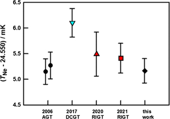
Figure 1. Values of TNe from the literature and from this work. Literature values are identified, by technique, first author, year, and reference:  AGT Pitre et al (2006) [3];
  DCGT Gaiser et al (2017) [4];
  RIGT Rourke (2020) [5];
  RIGT Madonna-Ripa et al 2021 [6]; ⧫ AGT this work.
Download figure:
Standard image High-resolution imageIn figure 1, two literature values of TNe are based on refractive-index gas thermometry (RIGT) [5, 6] and one is based on dielectric constant gas thermometry (DCGT) [4]. These values of TNe were obtained during wide-range measurements of the differences T − T90 and their estimated uncertainties u(T − T90). However, these references do not include values of u(TNe), We consulted the respective authors who graciously provided u(TNe). In 2006, two of the present authors (LP and MRM) obtained two values of TNe using primary AGT [3]. (The two 2006 AGT values differ, in part, because they were traced to two different neon triple point cells.) The present AGT uses completely new hardware and software and a different neon triple-point cell. Furthermore, the present apparatus was not operated by LP and MRM. Thus, the 2006 AGT value of TNe and the present AGT value are uncorrelated.
Our acoustic measurement of the thermodynamic temperature near TNe is preliminary and a key part of the program of Gao et al [7] to use single-pressure refractive-index gas thermometry (SPRIGT) to calibrate secondary thermometers (such as resistance thermometers) in the temperature range 5 K ⩽ T ⩽ TNe. Gao et al measure ratios of thermodynamic temperatures. By linking their ratio measurements to the present value of TNe, we have enabled their system to calibrate secondary thermometers with the thermodynamic temperature without using any input from the internationally accepted temperature scale ITS-90.
To link the SPRIGT to TNe, we determined T* in two successive AGT runs in June and July 2019 at LCM-LNE-Cnam. After completing and analyzing the results of the AGT work, we obtained a thermodynamic calibration of one particular platinum–cobalt (Pt–Co) resistance thermometer, which was transferred to the TIPC-LNE Joint Laboratory of the Chinese Academy of Sciences, where—by September 2019—it was installed in the SPRIGT system to calibrate that system at TNe. As discussed in [7], the uncertainty of the TNe-linked SPRIGT system was 0.16 mK at TNe where it was dominated by imperfections in the AGT and resistance thermometry. (Thus, linking a more accurate value of TNe could further improve the SPRIGT system.) At 5.0 K, the uncertainty of the SPRIGT system was 63 μK; it was dominated by the uncertainty of helium's 2nd and 3rd density virial coefficients B and C.
Figure 2 shows that, in the range 14 K ⩽ T ⩽ TNe, the uncertainties of TNe-linked SPRIGT, primary AGT, and primary DCGT are all substantially smaller than those of T90 as disseminated, for example, by the National Metrology Institutes (NMIs) of France and Italy. [8] In this range, ITS-90 can be realized using two different instruments, the constant volume gas thermometer (CVGT) above 3 K, and the capsule standard platinum resistance thermometer (cSPRT) above 13.8 K. [9] The cSPRT must be calibrated at specific sets of defined temperature fixed points: the e-H2 triple point, two vapor pressure points of e-H2, and TNe. During the last 20 years, no NMI in the world realized the e-H2 vapor pressure points, which gives the cSPRT an uncertainty on the order of 1 mK between these two points. Furthermore, only the NMI of Japan has operating CVGTs. Because operating these CVGTs is complex and time-consuming, these NMIs usually calibrate new thermometers by comparing them to previously calibrated thermometers. To summarize, the realizations of ITS-90 in the range 5 K ⩽ T ⩽ TNe are infrequent, complex, and have larger uncertainties than newer primary thermometers. In this range, newer primary thermometers are competitive with ITS-90.
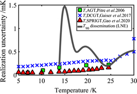
Figure 2. Uncertainties of realizations of T and T90.
Download figure:
Standard image High-resolution imageOur realization of a primary acoustic gas thermometer was a helium-filled, copper-walled, quasi-spherical, cavity resonator. The theoretical principles and experimental techniques for determining TNe with this AGT are well-established [1, 2, 10]. Here, we briefly describe the AGT and our measurements while emphasizing the features that dominate our uncertainty budget.
2. Experiment setup
2.1. Cryostat
The AGT and its pressure vessel were contained within a cryogen-free cryostat cooled by a commercial 4 K pulse-tube cryocooler (Cryomech PT405, 0.5 W at 4.2 K cooling power) 7 . Compared to the cryostat used by Pitre et al in 2006 [3], the cryocooler is advantageous because it has long-term, continuous stability and it avoids the noise generated by boiling liquid helium. Figure 3 is a schematic diagram of the cryostat, which is the prototype of the cryostats used for several primary thermometers [6, 7]. To reduce the radiation thermal load on the pressure vessel surrounding the quasi-spherical resonator, the vessel was surrounded by two gold-plated heat shields attached to thermostatted flanges. When cooling began, a small amount of helium exchange gas (approximately 1000 Pa) was admitted into the sealed space between the shield designated 'heat switch' and the pressure vessel (figure 3). The lowest temperature reached by the pressure vessel was approximately 6 K. The methods for temperature control are the same ones that we used in previous work [7, 11–13]. Referring to figure 3, the finest temperature control of the quasi-sphere was achieved by reading cSPRT-1 with an F18 bridge and feeding the bridge's output through a proportional-integral feedback loop to heater-3. The temperature was monitored by cSPRT-2 using a second bridge. If the thermometry were ideal and if any temperature gradients were time-independent, the differences between the two thermometer readings ΔT2−1 ≡ (TcSPRT-2 − TcSPRT-1) would be time-independent. Averaged over each 12 days-long run, ⟨ΔT2−1⟩Run 2 − ⟨ΔT2−1⟩Run 1 = 3.5 μK. During all the measurements, imperfect pressure control generated very low-frequency fluctuations that were equivalent temperature changes as large as ±20 μK. These pressure fluctuations, together with the temperature fluctuations and possible temperature gradients, contributed 21 μK to the uncertainty of TNe.

Figure 3. Schematic diagram of the cryogen-free cryostat used in this work.
Download figure:
Standard image High-resolution image2.2. Gas handling system
As shown in figure 4, the gas handling system was similar to that used by Pitre et al during their measurements of the Boltzmann constant [14, 15]. In [15], Pitre et al demonstrated that the cold trap and the getter in the fill line reduced the concentration of impurity gases to negligible levels. During most of the AGT measurements discussed in this work, the cold trap was not in use. A few, separate dedicated tests with the cold trap were conducted to check the possible presence and the effect of trace amounts of impurities, as discussed in section 4. The pressure control loop was installed in a temperature-controlled box that limited the maximum temperature excursion to 10 mK around a given set point. Two absolute pressure transducers (Paroscientific Digiquartz 745, full-scale pressure 0.7 MPa) monitored the pressure. These transducers were traceable to the LNE standard. The pressure in the resonator was regulated by one of the pressure transducers and a mass flow controller using a proportional-integral feedback loop written in the LabVIEW® software. A relative pressure stability of 0.5 × 10⁻⁶ was maintained throughout the operating range. As shown in figure 4, a 6 m-long capillary (ID 1.01 mm) connected the gas handling system to the quasi-spherical cavity. The electrical cables surrounded the capillary and were enclosed by a bellows. This arrangement avoided using hermetic feed throughs at low temperatures. On occasions when the cryostat was open at room temperature, valves 8 and 9 were used to flush the inside of the cavity with clean helium, thereby maintaining the cavity's cleanliness. During the measurement at low temperature, helium did not flow through the resonator to reduce the possible heat transfer from the room to the resonator and to minimize the cost of the helium.

Figure 4. Gas handling system. The components in the gray rectangle were enclosed in a thermostatted box.
Download figure:
Standard image High-resolution image2.3. Quasi-spherical acoustic gas thermometer
The acoustic thermometer was the diamond-polished, copper, quasi-sphere known as 'TCU1'. This thermometer was described in detail and studied from a metrological point of view by Sutton et al 2010 [16]. Sutton et al used TCU1 to determine the Boltzmann constant k; their result was within 3 ppm (1 ppm = 1 part in 106) of the final value of k adopted when the kelvin was redefined in 2019. TCU1 has an internal radius of 50 mm and a 5 mm thick wall. (A typical AGT with a 50 mm radius has a 10 mm thick wall.) TCU1's cavity is modeled as a triaxial ellipsoid with axes of length a, a(1 + e1), and a(1 + e2). In 2009, Sutton's microwave measurements determined e1 = 0.001 048 and e2 = 0.000 79 at the triple point of water. In this work, at the triple point of neon, using the TM11 mode, we determined e1 = 0.001 031 and e2 = 0.000 792; using the TM12 mode, we obtained e1 = 0.001 034 and e2 = 0.000 792 The small change in e1 might have resulted either from the movement of a microphone (or some other component of TCU1) or from anisotropic thermal expansion between TTPW and TNe.
2.4. Microwave measurements
Figure 5 is a block diagram of the microwave and acoustic measuring system. We used two straight antennas to measure the resonance frequencies and half-widths of the TM11 and TM12 microwave modes while TCU1 was thermostatted near TNe and immersed in helium. For the TM11 mode, we used 10 pressures ranging from 30 kPa to 110 kPa. For the TM12 mode, the data were much noisier and only two pressures were used: 30 kPa and 70 kPa. From the microwave data, we calculated aeq, the radius of a sphere with the volume equivalent to that of the quasi-spherical cavity at zero pressure. To calculate aeq, we corrected the measured frequencies for the microwave penetration depth, the refractive index of helium, the isothermal compressibility of copper (using the value −V−1(∂V/∂P)T = 19 × 10−8 Pa−1 from [7]), the effects of antennas and the fill duct [17], and the second-order shape correction [18, 19]. The statistical uncertainty of the extrapolated, zero-pressure radius is 0.14 ppm.

Figure 5. Block diagram of the microwave and acoustic measurement system.
Download figure:
Standard image High-resolution imageFigure 6 demonstrates that the values of aeq from from two consecutive runs 1 and 2 were mutually consistent and that the repeatability of a single determination of aeq was approximately 1 part in 107. With this precision in mind, table 2 demonstrates two inconsistencies: (1) the values of aeq measured using the TM11 and TM12 modes are inconsistent by up to 1.0 ppm and (2) the values of aeq,m1 and aeq,m2 differ by up to 2.1 ppm, depending upon the method used to correct the measured frequencies for the microwave penetration depth.

Figure 6. Equivalent radius of quasi-sphere from the frequencies of the TM11 microwave mode. The central red line is the mean radius of runs 1 and 2. The outer black lines lie at ±1 standard deviation from the mean radius.
Download figure:
Standard image High-resolution imageTable 2. Scaled relative deviations aeq from their mean 106 (aeq/⟨aeq⟩ − 1) for two modes using two values of the electrical conductivity of copper σCu. Here, ⟨aeq⟩ = 50.111 506 mm.
| Mode | aeq,m1 | aeq,m2 | aeq,m1 − aeq,m2 |
|---|---|---|---|
| TM11 | −1.11 | 1.00 | −2.11 |
| TM12 | −0.09 | 0.20 | −0.29 |
| TM11−TM12 | −1.02 | 0.79 |
The first correction method determines the electrical conductivity σ of the copper resonator by fitting the half-widths of the TM11z triplet. The three components of the triplet were simultaneously fitted with the result σ = 9.69(3) × 108 Ω−1 m−1. This value of σ and the theory of the resonance half-widths leads to the values of aeq,m1 in table 2. Note: we did not use literature values of σ because impurities and/or mechanical stress in oxygen-free, high-conductivity copper can change its electrical conductivity near 24 K by more than one order of magnitude [20].
The second correction method allows each component of each triplet to have its own value of σ and leads to aeq,m2 in table 2. Method 2 adds the measured half-width of each component of the microwave triplets TM11 and TM12 to the measured frequency of that component. Compared with aeq,m1, the values of aeq,m2 were closer to the values expected from the studies of Sutton et al [16]. Method 2 was used for the final value of aeq. To account of the inconsistent values of aeq between the two methods, we added 4.2 ppm to the total uncertainty in table 5.
At 24 K, the Q of the microwave resonances is three times larger than at 273 K; therefore, there is a higher chance that the microwave resonances were over-coupled to the external instruments and/or that the perturbations of the microwave resonances by the microphones and antennas were relatively more important. We were unable to test these ideas; therefore, we added 4.2 ppm to the uncertainty of a2 eq in table 5 and label this uncertainty 'electrical conductivity of shell'. The ratios gn /fn in ppm for the triplet of the TM11 (x, y, z) are (4.63, 4.71, 4.32) and for the TM12 (2.54, 2.64, 2.41). These values were independent of pressure.
The mode-dependent inconsistencies [in table 2, |aeq,TM11 − aeq,TM12| ≫ ufit(aeq)] were up to 1 ppm near 24 K where ufit(aeq) is the uncertainty due to the fit of the triplet. In contrast, Sutton et al [16], using the same quasi-sphere near 273 K, measured values of aeq for the same modes that differed by only 0.12 ppm.
2.5. Acoustic measurements
Two commercially-manufactured capacitive microphones (GRAS model 40BF) were installed in the cavity's wall so that their diaphragms were flush with the cavity's internal surface. In order to reduce electrical crosstalk between the two microphones, the source microphone was excited with 50 V RMS so that it generated sound at twice the frequency of the sinusoidal driving signal. The driving signal originated in a function generator and was amplified to 50 V RMS by a TEGAM® model 2340 high-voltage amplifier (see figure 5). The second capacitive microphone detected the sound in the cavity resonator. The detecting microphone was connected via a coaxial cable to a preamplifier (a GRAS type 26AC) which was connected to a GRAS type 12AA power supply module located at room temperature. Finally, a lock-in amplifier (Stanford Research Systems SR830) was used to measure the in-phase and out-of-phase acoustic signal. At TNe, this arrangement produced a satisfactory acoustic signal-to-noise ratio i.e. the fractional uncertainty of the resonance frequencies [1] was less than 10 ppm at the lowest pressure: 30 kPa.
We measured the acoustic resonance frequencies f(0,n) and half-widths g(0,n) of the radially-symmetric modes for n = 2, 3, 4, 5, 6, 8, and 9. The n = 7 mode was not included for two reasons. First, the frequencies of the (13, 2) and (0, 7) acoustic resonances overlap at low pressures where the modes broaden. (Ideally, f(13,2)/f(0,7) = 1.0017.) Secondly, the breathing mode of the empty copper shell of TCU1 strongly couples to the (0, 7) mode because both modes are resonant near 18.9 kHz at TNe.
We acquired data in two successive runs, each lasting approximately 12 days. Each run began at 120 kPa; then the pressure was decreased in steps of 10 kPa until the run ended at 30 kPa. After each pressure change, we waited 8 to 12 h for the temperature to stabilize. During the next 12 h, we repeatedly measured the resonance frequencies of the seven selected radial modes in approximately 70 cycles. Thus, each run consisted of approximately 4000 measurements of resonance frequencies.
The measurements were made under isothermal conditions at ten pressures between 30 kPa and 120 kPa. We applied all the corrections described by Moldover et al (2014) [1] to the measured values of f(0,n) and g(0,n).
3. Analyzing acoustic data
We corrected the measured values of f(0,n) for the thermo-acoustic boundary layer (using the theoretical value of the thermal conductivity of helium [21]) and we also applied small corrections for the mechanical compliance of the microphones [22], and the ducts that allow gas to enter and leave the cavity [16], and the ellipsoidal geometry of the cavity, as determined from the measurements of aeq. However, the quasi-spherical copper shell is a complicated, bolted-together object; therefore, we and others [23–25] fit corrections to the measured acoustic frequencies to account for two shell-related phenomena: (1) the temperature jump in the helium gas where it contacts the copper shell and (2) the compliance of the copper shell in response to the radial oscillations of the helium within the shell.
On each isotherm, we represented the pressure dependence of the resonance frequencies (as corrected above) by the function:

First, we discuss the terms in equation (1); then we discuss fitting the acoustic resonance frequencies with these terms.
In equation (1), z(0,n) is the eigenvalue appropriate for the (0,n) mode and A0 ≡ w0 2 is the speed of sound in helium at zero pressure; w0 2 determines the thermodynamic temperature using the relation w0 2 = 5 kT/(3m). k is the Boltzmann constant and m the atomic mass of helium-4. The terms A1 p and A2 p2 account for the pressure dependence of the speed of sound. The parameters A1 and A2 are exact multiples of the temperature-dependent acoustic virial coefficients that have been calculated from the fundamental constants and the laws of quantum mechanics and statistical mechanics. For convenience, we fixed A1(T) at the values that were accurately calculated by Czachorowski et al [26]. Fixing A1 affects neither our determination of TNe nor its uncertainty u(TNe) because the coefficients of p in equation (1) are the sum [A1 + ΔA1,(0,n)] and the uncertainties of ΔA1,(0,n) from the fitting are included in the uncertainty budget. We retained A2(TNe) as a fitted parameter because the uncertainty of the theoretical value of A2(TNe) from [27] appears to be larger than the uncertainty from fitting the present data. Within combined uncertainties, the fitted and theoretical values of A2 are mutually consistent. (See below.) Using the ab initio calculations of the fourth density virial coefficient of helium [28, 29], we crudely estimated A3 p3/A0 ∼ 1 × 10⁻⁶ at our highest pressure; therefore, we omitted A3 p3 from equation (1).
In equation (1) the terms ΔA1,(0,n) p account for the frequency-dependent compliance of the 5 mm-thick copper-walled shell. Equation (86) of reference [30] shows that the compliance of a perfectly-spherical, isotropic shell has the form ΔA1 = constant × [1−(f(0,n)/fbreathing)2]−1, where the constant depends on known properties of the gas and the shell. (In this work f(0,7) ≈ fbreathing ≈ 18.9 kHz.) This prediction for an idealized shell is approximately consistent with our data; however, it does not capture the full precision of the data. Therefore, we decided to fit the data for each (0,n) mode with its own value of ΔA1 which we denote 'ΔA1,(0,n)'.
In equation (1), the term A−1 p−1 accounts for unknown details of the scattering of helium atoms by the wall of the quasi-spherical cavity. Indeed, we do not know if the wall is covered with oxides and/or adsorbed gases and/or molecules of, for example, pump oil. Therefore, we and other AGTs have used phenomenological theories to model gas-wall interactions and their consequences for measurements of acoustic resonance frequencies [31, 32]. These theories predict that the wall-gas heat transfer generated when a sound wave reflects off a wall alters the distribution of helium velocities within a thermal accommodation length la of the wall such that the usual hydrodynamic boundary condition Tgas = Twall no longer applies. Instead, a temperature jump occurs at the boundary. The jump introduces into equation (1) the term A−1 p−1, which for low-density helium in a quasi-spherical shell takes the form

In equation (2), κ is the thermal conductivity of helium and the length la is on the order of the mean free path in the helium. In the AGT literature, the value of h in equation (2) has been obtained by fitting low-pressure speed-of-sound data.
Table 3 lists the relative sizes of the terms in equation (1) in the pressure range of this work and, for comparison, the corresponding values from a recent measurement of the Boltzmann constant [15]. The last column is proportional to the signal-to-noise ratio for measuring the f(0,5).
Table 3. Relative importance of the terms in equation (1) in the present data (first two rows) in the measurement of k (last two rows) from reference [15]. The last column is proportional to the signal-to-noise ratio for measuring the resonance frequency f(0,5)

|

|

|

|

|

|

|
|---|---|---|---|---|---|---|
| 24.5 | 0.03 | 7.5 | 1000 000 | 2108 | 15 | 1.4 |
| 24.5 | 0.12 | 1.9 | 1000 000 | 8433 | 240 | 24 |
| 273 | 0.15 | 9.3 | 1000 000 | 147 | 0.5 | 1.8 |
| 273 | 0.70 | 2.0 | 1000 000 | 685 | 9.9 | 45 |
In table 3, the term A2 p2 is substantially larger at TNe than at TTPW and, as calculated ab initio, the standard uncertainty of A2 is 94 times larger at TNe than at TTPW. Therefore, A2(TNe) must be fitted to our data. Unfortunately, fitting the present data does not determine A−1, w0 2, ΔA1,(0,n) and A2 with satisfactory precision. (We discuss this problem in section 7: Conclusions.) Therefore, we relied on the AGT literature to estimate A−1 and its uncertainty. Reference [32] reviewed the literature prior to 2016 and noted that 0.33 ⩽ h ⩽ 0.43 for helium-4 at TTPW interacting with walls made of stainless steel, oxygen-free high-conductivity copper, and electrolytic-tough-pitch (ETP) copper. More recently, Gavioso et al [24] reported 0.38 ⩽ h ⩽ 0.42 in the range 236 K ⩽ T ⩽ 430 K for helium with ETP copper. With these observations in mind, we assumed h = (0.39 ± 0.05) and fitted our acoustic data twice; once fixing h = 0.34 (equivalent to A−1 = 0.023 m2 s−2 MPa) and a second time fixing h = 0.39 (equivalent to A−1 = 0.019 m2 s−2 MPa). We assume that the w0 2 (h = 0.39) is the most accurate value of w0 2 (and TNe) and that the uncertainty contribution from h to u(w0 2) is ±|[w0 2(h = 0.39) − w0 2(h = 0.34]|.
Now, we describe the iterative procedure for fitting the acoustic data.
(Iter 1) Start by guessing the temperature Ttrial as an initial estimate of TNe. (The guess Ttrial = 20 K is close enough!) With this guess, define the data set:
and the model that will be fitted to the data:

(Iter 2) Using Ttrial, correct the microwave frequencies (for the microwave, penetration depth, the refractive index of helium, etc) and correct the acoustic frequencies (for the thermal boundary layer, ducts, etc). Using the corrected frequencies, minimize the sum
by varying A−1, w0, and ΔA1,(0,n) for each acoustic mode at each pressure. σ2 is the squared standard deviation of the measured squared speed of sound.
(Iter 3) Replace Ttrial with an improved Ttrial obtained from Ttrial = Mw0 2/(γ0 R), where w0 resulted from the minimization, R is the gas constant, M is the molar mass of helium-4 and γ0 ≡ 5/3 is the heat capacity ratio at zero density.
(Iter 4) Repeat steps (Iter 1) to (Iter 3) until the difference between successive values of Ttrial is less than 10−6 TNe.
The iteration converged rapidly; after three iterations, the differences between successive values of Ttrial was 10−4 mK. For run 2, the numerical results of the iterated fit for  , A−1, ΔA1(0,n), and A2 are listed in table 4. We emphasize that neither the iteration nor the theoretical values of A1 and A2 have any relationship to ITS-90.
Table 4. Sensitivity of results to the choice of h. We fit equation (1) to combined data from run 1 and run 2 twice; once fixing A−1 assuming h = 0.39 and once fixing A−1 assuming h = 0.34. The values of A1 were fixed by theory [26]. The last row of the table is the theoretical value of A2 [27].
| h | Value | Value | Uncert | Unit |
|---|---|---|---|---|
| 0.39 | 0.34 | Fixed | ||
| w2 | 85011.900 | 85011.707 | 0.017 | m2 s−2 |
| ΔA(0,2) | −2.77 | 0.32 | 0.51 | m2 s−2 MPa−1 |
| ΔA(0,3) | −3.75 | −0.67 | 0.51 | m2 s−2 MPa−1 |
| ΔA(0,4) | −4.46 | −1.39 | 0.51 | m2 s−2 MPa−1 |
| ΔA(0,5) | −7.37 | −4.28 | 0.51 | m2 s−2 MPa−1 |
| ΔA(0,9) | 19.63 | 22.72 | 0.51 | m2 s−2 MPa−1 |
| A2 | 1414.4 | 1399.5 | 3.4 | m2 s−2 MPa−2 |
| A1 (theory) | 5973.89 | 5973.87 | Fixed | m2 s−2 MPa−1 |
| A−1 | 0.0191 | 0.0226 | Fixed | m2 s−2 MPa |
| T = Mw0 2/g0 R | 24.554 967 | 24.554 911 | 5 × 10⁻⁶ | K |
| A2 (theory) | 1457 | 52 | m2 s−2 MPa−2 | |
aStatistical contribution to standard uncertainty only. bReference [27].
After a preliminary analysis, we removed the (0,6) and (0,8) modes from our analysis because these modes had large, smooth deviations from the five remaining modes. We speculate that the frequencies of the (0,6) and (0,8) modes lay too close to fbreathing to represent the shell's compliance correction as the linear function of the pressure ΔA1(0,n) p. The remaining data set comprised approximately 6000 measurements.
Figure 7 displays the deviations of the data from equation (1) for 5 modes measured during runs 1 and 2 using the parameters in table 4 that resulted from the iteration with h = 0.39. Each plotted point represents the average of approximately 70 measurements for a single mode at nearly-identical temperatures and pressures. Each uncertainty bar is the standard deviation of the 70 measurements from their mean.

Figure 7. Residuals after iteratively fitting TNe, ΔA1(0,n), A-1 in equation (1) to the data for both runs while fixing h = 0.39. The legend identifies each radial mode. The outputs from the iteration are in table 4. Each plotted point represents the average of approximately 70 measurements; the uncertainty bars are the standard deviation of the 70 measurements from their mean. (The standard deviations of the means are (70)1/2 ≈ 8,37 times smaller.)
Download figure:
Standard image High-resolution imageIn figure 7, the relative standard deviation of the averaged data from their mean is 1.51 × 10⁻⁶, which corresponds to 37 μK. The differences between the two runs is a quantitative indicator of the long-term (12 days) stability of the complete measurement system, including any possible impurities in the helium. At each pressure, the relative standard deviation of the data for the five modes from their average value was 0.23 × 10⁻⁶, which corresponds to 5.7 μK. This is a measure of the stability of the measurement system during intervals of 12 h.
Inspection of table 4 reveals that the uncertainties of w2, ΔA(0,n), and A2, as determined by fitting, are much smaller than the differences between the best-fit values of these parameters with h = 0.39 and with h = 0.34. Thus, our assumption that h = (0.39 ± 0.05) is crucial for determining the uncertainty TNe.
It is satisfying that the best-fit value of A2 is consistent with the ab initio calculation by Garberoglio et al [27] Under the assumption h = (0.39 ± 0.05), the uncertainty u(A2)measured is 38% of u(A2)theory.
4. Quality tests
Figure 8 displays a powerful test of our understanding of the acoustic resonator. The theory for the half-widths g(0,n) of the acoustic resonances contains no adjustable parameters. If the theory and the half-width measurements were perfect, the excess half-widths Δg(0,n) ≡ (gmeasured − gtheory) would be zero at all pressures, within combined uncertainties. Any phenomenon that removes energy from an acoustic resonance will increase g(0,n); therefore, values of Δg(0,n) > 0 are measures of imperfect understanding of the resonator. Figure 8 plots averaged values of Δg(0,n) measured during runs 1 and 2 after scaling by the factor 2 × 10⁶/f(0,n). With this scale factor, non-zero values of 2Δg(0,n)/f(0,n) are comparable to fractional errors in TNe, expressed in parts per million. (Similarly, fractional errors in 2 × 10⁶ Δf(0,n)/f(0,n) correspond to ppm errors in TNe.)
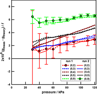
Figure 8. The excess half-widths of the resonances scaled by the factor 2 × 10⁶/f as a function of pressure. Each plotted point represents the average of approximately 70 measurements; the uncertainty bars are the standard deviation of the 70 measurements from their mean.
Download figure:
Standard image High-resolution imageAt corresponding pressures, the averaged values of Δg(0,n) in runs 1 and 2 differed from each other by only a few tenths of a part per million. This reproducibility is comparable to that of w2 in figure 7. (Figures 7 and 8 have equivalent scales.) We fitted the values of 2Δg(0,n)/f(0,n) to linear functions of the pressure. The zero-pressure intercepts for the modes (0,2), (0,3), (0,4), and (0,5) range from 0.4 ppm to 1.8 ppm. (1.8 ppm corresponds to 0.044 mK, which is much smaller than u(TNe) = 0.24 mK.) Apparently, an unknown, pressure-independent energy loss mechanism significantly increases Δg(0,9); however it does not affect f(0,9) as it is show in figure 7.
In prior realizations of AGT, including the use of this resonator filled with argon at TTPW, it was found that Δg(0,n) for many modes increases linearly with pressure [16]. Usually, this increase is attributed to energy losses associated with oscillations of the resonator's shell driven by the radial acoustic oscillations of the gas within the shell.

Figure 9. Pressure dependence of the resistance of the Pt–Co thermometer at TNe. The central horizontal red line is the mean resistance; the outer dashed lines are separated from the mean resistance by ±1 standard deviation corresponding to ±0.036 mK.
Download figure:
Standard image High-resolution image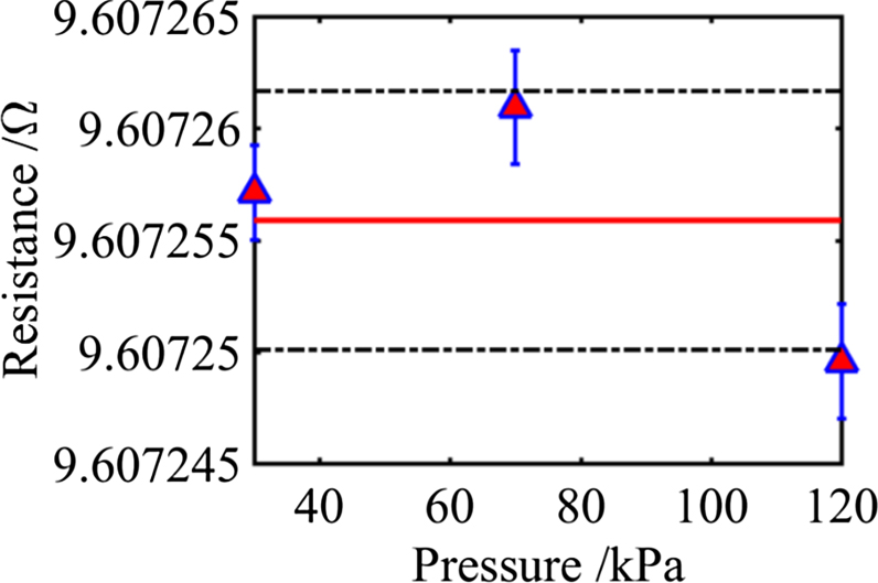
In common with other realizations of AGT, problems in measuring g(0,n) develop as the pressure is decreased. The values of g(0,n) increase (in accord with theory); this increases the overlap of the (0, n) modes with nearby non-radial modes. The increasing overlap with decreasing pressure increases the uncertainty of fitting the resonance frequency and half-widths and introduces bias. The bias has been documented when the (0, 7) mode begins to overlap with the (13, 2) mode [33].
To test for the presence of undetected impurities in the helium, we compared the acoustic resonance frequencies with and without operating the liquid-helium cooled trap shown in figure 4. This comparison is sensitive to impurities at the sub-ppm level and essentially insensitive to the corrections to the acoustic frequencies, the geometry of the shell, etc. First, with helium that passed through the cold trap at ambient temperature, we measured the acoustic resonance frequencies of the cavity near TNe at pressures ranging from 30 kPa to 120 kPa. From this isotherm, we deduced a value of TNe,mix and we measured the resistance of a cSPRT that had a well-known history and sensitivity. To clean the system, we evacuated the pressure vessel and then flushed it three times with helium that had passed through the helium-filled cold trap. Using this 'purified' helium, we remeasured the cSPRT and the acoustic resonance frequencies at two pressures: 50 kPa and 70 kPa. (To save time and helium, we did not use other pressures). We found that the difference between our acoustic determinations of TNe, by alternatively flowing in the apparatus a presumably slightly impure mixture Tmix, or by using the cold-trap Tpure, was ΔT = Tmix − Tpure = −0.028 mK at 50 kPa and ΔT = −0.024 mK at 70 kPa with an uncertainty of 0.007 mK in both cases. These observations would be consistent with the presence in the mixture of traces of neon with a mole fraction 2.6 × 10⁻⁷. In order to account for this estimate, a correction of 0.026 mK was added to obtain the thermodynamic temperature of TNe previously listed in table 1
5. Pt–Co thermometer
To transfer TNe to the SPRIGT apparatus, we calibrated the standard platinum–cobalt resistance thermometer, serial number RS144.08, manufactured by Chino Corporation in 2016. The characteristics and stability of Pt–Co thermometers have been studied by the National Metrology Institute of Japan [16, 34, 35]. They showed the performance of Pt–Co thermometers is comparable to that of rhodium–iron (Rh–Fe) resistance thermometers. Before the present calibration, we checked the stability of RS144.08 at the triple point of neon at LNE-Cnam in 2018 and 2019 in a cryostat describe in [8]. The difference between the two calibrations was 0.14(26) mK, which is indistinguishable from zero. We used this difference as an estimate of possible drift of the Pt–Co sensor during one year. Assuming a rectangular distribution, we added 0.080 mK to the uncertainties in table 5. During our two AGT runs, we compared the Pt–Co thermometer to other thermometers mounted on the quasi-spherical resonator. The comparisons included a Rh–Fe thermometer (serial number 229 080) calibrated by NPL and a cSPRT (serial number B398) calibrated by LNE-Cnam. These diverse thermometers gave mutually consistent temperatures, thereby providing evidence that the drift of the Pt–Co thermometer at TNe did not make an important contribution to the uncertainty of TNe. After the Pt–Co was installed in the cryostat described in section 2.1, we measured its self-heating at T* while it was immersed in helium at 30 kPa 70 kPa, and 120 kPa. When extrapolated to zero current and zero pressure, the resistance of the Pt–Co thermometer was 9.607 2558 Ω with a standard deviation of 6.3 × 10⁻⁶ Ω (figure 9), which corresponds to 0.036 mK. We included this value in the uncertainties in table 5.
6. Uncertainty of TNe and of calibrating a Pt–Co thermometer with AGT
Table 5 lists the uncertainty contributions greater than 1 μK for calibrating Pt–Co thermometer RS144.08 in the present AGT. The uncertainty is dominated by the drift of the thermometer's resistance during an interval of one year. Less important (but non-negligible) uncertainties resulted from the inconsistent microwave results, the uncertain value of the accommodation coefficient h, and the thermometer's self-heating in helium at the pressures 30 kPa, 70 kPa and 120 kPa. The sum in quadrature of all the uncertainties in table 5 is 0.16 mK. This is the uncertainty of calibrating the Pt–Co thermometer using the present AGT at a thermodynamic temperature near TNe. In [7], we reported a value of T* for the calibration of the same Pt–Co that differs from the present value by only 26% of its standard uncertainty in k = 1. We consider this difference to be insignificant.
Table 5. Standard uncertainties (in mK) for calibrating a Pt–Co thermometer with the AGT near TNe.
| Source | mK |
|---|---|
Microwave determination of 
| |
| Repeatability of runs 1 and 2 | 0.002 |
| TM11 and TM12 inconsistency | 0.049 |
| Electrical conductivity of shell | 0.10 |
| Fitting aeq(p) | 0.007 |
Acoustic determination of 
| |
| Compare h = 0.39 with h = 0.34 | 0.055 |
| Repeatability between runs 1 and 2 | 0.010 |
| Pressure fluctuation | 0.002 |
| Impurity | 0.007 |
| Fitting w0 2 | 0.005 |
| Thermal | |
| Repeatability between runs 1 and 2 | 0.004 |
| Temperature stability, gradient, fluctuations | 0.026 |
| Sensor | |
| Bridge and standard resistor | 0.004 |
| Reproducibility between 2018 and 2019 | 0.08 |
| Repeatability and self-heating of the Pt–Co | 0.049 |
| Upper bound to pressure dependence | 0.036 |
| Combined standard uncertainty (k = 1) | 0.16 |
At LNE-Cnam in 2018 and in 2019, we used the cryostat and triple point cell described in [8] to study the stability of the Pt–Co thermometer RS144.08 at TNe. Table 6 adds the uncertainties from this interlaboratory comparison of a neon cell to the uncertainties of the AGT calibration of the Pt–Co thermometer in table 5. The two largest additions are 'triple point value' and 'electrical measurements'. 'Triple point value' is the documented reproducibility of neon triple points during 2012 interlaboratory comparisons [36]. It is likely that future work can reduce this uncertainty to 0.015 mK (reproducibility of the fix point has been substantially improved and LNE-Cnam has recently started a series of bilateral intercomparisons [8]). The item 'electrical measurements' in table 6 includes the table 5 items 'bridge and standard resistor' and 'repeatability and self-heating of the Pt–Co'. However, 'electrical measurements' refers to the bridge, standard resistor, and cryostat that were parts of the inter-comparison apparatus, not the present AGT.
Table 6. Standard uncertainties (in mK) for measuring TNe, including transfer of the Pt–Co thermometer from the neon triple-point cells to AGT.
| Source | mK |
|---|---|
Microwave determination of  (table 5) (table 5) | 0.11 |
Acoustic determination of  (table 5) (table 5) | 0.057 |
| Thermal (table 5) | 0.026 |
| Sensor (table 5) | 0.11 |
| TNe from ITS-90 realization at LNE | |
| Triple point value | 0.10 |
| Isotopic composition | 0.02 |
| Temperature stability, gradient, fluctuations | 0.08 |
| Interpretation of the plateau | 0.03 |
| Electrical measurements | 0.10 |
| Combined standard uncertainty (k = 1) | 0.24 |
The sum in quadrature of all the uncertainties listed in table 6 is 0.24 mK. This is the uncertainty of the present determination of the thermodynamic temperature of the triple point of neon TNe.
7. Conclusion
We used a quasi-spherical AGT to calibrate the Pt–Co RS144.08 resistance thermometer with the result: (9.607 255 8 ± 0.000 006 3) Ω at the thermodynamic temperature T* = (24.554 99 ± 0.000 16) K. Prior to this calibration, the same Pt–Co thermometer had been compared with other thermometers that had been calibrated at the triple point of neon. By relying on the comparisons, the present AGT redetermines the thermodynamic temperature of the triple point of neon with the result TNe = (24.555 15 ± 0.000 24) K. (Because of the uncertainty of the comparisons, the uncertainty of TNe is larger than the uncertainty of T*.) After calibration, we sent the Pt–Co thermometer to the Technical Institute of Physics and Chemistry of the Chinese Academy of Sciences in Langfang to be used as a reference for single-pressure refractive-index gas thermometry.
In this work, the uncertainty u(h) is the largest contributor to the uncertainty of the acoustic determination of  but only a minor contributor to u(TNe) and to the uncertainty of the calibration of the Pt–Co thermometer RS144.08 at TNe. Based on AGT results for helium-4 at temperatures from 236 K to 430 K, we assumed h = 0.39 ± 0.05 at TNe. If new measurements surprise us by showing h = 1, our value of TNe will increase by 0.23 mK, which is 0.95 times the estimated standard uncertainty of TNe in table 6. We had to make some assumption concerning h because, in the expansion of w2(p), the ratio of the terms (A2
p2)/(A−1/p) is approximately 50 times larger at TNe than at TTPW. (See table 3.) Much of this factor of 50 resulted from our decision to use gas densities at TNe that were approximately twice those used at TTPW. If the densities (ρ) had been the same at both temperatures, the quality factors (Qs) of the resonances would have been approximately the same; however, the signal-to-noise ratio, which scales as pQ2 = ρRTQ2 for our capacitive transducers [30], would have been reduced by the factor TNe/TTPW ≈ 0.090. Simply stated: we went to higher densities to recover some of the signal-to-noise ratio that we lost by going to lower temperatures. Future acoustic measurements will be possible at lower pressures, either by increasing integration times and/or by using transducers systems optimized for lower pressures.
but only a minor contributor to u(TNe) and to the uncertainty of the calibration of the Pt–Co thermometer RS144.08 at TNe. Based on AGT results for helium-4 at temperatures from 236 K to 430 K, we assumed h = 0.39 ± 0.05 at TNe. If new measurements surprise us by showing h = 1, our value of TNe will increase by 0.23 mK, which is 0.95 times the estimated standard uncertainty of TNe in table 6. We had to make some assumption concerning h because, in the expansion of w2(p), the ratio of the terms (A2
p2)/(A−1/p) is approximately 50 times larger at TNe than at TTPW. (See table 3.) Much of this factor of 50 resulted from our decision to use gas densities at TNe that were approximately twice those used at TTPW. If the densities (ρ) had been the same at both temperatures, the quality factors (Qs) of the resonances would have been approximately the same; however, the signal-to-noise ratio, which scales as pQ2 = ρRTQ2 for our capacitive transducers [30], would have been reduced by the factor TNe/TTPW ≈ 0.090. Simply stated: we went to higher densities to recover some of the signal-to-noise ratio that we lost by going to lower temperatures. Future acoustic measurements will be possible at lower pressures, either by increasing integration times and/or by using transducers systems optimized for lower pressures.
Electronic supplement
Supporting information for this article comprises the original acoustic data for run 1 and 2. We tabulate the corrected resonance frequencies for 7 separate acoustic modes as a function of pressure on isotherm T*. These are available online at https://stacks.iop.org/MET/58/045006/mmedia.
Acknowledgments
We thank Christof Gaiser, Patrick Rourke, and Daniele Madonna Ripa for helping us interpret their determinations of (TNe − T90). This work was supported by the European Metrology Research Program (EMRP) Joint Research Project 18SIB02 'Real K' and by the National Key Research and Development Program of China (Grant No. 2016YFE0204200), the Scientific Instrument Developing Project of the Chinese Academy of Sciences, Grant No. ZDKYYQ20210001. The work was also supported by the project '15SIB02 InK 2' which has received funding from the EMPIR program co-financed by the Participating States and from the European Union's Horizon 2020 research and innovation program. Changzhao Pan is grateful for the funding from the European Union's Horizon 2020 research and innovation programme under the Marie Skłodowska-Curie Grant Agreement No. 834024. Michael Moldover's work on this project was supported by the United States' National Institute of Standards and Technology
Footnotes
- 7
In order to describe materials and procedures adequately, it is occasionally necessary to identify commercial products by manufacturer's name or label. In no instance does such identification imply endorsement by the institutions listed in the authors addresses, nor does it imply that the particular product or equipment is necessarily the best available for the purpose.