Symmetric and antisymmetric kernels for machine learning problems in quantum physics and chemistry

A kernel can be regarded as a similarity measure. We will focus on real-valued kernels, but the definitions can be easily extended to complex domains. Kernel [19]

Definition 2.1  Given a non-empty set $\mathbb{X}$, a function $k : \mathbb{X} \times \mathbb{X}$ is called kernel if there exists a Hilbert space $\mathbb{H}$ and a feature map $\phi : \mathbb{X} \to \mathbb{H}$ such that

$$\begin{equation*} k(x, x^{\prime}) = \left\langle{\phi(x)},{\phi(x^{\prime})}\right\rangle. \end{equation*}$$

For a given kernel k, the so-called Gram matrix $G \in \mathbb{R}^{m \times m}$ associated with a data set $\{ x^{(i)} \}_{i = 1}^m \subset \mathbb{X}$ is defined by $G_{ij} = k(x^{(i)}, x^{(j)})$. Positive definiteness [19]

Definition 2.2  A function $k : \mathbb{X} \times \mathbb{X}$ is called positive definite if for all m, all vectors $c = [c_1, \dots, c_m]^\top \in \mathbb{R}^m$, and all subsets $\{ x^{(i)} \}_{i = 1}^m \subset \mathbb{X}$ it holds that

$$\begin{equation*} c^\top G c = \sum_{i = 1}^{m} \sum_{j = 1}^m c_i c_j k(x^{(i)}, x^{(j)}) \geqslant 0. \end{equation*}$$

Strictly positive definite means that $c^\top G c = 0$ for mutually distinct data points only if c = 0. It can be shown that a function $k : \mathbb{X} \times \mathbb{X} \to \mathbb{R}$ is a kernel if and only if it is symmetric, i.e. $k(x, x^{\prime}) = k(x^{\prime}, x)$, and positive definite (s.p.d. in what follows to avoid confusion between different notions of symmetry), see [19]. Such kernels induce so-called reproducing kernel Hilbert spaces. RKHS [19, 20]

Definition 2.3  Let $\mathbb{X}$ be a non-empty set. A space $\mathbb{H}$ of functions $f : \mathbb{X} \to \mathbb{R}$ is called reproducing kernel Hilbert space (RKHS) with inner product $\left\langle{\,\cdot\,},{\,\cdot\,}\right\rangle_{\mathbb{H}}$ if a kernel k exists such that

• (a)  
  $f(x) = \left\langle\,{f},\,{k(x, \,\cdot\,)}\right\rangle_{\mathbb{H}}$ for all $f \in \mathbb{H}$, and
• (b)  
  $\mathbb{H} = \overline{\mathrm{span}\{k(x, \,\cdot\,) \mid x \in \mathbb{X} \}}$.

The first requirement is called the reproducing property. For f = k(x, ·), this results in $k(x, x^{\prime}) =$ $\left\langle{k(x, \,\cdot\,)}, {k(x^{\prime},\,\cdot\,)}\right\rangle_{\mathbb{H}}$ so that we can define the so-called canonical feature map by φ(x) = k(x, ·). Additionally, for a data set $\{ x^{(i)} \}_{i = 1}^m$, we define $\Phi = [\phi(x_1), \dots, \phi(x_m)]$ so that $G = \Phi^\top \Phi$. For more details on kernels and reproducing kernel Hilbert spaces, we refer to [19, 20]. It was shown in [21, 22] that not only function evaluations but also derivative evaluations can be represented as inner products in the RKHS $\mathbb{H}$, provided the kernel is sufficiently smooth. Let now $\alpha = (\alpha_1, \dots, \alpha_d) \in \mathbb{N}_0^d$ be a multi-index. We define $\left\lvert \alpha \right\rvert = \sum_{i = 1}^d \alpha_i$ as usual and, for a fixed $r \in \mathbb{N}_0$, the index set $I_r = \{\alpha \in \mathbb{N}_0^d: \left\lvert \alpha \right\rvert \le r \}$. Given a function $f : \mathbb{X} \to \mathbb{R}$, the partial derivative of f with respect to α is defined by

$$\begin{equation*} \mathcal{D}^\alpha f = \frac{\partial^{|\alpha|}}{\partial x_1^{\alpha_1} \dots \partial x_d^{\alpha_d}} f. \end{equation*}$$

[21, 22]

Theorem 2.4 Let $r \in \mathbb{N}_0$ be a non-negative number, $k \in C^{2~r}(\mathbb{X} \times \mathbb{X})$ a kernel, and $\mathbb{H}$ the induced RKHS. Then:

• (a)  
  $\mathcal{D}^\alpha k(x, \cdot) \in \mathbb{H}$ for any $x \in \mathbb{X}$ and α ∈ I_r .
• (b)  
  $(\mathcal{D}^\alpha f\,\,)(x) = \left\langle{\mathcal{D}^\alpha k(x, \cdot)}, {f\,}\,\right\rangle_{\mathbb{H}}$ for any $x \in \mathbb{X}$, $f \in \mathbb{H}$, and α ∈ I_r .

In (i) and (ii), the derivative $\mathcal{D}^\alpha$ is understood as acting on the first argument of the kernel k.

We will need this property later for the approximation of differential operators. Another question is how rich these Hilbert spaces $\mathbb{H}$ induced by a kernel k are. Universal kernel [23]

Definition 2.5  Let $\mathbb{X}$ be compact and $C(\mathbb{X})$ the space of all continuous functions mapping from $\mathbb{X}$ to $\mathbb{R}$ equipped with $||{\,\cdot\,}||_\infty$. A kernel k is called universal if the induced RKHS $\mathbb{H}$ is dense in $C(\mathbb{X})$.

That is, for a function $f \in C(\mathbb{X})$, we can find a function $g \in \mathbb{H}$ such that $||{g-f\,}\,||_\infty \lt \varepsilon$ for any $\varepsilon \gt 0$. The Gaussian kernel

$$\begin{equation*} k(x, x^{\prime}) = \exp\left(-\frac{||{x-x^{\prime}}||^2}{2\sigma^2}\right), \end{equation*}$$

for instance, is universal, while the polynomial kernel

$$\begin{equation*} k(x, x^{\prime}) = (c + x^\top x^{\prime})^q \end{equation*}$$

is not. We will analyze the properties of these kernels and their symmetrized and antisymmetrized counterparts in more detail below. Various other notions of universality and the relationships between universal and characteristic kernels are discussed in [24]. In what follows, we will omit the subscript $\mathbb{H}$ if it is clear which inner product or norm we are referring to.

In [25], we proposed a kernel-based method for the solution of the time-independent Schrödinger equation and the approximation of other differential operators such as the generator of the Koopman operator. We will restrict ourselves to the Schrödinger equation. Let V be a potential and $\mathcal{H} = - \tfrac{\hbar^2}{2~\mathbf{m}} \Delta + V$ the Hamiltonian, where ћ is the reduced Planck constant and $\mathbf{m}$ the mass, then the time-independent Schrödinger equation is defined by

$$\begin{equation*} \mathcal{H} \psi = E \psi. \end{equation*}$$

That is, we want to compute eigenfunctions ψ and the associated eigenvalues E, which correspond to energies of the system. We define

$$\begin{align*} \mathrm{d}\phi(x) & = - \frac{\hbar^2}{2~\mathbf{m}} \sum_{l = 1}^d \mathcal{D}^{2 e_l} \phi(x) + V(x) \phi(x), \end{align*}$$

where e_l is the lth unit vector, and operators

$$\begin{equation*} \mathcal{C}_{00} = \int \phi(x) \otimes \phi(x) \mathrm{d} \mu(x) \quad \textrm{and} \quad \mathcal{C}_{01} = \int \phi(x) \otimes \mathrm{d}\phi(x) \mathrm{d}\mu(x). \end{equation*}$$

Here, $\mathcal{C}_{00}$ is the standard covariance operator (see [26]) and $\mathcal{C}_{01}$ contains the action of the Schrödinger operator. Since these integrals typically cannot be computed in practice, we estimate them using µ-distributed training data $\{ x^{(i)} \}_{i = 1}^m$, resulting in the empirical operators

$$\begin{equation*} \widehat{\mathcal{C}}_{00} = \frac{1}{m} \sum_{i = 1}^m \phi(x^{(i)}) \otimes \phi(x^{(i)}) \quad \textrm{and} \quad \widehat{\mathcal{C}}_{01} = \frac{1}{m} \sum_{i = 1}^m \phi(x^{(i)}) \otimes \mathrm{d}\phi(x^{(i)}). \end{equation*}$$

Assuming that the eigenfunctions can be represented as $\widehat{\psi} = \Phi u$, i.e. they are contained in the space spanned by the functions $\{ \phi(x^{(i)}) \}_{i = 1}^m$, we obtain a matrix eigenvalue problem

$$\begin{equation*} G_{10} u = \widehat{E} G_{00} u, \end{equation*}$$

where the entries of the (generalized) Gram matrices $G_{00}, G_{10} \in \mathbb{R}^{m \times m}$ are defined by

$$\begin{equation*} \big[G_{00}\big]_{ij} = \left[\phi(x^{(i)})\right](x^{(j)}) = k(x^{(i)}, x^{(j)}) \end{equation*}$$

and

$$\begin{equation*} \big[G_{10}\big]_{ij} = \left[\mathrm{d}\phi(x^{(i)})\right](x^{(j)}) = -\tfrac{\hbar^2}{2~\mathbf{m}} \sum_{l = 1}^d \mathcal{D}^{2 e_l} k(x_i, x_j) + V(x_i) k(x_i, x_j). \end{equation*}$$

Eigenfunctions are then of the form

$$\begin{equation*} \widehat{\psi} = \Phi u = \sum_{i = 1}^m u_i k(x^{(i)}, \,\cdot\,). \end{equation*}$$

A detailed derivation and numerical results for simple quantum mechanics problems—the quantum harmonic oscillator and the hydrogen atom—can be found in [25].

Let $\mathbb{X} \subset \mathbb{R}^d$ be the state space. Furthermore, let S_d be the symmetric group and π ∈ S_d a permutation. With a slight abuse of notation, we define $\pi(x) = [x_{\pi(1)}, \dots, x_{\pi(d)}]^\top$ to be the vector $x \in \mathbb{X}$ permuted by π. A function $f : \mathbb{X} \to \mathbb{R}$ is called antisymmetric if

$$\begin{equation*} f(x) = \mathrm{sgn}(\pi) f(\pi(x)), \end{equation*}$$

where $\mathrm{sgn}(\pi)$ denotes the sign of the permutation π, which is 1 if the number of transpositions is even and −1 if it is odd. We define the antisymmetrization operator $\mathcal{A}$ by

$$\begin{equation*} (\mathcal{A} f)(x) = \frac{1}{d!} \sum_{\pi \in S_d} \mathrm{sgn}(\pi) f(\pi(x)). \end{equation*}$$

Remark 3.1. In the same way, we can consider state spaces of the form $\mathbb{X} \subset \bigoplus_{i = 1}^{d_x} \mathbb{R}^{d_y}$. Functions would then be antisymmetric with respect to permutations of vectors in $\mathbb{R}^{d_y}$. That is, for $x = [x_1, \dots, x_{d_x}]^\top$ with $x_i \in \mathbb{R}^{d_y}$, the permuted vector is then $\pi(x) = [x_{\pi(1)}, \dots, x_{\pi(d_x)}]^\top$. For typical quantum mechanics applications, for instance, d_y  = 3 (every particle has a position in a three-dimensional space) and d_x the number of fermions (or bosons in the symmetric case). The special case d_x  = 2 is considered in [27], where the spectral properties of symmetric and antisymmetric pairwise kernels are analyzed. Supervised learning problems with such pairwise kernels are discussed in [28].

Our goal is to define antisymmetric kernels for arbitrary d, which can then be used in kernel-based learning algorithms. Antisymmetric kernel function

Definition 3.2  Let $k : \mathbb{X} \times \mathbb{X} \to \mathbb{R}$ be a kernel. We define an antisymmetric function $k_\mathrm{a} : \mathbb{X} \times \mathbb{X} \to \mathbb{R}$ by

$$\begin{equation*} k_\mathrm{a}(x, x^{\prime}) = \frac{1}{d!^2} \sum_{\pi \in S_d} \sum_{\pi^{\prime} \in S_d} \mathrm{sgn}(\pi) \mathrm{sgn}(\pi^{\prime}) k\big(\pi(x), \pi^{\prime}(x^{\prime})\big). \end{equation*}$$

Clearly, if $k(x, x^{\prime}) = k(x^{\prime}, x)$, then also $k_\mathrm{a}(x, x^{\prime}) = k_\mathrm{a}(x^{\prime}, x)$. Furthermore, for a fixed permutation $\widehat{\pi} \in S_d$, it holds that

$$\begin{align} k_\mathrm{a}(\widehat{\pi}(x), x^{\prime}) & = \frac{1}{d!^2} \sum_{\pi \in S_d} \sum_{\pi^{\prime} \in S_d} \mathrm{sgn}(\pi) \mathrm{sgn}(\pi^{\prime}) k\big(\pi(\widehat{\pi}(x)), \pi^{\prime}(x^{\prime})\big) \nonumber\\ & = \mathrm{sgn}(\widehat{\pi}) \frac{1}{d!^2} \sum_{\pi \in S_d} \sum_{\pi^{\prime} \in S_d} \mathrm{sgn}(\pi \circ \widehat{\pi}) \mathrm{sgn}(\pi^{\prime}) k\big([\pi \circ \widehat{\pi}](x), \pi^{\prime}(x^{\prime})\big) \nonumber\\ & = \mathrm{sgn}(\widehat{\pi}) \frac{1}{d!^2} \sum_{\pi \in S_d} \sum_{\pi^{\prime} \in S_d} \mathrm{sgn}(\pi) \mathrm{sgn}(\pi^{\prime}) k\big(\pi(x), \pi^{\prime}(x^{\prime})\big) \nonumber\\ & = \mathrm{sgn}(\widehat{\pi}) k_\mathrm{a}(x, x^{\prime}). \end{align} \tag{ 1 }$$

Here, we used the fact that $\mathrm{sgn}(\widehat{\pi}) = \mathrm{sgn}(\widehat{\pi}^{-1})$ and $\mathrm{sgn}(\pi \circ \widehat{\pi}) = \mathrm{sgn}(\pi) \mathrm{sgn}(\widehat{\pi})$. Additionally, we utilized the property that for a function $g : S_d \to \mathbb{R}$ it holds that $\sum_{\pi \in S_d} g(\pi) = \sum_{\pi \in S_d} g(\pi \circ \widehat{\pi})$, which corresponds to a reordering of the summands. Thus, $k_\mathrm{a}$ is antisymmetric in both arguments. From (1) it directly follows that $k_\mathrm{a}(x, x^{\prime}) = 0$ if at least two entries of x or $x^{\prime}$ are equal ⁶ .

Lemma 3.3. The function $k_\mathrm{a}$ defines an s.p.d. kernel.

proof We have

$$\begin{align*} k_\mathrm{a}(x, x^{\prime}) & = \frac{1}{d!^2} \sum_{\pi \in S_d} \sum_{\pi^{\prime} \in S_d} \mathrm{sgn}(\pi) \mathrm{sgn}(\pi^{\prime}) k\big(\pi(x), \pi^{\prime}(x^{\prime})\big) \\ & = \frac{1}{d!^2} \sum_{\pi \in S_d} \sum_{\pi^{\prime} \in S_d} \mathrm{sgn}(\pi) \mathrm{sgn}(\pi^{\prime}) \left\langle{\phi(\pi(x))},{\phi(\pi^{\prime}(x^{\prime}))}\right\rangle \\ & = \left\langle{\frac{1}{d!} \sum_{\pi \in S_d} \mathrm{sgn}(\pi) \phi(\pi(x))}, {\frac{1}{d!} \sum_{\pi^{\prime} \in S_d} \mathrm{sgn}(\pi^{\prime}) \phi(\pi^{\prime}(x^{\prime}))}\right\rangle \\ & = \left\langle{\phi_a(x)},{\phi_a(x^{\prime})}\right\rangle, \end{align*}$$

where $\phi_a(x) = \frac{1}{d!} \sum_{\pi \in S_d} \mathrm{sgn}(\pi) \phi(\pi(x))$. That is, $k_\mathrm{a}$ is a kernel. Symmetry was shown above. To see that the function is positive definite, let $c = [c_1, \dots, c_m]^\top \in \mathbb{R}^m$ be a coefficient vector and $\{ x^{(i)} \}_{i = 1}^m \subset \mathbb{X}$. Then

$$\begin{align*} c^\top G_\mathrm{a} c & = \sum_{i = 1}^m \sum_{j = 1}^m c_i c_j k_\mathrm{a}(x^{(i)}, x^{(j)}) = \sum_{i = 1}^m \sum_{j = 1}^m c_i c_j \left\langle{\phi_\mathrm{a}(x^{(i)})}, {\phi_\mathrm{a}(x^{(j)})}\right\rangle \\ & = \left\langle{\sum_{i = 1}^m c_i \phi_\mathrm{a}(x^{(i)})}, {\sum_{j = 1}^m c_j \phi_\mathrm{a}(x^{(j)})}\right\rangle = \left\|\sum_{i = 1}^m c_i \phi_\mathrm{a}(x^{(i)})\right\|^2~\geqslant 0. \end{align*}$$

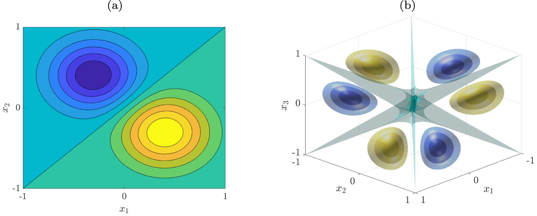
The antisymmetrized two- and three-dimensional Gaussian kernels are visualized in figure 1. The feature space mapping of the antisymmetric kernel $k_\mathrm{a}$ is the antisymmetrization operator $\mathcal{A}$ applied to the feature space mapping of the kernel k.

Example 3.4. For $\mathbb{X} \subset \mathbb{R}^2$, the feature space of the quadratic kernel $k(x, x^{\prime}) = (1 + x^\top x^{\prime})^2$ is spanned by $\{1, x_1, x_2, x_1^2, x_1 x_2, x_2^2 \}$ and thus six-dimensional. The feature space of the antisymmetrized kernel $k_\mathrm{a}$ is spanned by the two antisymmetric functions $\{x_1 - x_2, x_1^2 - x_2^2 \}$. This illustrates that the feature space is significantly reduced. $\triangle$

Zoom In Zoom Out Reset image size

Polynomial kernels of arbitrary degree p for d-dimensional spaces will be discussed in more detail in section 3.2.

Remark 3.5. The Mercer features of a kernel k are defined by the eigenfunctions of the integral operator

$$\begin{equation*} (\mathcal{T}_k f)(x) = \int k(x, x^{\prime}) f(x^{\prime}) \mathrm{d} \mu(x^{\prime}) \end{equation*}$$

multiplied by the square root of the associated eigenvalues λ, see [19]. The Mercer features of an antisymmetric kernel $k_\mathrm{a}$ are automatically antisymmetric. This can be seen as follows: let ϕ be an eigenfunction of $\mathcal{T}_{k_\mathrm{a}}$ with corresponding eigenvalue λ, then

$$\begin{equation*} \lambda \varphi(\pi(x)) = \int k_\mathrm{a}(\pi(x), x^{\prime}) \varphi(x^{\prime}) \mathrm{d} \mu(x^{\prime}) = \mathrm{sgn}(\pi) \int k_\mathrm{a}(x, x^{\prime}) \varphi(x^{\prime}) \mathrm{d} \mu(x^{\prime}) = \lambda \mathrm{sgn}(\pi) \varphi(x). \end{equation*}$$

Mercer features of the Gaussian kernel and its antisymmetric and symmetric (see section 4) counterparts—computed by a spectral decomposition of the covariance operator, cf [29]—are shown in figure 2.

Definition 3.6  We call a kernel permutation-invariant if

$$\begin{equation*} k(x, x^{\prime}) = k(\pi(x), \pi(x^{\prime})) \end{equation*}$$

for all permutations π ∈ S_d .

The Gaussian kernel and the polynomial kernel are permutation-invariant since the standard inner product and induced norm are permutation-invariant, i.e. $\left\langle{x}{x^{\prime}}\right\rangle = \left\langle{\pi(x)}{\pi(x^{\prime})}\right\rangle$ for a permutation π ∈ S_d . The antisymmetric kernel $k_\mathrm{a}$ is permutation-invariant by construction. While many kernels used in practice are naturally permutation-invariant, an open question is whether this assumption limits the expressivity of the induced function space. We will analyze the properties of the Gaussian kernel in section 3.3. The permutation-invariance allows us to simplify the representation of the antisymmetric kernel.

Lemma 3.7. Given a permutation-invariant kernel k, it holds that

$$\begin{equation*} k_\mathrm{a}(x, x^{\prime}) = \frac{1}{d!} \sum_{\pi \in S_d} \mathrm{sgn}(\pi) k\big(\pi(x), x^{\prime}\big) = \frac{1}{d!} \sum_{\pi \in S_d} \mathrm{sgn}(\pi) k\big(x, \pi(x^{\prime})\big). \end{equation*}$$

proof We obtain

$$\begin{align*} k_\mathrm{a}(x, x^{\prime}) & = \frac{1}{d!^2} \sum_{\pi \in S_d} \sum_{\pi^{\prime} \in S_d} \mathrm{sgn}(\pi) \mathrm{sgn}(\pi^{\prime}) k\big(\pi(x), \pi^{\prime}(x^{\prime})\big) \\ & = \frac{1}{d!^2} \sum_{\pi \in S_d} \sum_{\pi^{\prime} \in S_d} \mathrm{sgn}(\pi) \mathrm{sgn}(\pi^{\prime}) k\big(\left[(\pi^{\prime})^{-1} \circ \pi\right](x), x^{\prime}\big) \\ & = \frac{1}{d!^2} \sum_{\pi \in S_d} \sum_{\pi^{\prime} \in S_d} \mathrm{sgn}\big((\pi^{\prime})^{-1} \circ \pi\big) k\big(\left[(\pi^{\prime})^{-1} \circ \pi\right](x), x^{\prime}\big) \\ & = \frac{1}{d!} \sum_{\pi \in S_d} \mathrm{sgn}(\pi) k\big(\pi(x), x^{\prime}\big) \end{align*}$$

since all permutations occur d! times. In the third line, we used the same properties of permutations as above. The proof for the second representation is analogous.

For the sake of simplicity, assume now that the kernel k is permutation-invariant. We want to show that for a universal kernel k, the reproducing kernel Hilbert space induced by the corresponding antisymmetric kernel $k_\mathrm{a}$ is dense in the space of antisymmetric functions.

Proposition 3.8. Let $\mathbb{X}$ be bounded. Given a universal, permutation-invariant, continuous kernel k, the space $\mathbb{H}_a$ induced by $k_\mathrm{a}$ is dense in the space of continuous antisymmetric functions given by $C_a(\mathbb{X}) = \{f \in C(\mathbb{X}) \mid f \textrm{is antisymmetric} \}$.

proof Let f be antisymmetric. It follows that $f(x) = \mathrm{sgn}(\pi) f(\pi(x))$ for all π ∈ S_d and thus

$$\begin{equation*} f(x) = \frac{1}{d!} \sum_{\pi \in S_d} \mathrm{sgn}(\pi) f(\pi(x)). \end{equation*}$$

Since k is assumed to be universal, we can find coefficients $\alpha_i \in \mathbb{R}$ and vectors $x^{(i)} \in \mathbb{X}$ such that $||{\sum_{i = 1}^n \alpha_i k(\,\cdot\,, x^{(i)}) - f}||_\infty \lt \varepsilon$. Then

$$\begin{align*} \left\|{\sum_{i = 1}^n \alpha_i k_\mathrm{a}(\,\cdot\,, x^{(i)}) - f\,}\right\|_\infty & = \Bigg\lVert \sum_{i = 1}^n \frac{\alpha_i}{d!} \sum_{\pi \in S_d} \mathrm{sgn}(\pi) k\big(\pi(\,\cdot\,), x^{(i)}\big) - \frac{1}{d!} \sum_{\pi \in S_d} \mathrm{sgn}(\pi) f(\pi(\,\cdot\,)) \Bigg\rVert_\infty \\ & = \Bigg\lVert \frac{1}{d!} \sum_{\pi \in S_d} \mathrm{sgn}(\pi) \underbrace{\left[\sum_{i = 1}^n \alpha_i k\big(\pi(\,\cdot\,), x^{(i)}\big) - f(\pi(\,\cdot\,))\right]}_{\lt \varepsilon ~\forall \pi} \Bigg\rVert_\infty \lt \varepsilon.\end{align*}$$

Continuous antisymmetric functions can be approximated arbitrarily well by universal antisymmetric kernels such as the Gaussian kernel. Although we used the same number of data points for the approximation in the proof (i.e. n points for the expansion in terms of k and also $k_\mathrm{a}$), fewer data points are required in practice if we employ the antisymmetric kernel, see example 3.14.

Zoom In Zoom Out Reset image size

We have seen in example 3.4 that the feature space dimension of the polynomial kernel of order two for $\mathbb{X} \subset \mathbb{R}^2$ is reduced from six to two by the antisymmetrization. Let $q = (q_1, \dots, q_d) \in \mathbb{N}_0^d$ be a multi-index and $\left\lvert q \right\rvert = \sum_{i = 1}^{d} q_i$. We define $x^q = \prod_{i = 1}^d x_i^{q_i}$. For a d-dimensional state space $\mathbb{X}$, the polynomial kernel of order p is then given by

$$\begin{equation*} k(x, x^{\prime}) = (c + x^\top x^{\prime})^p = \sum_{0~\le \left\lvert q \right\rvert \le p} \left( \sqrt{a_{q}} x^q \right) \left( \sqrt{a_q} {x^{\prime}}^q \right), \end{equation*}$$

where

$$\begin{equation*} a_q = \binom{p}{q} \frac{c^{q_0}}{q_0!} \end{equation*}$$

and $q_0 = p - \left\lvert q \right\rvert$, cf [30]. The multinomial coefficients are defined by

$$\begin{equation*} \binom{p}{q} = \frac{p!}{q_1! \dots q_d!}. \end{equation*}$$

Thus, the feature space is spanned by the monomials $\big\{x^q ~\big|~ 0~\le \left\lvert q \right\rvert \le p \big\}$ and the dimension of the feature space is $n_\phi = \binom{p+d}{d}$, see, e.g. [31].

We now want to find the feature space of the corresponding antisymmetric kernel k_a . Given a multi-index q, assume that there exist two entries q_i and q_j with $q_i = q_j$. Since the transposition (i, j) leaves the multi-index (and thus x^q ) unchanged, this monomial will be eliminated by the antisymmetrization operator. It follows that the monomials must have distinct indices. In fact, the nonzero images of monomials under antisymmetrization are of the form

$$\begin{equation} f_\mu(x) = \begin{vmatrix} x_1^{\delta_1+\mu_1} & x_1^{\delta_2+\mu_2} & \dots & x_1^{\delta_d+\mu_d} \\ x_2^{\delta_1+\mu_1} & x_2^{\delta_2+\mu_2} & \dots & x_2^{\delta_d+\mu_d} \\ \vdots & \vdots & \ddots & \vdots \\ x_d^{\delta_1+\mu_1} & x_d^{\delta_2+\mu_2} & \dots & x_d^{\delta_d+\mu_d} \end{vmatrix}, \end{equation} \tag{ 2 }$$

where $\delta = (d-1, d-2, \dots, 0)$ and $\mu = (\mu_1, \dots, \mu_d)$ with $\mu_1~\geqslant \mu_2~\geq \dots \geqslant \mu_d \geqslant 0$ is a partition of a positive integer ⁷ , see [32]. The degrees of the terms of this antisymmetric polynomial are $|{\mu}| + \binom{d}{2}$. Since we need all monomials of order $0~\leqslant \left\lvert q \right\rvert \leqslant p$, we have to consider the partitions µ of $0~\leqslant p_r \leqslant p - \binom{d}{2}$.

This representation uses the fact that multi-indices corresponding to antisymmetric polynomials can be written as q = δ + µ, where δ is defined as above and µ a partition. It follows that an antisymmetric polynomial must be at least of order $\binom{d}{2}$. Equation (2) can be regarded as a Slater determinant (introduced below) for a specific set of functions. We also obtain the Vandermonde determinant (up to the sign) as a special case where µ = 0. Partition function

Definition 3.9 Let $s_\ell(n)$ be the function that counts the partitions of n into exactly $\ell$ parts.

A closed-form expressions for $s_\ell(n)$ is not known, but it can be expressed in terms of generating functions or computed using the recurrence relation

$$\begin{equation*} s_\ell(n) = s_\ell(n-\ell) + s_{\ell-1}(n-1), \end{equation*}$$

where we define $s_\ell(n) = 1$ if n = 0 and $\ell = 0$ and $s_\ell(n) = 0$ if $n \leqslant 0$ or $\ell \leqslant 0$ (but not $n = \ell = 0$), see [33] for more details about partitions and partition functions.

Lemma 3.10. The dimension of the feature space generated by the antisymmetrized polynomial kernel of order p is

$$\begin{equation*} n_{\phi_a} = \sum_{p_r = 0}^{p-\binom{d}{2}} \sum_{j = 0}^d s_j(p_r). \end{equation*}$$

proof Since $\binom{d}{2}$ of the $\left\lvert q \right\rvert$ exponents are already spoken for, we can use only the remaining $\left\lvert q \right\rvert - \binom{d}{2}$ to generate partitions µ, with $0~\leqslant \left\lvert q \right\rvert \leqslant p$. All these numbers can be decomposed into at most d parts since we have only d variables. If the number of components is smaller than d, we simply add zeros.

Example 3.11. For d = 3 and p = 6, the base case is δ = (2, 1, 0), and we can generate partitions for

$$\begin{align*} p_r = 0: &~ \mu = (0, 0, 0), && q = (2, 1, 0), \\ p_r = 1: &~ \mu = (1, 0, 0), && q = (3, 1, 0), \\ p_r = 2: &~ \mu = (2, 0, 0), (1, 1, 0), && q = (4, 1, 0), (3, 2, 0), \\ p_r = 3: &~ \mu = (3, 0, 0), (2, 1, 0), (1, 1, 1), && q = (5, 1, 0), (4, 2, 0), (3, 2, 1), \end{align*}$$

resulting in seven antisymmetric polynomials. $\triangle$

The sizes of the feature spaces of the polynomial kernels k and $k_\mathrm{a}$ for different dimensions d and degrees p are summarized in table 1. This shows that antisymmetric polynomial kernels might not be feasible for higher-dimensional problems. For d = 10, for example, the lowest degree of the monomials is already 45.

Table 1. Dimensions of the feature spaces spanned by the polynomial kernel k and its antisymmetric counterpart $k_\mathrm{a}$. Here, d is the dimension of the state space and p the degree of the polynomial kernel.

p	2		3		4		5		6		7		8
d	$n_\phi$	$n_{\phi_a}$	$n_\phi$	$n_{\phi_a}$	$n_\phi$	$n_{\phi_a}$	$n_\phi$	$n_{\phi_a}$	$n_\phi$	$n_{\phi_a}$	$n_\phi$	$n_{\phi_a}$	$n_\phi$	$n_{\phi_a}$
2	6	2	10	4	15	6	21	9	28	12	36	16	45	20
3	10	0	20	1	35	2	56	4	84	7	120	11	165	16
4	15	0	35	0	70	0	126	0	210	1	330	2	495	4

We will now analyze the properties of the Gaussian kernel. We have shown in Proposition 3.8 that the space spanned by the antisymmetric Gaussian kernel is dense in the space of continuous antisymmetric functions. For the Gaussian kernel, the expression obtained in lemma 3.7 can be simplified even further.

Lemma 3.12. Let k be the Gaussian kernel with bandwidth σ, then

$$\begin{align*} k_\mathrm{a}(x, x^{\prime}) = \frac{1}{d!} \begin{vmatrix} e^{-\frac{(x_1 - x^{\prime}_1)^2}{2\sigma^2}} & \dots & e^{-\frac{(x_1 - x^{\prime}_d)^2}{2\sigma^2}} \\ \vdots & \ddots & \vdots \\ e^{-\frac{(x_d - x^{\prime}_1)^2}{2\sigma^2}} & \dots & e^{-\frac{(x_d - x^{\prime}_d)^2}{2\sigma^2}} \\ \end{vmatrix}. \end{align*}$$

proof Applying Leibniz' formula

$$\begin{equation*} \det(A) = \sum_{\pi \in S_d} \mathrm{sgn}(\pi) \prod_{i = 1}^d a_{\pi(i), i}, \end{equation*}$$

we have

$$\begin{align*} \begin{vmatrix} e^{-\frac{(x_1 - x^{\prime}_1)^2}{2\sigma^2}} & \dots & e^{-\frac{(x_1 - x^{\prime}_d)^2}{2\sigma^2}} \\ \vdots & \ddots & \vdots \\ e^{-\frac{(x_d - x^{\prime}_1)^2}{2\sigma^2}} & \dots & e^{-\frac{(x_d - x^{\prime}_d)^2}{2\sigma^2}} \\ \end{vmatrix} & = \sum_{\pi \in S_d} \mathrm{sgn}(\pi) \prod_{i = 1}^d e^{-\frac{(x_{\pi(i)} - x^{\prime}_i)^2}{2\sigma^2}} \\ & = \sum_{\pi \in S_d} \mathrm{sgn}(\pi) e^{-\frac{\sum_{i = 1}^d (x_{\pi(i)} - x^{\prime}_i)^2}{2\sigma^2}} \\ & = \sum_{\pi \in S_d} \mathrm{sgn}(\pi) e^{-\frac{||{\pi(x) - x^{\prime}}||^2}{2\sigma^2}} \\ & = \sum_{\pi \in S_d} \mathrm{sgn}(\pi) k(\pi(x), x^{\prime}). \end{align*}$$

Lemma 3.7 then yields the desired result.

This decomposition is akin to the well-known Slater determinant (see, e.g. [34]), which defines an antisymmetric wave function by

$$\begin{equation*} \psi_\mathrm{a}(x) = \frac{1}{\sqrt{d!}} \begin{vmatrix} \psi_1(x_1) & \dots & \psi_d(x_1) \\ \vdots & \ddots & \vdots \\ \psi_1(x_d) & \dots & \psi_d(x_d) \\ \end{vmatrix}. \end{equation*}$$

Notice that here the normalization factor is chosen in such a way that, provided the wave functions ψ_i , $i = 1, \dots, d$, are normalized and orthogonal to each other, $\psi_\mathrm{a}$ is normalized as well.

Remark 3.13. We can define a more general class of antisymmetric kernels. Let $f : \mathbb{R} \to \mathbb{R}$ be a function, then

$$\begin{equation*} k_\mathrm{a}(x, x^{\prime}) = \frac{1}{d!} \begin{vmatrix} f(|{x_1 - x^{\prime}_1}|) & \dots & f(|{x_1 - x^{\prime}_d}|) \\ \vdots & \ddots & \vdots \\ f(|{x_d - x^{\prime}_1}|) & \dots & f(|{x_d - x^{\prime}_d}|) \\ \end{vmatrix} \end{equation*}$$

defines an antisymmetric kernel. We call such a function $k_\mathrm{a}$ a Slater kernel. The Gaussian kernel can be obtained by setting $f(r) = e^{-\frac{r^2}{2\sigma^2}}$ and the Laplacian kernel—using the 1-norm—by setting $f(r) = e^{-\frac{r}{\sigma}}$. Alternatively, kernels based on generalized Slater determinants could be constructed or by concatenating creation and annihilation operators, see also [11–13].

The advantage of the Slater determinant formulation is that we can compute it efficiently using matrix decomposition techniques, without having to iterate over all permutations, which would be clearly infeasible for higher-dimensional problems.

Example 3.14. In order to illustrate the difference between a standard Gaussian kernel k and its antisymmetrized counterpart $k_\mathrm{a}$, we define an antisymmetric function $f : \mathbb{R}^2~\to \mathbb{R}$ by $f(x) = \sin(\boldsymbol{\pi}(x_1 - x_2))$ and apply kernel ridge regression (see, e.g. [31]) to randomly sampled data points ⁸ . That is, we generate m data points x⁽ⁱ⁾ in $\mathbb{X} = [-1, 1] \times [-1, 1]$ and compute $y^{(i)} = f(x^{(i)})$. We then try to recover f from the training data $\big\{(x^{(i)}, y^{(i)})\big\}_{i = 1}^m$. Additionally, we define an augmented data set of size 2 m by adding the antisymmetrized data set, i.e. $\big\{(x^{(i)}, y^{(i)})\big\}_{i = 1}^m \cup \big\{(\pi(x^{(i)}), -y^{(i)}\big\}_{i = 1}^m$, where π = (1, 2) in cycle notation. The bandwidth of the kernel is set to $\sigma = \frac{1}{2}$. The results are shown in figure 3. We measure the root-mean-square error (RMSE)—averaged over 5000 runs—in the midpoints of a regular 30 × 30 box discretization of the domain. Kernel ridge regression using $k_\mathrm{a}$ results in more accurate function approximations and is, for small m, numerically equivalent to kernel ridge regression using k applied to the augmented data set of size 2 m. For larger values of m, doubling the size of the data set leads to ill-conditioned matrices and increased numerical errors ⁹ . $\triangle$

Zoom In Zoom Out Reset image size

The example shows that the antisymmetrized kernel is indeed advantageous, it enables a more accurate representation without increasing the size of the data set. For higher-dimensional problems, this effect will be even more pronounced. To obtain the same accuracy for a three-dimensional antisymmetric function, we would already need 6 m data points. The kernel evaluations, on the other hand, become more expensive, but are easily parallelizable. The bottleneck of kernel-based methods is often the size of the training data set, which enters in a cubic way (since a generally dense system of linear equations has to be solved, or, if we are interested in eigenfunctions of operators associated with dynamical systems, a generalized eigenvalue problem).

For the approximation of differential operators, we will also need partial derivatives of the kernel $k_\mathrm{a}$. Since $k_\mathrm{a}$ just comprises alternating sums of kernel functions k, we can compute derivatives of $k_\mathrm{a}$ by summing over derivatives of k. For polynomial and Gaussian kernels, the derivatives of k can be found in [25]. Alternatively, the partial derivatives of the antisymmetric Gaussian kernel can be computed via Slater determinants.

Example 3.15.  For the antisymmetric Gaussian kernel, let $K^{e_l} \in \mathbb{R}^{d \times d}$ be the matrix with entries

$$\begin{align*} K^{\,e_l}_{i j} = \begin{cases} -\frac{1}{\sigma^2} (x_i - x^{\prime}_j) e^{-\frac{(x_i - x^{\prime}_j)^2}{2\sigma^2}}, & i = l, \\ e^{-\frac{(x_i - x^{\prime}_j)^2}{2\sigma^2}}, & i \ne l. \end{cases} \end{align*}$$

Then

$$\begin{equation*} \mathcal{D}^{e_l} k_\mathrm{a}(x, x^{\prime}) = \frac{1}{d!} \det(K^{e_l}). \end{equation*}$$

Similar formulas can be derived for the second-order derivatives. $\triangle$

We call a function $f : \mathbb{X} \to \mathbb{R}$ symmetric if

$$\begin{equation*} f(x) = f(\pi(x)) \end{equation*}$$

for all permutations π ∈ S_d and define the symmetrization operator

$$\begin{equation*} (\mathcal{S} f)(x) = \frac{1}{d!} \sum_{\pi \in S_d} f(\pi(x)). \end{equation*}$$

Symmetric kernel function

Definition 4.1 Let $k : \mathbb{X} \times \mathbb{X} \to \mathbb{R}$ be a kernel. We then define a symmetric function $k_\mathrm{s} : \mathbb{X} \times \mathbb{X} \to \mathbb{R}$ by

$$\begin{equation*} k_\mathrm{s}(x, x^{\prime}) = \frac{1}{d!^2} \sum_{\pi \in S_d} \sum_{\pi^{\prime} \in S_d} k\big(\pi(x), \pi^{\prime}(x^{\prime})\big). \end{equation*}$$

We simply omitted the signs of the permutations here. As before, if $k(x, x^{\prime}) = k(x^{\prime}, x)$, then also $k_\mathrm{s}(x, x^{\prime}) = k_\mathrm{s}(x^{\prime}, x)$. The function $k_\mathrm{s}$ is permutation-symmetric in both arguments. Note that the definition of permutation-symmetry is different from permutation-invariance, which was defined by $k(x, x^{\prime}) = k(\pi(x), \pi(x^{\prime}))$. Permutation-symmetric kernels are, however, automatically permutation-invariant. We briefly restate the above results for symmetric functions, the proofs are analogous to their counterparts for antisymmetric functions.

Lemma 4.2. The function $k_\mathrm{s}$ defines an s.p.d. kernel.

Example 4.3.  For $\mathbb{X} \subset \mathbb{R}^2$, the feature space of the symmetrized polynomial kernel of order 2 is spanned by the symmetric functions $\{1, x_1 + x_2, x_1^2 + x_2^2, x_1 x_2 \}$. $\triangle$

More general results for polynomial kernels will be derived in section 4.2. Eigenfunctions of the integral operator associated with $k_\mathrm{s}$ are symmetric. Mercer features of the symmetrized Gaussian kernel for d = 2 are shown in figure 2.

Lemma 4.4. Given a permutation-invariant kernel k, it holds that

$$\begin{equation*} k_\mathrm{s}(x, x^{\prime}) = \frac{1}{d!} \sum_{\pi \in S_d} k\big(\pi(x), x^{\prime}\big) = \frac{1}{d!} \sum_{\pi \in S_d} k\big(x, \pi(x^{\prime})\big). \end{equation*}$$

Analogously, continuous symmetric functions can be approximated arbitrarily well by symmetric universal kernels.

Proposition 4.5. Let $\mathbb{X}$ be bounded. Given a universal, permutation-invariant, continuous kernel k, the space $\mathbb{H}_s$ induced by $k_\mathrm{s}$ is dense in the space of continuous symmetric functions given by $C_\mathrm{s}(\mathbb{X}) = \{f \in C(\mathbb{X}) \mid f \textrm{is symmetric} \}$.

Let us compute the dimensions of the feature spaces spanned by symmetrized polynomial kernels.

Lemma 4.6. The dimension of the feature space generated by the symmetrized polynomial kernel of order p is

$$\begin{equation*} n_{\phi_s} = \sum_{p_r = 0}^{p} \sum_{j = 0}^d s_j(p_r). \end{equation*}$$

proof Let π be a permutation, then the multi-indices q and π(q) generate the same feature space function when we apply the symmetrization operator $\mathcal{S}$ to the corresponding monomials x^q and $x^{\pi(q)}$. We thus have to consider only partitions µ of the integers $0 \leqslant \left\lvert q \right\rvert \leqslant p$ since the ordering of the multi-indices does not matter.

This case is similar to the antisymmetric case, with the difference that we require partitions of integers up to p instead of $p-\binom{d}{2}$. Table 2 lists the dimensions of the feature spaces spanned by the polynomial kernel k and its symmetric version $k_\mathrm{s}$ for different combinations of d and p. Compared to the standard polynomial kernel, the number of features is significantly lower, but higher than the number of features generated by the antisymmetric polynomial kernel.

Table 2. Dimensions of the feature spaces spanned by the polynomial kernel k and its symmetric counterpart $k_\mathrm{s}$. Here, d is again the dimension of the state space and p the degree, cf table 1.

p	2		3		4		5		6		7		8
d	$n_\phi$	$n_{\phi_s}$	$n_\phi$	$n_{\phi_s}$	$n_\phi$	$n_{\phi_s}$	$n_\phi$	$n_{\phi_s}$	$n_\phi$	$n_{\phi_s}$	$n_\phi$	$n_{\phi_s}$	$n_\phi$	$n_{\phi_s}$
2	6	4	10	6	15	9	21	12	28	16	36	20	45	25
3	10	4	20	7	35	11	56	16	84	23	120	31	165	41
4	15	4	35	7	70	12	126	18	210	27	330	38	495	53

The symmetric kernel cannot be expressed as a Slater determinant anymore, but we can utilize a related concept. The permanent of a matrix $A \in \mathbb{R}^{d \times d}$ is defined by

$$\begin{equation*} \mathrm{per}(A) = \sum_{\pi \in S_d} \prod_{i = 1}^d a_{\pi(i), i} = : \left|\begin{matrix} ^{\!\!\!\!{–}}a_{11} & \dots & a_{1d} \\ \vdots & \ddots & \vdots \\ _{\!\!\!\!{–}}a_{d1} & \dots & a_{dd} \end{matrix}\right|_{\!\!\!\!{–}}^{\!\!\!\!{–}}. \end{equation*}$$

While for d = 2 the permanent can be written as a determinant (by flipping the sign of a₁₂ or a₂₁), this is not possible anymore for $d \geqslant 3$ [35]. No polynomial-time algorithm for the computation of the permanent is known, but there are efficient approximation schemes for matrices with non-negative entries [36].

Lemma 4.7. Let k be the Gaussian kernel with bandwidth σ, then

$$\begin{equation*} k_\mathrm{s}(x, x^{\prime}) = \frac{1}{d!} \left|\begin{matrix} ^{\!\!\!\!{–}}{}e^{-\frac{(x_1 - x^{\prime}_1)^2}{2\sigma^2}} & \dots & e^{-\frac{(x_1 - x^{\prime}_d)^2}{2\sigma^2}} \\ \vdots & \ddots & \vdots \\ _{\!\!\!\!{–}}e^{-\frac{(x_d - x^{\prime}_1)^2}{2\sigma^2}} & \dots & e^{-\frac{(x_d - x^{\prime}_d)^2}{2\sigma^2}}\\ \end{matrix}\right|_{\!\!\!\!{–}}^{\!\!\!\!{–}}. \end{equation*}$$

proof The proof is analogous to the one for lemma 3.12. Using the definition of the permanent, we obtain

$$\begin{align*} \left|\begin{matrix} ^{\!\!\!\!{–}}{}e^{-\frac{(x_1 - x^{\prime}_1)^2}{2\sigma^2}} & \dots & e^{-\frac{(x_1 - x^{\prime}_d)^2}{2\sigma^2}}{}^{\!\!\!\!\!-} \\ \vdots & \ddots & \vdots \\ _{\!\!\!\!{–}}{}e^{-\frac{(x_d - x^{\prime}_1)^2}{2\sigma^2}} & \dots & e^{-\frac{(x_d - x^{\prime}_d)^2}{2\sigma^2}} \\ \end{matrix}\right|_{\!\!\!\!{–}}^{\!\!\!\!{–}} & = \sum_{\pi \in S_d} \prod_{i = 1}^d e^{-\frac{(x_{\pi(i)} - x^{\prime}_i)^2}{2\sigma^2}} \\ & = \sum_{\pi \in S_d} e^{-\frac{\sum_{i = 1}^d (x_{\pi(i)} - x^{\prime}_i)^2}{2\sigma^2}} \\ & = \sum_{\pi \in S_d} e^{-\frac{||{\pi(x) - x^{\prime}}||^2}{2\sigma^2}} \\ & = \sum_{\pi \in S_d} k(\pi(x), x^{\prime}). \end{align*}$$

The result then follows from lemma 4.4.

Example 4.8. Assume we have a set of undirected graphs that we would like to classify or categorize. The results should not depend on the vertex labels and thus be identical for isomorphic graphs. Let $A, A^{\prime} \in \mathbb{R}^{d \times d}$ be the adjacency matrices of the graphs G and $G^{\prime}$, respectively. We define a Gaussian kernel for graphs by

$$\begin{equation*} k(G, G^{\prime}) = \exp\left(-\frac{||{A-A^{\prime}}||_F^2}{2\sigma^2}\right), \end{equation*}$$

where $||{\,\cdot\,}||_F$ denotes the Frobenius norm, and make it symmetric as described above. The only difference here is that we have to define $\pi(A) = \big( a_{\pi(i),\pi(j)} \big)_{i, j = 1}^d$ to permute rows and columns simultaneously. The kernel function $k_\mathrm{s} (G, G^{\prime})$ can then be expressed in terms of so-called hyperpermanents. We have

$$\begin{equation*} k_\mathrm{s} (G, G^{\prime}) = \sum_{\pi \in S_d} \exp\left(-\frac{||{\pi(A)-A^{\prime}}||_F^2}{2\sigma^2}\right) = \sum_{\pi \in S_d} \prod_{i = 1}^d \prod_{j = 1}^d \exp\left(-\frac{\big(a_{\pi(i),\pi(j)}- a^{\prime}_{i,j}\big)^2}{2\sigma^2}\right). \end{equation*}$$

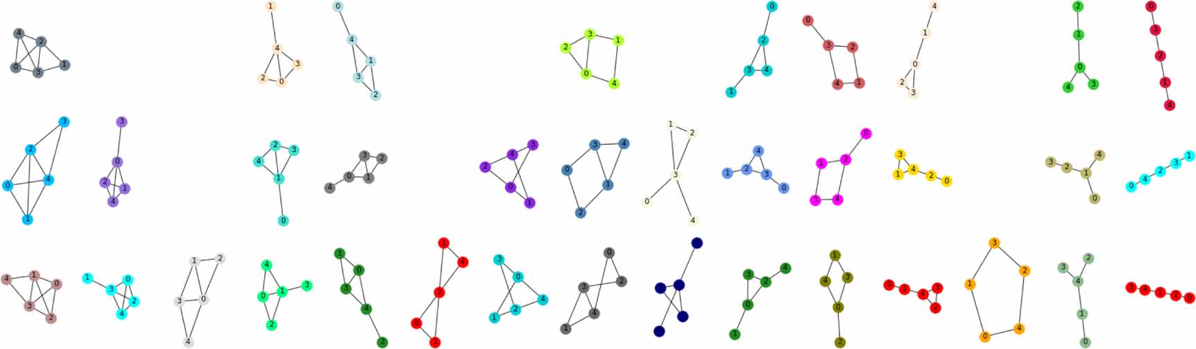
The derivation of a formula for the Laplace expansion of hyperpermanents can be found in appendix A.1. For the considered example, we set σ = 1 and randomly generate a set of 100 undirected connected graphs of size d = 5. We then apply kernel PCA, see [17], using the symmetric kernel $k_\mathrm{s}$. Sorting the graphs according to the first principal component, we obtain the ordering shown in figure 4 (only a subset of the graphs is displayed). Isomorphic graphs are grouped into the same category. $\triangle$

Zoom In Zoom Out Reset image size

Other learning algorithms such as kernel k-means, kernel ridge regression, or support vector machines can be used in the same way, enabling us to cluster, make predictions for, or classify data where the order of elements is irrelevant.

The aim now is to express a symmetric kernel not as a Slater permanent but as a product or quotient of antisymmetric functions. As shown in section 3.1, an antisymmetric kernel is zero for all x for which a (non-trivial) permutation π exists such that π(x) = x. Therefore, products of antisymmetric kernels are zero for such x as well, see also figure 5. We thus mainly restrict ourselves to quotients. Let $k_\mathrm{a}^{(1)}$ and $k_\mathrm{a}^{(2)}$ be two permutation-invariant antisymmetric kernels and $k_\mathrm{a}^{(2)}(x, x^{\prime}) \ne 0$. We define

$$\begin{equation*} k_\mathrm{s}(x, x^{\prime}) = \frac{k_\mathrm{a}^{(1)}(x, x^{\prime})}{k_\mathrm{a}^{(2)}(x, x^{\prime})}. \end{equation*}$$

Then

$$\begin{equation*} k_\mathrm{s}(\pi(x), x^{\prime}) = \frac{k_a^{(1)}(\pi(x), x^{\prime})}{k_\mathrm{a}^{(2)}(\pi(x), x^{\prime})} = \frac{\mathrm{sgn}(\pi) k_\mathrm{a}^{(1)}(x, x^{\prime})}{\mathrm{sgn}(\pi) k_\mathrm{a}^{(2)}(x, x^{\prime})} = k_\mathrm{s}(x, x^{\prime}). \end{equation*}$$

Remark 4.9. If the numerator and denominator can be written as determinants, i.e. $k_\mathrm{a}^{(1)}(x, x^{\prime}) = \det(K_1)$ and $k_\mathrm{a}^{(2)}(x, x^{\prime}) = \det(K_2)$, we obtain

$$\begin{equation*} k_\mathrm{s}(x, x^{\prime}) = \frac{\det(K_1)}{\det(K_2)} = \det(K_1) \det(K_2^{-1}) = \det(K_1~K_2^{-1}). \end{equation*}$$

Example 4.10. Suppose d = 2. Let k⁽¹⁾ and k⁽²⁾ be two Gaussian kernels with bandwidths σ₁ and σ₂, respectively, where $\sigma_1 \lt \sigma_2$. If the bandwidths are sufficiently small, either $k^{(1)}(x, x^{\prime})$ and $k^{(2)}(x, x^{\prime})$ or $k^{(1)}(\pi(x), x^{\prime})$ and $k^{(2)}(\pi(x), x^{\prime})$ will be close to zero (unless π(x) = x), where π = (1, 2) in cycle notation. Assume w.l.o.g. the latter holds, then

$$\begin{equation*} k_\mathrm{s}(x, x^{\prime}) = \frac{k_\mathrm{a}^{(1)}(x, x^{\prime})}{k_\mathrm{a}^{(2)}(x, x^{\prime})} = \frac{k^{(1)}(x, x^{\prime}) - k^{(1)}(\pi(x), x^{\prime})}{k^{(2)}(x, x^{\prime}) - k^{(2)}(\pi(x), x^{\prime})} \approx \frac{k^{(1)}(x, x^{\prime})}{k^{(2)}(x, x^{\prime})}, \end{equation*}$$

which is a Gaussian with bandwidth σ satisfying $\frac{1}{\sigma^2} = \frac{1}{\sigma_1^2} - \frac{1}{\sigma_2^2}$. This is illustrated in figure 5. Furthermore, the limit of $k_\mathrm{s}(x,x^{\prime})$ as $x_2~\rightarrow x_1$ exists and is given by

$$\begin{equation*} k_\mathrm{s}(x, x^{\prime}) = \frac{\sigma_2^2}{\sigma_2^1} \frac{k^{(1)}(x, x^{\prime})}{k^{(2)}(x, x^{\prime})}, \end{equation*}$$

with $x = [x_1, x_1]^\top$, see appendix B. $\triangle$

Zoom In Zoom Out Reset image size

The symmetric Gaussian kernel can be approximated by a quotient of antisymmetric Gaussian kernels, which can be evaluated in $\mathcal{O}(d^3)$, thus avoiding the non-polynomial complexity of the permanent. The question whether such kernels are universal is beyond the scope of this work.

Let us first consider a simple one-dimensional two-particle system. We define a potential V by

$$\begin{equation*} V(x) = \begin{cases} 0, & 0~\leqslant x \leqslant L, \\ \infty, & \textrm{otherwise}. \end{cases} \end{equation*}$$

Furthermore, we assume that the two particles do not interact and obtain the Schrödinger equation

$$\begin{equation} -\frac{\hbar^2}{2~\mathbf{m}} \Delta \psi(x_1, x_2) = E \psi(x_1, x_2) \end{equation} \tag{ 3 }$$

for $0 \leqslant x_1, x_2 \leqslant L$. By separating the two variables, we obtain the classical particle in a box problem, with eigenvalues $E_\ell = \frac{\hbar^2~\pi^2~\ell^2}{2~\mathbf{m} L^2}$ and eigenfunctions $\psi_\ell(x) = \sqrt{\frac{2}{L}} \sin\left( \frac{\pi \ell x}{L} \right)$, for $\ell = 1, 2, 3, \dots$, see, for instance, [37]. For the two-particle system, the eigenvalues are hence of the form

$$\begin{equation*} E_{\ell_1, \ell_2} = E_{\ell_1} + E_{\ell_2} = \frac{\hbar^2~\pi^2 (\ell_1^2 + \ell_2^2)}{2~\mathbf{m} L^2} \end{equation*}$$

and the eigenfunctions are

$$\begin{equation*} \psi_{\ell_1, \ell_2}(x_1, x_2) = \psi_{\ell_1}(x_1) \psi_{\ell_2}(x_2) = \frac{2}{L} \sin\left( \frac{\pi \ell_1 x_1}{L} \right) \sin\left( \frac{\pi \ell_2 x_2}{L} \right). \end{equation*}$$

However, since the two particles are physically indistinguishable, the wave functions must satisfy $|{\psi_{\ell_1, \ell_2}(x_1, x_2)|}^2 = |{\psi_{\ell_1, \ell_2}(x_2, x_1)}|^2$, which implies that the functions are either symmetric (if the particles are bosons) or antisymmetric (if the particles are fermions). Let us assume that the two particles are electrons, i.e. fermions. We thus want to compute antisymmetric solutions of the time-independent Schrödinger equation by applying the approach introduced in section 2.2, see also [25]. In the same way, we could assume that the particles are bosons and compute symmetric solutions by replacing the antisymmetric kernel by a symmetric kernel.

We define ћ = 1, $\mathbf{m} = 1$, and $L = \boldsymbol{\pi}$, choose the antisymmetric Gaussian kernel with bandwidth σ = 0.1, and generate m = 900 uniformly sampled points in [0, L]×[0, L]. Additionally, to ensure that the eigenfunctions are zero outside the box, we place 124 equidistantly distributed test points on the boundary and enforce $\psi_{\ell_1, \ell_2}(x_1, x_2) = 0$ for these boundary points. We thus have to solve a constrained eigenvalue problem and use the algorithm described in [38]. The first three eigenfunctions ψ_1,2, ψ_1,3, and ψ_2,3 are shown in figure 6 and good approximations of the analytically computed eigenfunctions. The probability that the two electrons are in the same location is always zero. Furthermore, the results show that by increasing the number of data points we obtain more accurate and less noisy estimates of the true eigenvalues.

Remark 5.1.  We would like to point out that

• This example is just meant as an illustration of the concepts and not as a realistic physical model;
• Eigenfunctions with $\ell_1 = \ell_2$ are symmetric and eliminated by the antisymmetrization operation;
• Approximations of the eigenfunctions can be obtained using far fewer points ($m \lt 50$), but the eigenvalues will be considerably overestimated (kernels tailored to quantum mechanics applications might lead to better approximations);
• The antisymmetry assumption is encoded only in the kernel, not in the Schrödinger equation itself.

Zoom In Zoom Out Reset image size

This can be easily extended to the multi-particle case. We now add electron–electron interaction terms resulting in the Hamiltonian

$$\begin{equation*} \mathcal{H} = -\frac{\hbar^2}{2~\mathbf{m}} \Delta + \sum_{i \ne j} \frac{1}{|{x_i - x_j}|}. \end{equation*}$$

For d = 3, we randomly generate 3000 interior points and 600 boundary points to enforce Dirichlet boundary conditions. We choose a Gaussian kernel with bandwidth σ = 0.1, assemble the Gram matrices, and again solve the resulting constrained eigenvalue problem. The results are shown in figure 7. For the sake of comparison, we also plot the corresponding eigenfunctions of the Schrödinger equation without the electron–electron interaction. It can be seen that the eigenfunctions for the separable case are similar to the eigenfunctions where the interaction terms are included. For this particular system, the interaction terms do not seem to have a drastic effect on the system's low-lying energy states. In general, however, their effect on the electronic wavefunction can be significant. We also remark that energies and wavefunctions of the interacting system could in principle be approximated by perturbation techniques. However, due to the degeneracy of the antisymmetric states, such a perturbation analysis seems beyond the scope of this work.

Zoom In Zoom Out Reset image size

As a second example, we consider a data set of acyclic molecules [39]. The aim is to determine the boiling points of these molecules containing the elements C, H, O, and S. The data set ¹⁰ consists of 183 graphs G = (V, E) representing the molecular structures and the corresponding boiling points in degrees Celsius, see figure 8 for a few examples of molecules included in the data set. The number of vertices $\left\lvert V \right\rvert$ varies between 3 and 11, where the hydrogen atoms of the molecules are neglected. Thus, in order to compare the graphs of different sizes, we expand all adjacency matrices to $\mathbb{R}^{d \times d}$ with d = 11 by appending rows and columns of zeros, representing artificial isolated nodes.

Zoom In Zoom Out Reset image size

We define a symmetrized Laplacian kernel on graphs, cf example 4.8. Given the adjacency matrices $A, A^{\prime} \in \mathbb{R}^{d \times d}$ of the graphs G = (V, E) and $G^{\prime} = (V^{\prime}, E^{\prime})$ as well as the kernel parameter $\sigma\gt0$, we define the tensor $T \in \mathbb{R}^{d \times d \times d \times d}$ by

$$\begin{equation*} t_{i,j,k,l} = \exp \left( - \frac{|{a_{i,j} - a^{\prime}_{k,l}| }}{\sigma}\right) \end{equation*}$$

for i ≠ j and k ≠ l and

$$\begin{equation*} t_{i,i,k,k} = \begin{cases} 1,& \textrm{if}\,V_i \text{ and } V^{\prime}_k\,\textrm{represent the same atom,} \\ \exp \left( - 1/\sigma \right), & \textrm{otherwise.} \end{cases} \end{equation*}$$

The latter definition ensures that we avoid unwanted effects of any ordinal labeling of the nodes. Using the hyperpermanent of T, the kernel evaluation $k_\mathrm{s}(G,G^{\prime})$ can be written as

$$\begin{equation} k_\mathrm{s}(G,G^{\prime}) = \mathrm{hper}(T) = \sum_{\pi \in S_d} \prod_{i = 1}^d \prod_{j = 1}^d t_{i, j, \pi(i), \pi(j)}. \end{equation} \tag{ 4 }$$

Note that we do not consider entries t_i,j,k,l with either i = j, k ≠ l or i ≠ j, k = l since $i = j \Leftrightarrow \pi(i) = \pi(j)$. We refer to appendix A for different methods and simplifications for computing the hyperpermanent of T.

For kernel-based (ridge) regression (see, e.g. [40]), we extract 165 adjacency matrices (≈90%) and their corresponding boiling point temperatures from the data set as training samples, the other data pairs constitute the test set. That is, for any G in the test set, the regression function is given by $f(G) = \Theta^\top K_{\textrm{train},G}$, where the vector $K_{\textrm{train}, G} \in \mathbb{R}^{165}$ is the Gram matrix (or kernel matrix) corresponding to the training samples (rows) and the test sample G (column). The vector $\Theta \in \mathbb{R}^{165}$ is the solution of $K_{\textrm{train},\textrm{train}} \Theta = b$ with b being the vector of boiling points of the molecules in the training set. We then compute the average error as well the root-mean-square error in the boiling points of the test set in order to evaluate the generalizabilty of the learned regression function. We repeat each experiment 10 000 times with randomly chosen training and test sets, the results for different kernel parameters σ are shown in figure 9(a).

Zoom In Zoom Out Reset image size

The best results in terms of the average and the root-mean-square error are obtained for kernel parameters σ between 2.5 and 2.8, see table 3 for details. According to the data set's website, the best results so far for the boiling point prediction on 90% of the set as training data and 10% as test data are achieved by applying so-called treelet kernels which exploit all possible graph/tree patterns up to a given size [39]. In this case, the average error is listed as 4.87 and the root-mean-square error as 6.75. Both values are comparable with our results.

As shown in figure 9(b), the entries of the Gram matrix tend to decrease for larger molecules. This effect can be explained by the expansion of the adjacency matrices and similarities of the molecules with small numbers of atoms. For instance, the first two compounds in the (ordered) data set are dimethyl ether (C₂H₆O) and dimethyl sulfide (C₂H₆S). Due to the expansion from $\left\lvert V \right\rvert = 3$ to $\left\lvert V \right\rvert = 11$, the majority of the permutations in (4) do not affect the adjacency matrix of $G^{\prime}$, cf appendix A.3. The block structure of the matrix arises from the ordering of the data set, i.e. each group of molecules with the same number of atoms is divided into subgroups of compounds containing one oxygen atom, two oxygen atoms, one sulfur atom, and two sulfur atoms.

Define $T^{(\mu)} \in \mathbb{R}^{d^{\times 4}}$ by

$$\begin{equation*} t^{(\mu)}_{i,j,k,l} = \begin{cases} t_{i,j,k,l} \cdot t_{i,1,k,\mu} \cdot t_{1,j,\mu,l}, & \textrm{if } i = j \textrm{ and } k = l,\\ t_{i,j,k,l}, & \textrm{otherwise.} \end{cases} \end{equation*}$$

Let $\widehat{T}^{(\mu)} \in \mathbb{R}^{(d-1)^{\times 4}}$ denote the tensor that results from $T^{(\mu)}$ by removing all entries $t^{(\mu)}_{i,j,k,l}$ with i = 1, j = 1, k = µ, or l = µ. The hyperpermanent can then be written as

$$\begin{align*} \mathrm{hper}(T) & = \sum_{\pi \in S_d} \prod_{i = 1}^d \prod_{j = 1}^d t_{i, j, \pi(i), \pi(j)}\\ & = \sum_{\pi \in S_d} t_{1, 1, \pi(1), \pi(1)} \prod_{i = 2}^d t_{i, 1, \pi(i), \pi(1)} \prod_{j = 2}^d t_{1,j,\pi(1),\pi(j)} \prod_{i = 2}^d \prod_{j = 2}^d t_{i, j, \pi(i), \pi(j)} \\ & = \sum_{\mu = 1}^d t_{1, 1, \mu, \mu} \sum_{\substack{\pi \in S_d\\ \pi(1) = \mu} } \prod_{i = 2}^d \prod_{j = 2}^d t_{i, j ,\pi(i), \pi(j)} \left ( t_{i, 1, \pi(i), \mu} t_{1,j,\mu,\pi(j)} \right )^{\delta_{ij}}\\ & = \sum_{\mu = 1}^d t_{1, 1, \mu, \mu} \mathrm{hper} \left(\widehat{T}^{(\mu)} \right), \end{align*}$$

where δ_ij denotes the Kronecker delta. Note that i = j implies π(i) = π(j).

Suppose $t_{i,j,k,l} = t_{j,i,k,l}$ and $t_{i,j,k,l} = t_{i,j,l,k}$ for all $i,j,k,l \in \{1, \dots, d\}$. For instance, this is the case for tensors T containing elementwise evaluations of Gaussian and Laplacian kernels as given in (5) and (6), respectively. The hyperpermanent of T can then be written as

$$\begin{equation} \begin{split} \mathrm{hper}(T) & = \sum_{\pi \in S_d} \prod_{i = 1}^d \prod_{j = 1}^d t_{i, j, \pi(i), \pi(j)}\\ & = \sum_{\pi \in S_d} \prod_{i = 1}^d \left( t_{i, i, \pi(i), \pi(i)} \prod_{\substack{j = 1 \\ j \neq i}}^d t_{i, j, \pi(i), \pi(j)} \right)\\ & = \sum_{\pi \in S_d} \left( \prod_{i = 1}^d t_{i, i, \pi(i), \pi(i)} \right) \left( \prod_{i = 1}^d \prod_{\substack{j = 1 \\ j \neq i}}^d t_{i, j, \pi(i), \pi(j)} \right)\\ & = \sum_{\pi \in S_d} \left( \prod_{i = 1}^d t_{i, i, \pi(i), \pi(i)} \right) \left(\prod_{i = 1}^d \prod_{j = i+1}^d t_{i, j, \pi(i), \pi(j)}^2~\right)\\ & = \sum_{\pi \in S_d} \frac{\prod_{i = 1}^d \prod_{j = i}^d t_{i, j, \pi(i), \pi(j)} ^2}{\prod_{i = 1}^d t_{i, i, \pi(i), \pi(i)}}. \end{split} \end{equation} \tag{ 7 }$$

The advantage of the above formula is that we can reduce the computational costs for the hyperpermanent. Additionally, we do not have to compute all elements of T, which also reduces the computational costs.

In order to compare graphs of different sizes, we include artificial isolated nodes in section 5.2. That is, the adjacency matrix of a given graph is expanded by adding zero entries. In this case, all permutations among the isolated nodes do not change the result of the product $\prod_{i = 1}^d \prod_{j = 1}^d t_{i, j, \pi(i), \pi(j)}$. Assume that the dimension of the adjacency matrix A used in (5) and (6) is initially $d^{\prime} \lt d$ before the expansion to $R^{d \times d}$. Then, it holds that

$$\begin{equation*} t_{i,j,\pi(i), \pi(j)} = t_{d^{\prime}+1, d^{\prime} +1, \pi(i), \pi(j)}, \end{equation*}$$

if $i\gt d^{\prime}$ or $j\gt d^{\prime}$. Thus, given two permutations π₁ and π₂ with

$$\begin{equation*} \pi_1(i) = \pi_2(i) \textrm{ for } 1\leqslant i \leqslant d^{\prime}, \end{equation*}$$

it follows that

$$\begin{equation*} \frac{\prod_{i = 1}^d \prod_{j = i}^d t_{i, j, \pi_1(i), \pi_1(j)} ^2}{\prod_{i = 1}^d t_{i, i, \pi_1(i), \pi_1(i)}} = \frac{\prod_{i = 1}^d \prod_{j = i}^d t_{i, j, \pi_2(i), \pi_2(j)} ^2}{\prod_{i = 1}^d t_{i, i, \pi_2(i), \pi_2(i)}}. \end{equation*}$$

This means that for each permutation π ∈ S_d , any of the $(d-d^{\prime})!$ permutations of the set ${\{\pi(d^{\prime}+1), \dots, \pi(d)\}}$ does not change the value of the quotient in (7). This fact can be exploited using the formula

$$\begin{align*} \mathrm{hper}(T) = \sum_{\pi \in S_d} \pi(d^{\prime}+1) \lt \dots \lt \pi(d) (d-d^{\prime})! \, \frac{\prod_{i = 1}^d \prod_{j = i}^d t_{i, j, \pi(i), \pi(j)} ^2}{\prod_{i = 1}^d t_{i, i, \pi(i), \pi(i)}}, \end{align*}$$

which enables us to decrease the number of considered permutations significantly if $d^{\prime}$ is much smaller than d.