
Abstract
The spatiotemporal dynamics of excitable media may exhibit chaotic transients. We investigate this transient chaos in the 2D Fenton–Karma model describing the propagation of electrical excitation waves in cardiac tissue and compute the average duration of chaotic transients in dependence on model parameter values. Furthermore, other characteristics like the dominant frequency, the size of the excitable gap, pseudo ECGs, the number of phase singularities and parameters characterizing the action potential duration restitution curve are determined and it is shown that these quantities can be used to predict the average transient time using polynomial regression.
Export citation and abstract BibTeX RIS

Original content from this work may be used under the terms of the Creative Commons Attribution 4.0 licence. Any further distribution of this work must maintain attribution to the author(s) and the title of the work, journal citation and DOI.
1. Introduction
Not all chaotic dynamics observed in simulations or experiments are persistent. Instead of a chaotic attractor, the dynamical system may possess a chaotic saddle in state space, an invariant set that acts like a maze in which a trajectory may be trapped for a long time until it finally finds its way to some nearby attractor. During this itinerary, the dynamics exhibits all attributes of deterministic chaos, and therefore this phenomenon is called transient chaos [1]. Chaotic transients have been observed, for example, in plankton blooms [2], neural networks [3, 4], turbulence [5], NMR-lasers [6], coupled FitzHugh–Nagumo oscillators [7], ecology [8, 9], population dynamics [10] and chimera states [11, 12]. In many spatially extended systems, the duration of transients typically increases exponentially with system size [1, 13].
An important class of systems showing spatiotemporal chaos constitute excitable media. Complex dynamics in extended excitable media may be observed in chemical reactions [14, 15], as well as neural [16] and cardiac tissue [13, 17–20]. In cardiac tissue, complex spatiotemporal dynamics is associated with cardiac arrhythmias such as ventricular fibrillation (VF). During VF, coherent mechanical contraction of the heart muscle is considerably impaired, resulting in a loss of pumping function and drop in the oxygen supply of organs, in particular the brain. VF is immediately life-threatening and requires cardiac defibrillation using high-energy electric shocks. Defibrillation, however, may have severe side effects including intolerable pain [21, 22], tissue damage [23, 24], and worsening of prognosis [25, 26] indicating a significant medical need. In order to develop alternate approaches, the mechanisms underlying the onset and termination [27, 28] of cardiac arrhythmias need to be understood in more detail. In this context it is remarkable, that self-terminations of cardiac arrhythmias have been reported in clinical studies [29–31], although the underlying mechanisms remain elusive. Self-termination of spatiotemporal chaos has also been observed in numerical simulations of cardiac tissue [13, 20, 32] and in experiments using Langendorff-perfused intact rabbit and pig hearts. Conditions for the onset and termination of atrial and ventricular fibrillation and the impact of pharmaceutical interventions have been discussed by Qu and Weiss [33] and recently a biological mechanism for terminating atrial fibrillation has been identified based on an additional ion channel that is activated by the arrhythmia [34, 35].
Since in patients, the length of a chaotic transient phase (i.e., the duration of the life-threatening arrhythmic episode) is crucial, we address in this paper as a first step to better cope with transients in practice the question, whether we can predict the average transient time based on observable features of the (chaotic) spatiotemporal dynamics. As an example, we investigate the spiral wave dynamics occurring with the Fenton–Karma model that will be introduced in section 2. Transient chaos in this model and a method for quantifying the (average) transient time are discussed in section 3. In section 4 we introduce features that characterize the spatiotemporal dynamics of the Fenton–Karma model. These characteristic quantities are used in section 5 to predict the length of the chaotic transients for different model parameters. Our results are summarized and discussed in section 6.
2. The Fenton–Karma model
In this study, we investigate transient chaotic dynamics in the Fenton–Karma model [13, 17, 36]. The Fenton–Karma model is a minimal, generic model for the electrophysiology of ventricular myocytes. It has three dimensionless state variables: the transmembrane voltage u and two gating variables (v, w), whose dynamics is given by


where D is the diffusion tensor, Cm the membrane capacitance, and Θ the Heaviside step function. Here, we assume the medium to be homogeneous and isotropic, and D is thus a scalar. One of the gating time-constants in the governing equation (2) for v,  , is effectively split in two to allow for an accurate reproduction of the conduction velocity restitution curve [36]:

The Fenton–Karma model represents the total transmembrane current Itot as the sum of three cumulative transmembrane currents, i.e., the slow inward current Isi, the fast inward current Ifi, the slow outward current Iso, and the external stimulation current Istim:


The reference parameter set of the Fenton–Karma model used in this study is given in table 1. Figure 1 shows a snapshot of the membrane voltage u showing unstable spiral waves.
Table 1. The parameters of the Fenton–Karma model (equations (1)–(3)) used in this study.
| Parameter | Value | Parameter | Value |
|---|---|---|---|
| D | 0.5 mm2 ms−1 |

| 13.03 ms |

| 19.6 ms |

| 1250 ms |

| 800 ms |

| 40 ms |
| τd | 0.45 ms | τ0 | 12.5 ms |
| τr | 28 ms | τsi | 29 ms |
| k | 10 |

| 0.85 |
| uc | 0.13 | uv | 0.04 |
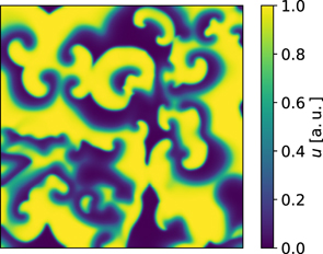
Figure 1. Spatiotemporal chaos of the Fenton–Karma model (equations (1)–(3)) using the parameters given in table 1.
Download figure:
Standard image High-resolution imageNumerically, we implemented the integration of the Fenton–Karma model on a grid of 256 × 256 cells with a uniform cell length of h = 1.0 mm. To carry out the integration, we chose the explicit Euler scheme for the voltage u and the Rush–Larsen scheme for the gating variables (v, w) with a temporal resolution of Δt = 0.1 ms. Both schemes are explicit first-order algorithms, making the calculations straightforward and cost-efficient as each step can be computed directly from the previous one.
Initial conditions were generated from a reference initial condition using random local perturbations through the stimulation current Istim. These perturbations were local in the sense that a random number of non-overlapping 5 × 5-cell regions were selected to convey a stimulation current for a fixed period of time (2 ms) within a given perturbation. The total number of perturbations, the temporal recovery intervals separating them, and the amplitudes of the respective stimulations were randomized.
3. Transient chaos in the Fenton–Karma model
The Fenton–Karma model shows transient behavior in its chaotic dynamics, i.e., any given chaotic initial condition will sooner or later converge to the stable steady state of the system 6 . The characteristic timescale of this process is called the transient time, and depends on the model parameter values and the initial conditions. The average transient time for a given set of model parameters is obtained as follows: we start with N0 = 100 initial conditions obtained by perturbing a chaotic trajectory, which all result in initially chaotic time evolutions. Then each trajectory is integrated in time until either the system has reached the steady state or a maximum integration time has been reached (105 s). As a criterion for reaching the steady state (such that the chaotic transient is terminated) we use that the variable u representing the membrane potential is smaller than 0.05 for all 256 × 256 grid points, because in this case no further excitation waves can occur.
The time series N(t) is the number of (initially chaotic) trajectories not yet in steady state at time t, where N(0) = N0. Similar to many other extended systems exhibiting transient chaos for the Fenton–Karma model, N(t) follows an exponential decay of the form f(t) = α exp(−t/τ), where α ≈ N0 is a scaling coefficient and τ is the average transient time. The average transient time and the scaling coefficient are obtained by fitting f(t) to the simulated time series N(t), as illustrated in figure 2 using the non-linear least-squares Levenberg–Marquardt algorithm as implemented in the SciPy python library (function scipy.optimize.curve_fit).
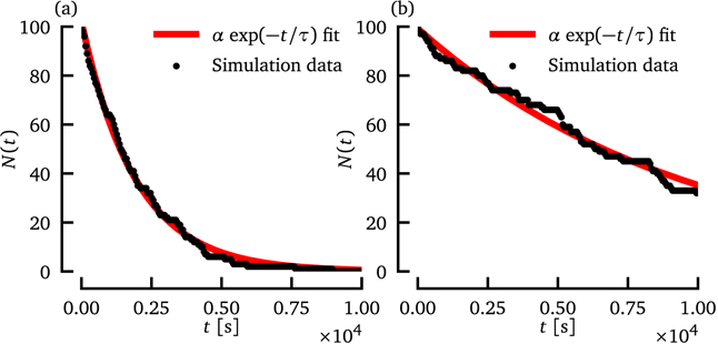
Figure 2. The number of initial conditions, which still show chaotic behavior at time t is shown for the reference parameter set (a) which is given in table 1 and for a system with varied parameters (b) (τd = 0.483 75 (+7.5%) and  (−10%)).
Download figure:
Standard image High-resolution imageTo investigate how the transient time depends on model parameters we subdivided the model parameters given in table 1 into groups of two. For every such pair, we varied each parameter independently by relative offsets ranging from −10% to +10% in steps of 2.5% (9 values in total) until all 81 combinations were exhausted. We measured the average transient time for all these combinations to arrive at the heat map representations shown in figure 3. Because some parameters led to unstable solutions under these offsets, we chose to discard them for the purpose of pairing. The remaining (stable) pairs were  , (τ0, uc
),
, (τ0, uc
),  , and
, and  . Along with the transient times we also computed several features of the chaotic dynamics that will be presented in the next section.
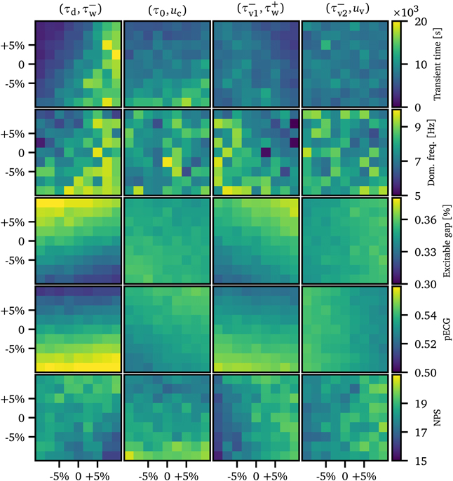
Figure 3. Average transient times and dynamical features vs parameters of the Fenton–Karma model. In each column, two model parameters were varied (±10%). In the first row, the average transient time is shown (as discussed in section 4) and in the second, third, fourth, and fifth row, the predictor values (dominant frequency, EG, pseudo ECG, and the NPS) are shown, respectively.
Download figure:
Standard image High-resolution image4. Features characterizing complex dynamics in excitable media
In the following we describe the features we extracted from the spiral wave dynamics which are used later on in section 5 for the prediction of the average transient lifetime of the system.
APD restitution curve: the APD (action-potential duration) restitution curve is an important characteristic of the dynamical behavior of the model. The duration of the action potentials is generally a function of the excitability of the tissue at the time of the stimulus. As the tissue undergoes repolarization following an action potential, excitability steadily increases until full excitability is restored. The time interval between such a completed action potential and a consecutive stimulus is called the diastolic interval (DI), and the functional relationship between it and the resulting APD of the next stimulus is summarized in the APD restitution curve as shown in figure 4(a).

Figure 4. Examples of different features, which were used to predict the average transient lifetime. In subplot (a), an exemplary APD restitution curve is shown (for parameters shown in table 1). The nonlinear regression of the restitution curve (regarding equation (9)) is depicted in red. In (b) and (c), an exemplary snapshot of the membrane potential is shown. The excitable gap (EG) (area where the membrane voltage is below ucrit) is marked in subplot (b) with shaded regions framed with white dashed lines. In subplot (c), locations of phase singularities (determined by equations (10) and (11)) are marked with white dots.
Download figure:
Standard image High-resolution imageWe determined the restitution curve analyzing the propagation of excitation pulses on a strip consisting of 16 × 2048 grid points. As a first step ten local stimuli with a fixed frequency (2 Hz) were given. After the last pulse of this sequence, another stimulus was applied with a certain temporal distance DI to the previous ones and the resulting APD was recorded. Note that there is a smallest temporal distance, which still allows the formation of an action potential. For a parametrization of the restitution curve, we performed a nonlinear least squared fit using the ansatz

An exemplary fit is shown in figure 4(a) and the fit parameters a, b, c, d, e are used in the following as potential descriptors of the dynamics entering the prediction of the average transient time.
Excitable gap (EG): the EG is defined as the area in cardiac tissue that is not excited and not refractory, i.e., where a stimulus current results in a local excitation. It is typically located between the tail of a re-entrant wave and the head of the preceding wavefront, and it can be computed as the ratio of unit cells (pixels) with membrane voltages below the system's excitation threshold ucrit and the total number of cells, 256 × 256. For our simulations with the Fenton–Karma model, we determined ucrit = 0.1a.u. by locally stimulating the system in its resting state with different amplitudes. Since stimulating a system at its resting state may require lower perturbation amplitudes compared to cases where a system (region) just recovered from a refractory period our approach to define ucrit may slightly underestimate the size of the EG in chaotically evolving systems. A typical snapshot of the EG is shown in figure 4(b). The size of the EG fluctuates in time and its temporal mean value is used in the following as a predictor for the average length of chaotic transients.
The temporal mean value of the EG (and other characteristic quantities discussed below) has been computed using 10 different trajectories representing chaotic transients each longer than 25 s. During the first 15 s these trajectories were sampled with 60 snapshots of the system per second that form the basis of the computations of the averaged quantities of interest (e.g. NPS, EG, pECG, etc). So in total the mean EG was computed on the basis of  values.
Pseudo-electrocardiogram (pECG): the pECG is the average membrane voltage across the domain with equally weighting contributions from different locations. This approach is inspired by ECGs seen in medical applications where the overall electric activity in the heart is measured through an arrangement of electrodes. Here we use the temporal average of the pseudo-ECG as a potential predictor of the mean length of transients using the same averaging procedure as in the case of the EG.
Number of phase singularities (NPS): a phase singularity (PS) is associated with the core of a rotating wave. Due to wave collision and wave breakup PS are created and annihilated resulting in temporal fluctuations of the NPS whose temporal average NPS is used as a potential predictor of transients' durations. To compute phase singularities we select the dynamical variables (u, v) of the Fenton–Karma model along with reference values (u0, v0) = (0.2, 0.2) such that, for a typical evolution of the system, the path of the projection (u, v) at any point in the domain revolves about this reference point in a circular fashion over time. This motion can be described in polar coordinates with an angle θ

which yields a matrix of angles θij (t) when applied to each spatial grid point (xi , yj ). We then evaluated the path integral

along closed paths  constituting the boundaries of small domains
  consisting of 3 × 3 pixels (grid cells). This integral attains the value ni
= ±1 if in the domain
consisting of 3 × 3 pixels (grid cells). This integral attains the value ni
= ±1 if in the domain  a clockwise or counterclockwise PS is located. Figure 4(c) shows a snapshot of the spatio-temporal wave pattern with PS represented by white dots. Temporal averaging was performed in the same way as for EG and pECG.
Dominant frequency: we extracted the most dominant frequency, which is present during the chaotic spiral wave dynamics. For this purpose, for each parameter set an episode of 10 s was considered. For each grid point on the spatial 256 × 256 domain the power spectrum was computed, the spectra from all grid points were averaged, and the frequency with the largest amplitude in the mean spectrum was considered as the dominant frequency that is used for predicting the average transient lifetime (figure 3).

Figure 5. Continuation of figure 3, the remaining feature variables (parameters a, b, c, d, and e related to the restitution curve (equation (9)) are shown for systems of different model parameters.
Download figure:
Standard image High-resolution image5. Prediction of transient duration
To predict the average transient lifetime of the system, based on the features described in the previous section we performed linear regression with polynomials of different degree. The features extracted from the spatiotemporal dynamics shown in figures 3 and 5 were used as predictors for the model. With all four combinations of parameters of the Fenton–Karma model and their variations (±10%) the data set contains 9 × 9 × 4 = 324 data points. We used a 5-fold cross validation approach (80% for training and 20% for testing) and computed the generalization (test) error as a mean over all five test sets. In order to identify the most relevant features for the fit, we computed the generalization (test) error for all combinations of predictor variables (from one to five input variables). Figure 6 shows an overview over an exemplary regression procedure for a polynomial of 2nd order and four predictor variables (NPS, b, c, e). Note, that with the degree of the polynomial we denote here the maximal degree related to a specific feature variable. Thus, when allowing cross terms, we consider the (exemplary) polynomial β × NPS2 × EG2 as a degree of second order (where β is the parameter to optimize). The first row of figure 6 shows color coded the average transient times obtained with all four model parameter combinations investigated (constituting the columns of figure 6). In the second row transient times as predicted using a polynomial of degree two are shown based on the NPS and the parameters b, c, and e characterizing the restitution curve. An example for the separation of the raw data (first row) into training data (used to estimate the coefficients of the polynomial regression) and test data (used to evaluate the performance of the polynomial regression model) is shown in rows three and four of figure 6, respectively. As pointed out above five different random splits into training and test data were performed and combined for evaluation of the regression ansatz chosen. The last row of figure 6 shows color coded the prediction error for the particular regression presented in this figure.

Figure 6. Example of the regression applied to the input data using polynomial of degree two. As input, four variables were chosen here: the NPS, and the parameters b, c, and e from the restitution curve regression (equation (9)). Interaction terms between different input variables were included. In the first row, the normalized distributions of average transient lifetimes are shown for all four variations of parameters, as discussed in section 5. After training the average transient lifetime was predicted (second row), whereas in the third and the fourth row, the prediction is divided into data points which were used for training (third row) and for testing (fourth row). The difference between the true distribution of the average transient lifetime and the prediction is depicted in the last row.
Download figure:
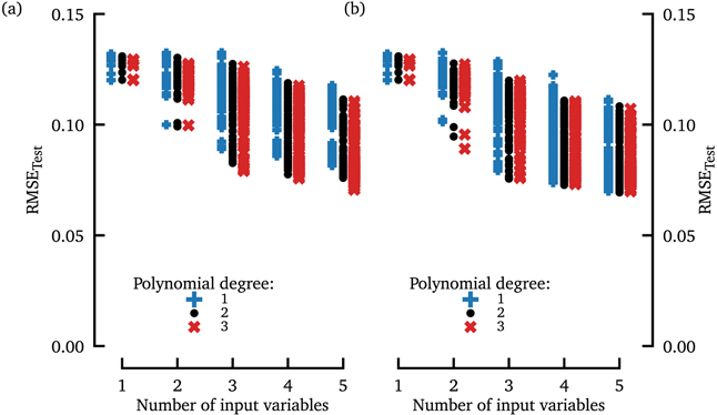
Standard image High-resolution imageAn overview of the generalization (test) error for all combinations of input variables, for 1st, 2nd, and 3rd order polynomials (with and without interaction terms between different predictors) is presented in figure 7 and tables 2–4 showing rankings of the combinations of features which provided the prediction of the transient times with polynomials of different degrees. To clarify the meaning of the obtained results, we demonstrate as an example, how the data points in the first column of figure 7(a) are computed. This first column shows the RMSETest for the case of a single (feature) input variable. Since we use nine different feature variables (NPS, pECG, EG, ...) for the prediction of the average transient lifetime, we compute nine different data points, which relate to the regression procedure based on each feature variable. The feature variable which leads to the lowest RMSETest is then given explicitly in tables 2–4. Then, in the second column (with two input variables), two feature variables were used for regression, resulting in 36 combinations of tuples consisting of two feature variables. An interesting observation in tables 2–4 is that features which provide optimal results when used alone for the prediction (dominant frequency for polynomials of degree 1 or 2, and EG with polynomials of 3rd degree) turn out to be not an optimal choice when two or more features are combined. We interpret these results as follows: the different characteristics (like dominant frequency, EG, pECG, NPS, etc) contain complementary information about the underlying dynamics. Therefore, a combination of, for example, EG and pECG may provide better predictions than the dominant frequency alone or any combination of the dominant frequency with some other statistics. The latter may be the case if the other statistics are highly 'correlated' with the dominant frequency, and thus provide redundant information when combined with the dominant frequency as input of the prediction scheme. At this stage we cannot provide any mechanistic explanation why some features provide better estimates of the average transient time(s) than others.
Figure 7. The root-mean-square error vs number of input variables used for polynomial regression of the average transient lifetime (maximal polynomial degree of 1st order (blue crosses), 2nd order (black dots), and 3rd order (red crosses), respectively). In subplot (a), interaction terms between different input variables were not allowed for the polynomial, whereas they were included in subplot (b).
Download figure:
Standard image High-resolution image
Table 2. Combinations of features which yield the lowest RMSETest for polynomials of 1st degree [without interaction terms (second column) and with interaction terms (third column)]. The respective RMSETest values are shown as blue plus symbols in figure 7 with the smallest RMSETest for each number of input variables.
| # input var. | Best var. (no interaction) | Best var. (with interaction) |
|---|---|---|
| 1 | Dom. frequency | Dom. frequency |
| 2 | EG, pECG | EG, pECG |
| 3 | EG, pECG, b | a, c, e |
| 4 | EG, pECG, a, d | EG, pECG, c, e |
| 5 | EG, pECG, a, b, e | EG, pECG, c, d, e |
Table 3. Combinations of features which yield the lowest RMSETest for polynomials of 2nd degree [without interaction terms (second column) and with interaction terms (third column)]. The respective RMSETest values are shown as black filled dots in figure 7 with the smallest RMSETest for each number of input variables.
| # input var. | Best var. (no interaction) | Best var. (with interaction) |
|---|---|---|
| 1 | Dom. frequency | Dom. frequency |
| 2 | c, e | c, e |
| 3 | EG, pECG, b | a, b, c |
| 4 | EG, pECG, c, e | b, c, e, NPS |
| 5 | EG, pECG, a, b, e | EG, pECG, a, d, NPS |
Table 4. Combinations of features which yield the lowest RMSETest for polynomials of 3rd degree [without interaction terms (second column) and with interaction terms (third column)]. The respective RMSETest values are shown as red crosses  in figure 7 with the smallest RMSETest for each number of input variables.
| # input var. | Best var. (no interaction) | Best var. (with interaction) |
|---|---|---|
| 1 | EG | EG |
| 2 | EG, pECG | c, e |
| 3 | a, c, e | a, b, c |
| 4 | EG, pECG, c, e | a, c, e, NPS |
| 5 | EG, pECG, b, c, e | EG, pECG, c, d, e |
6. Conclusion
Chaotic transients often terminate abruptly and so far no reliable precursors are known to make any statements about the duration of an ongoing transient. Therefore, we addressed in the study presented here the less challenging task of predicting the average transient time as a function of dynamical features of the complex spatiotemporal dynamics. As an example for illustrating this approach we considered transient spatiotemporal chaos generated by the Fenton–Karma model describing unstable electrophysiological excitation waves underlying cardiac arrhythmias like VF. In this medical context the duration of the chaotic phase is crucial, because any VF lasting more than a few minutes is potentially lethal. The presented results clearly show that the average length of chaotic transients in this excitable medium is functionally linked to features typically used to characterize this type of chaotic (spiral) wave dynamics, like the dominant frequency, the size of the EG, or the shape of the APD restitution curve. The functional dependence found can not only be used to predict the average transient time but may in the future also enable targeted modifications of the systems aiming at shorter transients, for example. At this point, however, it has to be stressed that while in simulations the dynamical system is stationary (i.e., all model parameters are constant) this would not be the case for a real heart where the ongoing arrhythmia would be associated with hypoxia and increasing levels of ischemia changing electrophysiological properties. An interesting aspect of future research will therefore be to investigate the effects of such kinds of nonstationarity on (the length of) chaotic transients and their predictability. Self-termination of pathological cardiac activity occurs not only with chaotic fibrillation but also plays a role with (more or less) periodic re-entrant dynamics underlying tachycardia. Potential mechanisms affecting self-termination of tachycardia have been investigated experimentally by Biasci et al [37] who used optogenetic tools to establish a delayed feedback control from the base to the apex of a mouse heart. With this experimental model of a re-entrant mechanism it was demonstrated that feedback with short delays can reduce transient times of this type on non-chaotic dynamics. Also with chaotic transients feedback may thus provide a potential means for manipulating (average) transient times.
Acknowledgment
This work was supported by the German Center for Cardiovascular Research (DZHK) and by the German Research Foundation through SFB 1002 Modulatory Units in Heart Failure "project C03".
Data availability statement
The data that support the findings of this study are available upon reasonable request from the authors.
Footnotes
- 6
Since in our simulations no pacemakers (like the sinu-atrial node) are included the system does not return to periodic dynamics once the chaotic transient is over, but to a resting state (fixed point).