
Abstract
Doubly transient chaos was recently characterized as the general form of chaos in undriven dissipative systems. Here we study this type of complex behavior in the advective dynamics of decaying incompressible open flows. Using a decaying version of the blinking vortex-sink map as a prototype, we show that the resulting dynamics is markedly distinct from the one of mechanical systems addressed in previous works. In particular, the asymptotic codimension of the set of initial conditions of non-escaping particles is zero rather than one and the time-dependent escape rates either undergo an exponential decay rather than growth (for moderate and fast energy dissipation) or display a complex, possibly nonmonotonic behavior (for slow energy dissipation).
Export citation and abstract BibTeX RIS

Original content from this work may be used under the terms of the Creative Commons Attribution 4.0 licence. Any further distribution of this work must maintain attribution to the author(s) and the title of the work, journal citation and DOI.
1. Introduction
Open flows displaying chaotic advection compose an important class of systems in which transient chaos [1] takes place. In short, the dynamics of fluid tracers in such flows is simple in the asymptotic limits t → ±∞ but these particles experience irregular motion with sensitive dependence on initial conditions for a transient period of time [2–4]. This transient complex dynamics occurs when the particles' orbits approximate a Cantor set of permanently chaotic solutions, the so-called chaotic saddle. This set itself is physically non-observable, i.e., it has zero measure, but its effect on the observable set of incoming fluid particles is relevant also in the geometric sense. In particular, these particles trace a fractal set consisting of the saddle's unstable manifold, a fact with significant environmental consequences [5, 6].
In the case of two-dimensional open flows, a periodic time dependence is sufficient for the appearance of chaos [2–4]. As a consequence of time periodicity, the average energy of such systems does not decay. For example, in case of the flow past a cylinder where a Karman vortex street is observed in the wake of this obstacle [2, 7], the energy loss due to viscosity is compensated by an energy injection mechanism which assures a constant far away income flow velocity. The system of the leapfrogging vortex pairs [3], on the other hand, is usually described as an ideal flow, viscosity effects being neglected. This can be a reasonable approximation for a few periods of the flow but, as in many other situations of interest, a freely decaying flow sets in after the initial drive is turned off. In such cases, the asymptotic state of the system is still fluid, and no true chaotic saddle can subsist. Yet the transient behavior of fluid particles can be quite similar to the one observed in open chaotic flows [8, 9]. The situation is thus analogue to the one observed in undriven dissipative mechanical systems, such as the magnetic pendulum [10] and roulette models [11], where the fate of every trajectory is the rest state in spite of a markedly complex transient behavior. These systems are said to display doubly transient chaos [10, 12], to emphasize the fact that no permanently chaotic solution exists.
In undriven dissipative mechanical systems exhibiting doubly transient chaos, the final state of every trajectory is one out of a finite number of simple attractors—equilibria—and the dynamics is characterized by the following properties: (i) positive finite-time largest Lyapunov exponents; (ii) finite-scale fractal basin boundaries which imply an effective final-state sensitivity; (iii) asymptotically codimension-one basin boundaries; (iv) exponentially growing (in time) settling rates.
For the sake of clarity, let us recall the meaning of some of the indicators of doubly transient chaos mentioned in the previous paragraph. The finite-time largest Lyapunov exponent is defined for an ensemble of trajectories. It is the slope of the ensemble-averaged logarithm of the pairwise distance as a function of time (in the range of exponential separation) for pairs of initially close trajectories [12]. The slope evaluated for a single such a pair can be interpreted as the local finite-time largest Lyapunov exponent. A finite-scale fractal basin boundary is one for which the scaling in the classical uncertainty algorithm [13] yields a non-integer exponent over many decades of the length scale  but not in the limit → 0. In this limit, the basin boundary codimension was shown to be equal to one for typical undriven dissipative systems [10, 11]. We refer to such basin boundaries as asymptotically codimension-one sets.
In this paper, we study the motion of trace particles in decaying incompressible open flows. We show that, while also displaying property (i) above, the advective dynamics in decaying open flows has the following distinguishing features: (ii') an effective final-state sensitivity emerges as a consequence of a finite-scale fractal set which is not a true boundary between the basins; (iii') the codimension of that finite-scale fractal set is zero; and (iv') the escape rates decay exponentially in time for moderate and fast energy dissipation and display a nontrivial, possibly non-monotonic, time dependence if the system's energy decay is slow. We use a model system which has two sinks that play the role of attractors, but our findings extend to incompressible flows with no sinks, for which attractors cannot occur [14]. Indeed, exit regions and their corresponding basins can be defined for such flows [15]. Accordingly, rates of escape to the exits can be characterized, analogously to the rates of settling to the attractors of mechanical systems. For a matter of clarity, throughout this paper we use the terminology 'escape rates' when we refer to fluid flows (whether or not they display sinks) and 'settling rates' when referring to mechanical systems.
It is worth stressing that, as it was originally coined [10], the term 'doubly transient chaos' refers by definition to undriven dissipative dynamical systems displaying properties (i)–(iv) as stated above. In such systems, the energy of every trajectory decays (except, trivially, for the one of each equilibrium point). By contrast, in decaying open Hamiltonian flows which are the subject of this paper, it is the energy of the fluid flow that decays monotonically. Here we thus use the following generalised concept of doubly transient chaos: complex transient dynamics (exhibiting, for instance, the aforementioned properties (i) and (ii)—or (i) and (ii')) of any dynamical system in which all the motion ultimately stops.
As we show in this paper, a fundamental characteristic of freely decaying open flows is that, as a consequence of the decay, the set of initial conditions of solutions which do not reach any of the defined exits (not even asymptotically) always contains open subsets. Accordingly, these flows are effectively only partially open. We shall argue that this is an important reason why doubly transient chaos in these systems differs qualitatively from the behavior reported for undriven dissipative mechanical systems.
2. Methods
2.1. Flow model and exit regions
Here we introduce a modified version of the blinking vortex-sink system as our decaying open flow model. Let us first describe the original, non-decaying version [4]. It is an incompressible potential flow on the plane which models the draining of a shallow but infinite basin by two alternately active point sinks at positions (x, y) = (±a, 0). The flow is periodic in time, each sink being open for half a period. In the time intervals when a single sink is active, the flow is given by the superposition of a point sink of strength 2πQ and a point vortex of circulation 2πK. A very convenient feature of this flow is its piecewise steady character, which allows one to obtain a map for the evolution of the position of each fluid particle over one period. Using the complex variable z = x + iy in the plane of the flow, the map reads [16]:

where

Denoting the period of the flow by τ, the parameters η and ξ read:

The dynamics of the blinking vortex-sink system is only locally Hamiltonian. In fact, the circle of radius  centered at any of the sinks at the instant when it starts to be active is mapped by the flow at the point where that sink is located after a time interval of τ/2. Therefore, all the tracers in the interior of the corresponding disk escape through that sink (and their dynamics is no longer described by equation (1)), which is therefore an attractor.
The blinking vortex-sink map exhibits a rich zoo of dynamical behavior as a function of the parameters η and ξ. In particular, chaotic advection (both hyperbolic and nonhyperbolic) are possible outcomes. For a thorough analysis of that system, including parameter dependence, invariant manifolds, and thermodynamical formalism, the reader is referred to [16].
In the present work, we choose for matters of simplicity to model the decay of the system as follows: during each period of the flow, both sink and vortex strengths are kept constant, implying that the map (1) still provides a valid description over a flow period. To complete the model, these strengths (which are related to the energy budget of the system) decay exponentially as a function of the iterate n. We thus introduce the decaying blinking vortex-sink map replacing η by ηn in equations (1) and (2) and increasing the dimension of the map by one with the inclusion of one equation for the decay of ηn :

with

and where λ ∈ (0, 1) is the decay factor.
We point that, for very large n, the map reads approximately (zn+1, ηn+1) ≃ (zn , 0), i.e., the asymptotic state is still fluid.
It is worth noting that the system described by equation (3) can be viewed as a (locally) Hamiltonian system subjected to parameter change [17] if we interpret η as a parameter.
Following our discussion above on the existence of attractors for the non-decaying system, it is natural to define time-dependent exit regions for the decaying system as follows: tracers inside the disk of radius  centered at any sink at the instant when it becomes active are considered to have escaped the system. Thus the system has two naturally defined time-dependent exits.
Figure 1 illustrates the action of the map (3) for a particular choice of parameters. Note that, among the tracers tracked, a visible subset corresponds to particles which do not escape through any of the sinks. In the original blinking vortex-sink by Aref et al, this is also the case in the nonhyperbolic regime [16] for tracers inside KAM islands which work as transport barriers. Here, in contrast, the fact that the set of never escaping solutions has a positive measure is due to the decaying character of the flow.

Figure 1. (a) Evolution of the rectangular region [−1.2, 1.2] × [3, 3.2] for ξ = 20, η0 = 2, and λ = 0.8. The images of that region at time instants corresponding to n = 2, 5, 10, and 75 are shown in different colors. The fraction of the number of particles that have not escaped decays from 1 at n = 2 to 0.77, 0.27, and 0.068 at n = 5, 10, and 75, respectively. The pattern at n = 75 is already very close to the one observed in the limit n → ∞. (b) Magnification of the domain inside the square shown in (a).
Download figure:
Standard image High-resolution image2.2. The modified uncertainty algorithm
In the hyperbolic regime of the non-decaying blinking vortex-sink system (in which case no transport barriers exist), the set of initial conditions of non-escaping solutions coincides with the boundary between the basins of the two exit regions and it is typically a set of zero measure. Its dimension can be estimated using the classical uncertainty algorithm [13]. In contrast, the set of initial conditions of non-escaping solutions for the decaying blinking vortex-sink system studied herein is not a boundary despite the absence of transport barriers. In fact, the set of non-escaping solutions contains open subsets (see section 3). This implies that this set has (asymptotic) codimension zero.
To account for the finite-scale complexity of decaying systems, a scale-dependent effective codimension can be defined and estimated from a modified version of the uncertainty algorithm as follows: let s be the coordinate along a line segment L in phase space. We select at random (with uniform distribution) a large number of initial conditions along L. For each selected initial condition s0, we track the orbits of s0 and s0 ± . If these three initial conditions do not belong to the same exit basin (as in the original algorithm) or if the orbit of any of them does not escape, we count s0 as 'uncertain'. We note that any such a point is not necessarily an uncertain point in the usual sense, as its -neighbourhood might contain only points that do not escape under iterations of the map. Finally, we define the scale-dependent codimension as the local scaling exponent of the logarithm of the fraction of 'uncertain' points as a function of the logarithm of .
2.3. Time-dependent escape rates for maps
The thermodynamical formalism [18] has proven an adequate tool also to characterize the finite-time behavior of undriven dissipative systems. Motter et al [10] define a finite-scale free energy function as:

where

N(t) is the number of intervals on a line of initial conditions (crossing the saddle's stable manifold) of orbits that have an escape time larger than t, and li (t) are the lengths of these intervals. For discrete-time dynamics as the one addressed herein, a natural definition for a finite-scale free energy function reads:

where

N(n) being the number of intervals (lengths li (n)) of initial conditions corresponding to orbits that do not escape during n iterates, i.e., whose escape time τe exceeds n.
Finally, the time-dependent escape rate, which is the instantaneous rate at which orbits reach any of the exit regions, reads:

3. Results
The essential aspect of decaying open flows is that, as a consequence of the decay, the set of initial conditions whose orbits do not escape always contains open subsets. This occurs despite the absence of transport barriers such as KAM islands, as we now argue. Consider an initial condition x0 and suppose its orbit {x0, x1, x2, ...} never reaches any of the time-dependent exit regions, which consist of alternately active disks of radius  centered at (±a, 0). Note that, in the limit n → ∞, that radius vanishes. Accordingly, unless the condition

is fulfilled, there is an open disk centered at x∞ containing only limit points of orbits which do not escape. That the corresponding initial conditions necessarily form an open set containing x0 is an immediate consequence of the continuity of the map. Now, by virtue of the Hamiltonian character of the map outside the exit regions, no set of positive measure can fulfill the condition (10). Therefore, except for a set of zero measure, the initial conditions of non-escaping orbits are necessarily interior points. This argument can be easily adapted to any decaying open Hamiltonian flow for which exit regions are defined.
We now address the character of the exit basins and the set of initial conditions of non-escaping orbits. Figure 2 shows these three sets for a representative choice of parameters for the map (3). In panel (a), we see the occurrence of a nontrivial region where the exit basins dominate and are interwoven with fractal-like filaments of initial conditions whose orbits do not escape. Also, the set of such initial conditions (and only it) extends to an outer, unbounded region. Panels (b) and (c), which correspond to successive magnifications of the upper rectangle in panel (a), illustrate that even the filamentary component of the set of non-escaping solutions contains open subsets. Panels (d) and (e), where magnifications of the lower rectangle in panel (a) are shown, indicate that the scale at which those open subsets become visible depends on the position in phase space and can be rather small. It is instructive to note that the set depicted in red in figure 1 is essentially the asymptotic (n → ∞) image of the set of initial conditions depicted in the same color in panel figure 2(b).
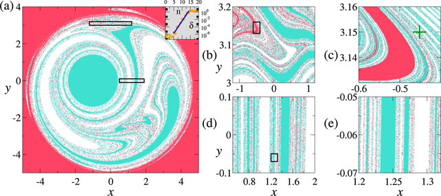
Figure 2. Exit basins for the unit disks centered at (−1, 0) (turquoise) and (1, 0) (white). Red corresponds to the initial positions of non-escaping particles. The parameters are ξ = 20, η0 = 2, and λ = 0.8. (a) Domain [−5, 5] × [−5, 4]. (b) Magnification of the domain inside the upper rectangle shown in (a). (c) Magnification of the domain inside the rectangle in (b). (d) Magnification of the domain inside the lower rectangle shown in (a). (e) Magnification of the domain inside the rectangle in (d). Inset of panel (a): distance δ between a pair of initially close particles (initial distance 2 × 10⁻⁷) as a function of the iterate n. The initial positions of these particles are shown (+ symbol) in panel (c) and each of them belongs to a different exit basin. The scaling provides an estimate for the corresponding local finite-time largest Lyapunov exponent, h ≃ 1.52.
Download figure:
Standard image High-resolution imageAs a measure of sensitive dependence on initial conditions, we show in the inset of figure 2(a) the time evolution of the distance δ(n) between a typical pair of initially close orbits. The scaling in the phase of exponential separation is described by a positive local finite-time largest Lyapunov exponent.
To quantify the geometrical complexity of the set of initial conditions of non-escaping orbits suggested by figure 2, it is instructive to apply the modified uncertainty algorithm to line segments chosen in panels figures 2(b) and (d). This is the content of figures 3(h) and (a), respectively. We see that an effective fractal dimension is observed for many orders of magnitude of the scale parameter . We also observe that, at small scales, the codimension decreases. Note that, in accordance with what we expect from plots figures 2(c) and (e), the decrease in the codimension takes place at different scales for the different line segments. In panel figure 3(h), the double precision we use is sufficient to illustrate the asymptotic behavior where the codimension is zero. In panel figure 3(a), in contrast, we only see the initial decrease of the codimension, and the asymptotic behavior is not apparent under the use of double precision.

Figure 3. (a) and (h) Estimation of the codimension of the set of non-escaping solutions using the modified uncertainty algorithm. The initial conditions are taken on the line segments y = 0, x ∈ [0.5, 2] (a) and y = 3.15, x ∈ [−1.2, 1.2] (h). (b)–(g) Negative of the inverse escape time τe as a function of x for y = 0 and y = 3.15, respectively, in panels (b)–(d) and (e)–(g). The parameters are the same as in figure 2.
Download figure:
Standard image High-resolution imageAnother measure of the complexity suggested by figure 2 is given by the analysis of the escape time τe, defined in subsection 2.3, as a function of the position. Panels (b)–(d) of figure 3 show the behavior of τe on the line segment considered in panel figure 3(a), while panels (e)–(g) refer to the behavior of τe on the line segment considered in panel (h). We choose to plot −1/τe rather than τe itself because our system contains many orbits for which τe = ∞. It is worth noting the qualitative similarity between plots (d) and (e), where one observes peaks at the level −1/τe = 0 indicating the presence of never-escaping solutions. The fact that these panels correspond to different scales illustrates the dependence of the behavior of τe on the phase space position. The plateaus at height 0 observed in panels (f) and (g) are indicative of the asymptotic zero codimension proven to hold true in panel (h) for small enough scales.
We now characterize the time-dependent escape rates. Figure 4 shows these rates for 10 choices of parameters. For each panel, we have chosen a fixed value for the pair (ξ, η0) and five different values of the decaying factor λ. Our first observation here is that, for fast decay (λ = 0.5, 0.6, and 0.7), the escape rates decay exponentially in time with exponent ln λ. This is also the case, for large n, when the decay velocity is moderate (λ = 0.8). To understand why the exponent ln λ holds, it is instructive to look at the parameter dependence of the non-decaying blinking vortex-sink system. As shown by Károlyi and Tél [16], for fixed values of ξ the chaotic saddle observed for moderate and large values of η is replaced by a regular (fixed-point) saddle when this parameter assumes smaller values. In other words, chaos requires a more vigorous regime (as far as the kinetic energy of the system is concerned) to occur. Now, as shown in the inset of the right panel of figure 4, for fixed ξ the escape rate is proportional to η in the range of this parameter for which the saddle is regular. Returning to the decaying system which is the object of the present work, for large n one necessarily has small ηn , implying that the saddle of the corresponding (snapshot) non-decaying system is regular. Since ηn = η0 exp(n ln λ), the fact that the exponent ln λ describes the asymptotic decay of κ(n) is just a consequence of the observation that the decaying system transiently emulates each of the corresponding (η = ηn ) non-decaying systems. For fast and moderate decay, the system approaches the asymptotic regime after a few iterates of the map, allowing that regime to be numerically observable.

Figure 4. Time dependence of the instantaneous escape rate κ(n) as evaluated from a set of particles randomly chosen with uniform distribution on the straight line segment  . The legends on the left panel are also valid for the right one. Inset: escape rate for the non-decaying blinking-vortex system in the range of parameters where the saddle is regular and consists of a single hyperbolic point.
Download figure:
Standard image High-resolution imageFor slow decay of energy (large λ), the asymptotic regime is not observed numerically and the time evolution of the escape rate displays a rather complex behavior. This is seen in both panels of figure 4 for λ = 0.9. The reason is that the system spends a long time in the range of ηn for which the corresponding non-decaying systems display a chaotic saddle. In that range, the non-decaying system exhibits a nontrivial parameter dependence. In particular, for fixed ξ the escape rate can be a nonmonotonic function of η [16]. The results shown in figure 5 illustrate the case for another value of λ. They are consistent with our remark stated in the previous paragraph that the decaying system emulates the associated non-decaying systems. Indeed, the similarity between the graphs depicted in figure 5 suggests some degree of correlation between the escape rates of the decaying and corresponding (possibly with a delay) non-decaying systems.

Figure 5. Green: time dependence of the instantaneous escape rate κ(n) as evaluated from a set of particles randomly chosen with uniform distribution on the straight line segment (x, y) ∈ {−1} × (1, 2.8). The parameters are ξ = 10, η0 = 1, and λ = 0.933 033 ≃ (1/2)1/10. Orange: escape rate for the non-decaying blinking-vortex systems corresponding to parameters ξ = 10 and η(n) = λn
, as estimated by regression from a set of particles randomly chosen with uniform distribution on the straight line segment  . The continuous line segments joining subsequent points are drawn to facilitate the visualization.
Download figure:
Standard image High-resolution image
As already mentioned, the behavior of τe depends on the phase space position. As a consequence, so does the instantaneous escape rate κ(n). We have contemplated this fact in the captions of figures 4 and 5, where the line segments used for the evaluation of κ(n) were specified. The two conclusions supported by these figures, however, hold true in general and only require that the initial conditions are taken in the nontrivial part of phase space (i.e., where the basins of attraction of the two exits dominate). In fact, the arguments behind both the exponential decay of the escape rates (for small λ) and the nontrivial behavior of these rates (for λ close to 1) rely only on the observation that the decaying system mimics, at each time instant, its non-decaying analogue.
4. Discussion
We have studied the dynamics of fluid tracers in a model decaying incompressible flow with exit regions. We found that the two hallmarks of doubly transient chaos are present, namely, a positive finite-time (largest) Lyapunov exponent and an effective final-state sensitivity over many orders of magnitude of the length scale. Unlike undriven dissipative mechanical systems where doubly transient chaos was first described, however, decaying open flows exhibit escape rates that, at least in the asymptotic regime of large times, decrease (rather than grow) exponentially in time. Also, the set of non-escaping orbits of decaying flows (which is the analogue of basin boundaries of mechanical systems) has asymptotic (as → 0) codimension zero rather than one. We point that Misaki and Nagaosa also reported the observation of vanishing codimension at small scales in the different context of dissipative scattering of a charged particle in a specific potential [19].
We claim the generality of the results reported herein for decaying incompressible open flows. Indeed, our argument in section 3 implying that the set of initial conditions of non-escaping orbits is mostly composed of interior points can be easily adapted for this class of systems. The asymptotic vanishing codimension of this set follows immediately. As a word of caution, one should note that dye boundaries in incompressible open flows without sinks have a fractal and a nonfractal part [15]. This could reflect in the character of the finite-scale fractal dimension for the general case of decaying incompressible open flows. In fact, fractal and nonfractal components of the set of initial conditions of non-escaping orbits may in principle coexist in these systems.
On the other hand, the tendency of the decaying system to transiently mimic the corresponding snapshot non-decaying systems explains the behavior of the escape rates. In the case of slow decay, one can generally expect a nontrivial time dependence of this quantity, as the system spends a long time in the range of parameters for which the corresponding non-decaying system exhibits a chaotic saddle. In that range, there is no reason to expect for instance a monotonic dependence of the escape rate of the non-decaying system on the parameters, since this rate depends not only on the saddle's Lyapunov exponent but also on its information dimension (in accordance with the Kantz–Grassberger relationship [20]) and since complex bifurcation phenomena can take place, such as the appearance and destruction of KAM islands. Now, for fast and moderate decay of general incompressible open flows, it is reasonable to hypothesize that the system quickly reaches the parameter range where the saddle consists of a single fixed-point (in the discrete-time description of the dynamics). In this case, the escape rate is simply equal to the Lyapunov exponent of the fixed-point and its exponential decay is then an expected consequence of the exponential energy decay. For instance, in the blinking vortex-sink system, the kinetic energy scales with K2 + Q2 and, therefore, decays with e2nlnλ , while the escape rate is proportional to η and decays with enlnλ .
We have not addressed the fractal geometry of evolving sets of tracers such as those shown in figure 1. This is a question of practical importance when the tracers are active from the biological or chemical point-of-view. In fact, the productivity of such active tracers was shown to depend on the capacity dimension of those sets [5]. This finding provides an explanation for the so-called plankton paradox in oceanography [6]. The investigation of activity in decaying open flows is left for future work.
Another perspective of the work presented here is the study of the compressible dynamics of finite-size particles in decaying open flows. Both light [21] and heavy (aerosol) [9, 22] particles have been shown to either escape or approach attractors in non-decaying open flows. Neutrally buoyant finite-size particles, on the other hand, disperse around the unstable manifold of the chaotic saddle [23]. The study of aerosols in decaying open flows, in particular, is important for the understanding of the mechanisms underlying the airborne transmission of respiratory diseases such as Covid-19 [24].
Acknowledgments
The author is grateful to J-R Angilella, A E Motter and T Tél for illuminating conversations.
Data availability statement
The data that support the findings of this study are available upon reasonable request from the author.