the Creative Commons Attribution 4.0 License.
the Creative Commons Attribution 4.0 License.
 | 10 Aug 2021
EOT20: a global ocean tide model from multi-mission satellite altimetry
Michael G. Hart-Davis
Gaia Piccioni
Denise Dettmering
Christian Schwatke
Marcello Passaro
Florian Seitz
EOT20 is the latest in a series of empirical ocean tide (EOT) models derived using residual tidal analysis of multi-mission satellite altimetry at DGFI-TUM. The amplitudes and phases of 17 tidal constituents are provided on a global 0.125∘ grid based on empirical analysis of seven satellite altimetry missions and four extended missions. The EOT20 model shows significant improvements compared to the previous iteration of the global model (EOT11a) throughout the ocean, particularly in the coastal and shelf regions, due to the inclusion of more recent satellite altimetry data as well as more missions, the use of the updated FES2014 tidal model as a reference to estimated residual signals, the inclusion of the ALES retracker and improved coastal representation. In the validation of EOT20 using tide gauges and ocean bottom pressure data, these improvements in the model compared to EOT11a are highlighted with the root sum square (RSS) of the eight major tidal constituents improving by ∼ 1.4 cm for the entire global ocean with the major improvement in RSS (∼ 2.2 cm) occurring in the coastal region. Concerning the other global ocean tidal models, EOT20 shows an improvement of ∼ 0.2 cm in RSS compared to the closest model (FES2014) in the global ocean. Variance reduction analysis was conducted comparing the results of EOT20 with FES2014 and EOT11a using the Jason-2, Jason-3 and SARAL satellite altimetry missions. From this analysis, EOT20 showed a variance reduction for all three satellite altimetry missions with the biggest improvement in variance occurring in the coastal region. These significant improvements, particularly in the coastal region, provide encouragement for the use of the EOT20 model as a tidal correction for satellite altimetry in sea-level research. All ocean and load tide data from the model can be freely accessed at https://doi.org/10.17882/79489 (Hart-Davis et al., 2021). The tide gauges from the TICON dataset used in the validation of the tide model, are available at https://doi.org/10.1594/PANGAEA.896587 (Piccioni et al., 2018a).
- Article
(12741 KB) - Full-text XML
- BibTeX
- EndNote


The regular fluctuations of the sea surface caused by ocean tides have intrigued and fascinated scientists for centuries based on their influence on oceanic processes. Understanding ocean tides is vital for a variety of geophysical fields, with it being of particular importance in studies of the coastal environment and ocean mixing. Precise knowledge of ocean tides is also important for satellite altimetry and in determining high-resolution temporal gravity fields from, for example, the GRACE missions (Tapley et al., 2004).
In certain studies of non-tidal signals using satellite altimetry data, such as in sea-level and ocean circulation research, ocean tides need to be removed from the data signal to properly study these processes. These so-called tidal corrections are usually provided by ocean tide models that have been specially developed to predict the tidal signals throughout the global ocean. The ever-evolving and improving field of ocean tide modelling has resulted in significant leaps in the accuracy of estimations of ocean tides (Shum et al., 1997; Stammer et al., 2014). There are several ocean tide models that have been developed using different techniques and for different applications, with a comprehensive summary of these models being presented in Stammer et al. (2014). In general, ocean tides are known in the open ocean region to an accuracy of approximately 2 cm (Savcenko and Bosch, 2012); however, models show large discrepancies between one another and compared to in situ observations in the coastal region (Ray et al., 2011). Improvements continue to be made, with estimations significantly improving in the coastal and polar regions (Ray et al., 2019). Poorer results are seen in the coastal region due to poorly resolved bathymetry, the complexity of ocean tides and due to land contamination of satellite altimetry radar signals (Fok, 2012).
One type of ocean tide model, known as semi-empirical models, is derived from empirical harmonic analysis of satellite altimetry data relative to a reference model. These semi-empirical tide models rely heavily upon satellite altimetry data. Recently, significant advancements have been made to coastal altimetry in several fields including key improvements in correction fields, more detailed and coastal-specific data editing, and new schemes for radar echo analysis (retracking) (Cipollini et al., 2017). Piccioni et al. (2018b) demonstrated an improvement greater than 2 cm for single tidal constituents when using the ALES (Adaptive Leading Edge Subwaveform: Passaro et al., 2014) retracker that enhances the performances of sea level retrieval in the coastal region and the corresponding sea state bias correction (Passaro et al., 2018). The continued developments of altimetry in the coastal region coupled with the increased number of altimetry missions have had a positive impact on the ability of models to more accurately estimate ocean tides.
EOT11a (Savcenko and Bosch, 2012), the latest in a series of global ocean tide models developed at DGFI-TUM, is an example of a semi-empirical tide model developed using residual tidal analysis of multi-mission satellite altimetry. EOT11a exploits altimetry observations of the sea level anomaly (SLA) corrected using a reference ocean tide model (FES2004) to estimate the tidal harmonic constants. EOT11a showed significant improvements compared to the previous iterations of the model, EOT08a and EOT10a, with noticeable improvements being seen in the shallow water regions (Savcenko and Bosch, 2012). The model has continued to be developed, with regional studies being conducted by Piccioni et al. (2021) based on improvements being made in the coastal region. These improvements are largely driven by the progresses in accuracy and precision of altimetry measurements in the coastal zone and the use of the updated FES2014 (Lyard et al., 2020) tide model as the reference model for the residual tidal analysis.
In this paper, the latest global version of the EOT model, EOT20, is presented based on recent developments made in the field of tide modelling, coastal altimetry and the availability of an increased number of altimetry missions. The objective of the EOT20 model is to improve the accuracy of tidal estimations in the coastal region while remaining consistent in the open ocean. In Sect. 2, a description of the altimetry data used and how EOT20 is produced through residual tidal analysis is given. Following this, a comparison of the results of the EOT20 model with in situ observations and other global tide models is presented in Sect. 3, with a conclusion and summary given in Sect. 5.
The development of EOT20 focused on improving tidal estimations in the coastal region which has been a historically difficult region to accurately estimate tides. EOT20 follows a similar scheme as the former model, EOT11a, consisting of three major steps: the creation of an SLA product including the correction of a reference ocean tide model; the estimation of the residual tides based on this SLA product; and the combination of the reference model with the residual tides to form a new global ocean tide model. These three steps provide a summary of the creation of EOT20 which is expanded in the following sections.
Table 1The satellite altimeter data used in this study obtained from OpenADB at DGFI-TUM (Schwatke et al., 2014). The corrections listed in Table 2 are applied to all these missions. Most missions are retracked using the ALES retracker (Passaro et al., 2018), marked by ∗, with TOPEX and ERS using ocean ranges as provided in SGDR datasets.
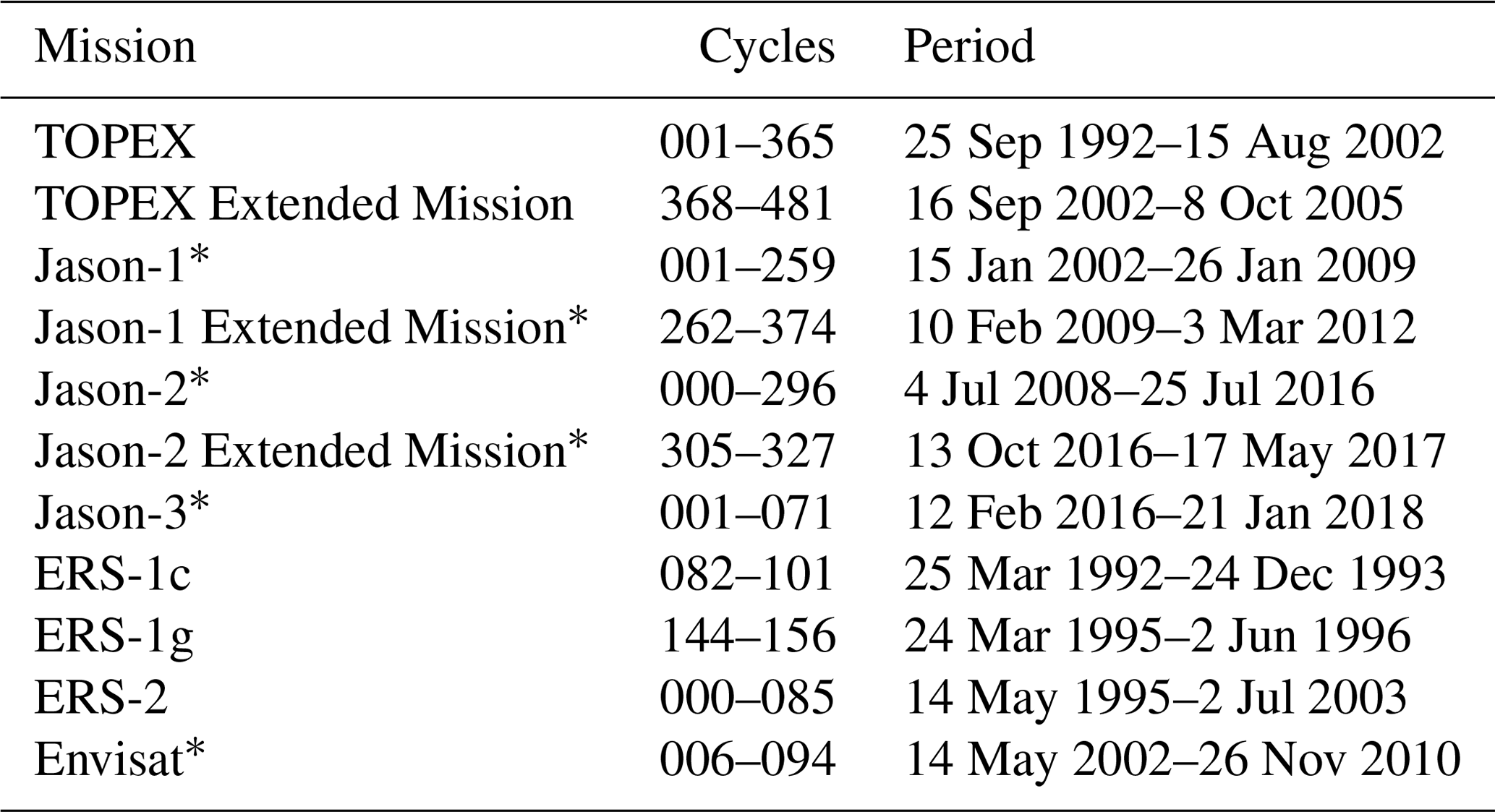
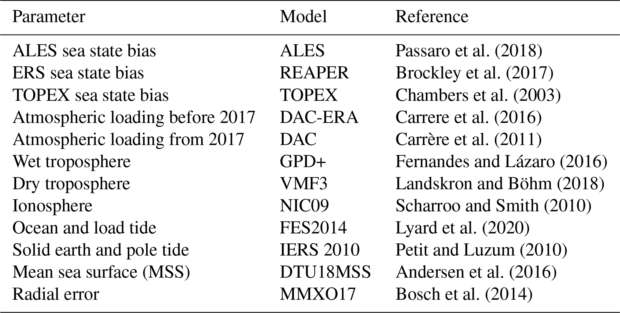
Table 2List of corrections and parameters used to compute SLA for tidal residuals estimation.
2.1 The altimetry SLA product
The tidal analysis is based on the analysis of SLA derived from satellite altimetry missions (Table 1) obtained from the Open Altimeter Database (OpenADB, https://openadb.dgfi.tum.de, last access: 5 August 2021, Schwatke et al., 2014). These missions are selected as they provide extended time series along similar altimetry tracks, with the Jason missions being a follow-on from TOPEX/Poseidon and Envisat a follow-on of the ERS missions, thus providing appropriate data for the estimation of tidal signals. The SLA from these altimetry missions is calculated according to that described in Andersen and Scharroo (2011):
where H is the orbital height of the satellite, R the range, MSS the mean sea surface and hgeo is the sum of the geophysical corrections (as listed in Table 2). For all of the missions, satellite orbits in ITRF2008 are used. For the ERS and TOPEX these are taken from GFZ VER11 (Rudenko et al., 2018), while for the Jason missions and Envisat CNES GDR-E solutions are used. The corrections used are chosen to optimise the estimations of the SLA in the coastal region, without harming the estimations in the open ocean regions.
The same corrections are used for each satellite altimetry mission to allow for consistency, with the only differences occurring in the sea state bias correction. The ALES retracker (Passaro et al., 2014) is applied to the Jason missions and the Envisat mission based on data availability at the time of running the model, with the other altimetry missions using the REAPER (Brockley et al., 2017) and TOPEX sea state bias corrections (Chambers et al., 2003). This discrepancy in the chosen retracker is designed to benefit from the ability of the ALES retracker in obtaining data closer to the coast which Piccioni et al. (2021) showed had positive improvements on the accuracy of the EOT tide model for the major tidal constituents compared to using the other retracked data. Therefore, depending on the retracker that is used, a coastal flag is implemented into the model that limits the distance to the coast. For missions using the REAPER and TOPEX retrackers, a coastal flag is implemented that restricts the use of SLA data up to 7 km from the coastline. For missions using the ALES retracker, however, this distance to the coast is decreased to 3 km (Passaro et al., 2021). An additional flag is also added limiting the absolute value of sea level anomalies to ± 2.5 m (Savcenko and Bosch, 2012). The altimetry data are further adjusted to account for radial errors estimated in the cross-calibration of the SLA data using the multi-mission crossover analysis approach presented in Bosch et al. (2014).
As shown in Table 2, the ocean and load tide correction for all missions is the FES2014 oceanic tide model. This is one of the major changes from the previous version of the global EOT model, EOT11a, which used one of the previous versions of the FES model, FES2004. The results of Lyard et al. (2020) showed considerable improvements in FES2014, particularly in the coastal and shelf regions. These improvements are largely driven by the improved efficiency of data assimilation and the accuracy of hydrodynamic solutions. It is, therefore, anticipated that large parts of the improvements made between the versions of EOT will be due to the improvement in the reference model.
Once all these corrections are applied, the SLA can be estimated for all 11 altimetry datasets which are then gridded onto a triangular grid based on the techniques presented in Piccioni et al. (2021). The triangular grids are chosen based on the efficiency of the model and allow for consistency of grid sizes throughout the ocean, thus not over-utilising data in regions of dense data availability. For each grid point, SLA values are collected within a variable capsize, with the radius, ψ (in km), of the capsize being a function of latitude (φ in degrees) where ψ = 165 − 1.5 (φ). Other capsize techniques are available based on a fixed or depth-based capsize, but they do not make significant changes to the results of the estimated tidal residuals and depreciate the efficiency of the model. The choice of the variable capsize is also to compensate for the greater data density available in higher latitudes.
Once collected, the data are then weighted using a Gaussian function based on the distance to the grid point. The use of data from multiple satellite tracks for each node provides a long SLA time series, which is important in reducing the aliasing effect and in decorrelating tidal signals with alias periods close to each other (Savcenko and Bosch, 2012). These issues occur due to the low temporal resolution obtained from satellite altimetry (e.g. the Jason missions only sample the same position once every 9915 d) resulting in tides not being properly estimated. The alias periods for the major tidal constituents for the Jason and the ERS orbits are presented in Le Provost (2001). The use of nodes with data from multiple altimetry missions, therefore, creates a long enough time series to improve the temporal resolution and reduce possible aliasing effects in the tidal estimations.
2.2 Residual tidal analysis
From the weighted SLA, residual tidal analysis is performed using weighted least-squares and the variance component estimation (VCE) for each grid point of the model. The least-squares approach is applied to the harmonic formula to derive the amplitudes and phases of single tidal constituents from the SLA observations. In EOT20, the 17 tidal constituents considered and computed are 2N2, J1, K1, K2, M2, M4, MF, MM, N2, O1, P1, Q1, S1, S2, SA, SSA and T2. The weighted least square analysis follows a standard procedure solving the following equation for each grid point (Piccioni et al., 2021):
with l being the vector of SLA values, A the design matrix, W the diagonal matrix of weights, and x the vector of unknowns. The unknowns of vector x are the in-phase and quadrature coefficients of the tidal constituents being considered, the sea level trend, and the constant values defined as the mean sea level from each specific mission at each node (Piccioni et al., 2021).
The VCE is implemented to allow for the combination of datasets from multiple satellite missions and allows for the appropriate weighting of different missions m, m = , (Savcenko and Bosch, 2012) based on their variances, to provide a more accurate estimation. The VCE method has been utilised in a variety of applications, and it was introduced into the previous global model, EOT11a (Savcenko and Bosch, 2012), which followed the formulation detailed in Teunissen and Amiri-Simkooei (2008) and Eicker (2008). The VCE is calculated using iterations as the unknowns, and the variances, σ, are initially unknown. The formulation is as follows:
with Nx and Ny equal to the weighted sum:
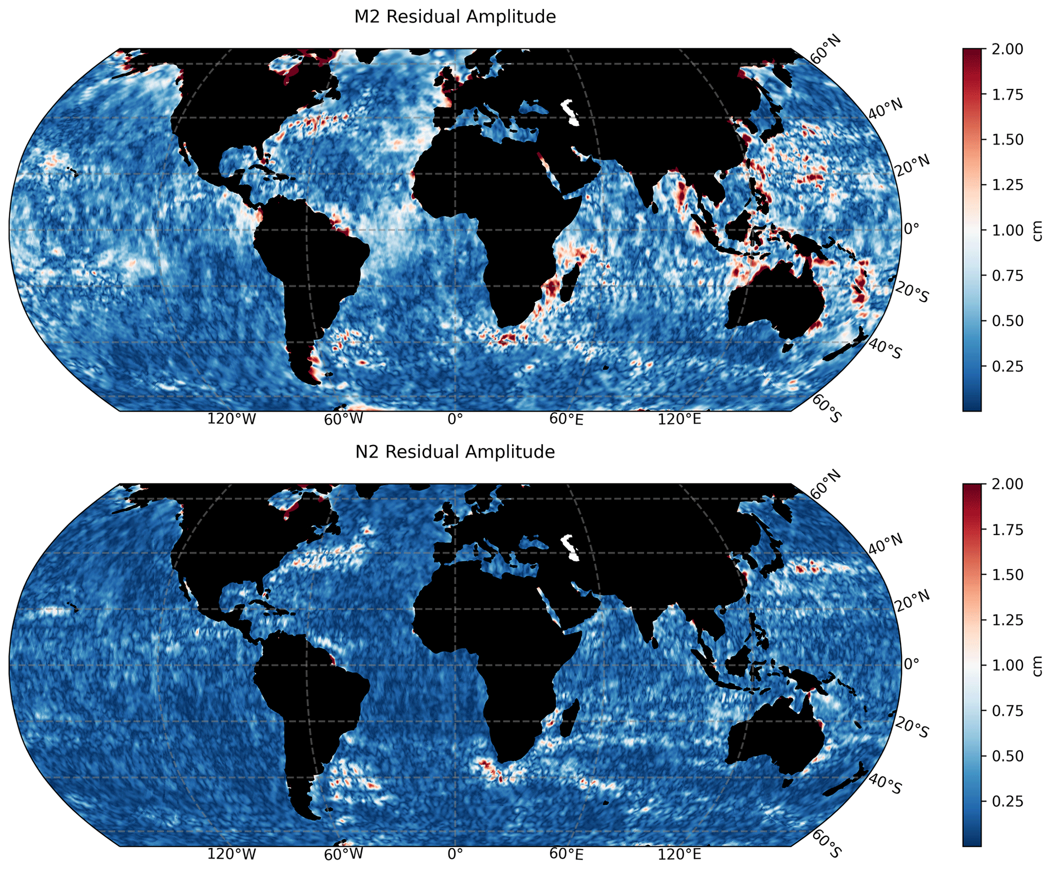
Figure 1Maps of the residual amplitudes of the M2 and N2 tidal constituents as estimated by residual tidal analysis.
The variances are iteratively calculated by
where rm is the partial redundancy with , being the vector of residuals, and Pbb is the dispersions matrix of measurements (Savcenko and Bosch, 2012). Following the residual analysis, significant residual signals were obtained for all of the tidal constituents. For the M2 and N2 tides (Fig. 1), for example, the residual amplitudes can exceed 2 cm with the largest residual tides being seen in the coastal region. Relatively high residual tides are also seen in the western boundary currents, such as the Agulhas Current and the Gulf Stream.
The tides observed are the residual elastic tides that consist of both the ocean and the load tides. Therefore, additional analysis has been done to separate these two components for further analysis. There are several techniques that are described that make this possible (e.g. Francis and Mazzega, 1990) with EOT using the method presented in Cartwright and Ray (1991). This method involves using the complex elastic ocean tide admittance decomposed in complex spherical harmonics as described by Savcenko and Bosch (2012):
The ocean spherical harmonic admittances of the load tides are described as
where with . The love numbers, , were taken from Farrell (1972) with ρw and ρe being the density of the ocean and earth. After synthesis of the load tides, the residual ocean tides were computed as the difference between the load and the elastic tide, .
2.3 Model formation
Once the ocean and load tide residuals are produced, the full tidal signal is restored by adding the residuals to the FES2014 tidal atlas. The residuals are interpreted onto a 0.125∘ resolution grid with the FES2014 model interpreted onto the same grid resolution. The outputting of the data onto a regular grid is simply done to allow for an easy combination with the FES2014 model as well as to be more user friendly. The north–south extent of the model extends 66∘ N and 66∘ S, with the model defaulting to the FES2014 tides in the higher latitudes. This extent is chosen due to the limited altimetry data further beyond this latitudinal band and the difficulty in modelling the tides in the polar regions. Dedicated studies to the Arctic region such as that of Cancet et al. (2019) demonstrate the complexity of modelling ocean tides in the polar regions and emphasise their importance for satellite altimetry.
Future iterations of the EOT model will tackle the estimation of tides in the higher latitudes. A land–sea mask was added to the model based on the GMT that uses the GSHHG coastline database (Wessel and Smith, 1996), which is a high-resolution database that contains information about coastlines as well as lake and river boundaries. These data have a mean point separation of 178 m which has been interpolated to a 0.125∘ resolution for use in the EOT20 model. In complex coastal regions, such as regions with islands or in semi-enclosed bays, properly defining the coastlines becomes extremely valuable when validating the model against in situ tide gauges. This is largely a result of artifacts forming when estimating tides in regions where the coastline has not been properly defined. For example, the Cook Strait between the two islands of New Zealand provides a unique coastal structure which shows a sharp change in the amplitude of major tides (e.g. M2, N2, S2 and K2 as shown in Walters et al., 2001) and, therefore, requires a more accurate coastline definition. Preliminary studies of EOT20 (not shown) demonstrated that for tide gauges within the Cook Strait the root sum square (RSS) difference between the model and tide gauges was reduced by 0.2 cm for the eight major tidal constituents when applying a more accurate land–sea mask. An overall reduction in RSS is seen throughout the ocean when using an accurate land–sea mask.
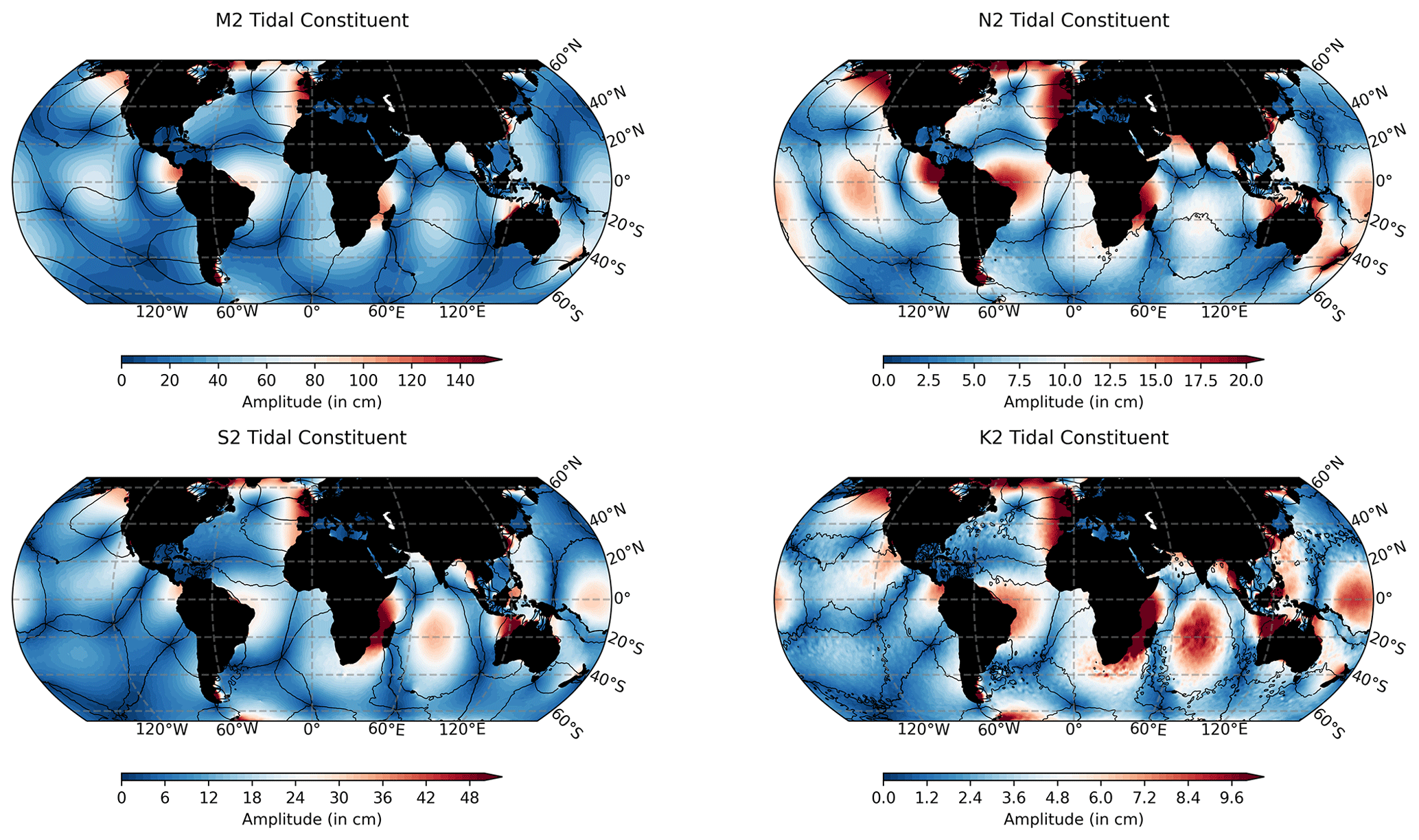
Figure 2The amplitude (in cm) and the phase (in 60∘ increments) of four ocean tidal constituents produced by the EOT20 model.
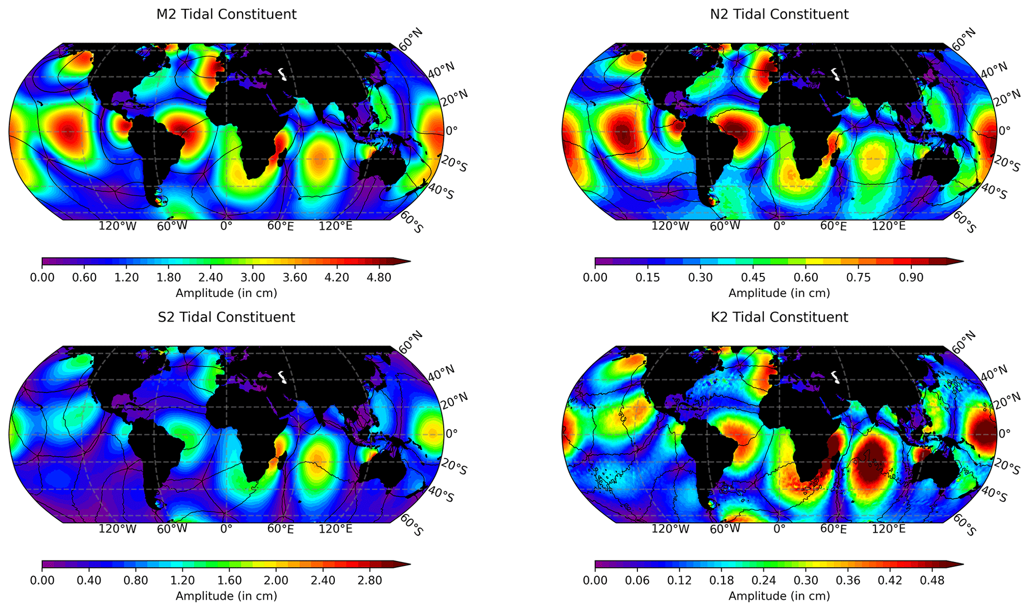
Figure 3The amplitude (in cm) and phase (in 60∘ increments) of the four load tide constituents produced by the EOT20 model. It should be noted that EOT20 does not make an estimation for the load tides on land.
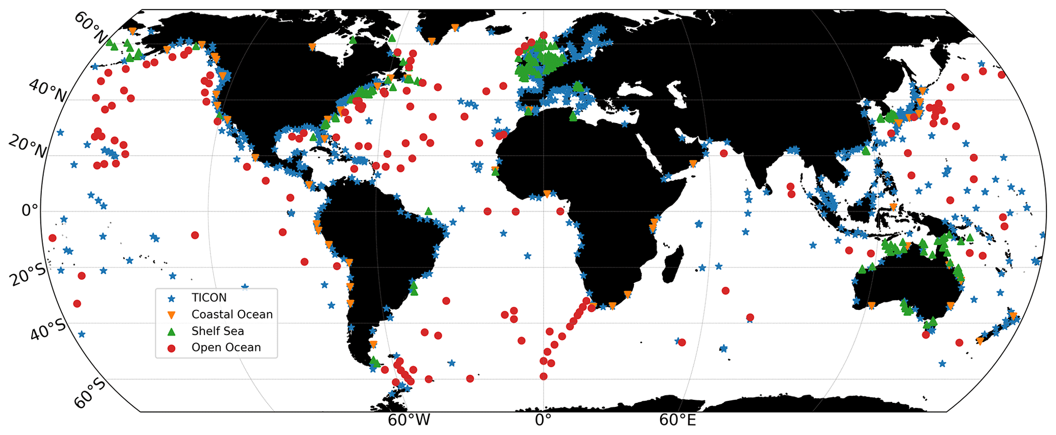
Figure 4The global array of tide gauges and ocean bottom pressure sensors that were used in the validation of the EOT20 model from the TICON dataset and from Stammer et al. (2014): the coastal ocean, shelf sea and open ocean datasets.
3.1 The global EOT20 model
EOT20 presents global estimations of 17 tidal constituents with these tidal atlases being available from https://doi.org/10.17882/79489 (Hart-Davis et al., 2021). Global atlases of both ocean and load tides are provided, containing information about the amplitudes and phases as well as the real and imaginary components for all of the tidal constituents. Here, the ocean (Figs. 2 and A1) and load (Figs. 3 and A2) tides from EOT20 are presented. Building on from EOT11a an additional four tidal constituents have been estimated in the EOT20 product. which are the T2, J1, SA and SSA tidal constituents. The SSA and SA tides are included in the EOT20 model data, but users should be aware that these tides include the full signal at these periods, i.e. gravitational as well as meteorological tides. Thus, caution should be taken when interpreting the results of the tidal correction when these two tides are included as they will likely remove the seasonal signals seen in the altimeter data.
The EOT20 model follows the framework of the EOT11a model when estimating the tide via residual analysis. However, significant changes and additions have been done to EOT20 with the objective of improving coastal estimations. These changes are in the reference tide model used in the residual analysis, the use of more recent developments in coastal altimetry (e.g. the development of the ALES retracker Passaro et al., 2014), the increased coverage of satellite altimetry based on the launching of further missions (e.g. Jason-3), the use of an accurate land–sea mask onto the model output data, and using a triangular grid for the residual analysis. These additions all combine to optimise the estimation of ocean tides in the EOT20 model.
3.2 Tide gauge comparison
Since the 1800s, tide gauges have been used to study the ocean tides and the variation in sea level. Over the years, more and more tide gauges have been installed around the world, resulting in a vast array. This comprehensive record of tide gauges can be used to evaluate the changes in sea level over time as well as to better understand the ocean tides. Tide gauges, therefore, provide a suitable source of data in the validation of ocean tide models, particularly in the coastal region. There are limitations particularly in the distribution of tide gauges, with certain regions containing a vast number of tide gauges (e.g. in northern Europe) and some regions containing little to no data (e.g. the Mozambique Channel). Furthermore, tide gauges are mostly restricted to the coastal region and, therefore, do not provide sufficient observations of the open ocean region. With that in mind, Ray (2013) estimated tidal constants from bottom pressure stations in the open ocean regions which have been used to compare and assess the accuracy of global ocean tide models (Stammer et al., 2014). These data are combined with coastal and shelf data from Stammer et al. (2014), henceforth referred to as the R. Ray dataset, as well as the TICON dataset (Piccioni et al., 2019) to create a comprehensive dataset of tidal constants (shown in Fig. 4) to evaluate the accuracy of the EOT20 model throughout the global ocean. As the tide gauge and bottom pressure sensor distributions are already split into coastal, shelf and open ocean tide gauges from Stammer et al. (2014), the TICON dataset is also divided into three regions with the coast being defined as any tide gauges found shallower than 10 m, the shelf defined as being from 10 to 100 m depth and open ocean being anything deeper than 100 m. This is done to assess how the model performs in the coastal region, a historically difficult region to model accurately.
Table 3The rms, in cm, of the tide gauge analysis of 1226 tide gauges for the EOT20 model as well as several other global ocean tide models. The values marked in bold indicate the model with the smallest rms for each row.
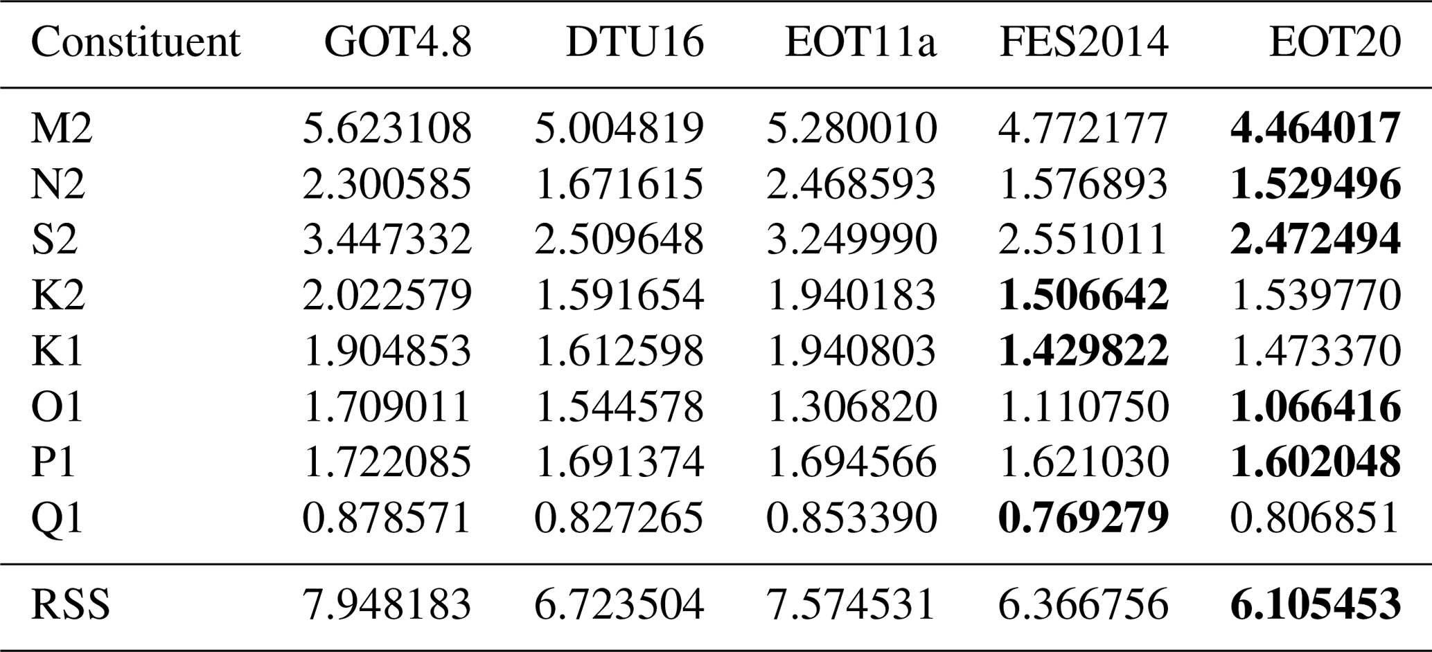
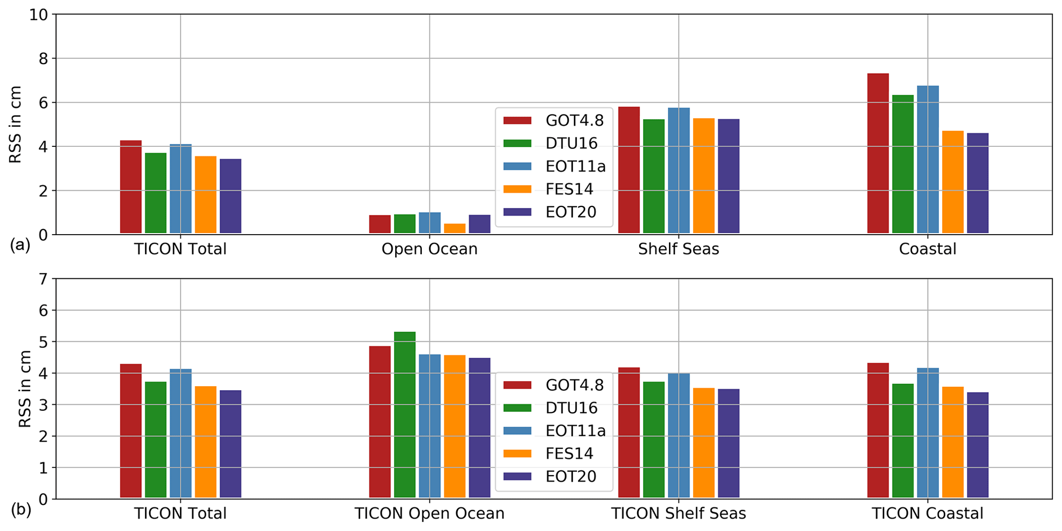
Figure 5(a) RSS (cm) between the tide gauge databases and the global tidal models, for the eight major tidal constituents. (b) The RSS of subset regions of the TICON database as well as the full database.
Several major ocean tide models are also compared to the same tide gauges in order to act as reference to the ability of the EOT20 model. The models used are EOT11a (Savcenko and Bosch, 2012), FES2014 (Lyard et al., 2020), GOT4.8 (Ray, 2013) and DTU16 (Cheng and Andersen, 2017). To provide suitable comparisons, duplicate tide gauges were removed and restrictions were implemented based on the model characteristics (i.e. only tide gauges between 66∘ S and 66∘ N were used). This results in 1226 tide gauges and bottom pressure sensors being available for validation of the models. The TICON dataset provides standard deviations for individual constituents, with the average standard deviation for the tide gauges used in this study being 0.09 mm. No uncertainty estimates are provided in the R. Ray dataset. It should also be noted that 230 of the tide gauges used in this study are assimilated into the FES2014 model. The root mean square (rms) and root sum square (RSS) are then estimated for the eight major tidal constituents (M2, N2, S2, K2, K1, O1, P1 and Q1) which are commonly available from the tide models studied, following the techniques presented in Stammer et al. (2014).
The comparison between EOT11a and EOT20 shows a significant improvement in the EOT20 model for the full dataset (Table 3). This is consistent for all of the tidal constituents, with a major improvement seen in the M2 tide (0.8 cm) and the S2 tide (0.8 cm). For all of the regions (Fig. 5), EOT20 continues to show improvements compared to EOT11a particularly in the coastal region with a mean RSS reduction of 2.2 cm. In the coastal region, EOT20 shows a reduced rms for all the tidal constants with large reductions occurring again for the M2 (1.3 cm) and S2 tide (1.1 cm) with significant reductions in the K2 (0.5 cm) and N2 (1.3 cm) tidal constituents. Reductions in RSS are also seen in the other regions; however, the magnitude is not as large as in the coastal region, which results in smaller differences seen in the overall dataset (Table 3). This suggests that the adjustments and additions made to the EOT model, such as the incorporation of the ALES retracker in the estimation of the SLA, produce substantial differences to the performance of the model in the coastal region without harming the performances in other regions.
EOT20 also shows a reduced RSS when compared to the other global models, particularly compared to the reference model, FES2014. The largest improvement comes in the M2 tidal constituent while the results for the remaining tidal constituents are quite consistent between FES2014 and EOT20. In the coastal region, EOT20 shows significant improvements compared to the other models, being approximately 0.2 cm better than the closest model in this region (Fig. 5). The better performance of EOT20 seen in Table 3, therefore, can mostly be put down to the results seen in the coastal region. This is further highlighted in the TICON dataset, which contains significantly more coastal tide gauges compared to the other two regions (Fig. 5). In this dataset, EOT20 shows a reduction in rms for the M2 tidal constituent of 0.3 cm compared to the next best model (FES2014). For the remaining tidal constituents, EOT20 and FES2014 never vary by more than 1 mm in terms of rms values. This improvement compared to FES2014 is mainly seen in the coastal region (Fig. 5), which is in line with previous regional studies of EOT done using FES2014 as the reference tide model and the ALES retracker (Piccioni et al., 2018b).
In the shelf region, the reduction of rms in the M2 tide from EOT20 is still seen compared to FES2014 but reduces to less than 1 mm. The RSS of EOT20 and FES2014 match one another, only differing by less than 0.005 mm, while DTU16 is within 1 mm of both of these models in this region. This suggests that these three tide models are on par with one another in the shelf regions. In the open ocean, the similar results continue with the RSS spread between all of the models not exceeding 2 mm, with the only exception being the strong performance of the FES2014 model in this region. FES2014 outperforms the next best tide model, EOT20, by showing a reduction in RSS of 4 mm. For all of the tidal constituents, FES2014 shows a lower rms compared to EOT20 in the open ocean region.
The constituents not included in the previous analysis are compared to the FES2014 model and the TICON tide gauge dataset (presented in Fig. A3). Only the TICON tide gauge dataset is used based on the availability of appropriate tidal constituents for the analysis. For six of the seven tidal constituents presented here, the two tide models show similar results to one another. For the J1 and M4 constituents, a slight improvement can be seen from EOT20 when compared to FES2014 while for the remaining tidal constituents, EOT20 shows a higher rms. Despite showing similar results for these constituents, it is clear that the solutions of EOT20 for these tides are still imperfect with the higher rms values caused by the difficultly to estimate the small signals of these tides from an altimetry perspective as well as due to the effects of temporal aliasing. Through the increased number of altimetry missions as well as improved processing techniques, these minor tidal constituents will be better estimated in future iterations of the EOT model. It should also be noted that the assessment of the models using in situ tide gauges themselves would benefit from additional high-quality extended time series in order to more accurately estimate the long-period constituents presented here (MM and MF).
The S1 tidal constituent is the relatively worst performing tidal constituent from the EOT20 model with an increased rms of 0.2 cm compared to FES2014. This problematic result is likely influenced by errors from the ionospheric correction, NIC09, that is used in the creation of the SLA product, which may leak into the estimation of the ocean tides (Ray, 2020). The ionospheric correction used in EOT20 is aimed at optimising the performance of the tide model in the coastal region; however, this may be negatively impacting the estimation of certain tidal constituents, like the S1 tide. Furthermore, Ray and Egbert (2004) discuss the impact that geophysical corrections (mainly inverse barometer and dry troposphere) have on the estimations of the S1 tide from altimetry data. A future study of the EOT model will investigate the use of different geophysical corrections to optimise the estimation of ocean tides with particular focus on the S1 tidal constituent.
The results of the tide gauge and ocean bottom pressure analysis suggest rather encouraging results from the EOT20 model. The estimated tidal constituents of EOT20 are notably improved compared to the previous EOT11a model. The performance of the model in the coastal region is noteworthy particularly in the representation of the M2 tidal constituent. Furthermore, the model remains on par with the other global tide models in the open ocean and shelf regions.
3.3 Sea level variance reduction analysis
In order to further assess the models ability, sea level variance reductions of three satellite altimetry missions were assessed and are presented. As seen in Fig. 4, tide gauges and ocean bottom pressure do not provide full coverage of the open ocean, so comparing the sea level variances of ocean tide models provides a suitable assessment of the performances of the models. The missions chosen are Jason-2 and Jason-3, which are used in the residual tide analysis as well as SARAL, which is not used in the analysis. A few steps are required in order to estimate sea level variance reduction. First, the along-track SLA is estimated using the corrections listed in Table 2 with the only differences being in the ocean and load tide correction. For this correction, two tide models (EOT11a and FES2014) were used to be compared to EOT20. The SLA for each cycle of all three missions was then estimated and then gridded onto a 4∘ grid. Once done, the variance of each of the SLA products was estimated (Savcenko and Bosch, 2012).
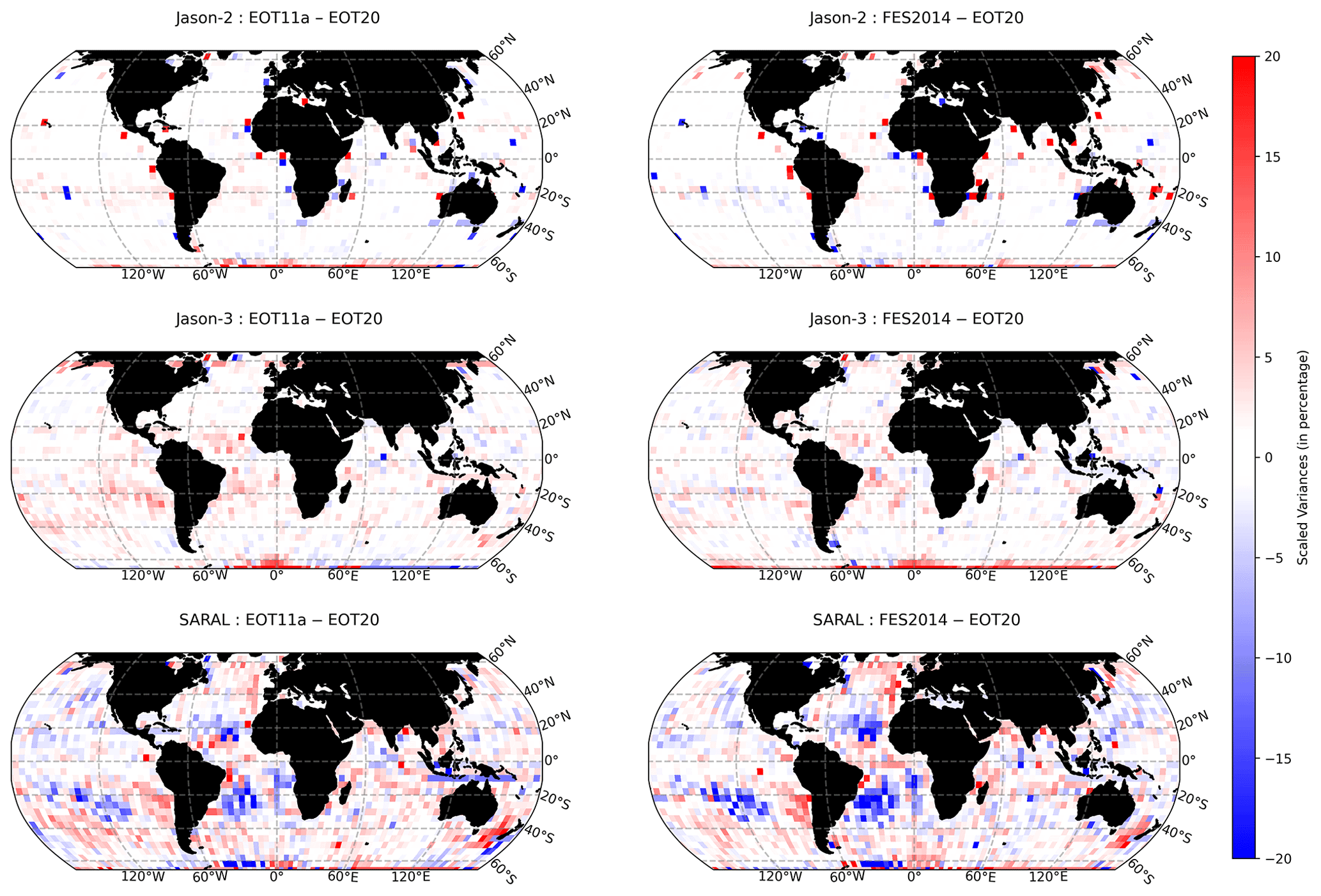
Figure 6The global scaled SLA variances differences for Jason-2, Jason-3 and SARAL in percentages. The colour bar is chosen for ease of understanding with the variance differences scaled to highlight the differences between the results. The colours are chosen so that when there are regions of red colours EOT20 shows a lower variance, while when regions are blue the other tide model (EOT11a or FES2014) has a lower variance.
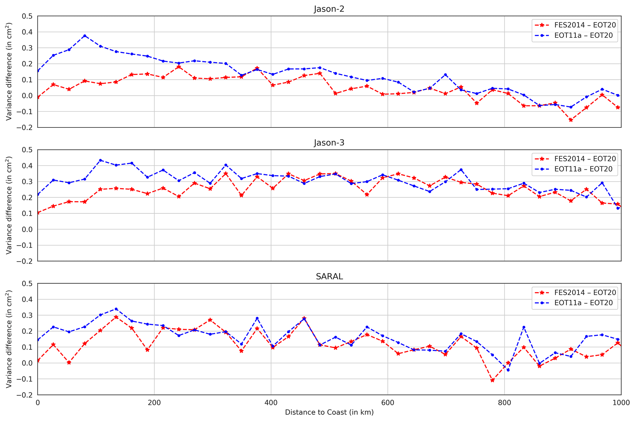
Figure 7A line graph showing the mean SLA variance differences between the tide models as a function of distance to coast (in km) for all three satellite altimetry missions. The red line represents FES2014 − EOT20, while the blue line represents EOT11a − EOT20.
Figure 6 presents the results of the scaled SLA variance differences between the three tide models. For the Jason-2 mission, which is the mission with the most cycles, the SLA variance differences between all tide models are very similar to one another with EOT20 showing an overall mean-variance reduction of 0.054 and 0.026 cm2 when compared to EOT11a and FES2014 respectively. The largest discrepancy is around 60 to 66∘ south, where EOT20 shows a lower SLA variance compared to EOT11a and FES2014. When looking at how the SLA variance differences change based on the distance to coast for Jason-2 (Fig. 7, top), it can be seen that EOT20 shows the largest reduction of variance in the coastal region. This is particularly the case when looking at the differences between EOT11a, with EOT20 reducing the variance by approximately 0.4 cm2 in the first 100 km from the coast. As they move further from the coast, the difference between the two models begins to reduce and converge towards zero. The variance difference between FES2014 and EOT20 shows similar results. Closer to the coast, EOT20 shows a reduced variance compared to that of FES2014 with differences exceeding 0.1 cm2, but as they move further from the coast the difference between the two models converges towards zero. Like with the EOT11a model, FES2014 begins to show a reduced variance compared to EOT20 800 km from the coast.
For the Jason-3 mission, a reduction in SLA variance can be seen from the EOT20 model, with the discrepancies between the models again being very small (Fig. 6). The mean-variance reduction of EOT20 is 0.092 and 0.089 cm2 when compared to EOT11a and FES2014 respectively. The variance reduction can be seen throughout the ocean, with larger reductions in the coastal region (Fig. 7, middle). Like in the Jason-2 mission, the variance differences decrease further away from the coast. Although the variance reduction diminishes further from the coast, unlike in the other two missions EOT20 shows continued variance reduction throughout the ocean.
The SARAL mission presents differing results from those seen in the Jason missions. It should be noted that SARAL has considerably fewer cycles and has a different orbit compared to the Jason missions. However, the results still provide valuable insights into the performances of the models. When looking at the scaled variance differences, the results become a bit more variable between the models with EOT20 showing reductions in variance in regions such as the Indian Ocean and the North Atlantic Ocean but showing increased variance in regions such as the South Atlantic Ocean and the South Pacific Ocean. Overall, EOT20 shows a mean reduction of variance compared to EOT11a of 0.129 cm2 despite EOT11a outperforming the model in certain regions. The mean-variance reduction of EOT20 compared to FES2014 is 0.035 cm2; however, there are regions where FES2014 shows better performance, particularly in the South Atlantic. Again, the overall reduction in variance is largely driven by the models' performance closer to the coast (Fig. 7, bottom) with reductions compared to EOT11a and FES2014 exceeding 0.3 and 0.2 cm2 respectively closer to the coast, while these differences reduce towards zero further away from the coast.
The ocean and load tides from EOT20 are available at https://doi.org/10.17882/79489 (Hart-Davis et al., 2021). The GMT data used to create the land–sea mask can be found at http://gmt.soest.hawaii.edu (last access: 5 August 2021). The satellite altimetry data used in the model creation can be found at https://openadb.dgfi.tum.de/ (last access: 5 August 2021). The tide gauges from the TICON dataset used in the validation of the tide model are available at https://doi.org/10.1594/PANGAEA.896587 (Piccioni et al., 2018a).
In this study, an updated version of a global ocean tide model, EOT20, is presented. Model developments were aimed at updating the previous model, EOT11a, with a focus on improving the coastal estimations of ocean tides by utilising recent developments in coastal altimetry, particularly the use of the ALES retracker and sea state bias correction. In the residual analysis, SLA data are gridded into a triangular grid aimed at increasing the efficiency of the model and thus better-describing tides in the coastal and higher latitudinal regions. A further update was in the use of a newer version of the reference model (FES2014) for the residual analysis performed to create the EOT20 model, which showed significant improvements to the previous reference model used, FES2004 (Lyard et al., 2020).
To evaluate the performance of the EOT20 model, validation against in situ observations and through sea level variance analysis was done. First, the models performance was compared with tide gauges and ocean bottom pressure sensors for the eight major tidal constituents. The results suggested that EOT20 showed significant improvements compared to EOT11a throughout the global ocean, with major improvements being seen in the coastal region. Furthermore, when compared to other global ocean tide models, EOT20 had the lowest overall RSS for the major eight tidal constituents, In particular, improvements are seen in the coastal region, where EOT20 shows a reduced RSS of 0.2 cm compared to the closest model (FES2014). The rms differences between individual constituents show that EOT20 and FES2014 show clear improvements for all the tides compared to the other global models. EOT20 and FES2014 each had the lowest rms for half of the major tidal constituents presented, with the largest reduction in rms being seen in the M2 tide from EOT20. This positive performance was largely driven by the improved accuracy of the model compared to observations in the coastal region. In the shelf and open ocean regions, EOT20 was on par with the best tide models in these regions, DTU16 and FES2014, but there is still room for improvement compared to the FES2014 model in the open ocean.
The additional tidal constituents provide valuable data for the creation of the tidal correction used for satellite altimetry. The results of these additions show positive results compared to the FES2014 model, but improvements can still be made in determining some of these tides, particularly the S1 tidal constituent. Further investigations will be done at DGFI-TUM into the estimation of additional minor tidal constituents as well as the optimisation of the current estimations.
The sea level variance analysis continued to show positive results for EOT20. EOT20 reduced the mean variance compared to both FES2014 and EOT11a for all three satellite altimetry missions studied. Again, the largest reason for the improvement was seen in the coastal region with EOT20 showing similar results compared to the other models in the open ocean regions. These results of the new EOT20 model suggest that it will serve as a useful tidal correction for satellite altimetry.
Errors resulting from tide models are considered to be one of the main limiting factors for temporal gravity field determination and the derivation of mass transport processes (Koop and Rummel, 2007; Pail et al., 2016). In the creation of EOT20, a first look into the uncertainties of residual tide estimations was done, but due to the unavailability of uncertainty estimations from the FES2014 model used as the reference model these uncertainties are incomplete and, therefore, are not presented. This is a topic of discussion and future development that will be assessed in future studies.
As the fields of coastal altimetry and ocean tides develop, the ideas and methods of improving the EOT model continue to grow. A clear next step for the EOT model is to assess its ability to estimate tides in higher latitudes by including more satellite missions (e.g. CryoSat-2) and to introduce further data such as synthetic aperture radar altimetry from Sentinel-3. Furthermore, more recent developments in the estimation of internal tide models (Carrere et al., 2021) suggest that improvements may be made to the estimation of ocean tides from residual analysis when the internal tidal correction is applied to the SLA data. These potential avenues of improvement will be addressed in future iterations of the EOT model.
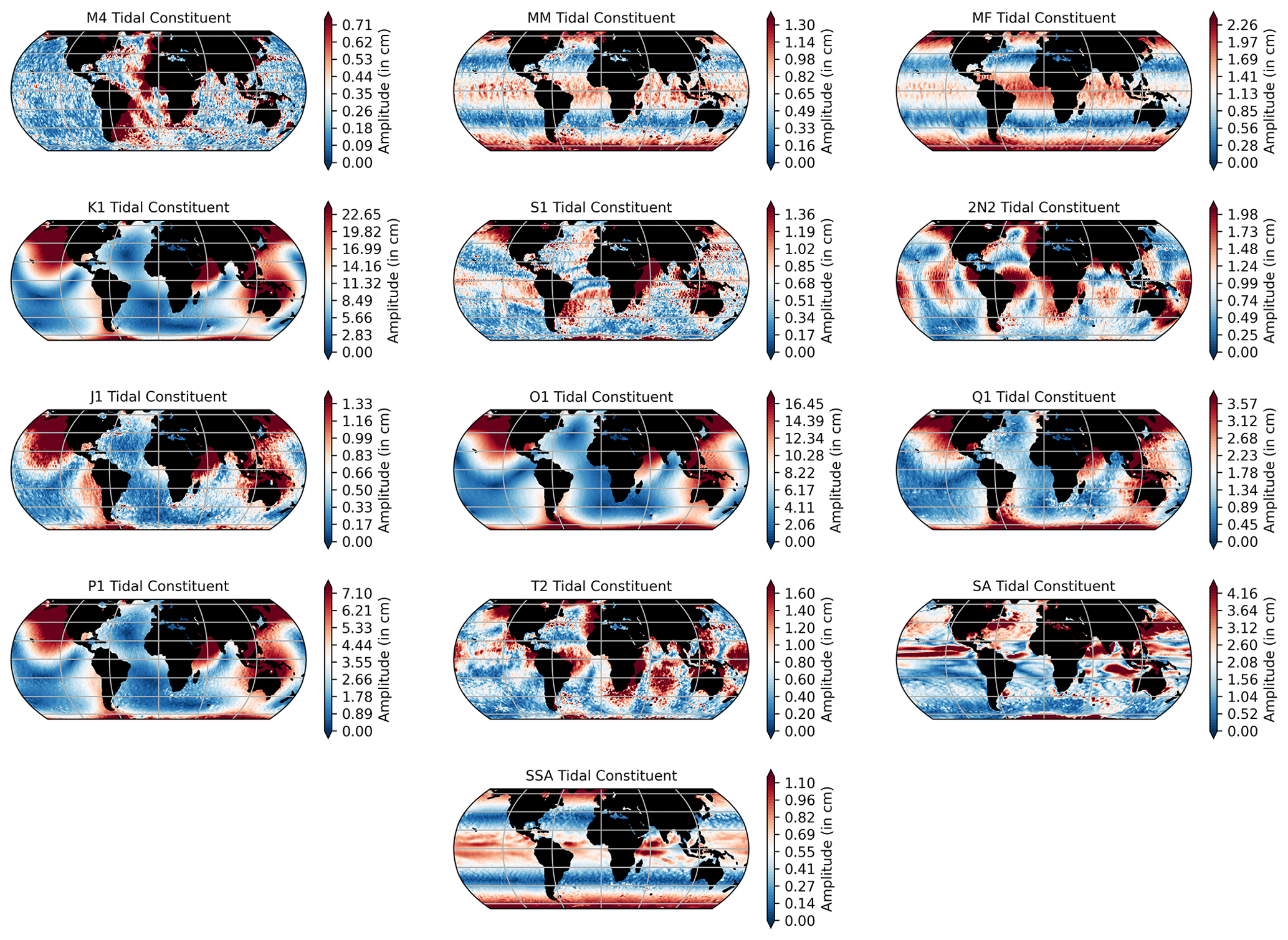
Figure A1The amplitude of the remaining ocean tide constituents provided by EOT20.
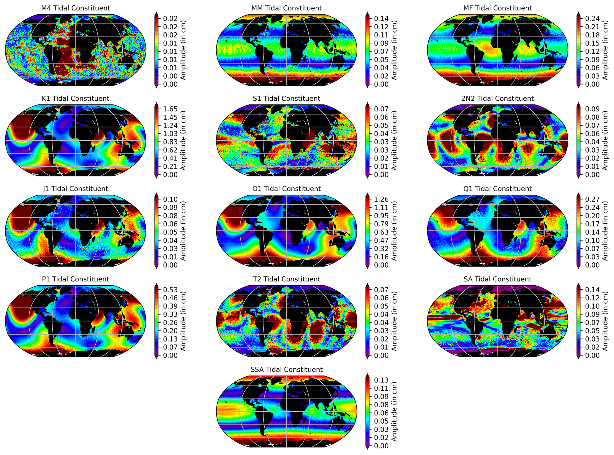
Figure A2The amplitude of the remaining load tide constituents provided by EOT20. It should be noted that EOT20 does not make an estimation for the load tides on land.
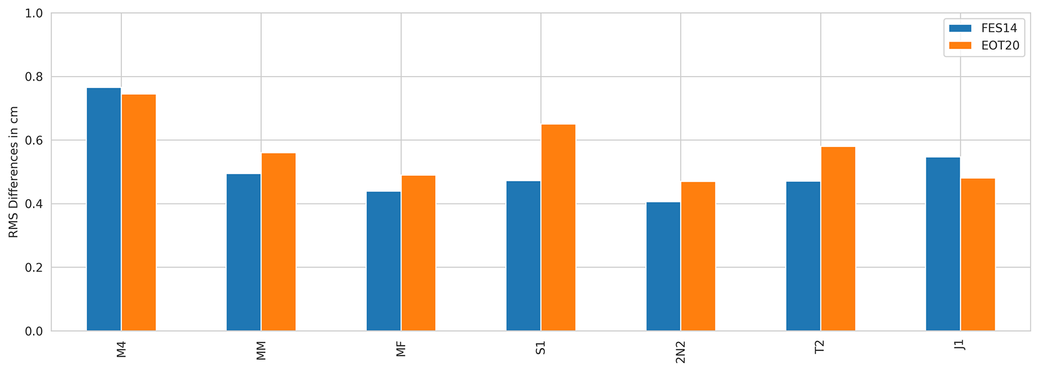
Figure A3The rms and RSS of the remaining tidal constituents compared to the tide gauge datasets for both FES2014 and EOT20. A total of 1059 of tide gauges were used for this analysis only from the TICON dataset due to the availability of appropriate tidal constituents.
MGHD wrote the manuscript and performed the validation of the model. MGHD and DD were involved with designing the study and in interpreting the results. MGHD and GP were responsible for the development of the EOT20 model. CS and DD were responsible for the appropriate satellite altimetry data and assisted in the variance reduction validation. MP is the author of the retracking algorithm and of the sea state bias correction used in the model. FS provided the resources making the study possible and coordinates the activities of the research group at DGFI-TUM. All authors read, commented and reviewed the final manuscript.
The authors declare that they have no conflict of interest.
Publisher's note: Copernicus Publications remains neutral with regard to jurisdictional claims in published maps and institutional affiliations.
The authors thank NOVELTIS, LEGOS, CLS Space Oceanography Division, CNES and AVISO for providing the FES2014 model. The authors would like to thank the anonymous reviewers for their input on the manuscript. We would also like to thank colleagues within the community for their comments on the model and results presented, particularly Sergiy Rudenko, Mathilde Cancet and Richard Ray.
This paper was edited by Giuseppe M. R. Manzella and reviewed by two anonymous referees.
Andersen, O. B. and Scharroo, R.: Range and geophysical corrections in coastal regions: and implications for mean sea surface determination, in: Coastal altimetry, edited by: Vignudelli, S., Kostianoy, A., Cipollini, P., and Benveniste, J., Springer, Berlin, Heidelberg, pp. 103–145, 2011. a
Andersen, O. B., Stenseng, L., Piccioni, G., and Knudsen, P.: The DTU15 MSS (mean sea surface) and DTU15LAT (lowest astronomical tide) reference surface, in: ESA Living Planet Symposium 2016, Prague, Czech Republic, 9–13 May, 2016. a
Bosch, W., Dettmering, D., and Schwatke, C.: Multi-mission cross-calibration of satellite altimeters: Constructing a long-term data record for global and regional sea level change studies, Remote Sens.-Basel, 6, 2255–2281, 2014. a, b
Brockley, D. J., Baker, S., Féménias, P., Martinez, B., Massmann, F.-H., Otten, M., Paul, F., Picard, B., Prandi, P., Roca, M., Rudenko, S., Scharroo, R., and Visser, P.: REAPER: Reprocessing 12 years of ERS-1 and ERS-2 altimeters and microwave radiometer data, IEEE T. Geosci. Remote, 55, 5506–5514, 2017. a, b
Cancet, M., Andersen, O., Abulaitijiang, A., Cotton, D., and Benveniste, J.: Improvement of the Arctic Ocean Bathymetry and Regional Tide Atlas: First Result on Evaluating Existing Arctic Ocean Bathymetric Models, in: Fiducial Reference Measurements for Altimetry, edited by: Mertikas, S. and Pail, R., Springer, Cham, Switzerland, pp. 55–63, 2019. a
Carrère, L., Faugère, Y., Bronner, E., and Benveniste, J.: Improving the dynamic atmospheric correction for mean sea level and operational applications of atimetry, in: Proceedings of the Ocean Surface Topography Science Team (OSTST) Meeting, San Diego, CA, USA, 16–21 October 2011, 19–21, 2011. a
Carrere, L., Faugère, Y., and Ablain, M.: Major improvement of altimetry sea level estimations using pressure-derived corrections based on ERA-Interim atmospheric reanalysis, Ocean Sci., 12, 825–842, https://doi.org/10.5194/os-12-825-2016, 2016. a
Carrere, L., Arbic, B. K., Dushaw, B., Egbert, G., Erofeeva, S., Lyard, F., Ray, R. D., Ubelmann, C., Zaron, E., Zhao, Z., Shriver, J. F., Buijsman, M. C., and Picot, N.: Accuracy assessment of global internal-tide models using satellite altimetry, Ocean Sci., 17, 147–180, https://doi.org/10.5194/os-17-147-2021, 2021. a
Cartwright, D. E. and Ray, R. D.: Energetics of global ocean tides from Geosat altimetry, J. Geophys. Res.-Oceans, 96, 16897–16912, 1991. a
Chambers, D., Hayes, S., Ries, J., and Urban, T.: New TOPEX sea state bias models and their effect on global mean sea level, J. Geophys. Res.-Oceans, 108, 3305, https://doi.org/10.1029/2003JC001839, 2003. a, b
Cheng, Y. and Andersen, O. B.: Towards further improving DTU global ocean tide model in shallow waters and Polar Seas, OSTST, in: Proceedings of the Ocean Surface Topography Science Team (OSTST) Meeting, Miami, FL, USA, 23–27 October 2017. a
Cipollini, P., Benveniste, J., Birol, F., Fernandes, M. J., Obligis, E., Passaro, M., Strub, P. T., Valladeau, G., Vignudelli, S., and Wilkin, J.: Satellite altimetry in coastal regions, in: Satellite altimetry over oceans and land surfaces, edited by: Stammer, D. and Cazenave, A., CRC Press, Florida, USA, pp. 343–380, 2017. a
Eicker, A.: Gravity field refinement by radial basis functions from in-situ satellite data, Inst. für Geodäsie und Geoinformation, Univ. Bonn, 2008. a
Farrell, W.: Deformation of the Earth by surface loads, Rev. Geophys., 10, 761–797, 1972. a
Fernandes, M. J. and Lázaro, C.: GPD+ wet tropospheric corrections for CryoSat-2 and GFO altimetry missions, Remote Sens.-Basel, 8, 851, https://doi.org/10.3390/rs8100851, , 2016. a
Fok, H. S.: Ocean tides modeling using satellite altimetry, PhD thesis, The Ohio State University, Ohio, USA, 2012. a
Francis, O. and Mazzega, P.: Global charts of ocean tide loading effects, J. Geophys. Res.-Oceans, 95, 11411–11424, 1990. a
Hart-Davis, M., Piccioni, G., Dettmering, D., Schwatke, C., Passaro, M., and Seitz, F.: EOT20 – A global Empirical Ocean Tide model from multi-mission satellite altimetry, SEANOE [data set], https://doi.org/10.17882/79489, 2021. a, b, c
Koop, R. and Rummel, R.: The Future of Satellite Gravimetry: Report from the Workshop on The Future of Satellite Gravimetry, ESTEC, Noordwijk, the Netherlands, 2007. a
Landskron, D. and Böhm, J.: VMF3/GPT3: refined discrete and empirical troposphere mapping functions, J. Geodesy, 92, 349–360, 2018. a
Le Provost, C.: Chapter 6 Ocean Tides, in: Satellite Altimetry and Earth Sciences, edited by: Fu, L.-L. and Cazenave, A., vol. 69 of International Geophysics, Academic Press, San Diego, https://doi.org/10.1016/S0074-6142(01)80151-0, pp. 267–303, 2001. a
Lyard, F. H., Allain, D. J., Cancet, M., Carrère, L., and Picot, N.: FES2014 global ocean tide atlas: design and performance, Ocean Sci., 17, 615–649, https://doi.org/10.5194/os-17-615-2021, 2021. a, b, c, d, e
Pail, R., Hauk, M., Daras, I., Murböck, M., and Purkhauser, A.: Reduction of ocean tide aliasing in the context of a next generation gravity field mission, EGU General Assembly 2016, Vienna, Austria, 17–22 April 2016, EPSC2016-5491, 2016. a
Passaro, M., Cipollini, P., Vignudelli, S., Quartly, G. D., and Snaith, H. M.: ALES: A multi-mission adaptive subwaveform retracker for coastal and open ocean altimetry, Remote Sens. Environ., 145, 173–189, 2014. a, b, c
Passaro, M., Nadzir, Z. A., and Quartly, G. D.: Improving the precision of sea level data from satellite altimetry with high-frequency and regional sea state bias corrections, Remote Sens. Environ., 218, 245–254, 2018. a, b, c
Passaro, M., Müller, F. L., Oelsmann, J., Rautiainen, L., Dettmering, D., Hart-Davis, M. G., Abulaitijiang, A., Andersen, O. B., Høyer, J. L., Madsen, K. S., Ringgaard, I. M., Särkkä, J., Scarrott, R., Schwatke, C., Seitz, F., Tuomi, L., Restano, M., and Benveniste, J. Absolute Baltic Sea Level Trends in the Satellite Altimetry Era: A Revisit, Front. Mar. Sci., 8, 647607, https://doi.org/10.3389/fmars.2021.647607, 2021. a
Petit, G. and Luzum, B.: IERS conventions (2010), Tech. rep., Bureau International des Poids et mesures sevres (France), 2010. a
Piccioni, G., Dettmering, D., Bosch, W., and Seitz, F.: TICON: Tidal Constants based on GESLA sea-level records from globally distributed tide gauges [data set], PANGAEA, https://doi.org/10.1594/PANGAEA.896587, 2018a. a, b
Piccioni, G., Dettmering, D., Passaro, M., Schwatke, C., Bosch, W., and Seitz, F.: Coastal improvements for tide models: the impact of ALES retracker, Remote Sens.-Basel, 10, 700, https://doi.org/10.3390/rs10050700, 2018b. a, b
Piccioni, G., Dettmering, D., Bosch, W., and Seitz, F.: TICON: TIdal CONstants based on GESLA sea-level records from globally located tide gauges, Geosci. Data J., 6, 97–104, 2019. a
Piccioni, G., Dettmering, D., Schwatke, C., Passaro, M., and Seitz, F.: Design and regional assessment of an empirical tidal model based on FES2014 and coastal altimetry, Adv. Space Res., 68, 1013–1022, 2021. a, b, c, d, e
Ray, R., Egbert, G., and Erofeeva, S.: Tide predictions in shelf and coastal waters: Status and prospects, in: Coastal altimetry, edited by: Vignudelli, S., Kostianoy, A., Cipollini, P., and Benveniste, J., Springer, Berlin, Heidelberg, 191–216, 2011. a
Ray, R., Loomis, B., Luthcke, S. B., and Rachlin, K. E.: Tests of ocean-tide models by analysis of satellite-to-satellite range measurements: an update, Geophys. J. Int., 217, 1174–1178, 2019. a
Ray, R. D.: Precise comparisons of bottom-pressure and altimetric ocean tides, J. Geophys. Res.-Oceans, 118, 4570–4584, 2013. a, b
Ray, R. D.: Daily harmonics of ionospheric total electron content from satellite altimetry, J. Atmos. Sol.-Terr. Phy., 209, 105423, https://doi.org/10.1016/j.jastp.2020.105423, 2020. a
Ray, R. D. and Egbert, G. D.: The global S1 tide, J. Phys. Oceanogr., 34, 1922–1935, 2004. a
Rudenko, S., Schöne, T., Neumayer, K., Esselborn, S., Raimondo, J.-C., and Dettmering, D.: GFZ VER11 SLCCI precise orbits of altimetry satellites ERS-1, ERS-2, Envisat, TOPEX/Poseidon, Jason-1 and Jason-2 in the ITRF2008, in: Proceedings of the Ocean Surface Topography Science Team (OSTST) Meeting, Reston, Virginia, USA, 20–23, 20–23 October 2015, 2018. a
Savcenko, R. and Bosch, W.: EOT11a-empirical ocean tide model from multi-mission satellite altimetry, DGFI Report No. 89, Deutsches Geodätisches Forschungsinstitut, Munich, Germany, 49 pp., 2012. a, b, c, d, e, f, g, h, i, j, k
Scharroo, R. and Smith, W. H.: A global positioning system–based climatology for the total electron content in the ionosphere, J. Geophys. Res.-Space, 115, A10318, https://doi.org/10.1029/2009JA014719, 2010. a
Schwatke, C., Dettmering, D., Bosch, W., Göttl, F., and Boergens, E.: OpenADB: An Open Altimeter Database providing high-quality altimeter data and products, in: Ocean Surface Topography Science Team Meeting, Lake Constance, Germany, 7–31 October 2014. a, b
Shum, C., Woodworth, P., Andersen, O., Egbert, G. D., Francis, O., King, C., Klosko, S., Le Provost, C., Li, X., Molines, J.-M., Parke, M. E., Ray, R. D., Schlax, M. G., Stammer, D., Tierney, C. C., Vincent, P., and Wunsch, C. I.: Accuracy assessment of recent ocean tide models, J. Geophys. Res.-Oceans, 102, 25173–25194, 1997. a
Stammer, D., Ray, R., Andersen, O. B., Arbic, B., Bosch, W., Carrère, L., Cheng, Y., Chinn, D., Dushaw, B., Egbert, G., Erofeeva, S. Y., Fok, H. S., Green, J. A. M., Griffiths, S., King, M. A., Lapin, V., Lemoine, F. G., Luthcke, S. B., Lyard, F., Morison, J., Müller, M., Padman, L., Richman, J. G., Shriver, J. F., Shum, C. K., Taguchi, E., and Yi, Y.: Accuracy assessment of global barotropic ocean tide models, Rev. Geophys., 52, 243–282, 2014. a, b, c, d, e, f, g
Tapley, B. D., Bettadpur, S., Ries, J. C., Thompson, P. F., and Watkins, M. M.: GRACE measurements of mass variability in the Earth system, Science, 305, 503–505, 2004. a
Teunissen, P. J. and Amiri-Simkooei, A.: Least-squares variance component estimation, J. Geodesy, 82, 65–82, 2008. a
Walters, R. A., Goring, D. G., and Bell, R. G.: Ocean tides around New Zealand, New Zeal. J. Mar. Fresh., 35, 567–579, 2001. a
Wessel, P. and Smith, W. H.: A global, self-consistent, hierarchical, high-resolution shoreline database, J. Geophys. Res.-Sol. Ea., 101, 8741–8743, 1996. a