Characteristics of building fragility curves for seismic and non-seismic tsunamis: case studies of the 2018 Sunda Strait, 2018 Sulawesi–Palu, and 2004 Indian Ocean tsunamis

Lahcene, Elisa; Ioannou, Ioanna; Suppasri, Anawat; Pakoksung, Kwanchai; Paulik, Ryan; Syamsidik, Syamsidik; Bouchette, Frederic; Imamura, Fumihiko

doi:https://doi.org/10.5194/nhess-21-2313-2021

Articles | Volume 21, issue 8

https://doi.org/10.5194/nhess-21-2313-2021

Articles | Volume 21, issue 8

Research article

06 Aug 2021

Research article |

| 06 Aug 2021

Characteristics of building fragility curves for seismic and non-seismic tsunamis: case studies of the 2018 Sunda Strait, 2018 Sulawesi–Palu, and 2004 Indian Ocean tsunamis

Elisa Lahcene, Ioanna Ioannou, Anawat Suppasri, Kwanchai Pakoksung, Ryan Paulik, Syamsidik Syamsidik, Frederic Bouchette, and Fumihiko Imamura

Abstract

Indonesia has experienced several tsunamis triggered by seismic and non-seismic (i.e., landslides) sources. These events damaged or destroyed coastal buildings and infrastructure and caused considerable loss of life. Based on the Global Earthquake Model (GEM) guidelines, this study assesses the empirical tsunami fragility to the buildings inventory of the 2018 Sunda Strait, 2018 Sulawesi–Palu, and 2004 Indian Ocean (Khao Lak–Phuket, Thailand) tsunamis. Fragility curves represent the impact of tsunami characteristics on structural components and express the likelihood of a structure reaching or exceeding a damage state in response to a tsunami intensity measure. The Sunda Strait and Sulawesi–Palu tsunamis are uncommon events still poorly understood compared to the Indian Ocean tsunami (IOT), and their post-tsunami databases include only flow depth values. Using the TUNAMI two-layer model, we thus reproduce the flow depth, the flow velocity, and the hydrodynamic force of these two tsunamis for the first time. The flow depth is found to be the best descriptor of tsunami damage for both events. Accordingly, the building fragility curves for complete damage reveal that (i) in Khao Lak–Phuket, the buildings affected by the IOT sustained more damage than the Sunda Strait tsunami, characterized by shorter wave periods, and (ii) the buildings performed better in Khao Lak–Phuket than in Banda Aceh (Indonesia). Although the IOT affected both locations, ground motions were recorded in the city of Banda Aceh, and buildings could have been seismically damaged prior to the tsunami's arrival, and (iii) the buildings of Palu City exposed to the Sulawesi–Palu tsunami were more susceptible to complete damage than the ones affected by the IOT, in Banda Aceh, between 0 and 2 m flow depth. Similar to the Banda Aceh case, the Sulawesi–Palu tsunami load may not be the only cause of structural destruction. The buildings' susceptibility to tsunami damage in the waterfront of Palu City could have been enhanced by liquefaction events triggered by the 2018 Sulawesi earthquake.

How to cite

How to cite.

Dates

Received: 30 Nov 2020 – Discussion started: 16 Dec 2020 – Revised: 15 Jun 2021 – Accepted: 28 Jun 2021 – Published: 06 Aug 2021

https://nhess.copernicus.org/articles/21/2313/2021/nhess-21-2313-2021-f01

Figure 1(a) Indonesia partially surrounded by the Sunda Trench, (b) epicentre location of the 2004 Indian Ocean earthquake, (c) location of the Sunda Strait and the Anak Krakatau volcano, and (d) epicentre location of the 2018 Sulawesi–Palu earthquake (Pakoksung et al., 2019) and the Palu-Koro fault crossing Palu Bay, on Sulawesi Island, Indonesia (background ESRI).

1 Introduction

Indonesia regularly faces natural disasters such as earthquakes, volcanic eruptions, and tsunamis because of its geographic location in a subduction zone of three tectonic plates (Eurasian, Indo-Australian, and Pacific plates) (Marfai et al., 2008; Sutikno, 2016). The Sunda Arc extends for 6000 km from the north of Sumatra to Sumbawa Island (Lauterjung et al., 2010) (Fig. 1a). Megathrust earthquakes regularly occur in this region, causing horizontal and vertical movement of the ocean floor which tends to be tsunamigenic (McCloskey et al., 2008; Nalbant et al., 2005; Rastogi, 2007). These tsunamis are likely to cause greater destruction as they can follow prior damaging earthquake ground shaking and/or liquefaction (Sumer et al., 2007; Sutikno, 2016). Earthquake-generated tsunamis also tend to have longer wave periods affecting the coast than non-seismic ones (Day, 2015; Grezio et al., 2017). On 26 December 2004, the Sumatra–Andaman earthquake (M_w=9.0–9.3) hit the north of Sumatra, Indonesia (Fig. 1b). The rupture of the seafloor is estimated at 1200 km length and around 200 km width (Ammon et al., 2005; Krüger and Ohrnberger, 2005; Lay et al., 2005). In the city of Banda Aceh, a strong ground shaking was recorded (Lavigne et al., 2009). This megathrust earthquake was the second largest ever recorded (Løvholt et al., 2006) and caused the deadliest tsunami in the world. Overall, a dozen Asian and African countries were devastated, with around 280 000 casualties (Asian Disaster Preparedness Center, 2007; Suppasri et al., 2011). Although earthquakes represent the main cause of tsunamis, non-seismic events such as landslides can also initiate tsunami waves (Grezio et al., 2017; Ward, 2001). After a few months of volcanic activity in the Sunda Strait, Indonesia, the Anak Krakatau volcano erupted on 22 December 2018, leading to its southwestern flank failure (Fig. 1c). It triggered a relatively short wave period tsunami (∼7 min) (Muhari et al., 2019), which devastated the western coast of Banten and the southern coast of Lampung with a death toll of 437 (Heidarzadeh et al., 2020; Muhari et al., 2019; National Agency for Disaster Management (BNPB), 2018; Syamsidik et al., 2020). The tsunami generation process is unclear. The subaerial and submarine landslide volume is still being investigated and ranges between 0.10 and 0.30 km³ according to recent studies (Dogan et al., 2021; Grilli et al., 2019; Omira and Ramalho, 2020; Paris et al., 2020; Williams et al., 2019). Almost 2 months before this event, an unexpected tsunami struck Palu Bay, on Sulawesi Island, claiming 2000 lives and considerable loss to property (Association of Southeast Asian Nations (ASEAN)-Coordinating Centre for Humanitarian Assistance on disaster, 2018; Omira et al., 2019). The Sulawesi earthquake (M_w=7.5) occurred near the Palu-Koro strike-slip fault, 50 km northwest of Palu Bay (Fig. 1d) (Socquet et al., 2019). Ground shaking led to significant liquefaction along the coast (Paulik et al., 2019; Sassa and Takagawa, 2019). The fault mechanism did not suggest that the tsunami would be so destructive. The wave rapidly reached Palu (∼8 min), implying that its source was inside or near the bay (Muhari et al., 2018; Omira et al., 2019). Its short wave period (∼3.5 min) also indicates a non-seismic source (i.e., landslide). Some studies suggested that submarine landslides are responsible for the main tsunami. Moreover, a dozen coastal landslides were reported during field surveys and likely contributed to amplify tsunami waves (Arikawa et al., 2018; Muhari et al., 2018; Omira et al., 2019; Pakoksung et al., 2019). However, according to Ulrich et al. (2019), those subaerial and submarine landslides may not be the only tsunami source as the Sulawesi earthquake rupture may have also induced a large portion of the tsunami waves.

The term “tsunami fragility” is a measure recently proposed to estimate structural damage and casualties caused by a tsunami, as mentioned by Koshimura et al. (2009b). Tsunami fragility curves are functions expressing the damage probability of structures (or death ratio) based on the hydrodynamic characteristics of the tsunami inundation flow (Koshimura et al., 2009a, b). These functions have been widely developed after tsunami events such as the 2004 Indian Ocean tsunami (IOT; Koshimura et al., 2009a, b; Murao and Nakazato, 2010; Suppasri et al., 2011), the 2006 Java tsunami (Reese et al., 2007), the 2010 Chilean tsunami (Mas et al., 2012), or the 2011 great eastern Japan tsunami (Suppasri et al., 2012, 2013). Several methods aim to develop building fragility curves based on (i) a statistical analysis of on-site observations during field surveys of damage and flow depth data (empirical methods) (Suppasri et al., 2015, 2020), (ii) the interpretation of damage data from remote sensing coupled with tsunami inundation modelling (hybrid methods) (Koshimura et al., 2009a; Mas et al., 2020; Suppasri et al., 2011), or (iii) structural modelling and response simulations (analytical methods) (Attary et al., 2017; Macabuag et al., 2014).

Here, we empirically developed building fragility curves for the 2018 Sunda Strait, 2018 Sulawesi–Palu, and 2004 Indian Ocean (Khao Lak–Phuket, Thailand) tsunamis based on the Global Earthquake Model (GEM) guidelines (Rossetto et al., 2014). From the field surveys conducted after the 2018 Sunda Strait (Syamsidik et al., 2019), 2018 Sulawesi–Palu (Paulik et al., 2019), and 2004 Indian Ocean (Khao Lak–Phuket, Thailand) (Foytong and Ruangrassamee, 2007; Ruangrassamee et al., 2006) events, we utilize three databases called DB_Sunda2018, DB_Palu2018, and DB_Thailand2004, respectively. In the literature, tsunami inundation modelling has been performed many times to better understand the tsunami hydrodynamics, especially for earthquake-generated tsunamis (Charvet et al., 2014; Gokon et al., 2011; Koshimura et al., 2009a; Macabuag et al., 2016; De Risi et al., 2017; Suppasri et al., 2011). Compared to the 2004 IOT, the 2018 Indonesian tsunamis are uncommon events remaining less understood. Therefore, to improve our understanding of the structural damage caused by the Sunda Strait and Sulawesi–Palu tsunamis and to discuss the impact of wave period, ground shaking, and liquefaction events, we reproduce their tsunami intensity measures (i.e., flow depth, flow velocity, and hydrodynamic force) based on two-layer modelling (TUNAMI two-layer). We then compared the fragility curves of the Sunda Strait, Sulawesi–Palu, and Indian Ocean (Khao Lak–Phuket) tsunamis to those derived for the 2004 IOT in Banda Aceh (Indonesia), produced by Koshimura et al. (2009a). In this study, we explore the characteristics of building fragility curves for the 2018 Sunda Strait event and 2004 IOT in Khao Lak–Phuket, as well as for complex events, such as the 2018 Sulawesi–Palu tsunami in Palu City and the 2004 IOT in Banda Aceh, where the tsunamis may not be the only cause of structural destruction. Studying the impact of the wave period, ground shaking, and liquefaction events on the structural performance of buildings aims to improve our knowledge on the relationship between local vulnerability and tsunami hazard in Indonesia.

2 Post-tsunami databases

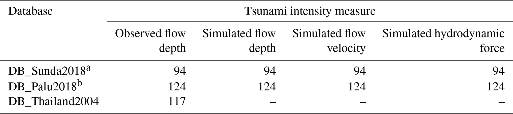
A post-tsunami database has been established for the Sunda Strait area by Syamsidik et al. (2019), Palu Bay by Paulik et al. (2019), and Khao Lak–Phuket by Ruangrassamee et al. (2006) and Foytong and Ruangrassamee (2007) in urban areas strongly affected by these events. These databases include 98, 371, and 120 observed flow depth traces at buildings, respectively. Here, the tsunami fragility analysis stands on subsets of the original databases of the 2018 Sunda Strait, 2018 Sulawesi–Palu, and 2004 Indian Ocean (Khao Lak–Phuket) tsunamis, as explained in Sects. 3.2.2, 3.2.3, and 2.2, respectively. We define these subsets as “new” databases, and we call them DB_Sunda2018, DB_Palu2008, and DB_Thailand2004, respectively. We note that the use of smaller databases for the fragility assessment is expected to increase the uncertainty in the exact shape of the fragility curves. Each database gathers exclusive information regarding the degree of damage, the building characteristics, and the flow depth traces (Tables 1 and 2). A brief analysis of the key variables (i.e., damage scale, building class, and tsunami intensity) are presented below.

Table 1Harmonization between the different damage scales used in DB_Sunda2018, DB_Palu2018, and DB_Thailand2004.

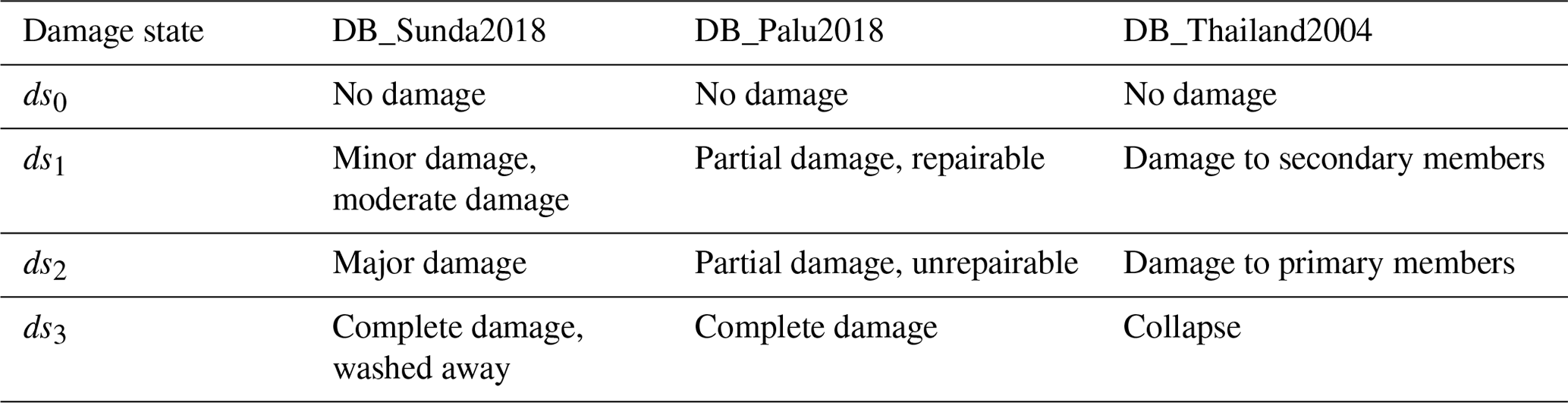
Download Print Version | Download XLSX

2.1 Damage state

Each field survey adopted a different scale to record the degree of structural damage. In DB_Sunda2018, the five-state damage scale proposed by Macabuag et al. (2016) and Suppasri et al. (2020) is adopted, ranging from no damage to complete damage or washed away. In DB_Palu2018, the observed damage was classified into four states: no damage, partial damage repairable, partial damage unrepairable, and complete damage, as proposed by Paulik et al. (2019). Finally, in DB_Thailand2004, a four-state damage scale is defined by Ruangrassamee et al. (2006). To simplify the comparison between the fragility curves, a harmonization of damage scales is proposed (Table 1). In this study, a four-state damage scale ranging from ds₀ to ds₃ is used.

2.2 Building characteristics

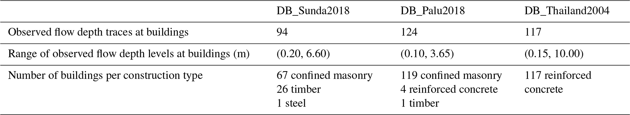
Each survey also recorded the building construction type, which influences the damage probability (Suppasri et al., 2013). In Table 2, among the 94 buildings included in DB_Sunda2018, 67 are confined masonry, 26 are timber, and 1 is a steel frame building. In DB_Palu2018, most of the buildings are confined masonry with unreinforced clay bricks (∼95 %). The database also includes reinforced concrete and timber buildings. Finally, DB_Thailand2004 contains only reinforced concrete buildings. We note that after the 2004 IOT, 120 flow depth traces were recorded at reinforced concrete structures (e.g., residence, hotel, school, shop, bridge) in the Khao Lak–Phuket area. As we are not considering the data regarding the surveyed bridges, DB_Thailand2004 includes only 117 reinforced concrete buildings.

2.3 Tsunami intensity

The tsunami intensity has been measured in terms of flow depth level. Table 2 also presents the number of flow depth traces at surveyed buildings and the range of flow depth levels for each database.

Table 2Observed flow depth traces at buildings, range of flow depth levels, and building characteristics in DB_Sunda2018, DB_Palu2018, and DB_Thailand2004.

Download Print Version | Download XLSX

3 Tsunami intensity simulations

3.1 Tsunami numerical modelling with a landslide source

3.1.1 Tsunami inundation model

The TUNAMI two-layer tsunami model used in the Sunda Strait and Palu areas relies on a two-layer numerical model solving non-linear shallow water equations. It considers two interfacing layers and appropriate kinematic and dynamic boundary conditions at the seafloor, interface, and water surface (Imamura and Imteaz, 1995; Pakoksung et al., 2019). To reproduce the landslide-generated tsunami, we model the interactions between tsunami generation and submarine landslides as upper and lower layers. The mathematical model performed in the landslide-tsunami code is obtained from a stratified medium with two layers. The first layer, composed of a homogeneous inviscid fluid with constant density, ρ₁, represents the seawater, and the second layer is composed of a fluidized granular material with a density, ρ_s, and porosity, φ. As assumed by Macías et al. (2015), the mean density of the fluidized sliding mass is constant and equals $ρ_{2} = (1 - φ) ρ_{s} + φ ρ_{1}$ . We consider the two layers immiscible. The governing equations are written as follows.

The continuity equation of the seawater (first layer) is

\begin{matrix} (1) & \frac{\partial Z_{1}}{\partial t} + \frac{\partial Q_{1 x}}{\partial x} + \frac{\partial Q_{1 y}}{\partial y} = 0 . \end{matrix}

The momentum equations of the seawater in the x and y directions are

\begin{array}{l} \frac{\partial Q_{1 x}}{\partial t} & + \frac{\partial}{\partial x} (\frac{Q_{1 x}^{2}}{D_{1}}) + \frac{\partial}{\partial y} (\frac{Q_{1 x} Q_{1 y}}{D_{1}}) \\ (2) & + g D_{1} \frac{\partial Z_{1}}{\partial x} + g D_{1} \frac{\partial Z_{2}}{\partial x} + τ_{1 x} = 0, \\ \frac{\partial Q_{1 y}}{\partial t} & + \frac{\partial}{\partial x} (\frac{Q_{1 x} Q_{1 y}}{D_{1}}) + \frac{\partial}{\partial y} (\frac{Q_{1 y}^{2}}{D_{1}}) \\ (3) & + g D_{1} \frac{\partial Z_{1}}{\partial y} + g D_{1} \frac{\partial Z_{2}}{\partial y} + τ_{1 y} = 0 . \end{array}

The continuity equation of the landslide (second layer) is

\begin{matrix} (4) & \frac{\partial Z_{2}}{\partial t} + \frac{\partial Q_{2 x}}{\partial x} + \frac{\partial Q_{2 y}}{\partial y} = 0 . \end{matrix}

The momentum equations of the landslide in the x and y directions are

\begin{array}{l} \frac{\partial Q_{2 x}}{\partial t} & + \frac{\partial}{\partial x} (\frac{Q_{2 x}^{2}}{D_{2}}) + \frac{\partial}{\partial y} (\frac{Q_{2 x} Q_{2 y}}{D_{2}}) \\ (5) & + g D_{2} \frac{\partial Z_{2}}{\partial x} + g D_{2} \frac{ρ_{1}}{ρ_{2}} \frac{\partial Z_{1}}{\partial x} + τ_{2 x} = 0, \\ \frac{\partial Q_{2 y}}{\partial t} & + \frac{\partial}{\partial x} (\frac{Q_{2 x} Q_{2 y}}{D_{2}}) + \frac{\partial}{\partial y} (\frac{Q_{2 y}^{2}}{D_{2}}) \\ (6) & + g D_{2} \frac{\partial Z_{2}}{\partial y} + g D_{2} \frac{ρ_{1}}{ρ_{2}} \frac{\partial Z_{1}}{\partial y} + τ_{2 y} = 0 . \end{array}

Index 1 and 2 refer to the first and the second layers, respectively, and ρ₁ and ρ₂ are the densities of the seawater and the landslide. $Z_{i} (x, y, t)$ , $Q_{i} (x, y, t)$ , and $τ_{i} (x, y, t)$ represent the level of the layer based on the mean water level, the vertically integrated discharge, and the bottom stress in each layer at each point (x,y) over the time t, respectively (Fig. A1). D_i denotes the thickness of each layer. The fifth term of the momentum equations (Eqs. 2, 3, 5, and 6) represents the interaction between the two layers. The tsunami model provides the maximum water flow depth and flow velocity along the coast during the tsunami inundation. The hydrodynamic force acting on buildings and infrastructure is defined as the drag force per unit width of the structure, as shown in Eq. (7) (Koshimura et al., 2009b).

\begin{matrix} (7) & F = \frac{1}{2} C_{D} ρ u^{2} D \end{matrix}

C_D represents the drag coefficient (C_D=1.0 for simplicity), ρ is the seawater density ( $ρ = 1000 kg m^{- 3}$ ), u stands for the current velocity (m s⁻¹), and D is the inundation depth (m).

3.1.2 Flow resistance within a tsunami inundation area

BATNAS and DEMNAS, Indonesia, provided the bathymetric and topographic data at 180 and 8 m resolutions, respectively. The data were established from synthetic aperture radar (SAR) images (http://tides.big.go.id/DEMNAS/index.html, last access: 2 February 2020). Both datasets were resampled to three computational domains with a grid size of 20 m resolution (Fig. 2a and b). In Palu City, the bathymetric and topographic data at 1 m resolution were obtained through lidar images and supplied by the Geospatial Information Agency (BIG), Indonesia (Fig. 2c and d).

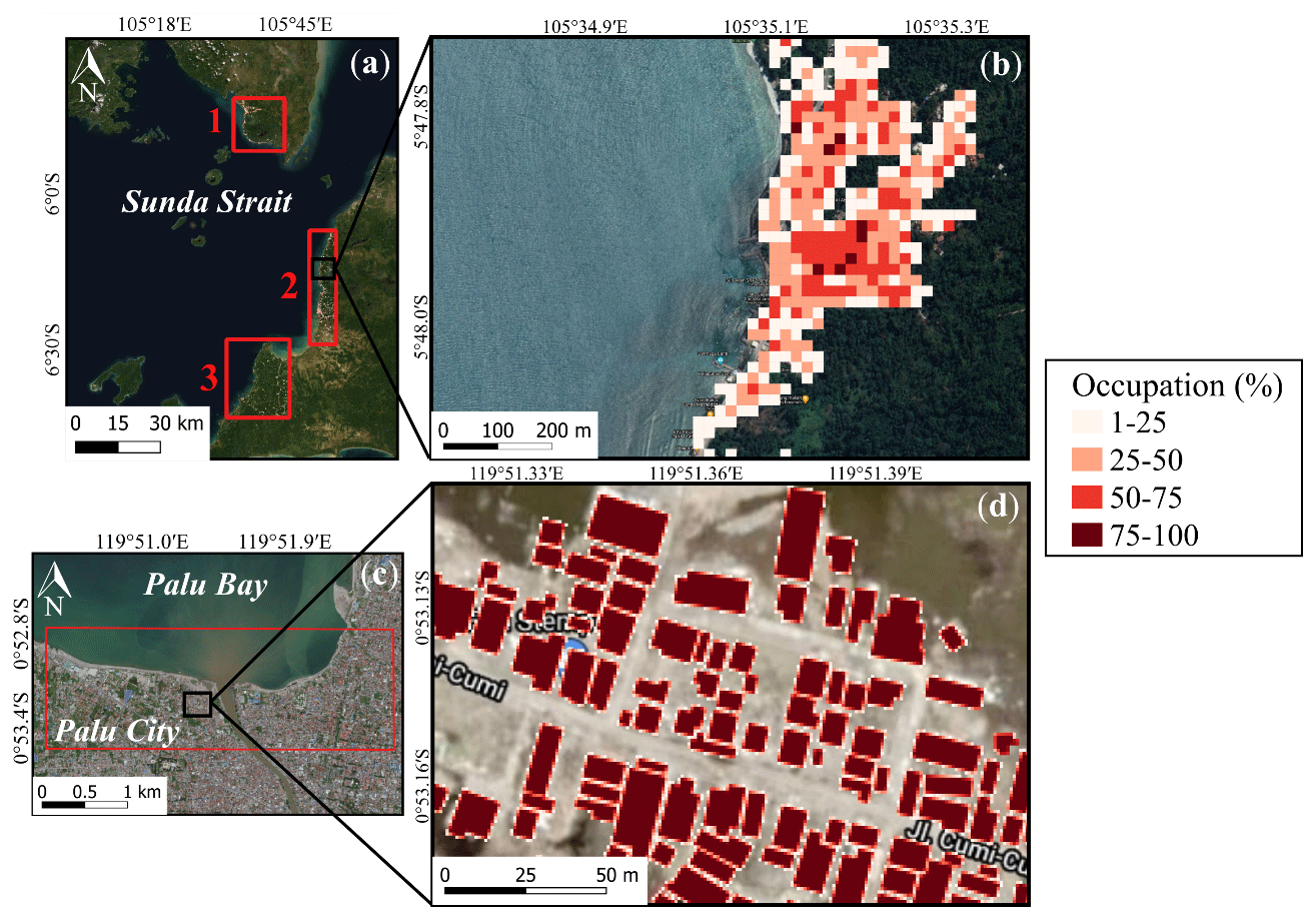
https://nhess.copernicus.org/articles/21/2313/2021/nhess-21-2313-2021-f02

Figure 2(a and c) Computational areas in the Sunda Strait (1–3) and Palu City, and (b and d) magnified view of the building occupation ratio in Sunda Strait (20 m resolution) and Palu City (1 m resolution) (background ESRI and © Google Maps).

For tsunami inundation modelling in a densely populated area, we apply a resistance law with the composite equivalent roughness coefficient depending on the land use and building conditions, as shown in Eq. (8) (Aburaya and Imamura, 2002; Koshimura et al., 2009a).

\begin{matrix} (8) & n = \sqrt{n_{0}^{2} + \frac{C_{D}}{2 g d} * \frac{θ}{100 - θ} * D^{4 / 3}}, \end{matrix}

where n_o corresponds to the Manning's roughness coefficient (n_o=0.025 $s m^{- 1 / 3}$ ), C_D represents the drag coefficient (C_D=1.5; Federal Emergency Management Agency (FEMA), 2003), and the constant d signifies the horizontal scale of buildings (∼15 m). θ is the building occupation ratio in percent (0 %–100 %) for each computational cell of 20 m×20 m and 1 m×1 m resolutions in Sunda Strait and Palu areas, respectively. θ is obtained by computing the building area over each pixel using geographic information system (GIS) data. The computational cell corresponding to buildings can be inundated by the n Manning coefficient through the term D, which represents the simulated flow depth (m). In the urban areas of Sunda Strait and Palu, the average occupation ratios are 24 % and 84 %, respectively (Fig. 2b and d). In non-residential areas, we set the Manning's roughness coefficients inland and on the seafloor to 0.03 and 0.025, respectively, which are typical values for vegetated and shallow water areas (Kotani, 1998).

3.2 Calibration and validation of the tsunami inundation model

3.2.1 Performance parameters

The tsunami inundation model is calibrated using two performances parameters: K and κ proposed by AIDA (1978), as defined below:

\begin{matrix} (9) & \log K = \frac{1}{n} \sum_{i = 1}^{n} \log K_{i}, \end{matrix}

\begin{array}{l} (10) & \log κ = \sqrt{\frac{1}{n} \sum_{i = 1}^{n} (\log K_{i})^{2} - (\log K)^{2}}, \\ (11) & K_{i} = \frac{x_{i}}{y_{i}}, \end{array}

where x_i and y_i are the recorded and simulated tsunami flow depths at location i. K is defined as the geometrical mean of K_i, and κ is defined as deviation or variance from K. The Japan Society of Civil Engineers (JSCE) (2002) recommends $0.95 < K < 1.05$ and κ<1.45 for the model results to achieve “good agreement” in the tsunami source model and propagation and inundation model evaluation (Otake et al., 2020; Pakoksung et al., 2018).

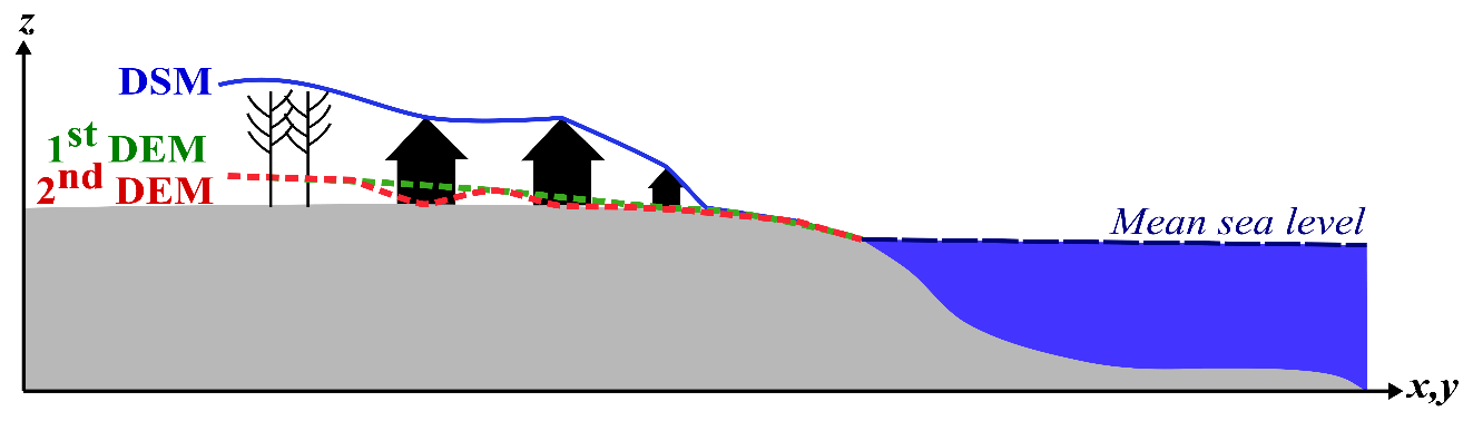
https://nhess.copernicus.org/articles/21/2313/2021/nhess-21-2313-2021-f03

Figure 3Topographic corrections performed on the DSM and the 1st DEM. The 2nd DEM is used as new topography in the TUNAMI two-layer model.

Download

https://nhess.copernicus.org/articles/21/2313/2021/nhess-21-2313-2021-f04

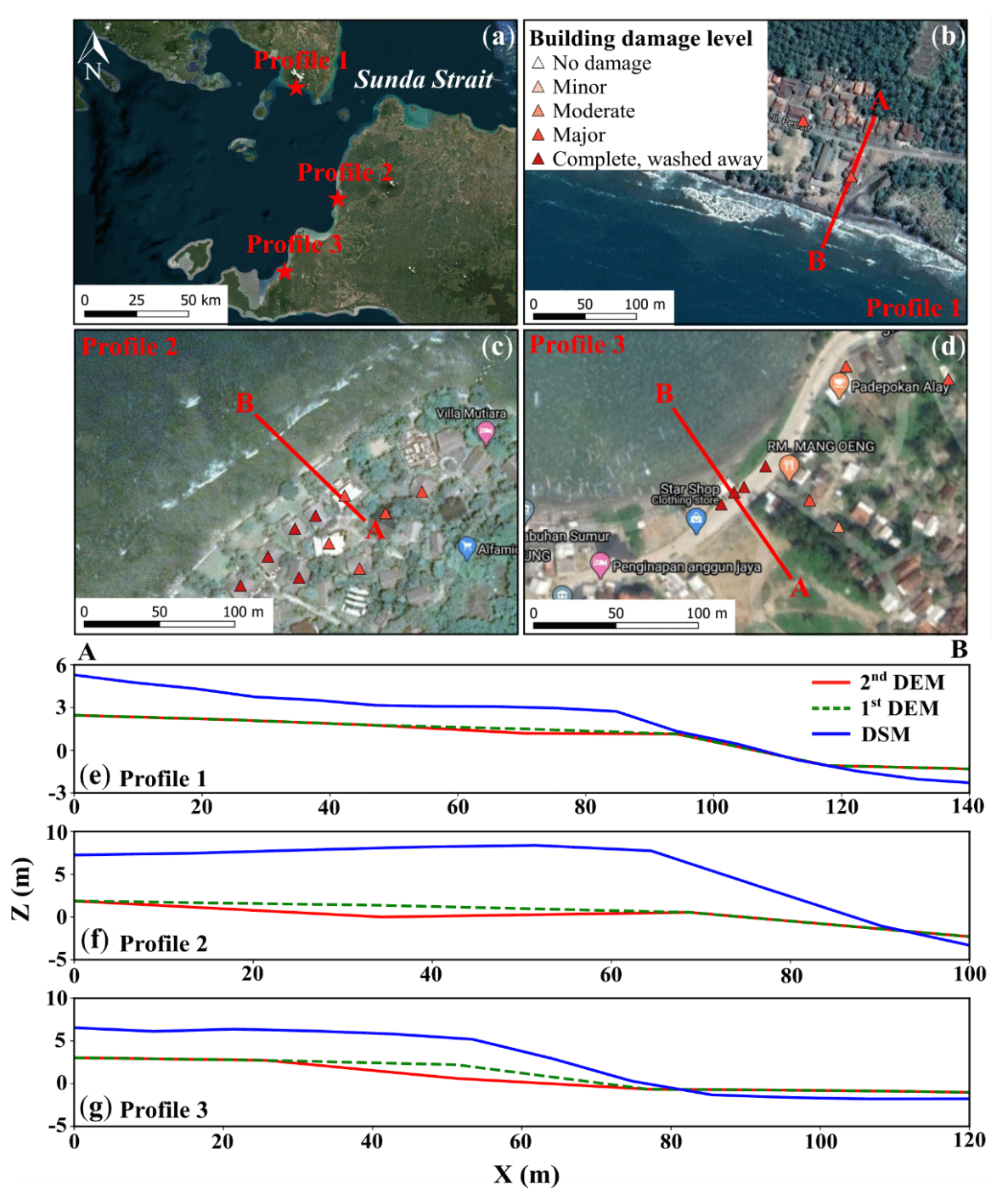
Figure 4(a) Cross sections along Sunda Strait coasts. One cross section is realized in the computational areas (b and e) 1, (c and f) 2, and (d and g) 3 to illustrate the topographic corrections applied to the DSM at buildings using QGIS (a triangle represents a building) (background ESRI and © Google Maps).

3.2.2 The 2018 Sunda Strait tsunami inundation model

To correct the digital surface model (DSM), we removed the vegetation, building, and infrastructure elevations based on the linear smoothing method and used the resulting digital elevation model (1st DEM) as topography in the tsunami inundation model (Fig. 3). The vertical accuracy of the DSM and DEM is about 4 m. The 2018 Sunda Strait tsunami model depends on the density of the landslide (ρ₂), its stable slope (α), its volume (V_L), and its sliding time (t_S). As proposed by Paris et al. (2020), the low sensitivity parameters are set as follows: $ρ_{2} = 1500 kg m^{- 3}$ , $α = 5^{\circ}$ , and V_S=0.15 km³. We reach the best fit between the simulated and observed flow depths at buildings for 10 min sliding time. Nevertheless, most of the simulated flow depths are underestimated compared to the observed ones, with a mean difference of 0.28±1 m. Using quantum GIS (QGIS) software, we smoothed the 1st DEM to remove these mean differences in elevation at buildings where the flow depth is underestimated. The resulting DEM (2nd DEM) provides a topography more reliable at buildings (Fig. 3). We completed three cross sections along the Sunda Strait coasts to show the different corrections applied to the DSM (Fig. 4a–g). K and κ values for damaged buildings are 0.99 and 1.11, respectively, which means that we achieve “good agreement” for the Sunda Strait tsunami model, displayed in Fig. 5a–f. We note that the simulated inundation zone overlays 94 buildings out of 98. In Sect. 4.1, the Sunda Strait tsunami fragility assessment is based on these 94 buildings (DB_Sunda2018). Simulation snapshots of the Sunda Strait tsunami propagation are shown in Fig. B1 10, 20, 60, and 120 s after the tsunami generation. In Fig. B2, the simulated tsunami height based on the best-fitting parameters is also displayed. Figure B3 illustrates the maximum simulated flow velocity of the 2018 Sunda Strait tsunami inundation model.

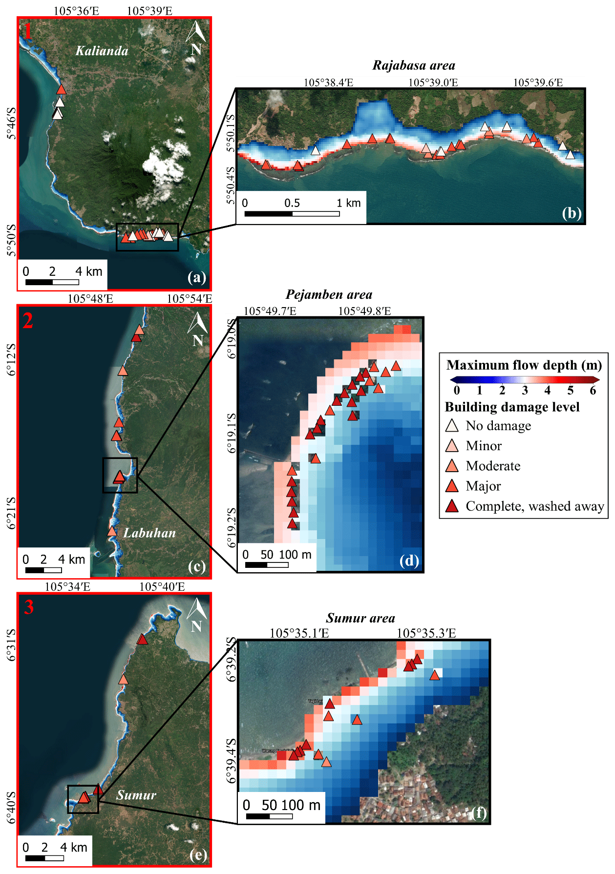
https://nhess.copernicus.org/articles/21/2313/2021/nhess-21-2313-2021-f05

Figure 5(a, c, and e) Sunda Strait final tsunami inundation model with the maximum simulated flow depth overlaid on the damaged building data in the computational areas 1 to 3, and (b, d, and f) magnified views of the maximum simulated flow depth in the Rajabasa, Pejamben, and Sumur areas (background ESRI and © Google Maps).

3.2.3 The 2018 Sulawesi–Palu tsunami inundation model

We increased the mean sea level (MSL) by 2.3 m to reproduce the high tide during the 2018 Sulawesi–Palu tsunami. As shown by Pakoksung et al. (2019), the observed waveform at Pantoloan tidal gauge does not fit the simulated one with the finite fault model of TUNAMI-N2. Although recent studies show that seismic seafloor deformation may be the primary cause of the tsunami (Gusman et al., 2019; Ulrich et al., 2019), in this study, the main assumption is that the 2018 Sulawesi–Palu event was triggered by subaerial and submarine landslides. According to Heidarzadeh et al. (2019), a large landslide to the north or the south of Pantoloan tidal gauge is responsible for the significant height wave recorded. Arikawa et al. (2018) also identified several sites of potential subsidence in the northern part of Palu Bay. Based on these previous studies, we assume two large landslides: L1 and L2. Small landslides (S1–S12) also occurred in the bay; their location is known from observations from satellite imagery, field surveys, and video footage (Arikawa et al., 2018; Carvajal et al., 2019) (Fig. 6). From the trial and error method and the topographic and bathymetric data provided by the Geospatial Information Agency (BIG), we determined the soil property and achieved the volume of the landslides (Table 3). In Fig. 7, the submarine landslides model reproduces well the tsunami observations at Pantoloan.

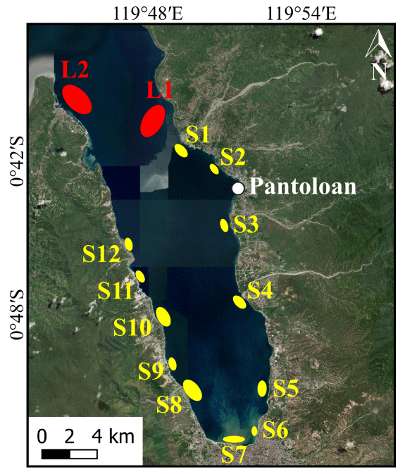
https://nhess.copernicus.org/articles/21/2313/2021/nhess-21-2313-2021-f06

Figure 6Location of the hypothesized landslides (S: small; L: large) in Palu Bay (background ESRI).

Table 3Hypothesized landslide parameters (location and volume) in Palu Bay.

^a Based on our assumption from Arikawa et al. (2018) and Heidarzadeh et al. (2019). ^b Based on observations from satellite imagery, field surveys, and video footage (Arikawa et al., 2018; Carvajal et al., 2019).

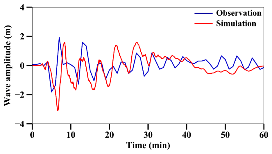
Download Print Version | Download XLSX

https://nhess.copernicus.org/articles/21/2313/2021/nhess-21-2313-2021-f07

Figure 7Comparison between observed and simulated wave heights at Pantoloan tidal gauge in Palu Bay, Sulawesi, Indonesia.

Download

The calibration of the model depends on the landslide S8 because (i) as a small landslide, its volume is too small to distort the simulated wave height at the Pantoloan tidal gauge, (ii) it has the largest volume among the other small landslides, and (iii) it is close and ideally oriented to Palu City; the slide direction, captured by an aircraft pilot, is perpendicular to the bay (Carvajal et al., 2019). The density of the landslides (ρ₂), their stable slope (α), and their sliding time (t_s) are set as follows: ρ₂=2000 kg m⁻³ (Palu Bay receives a large amount of fine continental deposits such as clay-sized sediments; Frederik et al., 2019), $α = 14^{\circ}$ (Chakrabarti, 2005), and t_S=10 min. For a landslide ratio of 1.2 (i.e., S8 volume is multiplied by 1.2), the tsunami model shows a great similarity between observed and simulated flow depths (a=1.027). The simulated tsunami inundation zone overlays 175 traces out of 371 because (i) 151 buildings with flow depth traces are not included in our computational area (Fig. 2c) and (ii) 45 buildings are outside the simulated tsunami envelope, which is shorter than the surveyed one (Fig. 8). The geometric mean is near the recommended values (K=0.93), while the standard deviation and the root mean square error (RMSE) are high (κ=2.18, RMSE=0.92 m). Therefore, to develop accurate and reliable curves, we set a 1 m confidence interval including 124 flow depth traces at buildings out of 175 (Fig. 9). In Sect. 4.2, the Sulawesi–Palu tsunami fragility assessment is based on these 124 buildings (DB_Palu2018). K and κ values for damaged buildings are 0.93 and 2.14, respectively, with a root mean square error of 0.26 m. The validity of the model is mainly based on the geometric mean K, close to 0.95, so we consider the tsunami inundation model accurate enough (Fig. 8). In Fig. C1, the simulation snapshots of the Sulawesi–Palu tsunami propagation are shown 2, 10, 30, and 60 s after the tsunami generation. The simulated tsunami height based on the best-fitting parameters is also displayed in Fig. C2. Figure C3 illustrates the maximum simulated flow velocity of the 2018 Sulawesi–Palu tsunami inundation model.

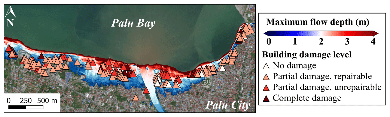
https://nhess.copernicus.org/articles/21/2313/2021/nhess-21-2313-2021-f08

Figure 8Sulawesi–Palu final tsunami inundation model with the maximum simulated flow depth overlaid on the damaged building data (background ESRI).

https://nhess.copernicus.org/articles/21/2313/2021/nhess-21-2313-2021-f09

Figure 9Comparison between observed and simulated flow depths at damaged building for an S8 ratio of 1.2; a confidence interval is set at 1 m flow depth.

Download

4 Tsunami fragility assessment

The proposed fragility assessment framework has two main steps. In the first step, an exploratory analysis aims to (i) assess the trends that the available data follow and (ii) determine the main explanatory variables that need to be included in the statistical model and their influence on the slope and intercept of the fragility curves. Then, we select a statistical model and examine its goodness-of-fit to the data based on the observations of the exploratory analysis. We note that the development of the computed fragility curves for the 2018 Sunda Strait and 2018 Sulawesi–Palu tsunamis is directly based on DB_Sunda2018 and DB_Palu2018, in which each building has both observed and simulated flow depth values (Table 4).

Table 4Number of buildings used for the tsunami fragility analysis of the 2018 Sunda Strait, 2018 Sulawesi–Palu, and 2004 IOT (Khao Lak–Phuket) events.

^a Surveyed buildings included in the Sunda Strait simulated tsunami inundation zone. ^b Surveyed buildings included in the Palu simulated tsunami inundation zone and in the 1 m confidence interval.

Download Print Version | Download XLSX

To explore the relationship between the tsunami intensity and the probability of damage, we fit a generalized linear model (GLM) to the data of each database, as proposed by the GEM guidelines (Rossetto et al., 2014). A GLM assumes that the response variable y_ij is assigned 1 if the building j sustained damage DS≥ds_i and 0 otherwise. The variable follows a Bernoulli distribution:

\begin{matrix} (12) & y_{i j} \sim Bernoulli (π_{i} ({\tilde{x}}_{j})), \end{matrix}

where $π_{i} ({\tilde{x}}_{j})$ is the probability that a building j will reach or exceed the “true” damage state ds_i given estimated tsunami intensity level ${\tilde{x}}_{j}$ . The Bernoulli distribution is characterized by its mean,

\begin{matrix} (13) & μ_{i j} = π_{i} ({\tilde{x}}_{j}), \end{matrix}

which is expressed here in terms of a probit model, commonly used to express the mean in the empirical fragility assessment field (Rossetto et al., 2013), defined in terms of Φ[.], the cumulative distribution function of a standard normal distribution:

\begin{matrix} (14) & Φ^{- 1} [π_{i} ({\tilde{x}}_{j})] = η_{i j}, \end{matrix}

where η_ij is the linear predictor, which can be written in the form

\begin{matrix} (15) & η_{i j} = θ_{0 i} + θ_{1 i} \ln ({\tilde{x}}_{j}), \end{matrix}

where θ_1i and θ_0i are the two regression coefficients representing the slope and the intercept, respectively, of the fragility curve corresponding to damage state ds_i. For the exploratory analysis, the tsunami intensity is measured in terms of observed flow depth levels. We also fit the GLM models to subsets of data of each database to explore the importance of the construction type to the shape of the fragility curves. The confidence in the exact shape of the mean curves is estimated and presented in terms of the 90 % confidence intervals around the best-estimate curves.

Based on the aforementioned observations, we construct parametric statistical models for the three databases to (i) identify the simulated tsunami measure type that fits the data best and (ii) construct fragility curves for the tsunami intensity type that fits the data best.

Ideally, the response variable y_ij of an appropriate statistical model is the damage state $i = {0, 1, 2, 3}$ sustained by a building j. The damage state follows a categorical distribution (i.e. also called a generalized Bernoulli distribution) which describes the possible levels of damage $i = {0, 1, 2, 3}$ sustained by a given building (Table 1). The random component of this model can be written as

\begin{matrix} (16) & y_{i j} \sim Categorical (P (DS = {ds}_{i} | {\tilde{x}}_{j})), \end{matrix}

where $P (DS = {ds}_{i} | {\tilde{x}}_{j})$ is the probability that a building j will reach the “true” damage state ds_i given estimated tsunami intensity level ${\tilde{x}}_{j}$ .

\begin{matrix} (17) & P (DS = {ds}_{i} | {\tilde{x}}_{j}) = \{\begin{cases} 1 - π_{i} ({\tilde{x}}_{j}), & i = 0 \\ π_{i} ({\tilde{x}}_{j}) - π_{i + 1} ({\tilde{x}}_{j}), & 0 < i < i_{max} \\ π_{i} ({\tilde{x}}_{j}), & i = i_{max} \end{cases} \end{matrix}

Multiple expressions of the systematic component are constructed to test their goodness of fit. With regard to the link function, apart from the commonly used probit function, two alternative expressions found in the GEM guidelines for empirical vulnerability assessment (Rossetto et al., 2013), namely the logit and complementary loglog (termed here “cloglog”), are considered in the form

\begin{matrix} (18) & η_{i j} = \{\begin{cases} Φ^{- 1} [π_{i} ({\tilde{x}}_{j})], & probit \\ \ln (\frac{π_{i} ({\tilde{x}}_{j})}{1 - π_{i} ({\tilde{x}}_{j})}), & logit \\ \ln (- \ln (1 - π_{i} ({\tilde{x}}_{j}))), & cloglog \end{cases} . \end{matrix}

The linear predictor is also expressed in various forms of increasing complexity, as depicted in Eq. (19).

η_{i j} = \{\begin{array}{lr} θ_{0} + θ_{1} {\tilde{x}}_{j} & (19a) \\ θ_{0} + θ_{1 i} {\tilde{x}}_{j} & (19b) \\ θ_{0} + θ_{1} {\tilde{x}}_{j} + θ_{2} class & (19c) \\ θ_{0} + θ_{1 i} {\tilde{x}}_{j} + θ_{2} class & (19d) \\ θ_{0} + θ_{1} {\tilde{x}}_{j} + θ_{2} class + θ_{3} {\tilde{x}}_{j} class & (19e) \end{array}

Class is a categorical unordered variable which expresses here the construction type. θ₀₋₃ are the unknown regression coefficients of the model. Equations (19a) and (19b) assume that the fragility curves are only influenced by the tsunami intensity. Equation (19a) assumes that the slope of the fragility curves is the same for all damage states. In contrast, Eq. (19b) allows the slope of each curve to vary for each damage state; the slope varies for each fragility curve. The following three equations account for the influence of the building class (i.e. the construction type) in the shape of the fragility curves. All three equations assume that the construction type affects the intercept of the fragility curves, and only Eq. (19e) assumes that the construction type affects both the intercept and the slope of the curves. Finally, Eqs. (19c) and (19e) assume identical slopes for all fragility curves irrespective of the damage state. In contrast, Eq. (19d) relaxes this assumption and considers that the slope changes for each damage state. The combinations of random and systematic components result in five distinct models (Table 5).

Table 5Statistical models examined for each database.

Download Print Version | Download XLSX

https://nhess.copernicus.org/articles/21/2313/2021/nhess-21-2313-2021-f10

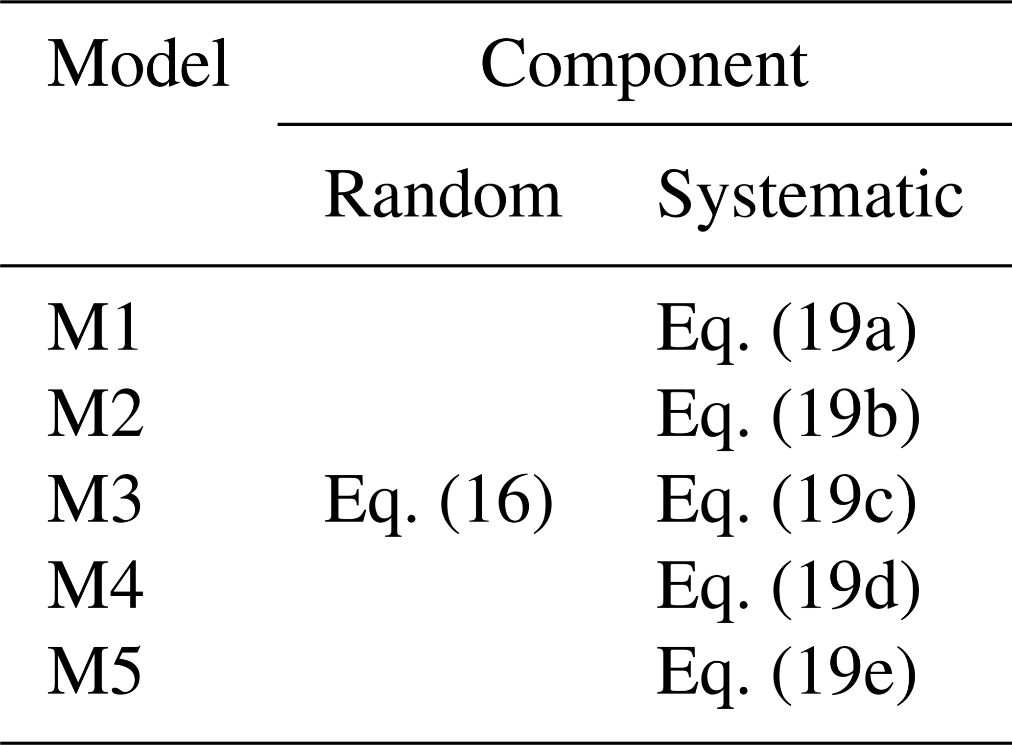
Figure 10Probit functions fitted for each individual damage state to DB_Sunda2018 (a) to assess whether the observed flow depth is an efficient descriptor of damage and (b) to assess whether the construction type affected the shape of fragility curves for ds₂ and ds₃. In both cases, the 90 % confidence interval is plotted.

Download

In what follows, we fit multiple models to each database based on the observations of the exploratory analysis. We examine the goodness of fit of these models for a given tsunami intensity measure and link function with two formal tests, as proposed in the GEM guidelines (Rossetto et al., 2014). Firstly, we compare the Akaike information criterion (AIC) values, which estimates the prediction error of the examined models (Akaike, 1974). The model with the lowest value fits the data best. The alternative models used in this study are nested, which means that the more complex model includes all the terms of the simpler ones plus an additional term. For this reason, we also perform a series of likelihood ratio tests to examine whether the fit provided by the model with the lowest AIC value is statistically significant over its alternative nested models, which relaxes its assumptions (Rossetto et al., 2014). We also use the AIC value to determine which of these simulated intensity measures fits the data best. Furthermore, the 90 % confidence intervals of the best-estimate fragility curves are constructed using bootstrap analysis. According to the latter analysis, 1000 samples of the database are obtained with a replacement, and the selected model is refitted to each sample.

4.1 DB_Sunda2018

We fit the GLM models to the data in DB_Sunda2018 (irrespective of their structural characteristics), and we plot the obtained probit functions against the natural logarithm of the observed flow depth to explore how the slope and the intercept of the models change for each damage state (Fig. 10a). The 90 % confidence intervals around the best-estimate curves are also included. All three curves have positive slopes, which indicates that the flow depth is an adequate descriptor of the damage caused by a tsunami as the probability of a given damage state being reached or exceeded increases with the increase in the flow depth. The slope of each function is similar for ds₂ and ds₃ and different for ds₁. Nonetheless, the curve corresponding to ds₁ is also associated with substantial uncertainty. In Fig. 10b, we fit probit models to subsets of the available data for the two main construction types. One of the drawbacks of the small database is that not all damage states were observed for each building class. Therefore, the comparison of probit models is limited for damage states ds₂ and ds_3. The curves for the two construction types appear to be substantially different. As expected, the timber buildings are more vulnerable than the confined masonry buildings. Their intercept is responsible for the difference as the two curves are parallel. It indicates the need to develop a statistical model which allows only the intercept to change with the construction type, and the slope should be identical.

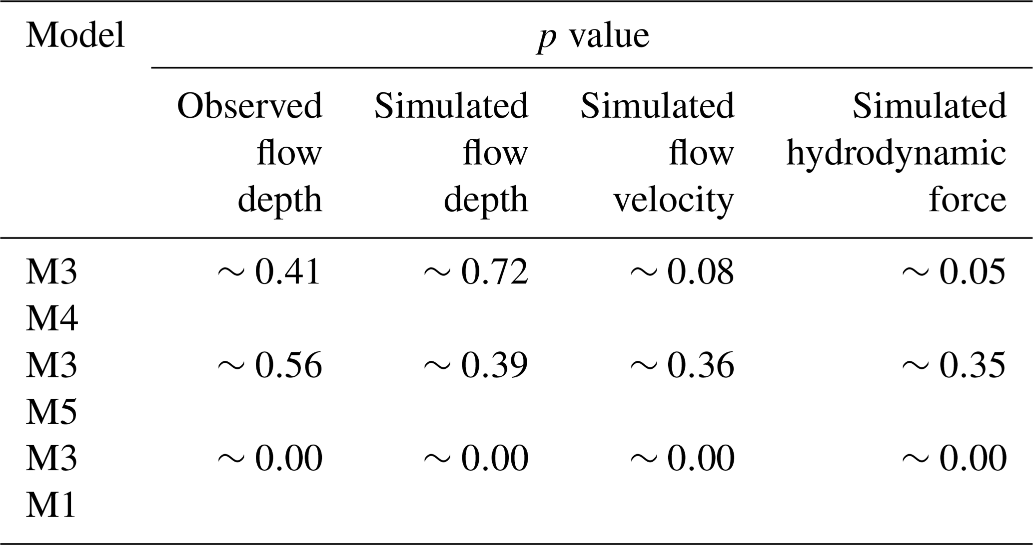
Following the main observations of the exploratory analysis, we consider that M3 is an acceptable model with two explanatory variables: the tsunami intensity and the construction type. To assess its goodness of fit, we consider each link function with three alternatives for the linear predictor (i.e., M4, M5, and M1) which relax some of its assumptions. In Table 6, we compare the AIC values of the three models to assess the fit of the different models for the observed flow depth levels assuming the probit link function. M3 has the smallest AIC value compared to its alternatives, which indicates that it fits the data better than the remaining three models. Nonetheless, some of these differences are rather small, and it raises the question of whether the improvement in the fit provided by M3 is statistically significant over its alternatives. To address this, we perform likelihood ratio tests, and the results are reported in Table 7. We note that the p values vary for the three comparisons. The p value is significantly above the 0.05 threshold when the identical slope for each fragility curve assumption (i.e. comparison of M3 and M4) is tested. This means that M4 (which assumes varying slopes for each damage state) does not provide a statistically significant improvement than its alternative. Therefore, the fit of M3 is the best. Similarly, the p value is well above the threshold for M3 vs. M5, highlighting that the construction type does not affect the slope of the fragility curves. In contrast, the p value is well below the threshold for the comparison of M3 and M1, indicating that the construction type is an important variable and affects only the intercept. Having concluded that M3 based on the observed flow depth data fits the data better than its alternatives (i.e. M4, M5, and M1), we repeat the procedure to identify which simulated intensity type fits the data best. Table 6 also shows the comparison of the AIC values for the three simulated tsunami intensity types. For all simulated intensity types, M3 is identified as the model which fits the data better than its alternatives, and this conclusion is further reinforced by the likelihood ratio tests presented in Table 7. By comparing the AIC values for M3 for all three simulated intensity types, we note that the simulated flow depth is the tsunami intensity that fits the data best. The aforementioned observations can also be made if instead of the probit link function, the two alternative functions (i.e. logit and cloglog) are considered, as depicted in Table D1. The comparison of the AIC values of M3 for the three link functions identifies the probit link function as the one that fits the data best.

The regression coefficients of the 2018 Sunda Strait fragility curves based on the best-fitted M3 model with a probit link function are listed in Table E1. An advantage of constructing a complex model that accounts for the ordinal nature of the damage and for the two main construction types in the systematic component is that fragility curves for timber buildings can be obtained even for the states for which there are available data. A timber building is found to sustain more damage than confined masonry buildings for the more intense damage states. Nonetheless, there is substantially more uncertainty in the prediction of the likelihood of damage, and this can be attributed to the rather small sample size.

Table 6AIC values for the three models assuming probit link function fitted to the observed and simulated tsunami intensity measures of DB_Sunda2018.

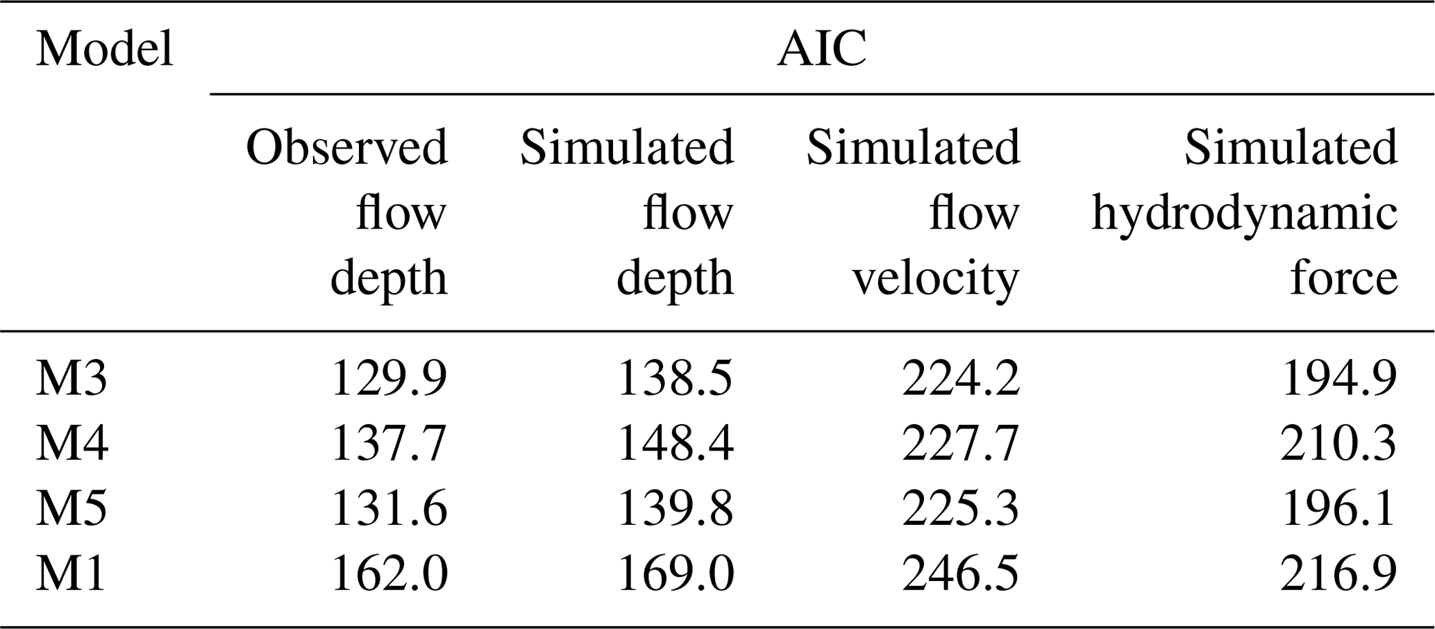
Download Print Version | Download XLSX

Table 7Likelihood ratio test summary for all available observed and simulated tsunami intensity measures of DB_Sunda2018.

Download Print Version | Download XLSX

4.2 DB_Palu2018

We also fit GLM models to the data in DB_Palu2018 using the observed tsunami flow depth to express the tsunami intensity and then to construct fragility curves and their 90 % confidence intervals for the three individual damage states (Fig. 11). The data seem to produce fragility curves with positive slopes for d_S1 and d_S2 and a negative slope for d_S3. This latter observation is counter-intuitive as it is expected that the likelihood of collapse will grow with the increase in the tsunami depth. This outcome could be attributed to the collected sample, which includes very few collapsed buildings observed at low flow depth levels.

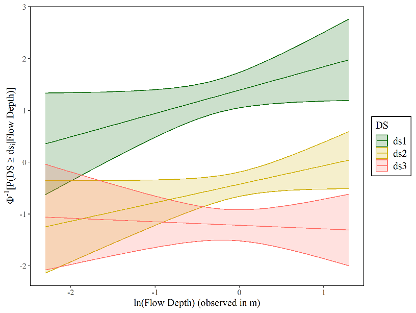
https://nhess.copernicus.org/articles/21/2313/2021/nhess-21-2313-2021-f11

Figure 11Probit functions fitted for each individual damage state to DB_Palu2018 to assess whether the observed flow depth is an efficient descriptor of damage. The 90 % confidence interval is plotted.

Download

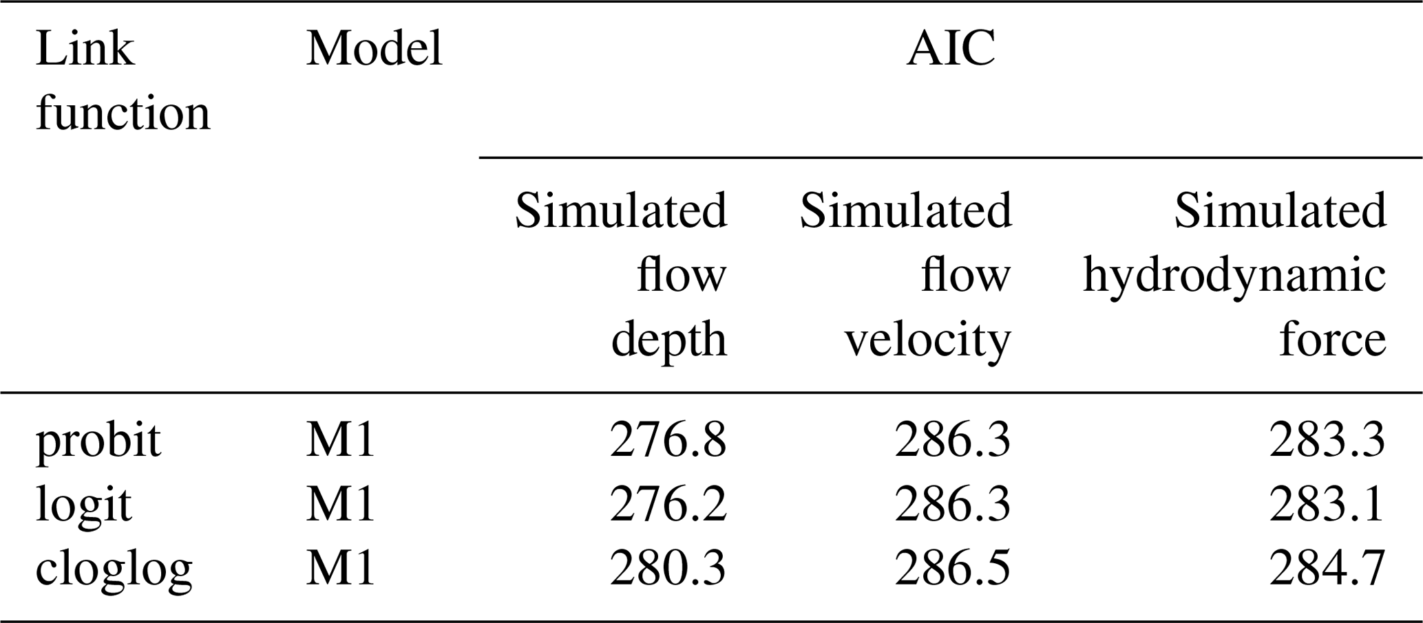
Based on the observations of the exploratory analysis, we use identical slopes for the fragility curves for all three damage states (ds₁−ds₃) to tackle the negative slope for ds₃ and three link functions. Therefore, model M1 is fitted to DB_Palu2018 assuming that the tsunami intensity is expressed in terms of simulated flow depth, flow velocity, and hydrodynamic force. Table 8 depicts the AIC values for each model. We note that for all cases the flow depth fits the data the best. Table 8 also shows that the logit function fits the data best. The regression coefficients of the 2018 Sulawesi–Palu fragility curves for the logit function are depicted in Table E2.

Table 8AIC values for model M1 fitted to the simulated tsunami intensity measures of DB_Palu2018.

Download Print Version | Download XLSX

4.3 DB_Thailand2004

The exploratory analysis aims to identify trends in the shape of the fragility curves for each damage state. Thus, we fit GLM models to DB_Thailand2004 to construct fragility curves for the three individual damage states, and we plot them with their 90 % confidence interval in Fig. 12. The data seem to produce fragility curves with positive slopes for all three damage states and also are parallel to each other, which suggests that the slope should be identical for all three curves.

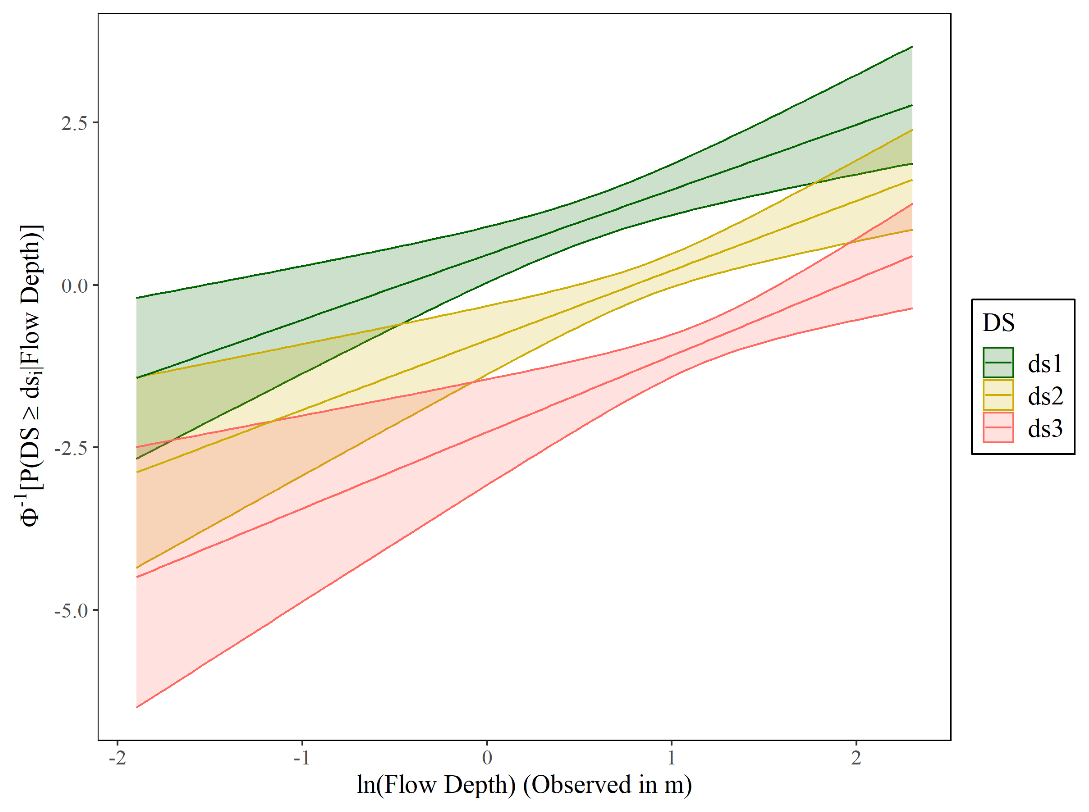
https://nhess.copernicus.org/articles/21/2313/2021/nhess-21-2313-2021-f12

Figure 12Probit functions fitted for each individual damage state to DB_Thailand2004 to assess whether the observed flow depth is an efficient descriptor of damage. The 90 % confidence interval is plotted.

Download

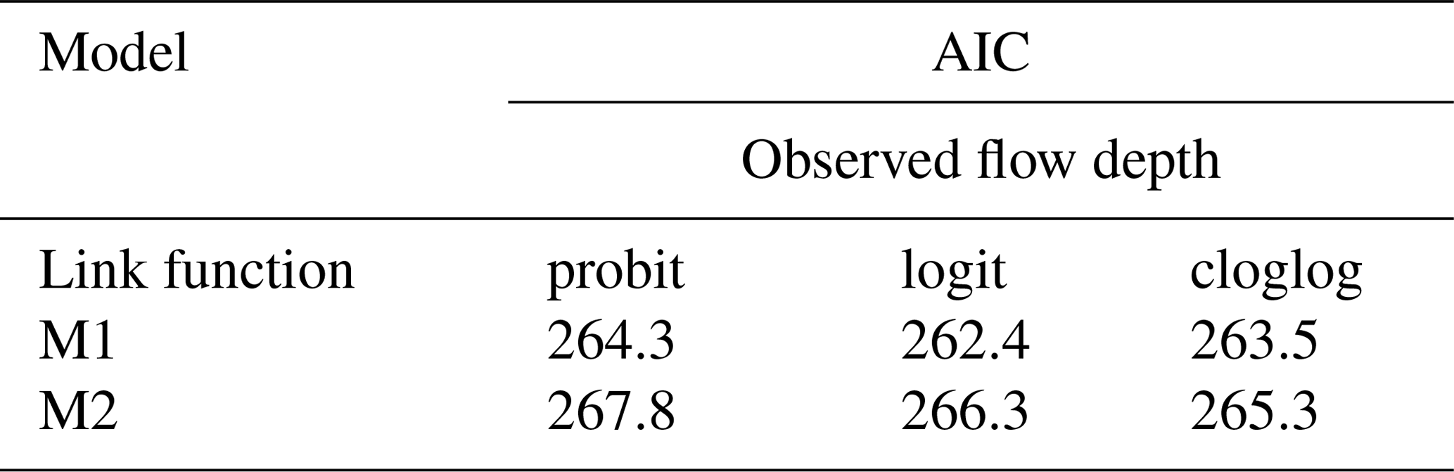
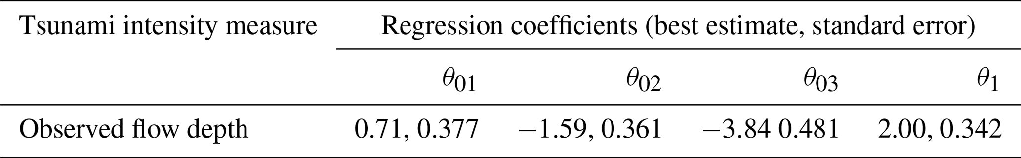
Based on the observations of the exploratory analysis, we consider model M1 as the most suitable. To test its goodness of fit, model M2, which relaxes the assumption that the slope of all three curves is identical, is also fitted to the data. In Table 9, the comparison of the AIC values for the two models also shows that M1 is the model which fits the data best for all three link functions considered in this study (i.e., probit, logit, and cloglog). We also perform a likelihood ratio test to confirm that the improvement in the fit provided by the more complex M2 model over M1 is not statistically significant. The p value is found to be equal to 0.76, 0.95, and 0.33 for the probit, logit, and cloglog functions, respectively, which is significantly above the 0.05 threshold. This suggests that M2 does not provide a statistically better fit to the data; therefore, the less complex M1 model fits the data best. The regression coefficients of the 2004 Indian Ocean (Khao Lak–Phuket) fragility curves for the best-fitted model M1 with logit link function can be found in Table E3.

Table 9AIC values for the two models fitted to the observed flow depth of DB_Thailand2004.

Download Print Version | Download XLSX

5 Results

5.1 Building fragility curves of the 2018 Sunda Strait tsunami

The fragility curves determine conditional damage probabilities according to the tsunami intensity measures of the 2018 Sunda Strait event for both confined masonry concrete (Fig. 13a–c) and timber (Fig. 14a–c) buildings of DB_Sunda2018. In Fig. 14a and b, there are no data to predict the shape of the curves between 0–1 m flow depth and 0–1 m s⁻¹ flow velocity. The curves as a function of the observed flow depth reveal a great similarity with the ones based on the simulated flow depth from the TUNAMI two-layer model (Figs. 13a and 14a). For instance, when the observed and simulated flow depths reach 3 m, the likelihood of minor to major damage (i.e., ≥ds₁, ds₂) for both timber and confined masonry buildings is approximately 99 % (Fig. 14a and b). In contrast, the likelihood of complete damage (i.e., ≥ds₃) is 70 % for timber buildings and only 10 % for confined masonry buildings. Consequently, the tsunami functions based on observation and simulation are highly similar, which illustrates the accuracy and the reliability of the tsunami inundation model. The curves show that confined masonry-type buildings have higher performance than timber structures. When the flow depth is greater than 5 m and 2.5 m, the probability of complete damage is around 99 % for confined masonry and timber buildings, respectively. We also compare the completely damaged or washed away fragility curve for confined-masonry buildings to Syamsidik et al. (2020), who developed the curve as a function of observed flow depth for these buildings, as depicted in Fig. 13a. Fragility curves representing complete damage or washed away are similar up to 4.5 m flow depth. Each curve estimates a 15 % building damage probability at 3.5 m flow depth. However, a few data points are available beyond 5 m in the Sunda Strait area. Therefore, the damage probability uncertainty is greater for this value, hence the difference between our ds₃-curve and the one produced by Syamsidik et al. (2020). The curves as functions of the maximum simulated flow velocity and the hydrodynamic force are displayed in Figs. 13b and 14b and Figs. 13c and 14c for confined masonry concrete and timber buildings, respectively.

https://nhess.copernicus.org/articles/21/2313/2021/nhess-21-2313-2021-f13

Figure 13The 2018 Sunda Strait curves for confined masonry concrete buildings. Best-estimate fragility curves, with their 90 % confidence intervals, as functions of (a) the observed and the maximum simulated flow depths, (b) the maximum simulated flow velocity, and (c) the simulated hydrodynamic force for confined masonry concrete buildings of DB_Sunda2018 sustaining minor or moderate damage (ds₁), major damage (ds₂), and complete damage or washed away (ds₃) in Sunda Strait area.

Download

https://nhess.copernicus.org/articles/21/2313/2021/nhess-21-2313-2021-f14

Figure 14The 2018 Sunda Strait curves for timber buildings. Best-estimate fragility curves, with their 90 % confidence intervals, as functions of (a) the observed and the maximum simulated flow depths, (b) the maximum simulated flow velocity, and (c) the simulated hydrodynamic force for timber buildings of DB_Sunda2018 sustaining minor or moderate damage (ds₁), major damage (ds₂), and complete damage or washed away (ds₃) in Sunda Strait area.

Download

5.2 Building fragility curves of the 2018 Sulawesi–Palu tsunami

The 2018 Sulawesi–Palu tsunami curves are developed for confined masonry buildings with unreinforced clay brick of DB_Palu2018. The computed and surveyed curves show a similar damage trend. When the observed and simulated flow depths reach 1.5 m, the building damage probabilities for partial damage repairable (i.e., ≥ds₁), partial damage unrepairable (i.e., ≥ds₂), and complete damage (i.e., ≥ds₃) are around 90 %, 40 %, and 15 %, respectively (Fig. 15a). The fragility curves based on the observed and simulated flow depths are relatively similar, especially for ds₁ and ds₃. The curves based on the flow velocity and the hydrodynamic force are displayed in Fig. 15b and c.

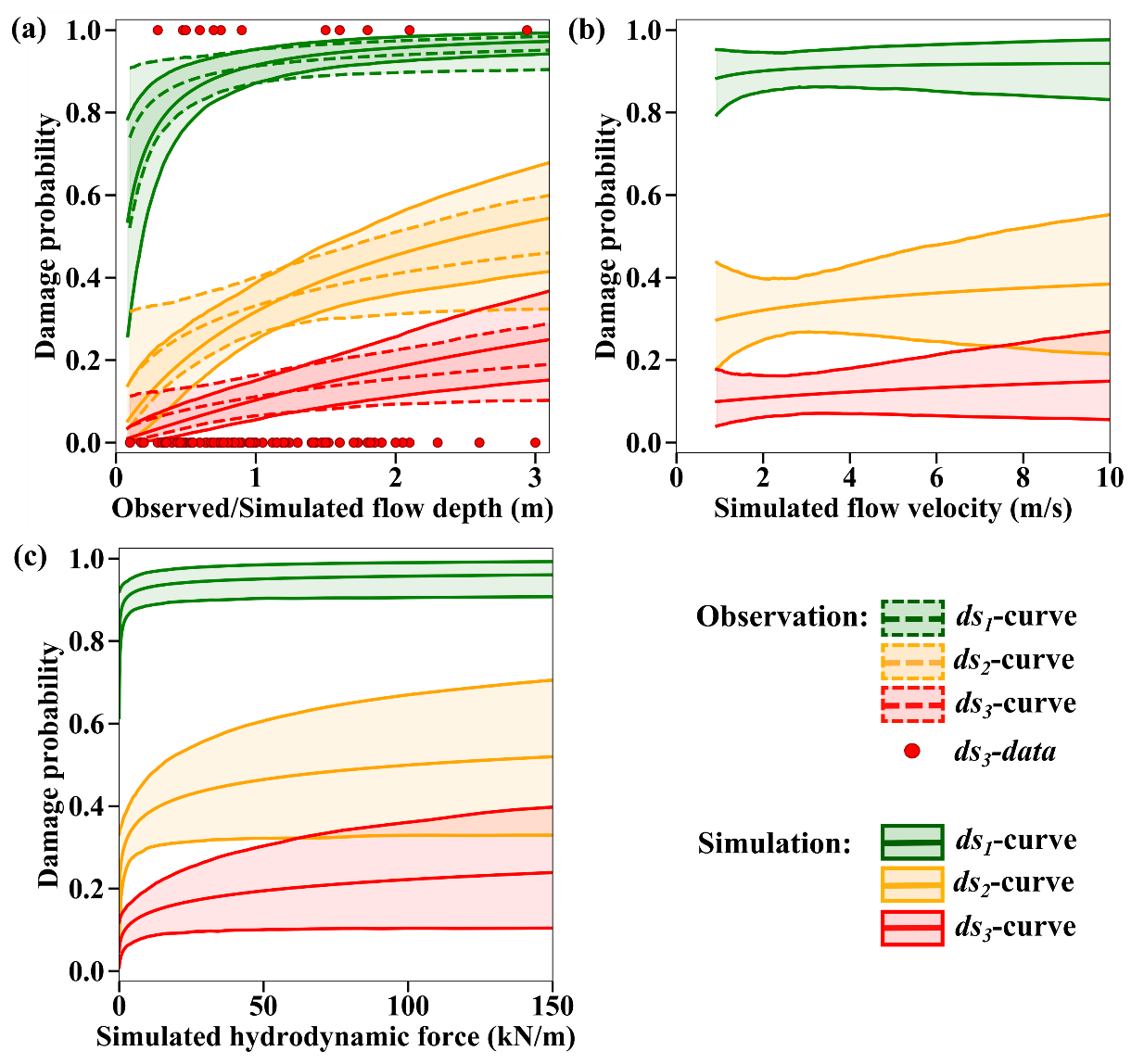
https://nhess.copernicus.org/articles/21/2313/2021/nhess-21-2313-2021-f15

Figure 15The 2018 Sulawesi–Palu curves for confined masonry buildings. Best-estimate fragility curves, with their 90 % confidence intervals, as functions of (a) the observed and the maximum simulated flow depths, (b) the maximum simulated flow velocity, and (c) the simulated hydrodynamic force for confined masonry buildings with unreinforced clay brick of DB_Palu2018 sustaining partial damage repairable (ds₁), partial damage unrepairable (ds₂), and complete damage (ds₃) in Palu City.

Download

5.3 Comparison between the 2018 and 2004 building fragility curves

In Fig. 16, we compare (i) the Sunda Strait and Sulawesi–Palu ds₃-curves based on the simulated tsunami intensity measures for confined masonry-type buildings, (ii) the 2004 Indian Ocean (Khao Lak–Phuket, Thailand) ds₃-curve based on the observed flow depth for reinforced-concrete infilled frames buildings (Foytong and Ruangrassamee, 2007; Rossetto et al., 2007; Ruangrassamee et al., 2006), and (iii) the 2004 Indian Ocean (Banda Aceh, Indonesia) ds₃-curves produced by Koshimura et al. (2009a). The curves are based on a visual damage interpretation of remaining roofs using the pre- and post-tsunami satellite data (IKONOS) and are thus developed for mixed buildings (low-rise wooden, timber-framed, and non-engineered reinforced concrete constructions; Koshimura et al., 2009a; Saatcioglu et al., 2006). For 1 m flow depth, the likelihood of complete damage is greater in Palu (10 %) than in Banda Aceh, Khao Lak–Phuket, and Sunda Strait (Fig. 16a, Table 10). However, when the flow depth reaches 3 m, the damage probability is about 50 % in Banda Aceh, 25 % in Palu City, and less than 20 % in Khao Lak–Phuket. We also note that the likelihood of completely damaged or washed away buildings is higher in Sunda Strait than in Khao Lak–Phuket above 4 m flow depth. However, the data points in Thailand are mostly ranging from 0 to 5 m, and the 90 % confidence interval upon this value is constantly increasing with the flow depth. Below 1 m s⁻¹, the flow velocity has a low impact on the damage probability in Banda Aceh (<1 %). However, beyond this value, the probability of damage becomes very sensitive to the current velocity (Fig. 16b, Table 10). As an example, when the flow velocity attains 6 m s⁻¹, the curve estimates 99 % building damage probability in Banda Aceh. The hydrodynamic force also contributes to increase the probability of complete damage in Banda Aceh. For example, when the force reaches 25 kN m⁻¹, the damage probability is around 99 % in Banda Aceh (Fig. 16c, Table 10).

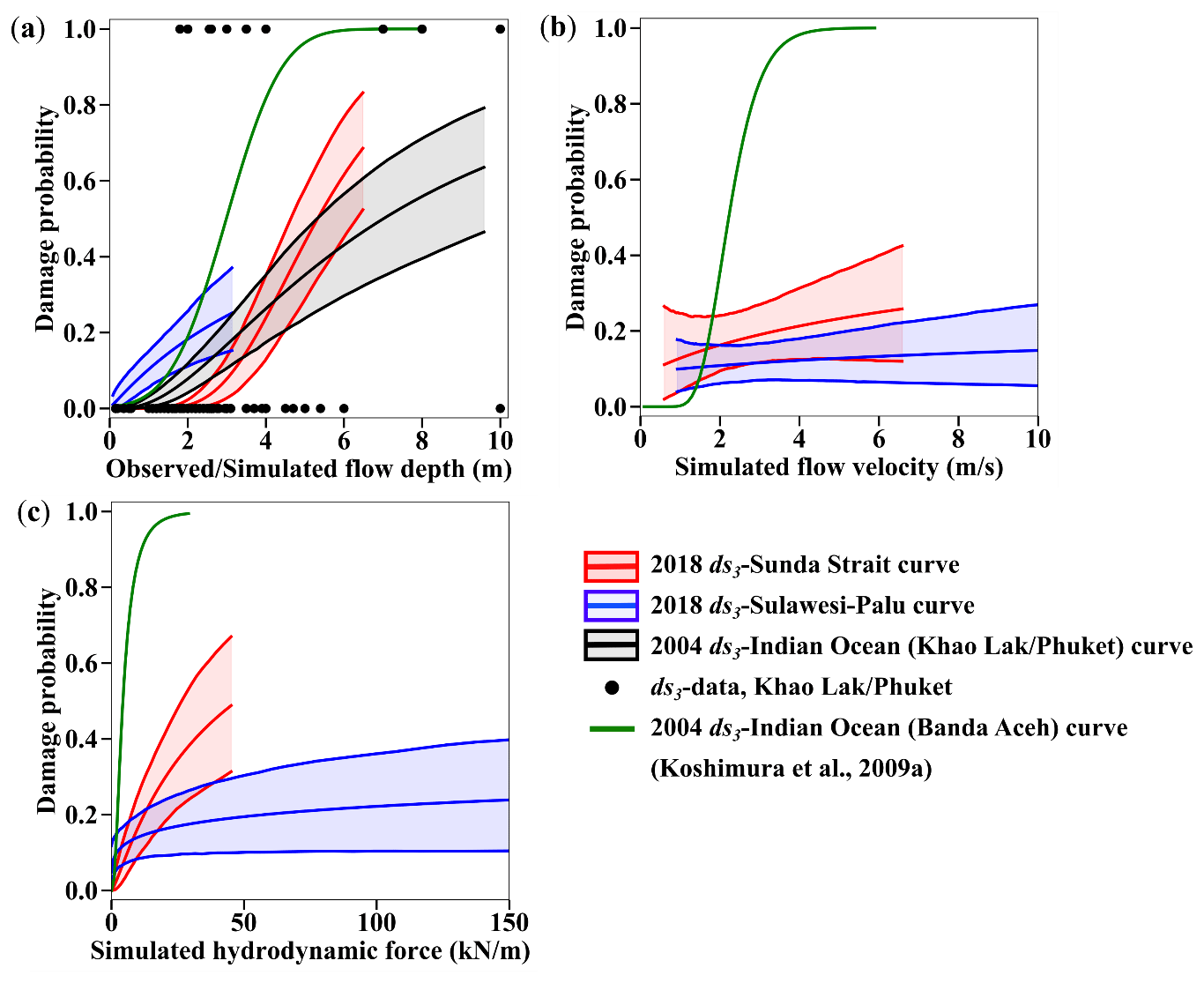
https://nhess.copernicus.org/articles/21/2313/2021/nhess-21-2313-2021-f16

Figure 16Best-estimate fragility curves for the 2018 Sunda Strait tsunami, 2018 Sulawesi–Palu tsunami, and 2004 IOT in Khao Lak–Phuket (Thailand) and Banda Aceh (Indonesia) as functions of (a) the observed and the maximum simulated flow depths, (b) the maximum simulated flow velocity, and (c) the simulated hydrodynamic force. These fragility functions are developed only for completely damaged or washed away buildings with their 90 % confidence intervals.

Download

6 Discussion

6.1 Reliability of the building fragility curves

The reliability of the curves depends mainly on (i) the quality and the quantity of post-tsunami data and (ii) whether the tsunami intensity measures are efficient predictors of damage. With regard to the first factor, DB_Sunda2018, DB_Palu2018, and DB_Thailand2004 include relatively little data (Table 2). For each database, the relatively broad confidence intervals around the best-estimate fragility curves reflect the small sample size. Moreover, the complexity of each studied event also plays a role in how well the selected tsunami intensity measure can represent the tsunami damage. In particular, in DB_Sunda2018 and DB_Thailand2004, only the tsunami load is responsible for the building damage. In contrast, in DB_Palu2018, buildings may have suffered prior damage due to ground shaking and liquefaction (Kijewski-Correa and Robertson, 2018; Sassa and Takagawa, 2019). Nonetheless, we are not able to establish precisely which of the surveyed buildings had suffered prior damage in the database and to what extent. The complexity of the 2018 Sulawesi–Palu event could introduce a bias in the tsunami fragility assessment, and this has also been mentioned for other events such as the 2011 great eastern Japan tsunami (Charvet et al., 2014). This bias could explain why we observed a negative slope for our ds₃-curves based on the observed flow depth combined with very few collapsed buildings, especially for very low intensity levels (Fig. 11). Despite the aforementioned reservations, the adopted statistical tests identified that the flow depth is consistently the best descriptor of the tsunami damage for both the DB_Sunda2018 and DB_Palu2018 data, while the flow velocity is the worst. This finding is in line with similar observations made by Macabuag et al. (2016). De Risi et al. (2017) illustrated well the influence of the DEM resolution and the model sources on the efficiency of the flow velocity as a tsunami intensity measure. In Sunda Strait, the DEM resolution is relatively high (20 m), and it could explain why the flow velocity is not a good descriptor of damage. In Palu City, we perform two-layer numerical modelling using the finest grid size of 1 m. However, the 2018 Palu tsunami is a complex event. The subaerial and submarine landslides may not be the main cause of the tsunami, as shown by Ulrich et al. (2019), and this could have affected the flow velocity data. As the flow velocity of the Sunda Strait and Sulawesi–Palu tsunamis does not provide a good description of the damage, we cannot evaluate the impact of floating debris on Indonesian structures (Song et al., 2017). The hydrodynamic force of these events, computed from the flow velocity and the flow depth, does not provide a good description of the tsunami damage either.

6.2 Impact of the wave period, ground shaking, and liquefaction events on the building damage probability

The curve comparison illustrates well the relationship between the 2004 Indian Ocean, the 2018 Sunda Strait, and the 2018 Sulawesi–Palu tsunamis characteristics, summarized in Table 11, and the structural performance of buildings.

Table 10Damage probabilities of buildings reaching complete damage according to the intensity measures of the 2018 Sunda Strait, 2018 Sulawesi–Palu, and 2004 Indian Ocean (Khao Lak–Phuket and Banda Aceh) tsunamis.

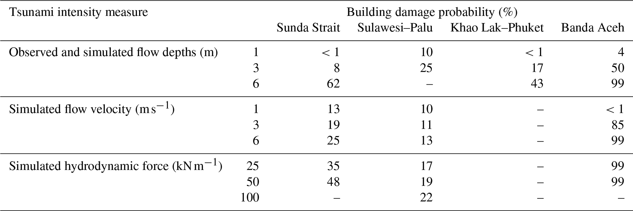
Download Print Version | Download XLSX

Table 11Characteristics of the 2004 Indian Ocean tsunami in Banda Aceh (Indonesia) and Khao Lak–Phuket (Thailand), as well as the 2018 Sulawesi–Palu and 2018 Sunda Strait tsunamis.

+: recorded; –: not recorded.

Download Print Version | Download XLSX

Impact of the wave period

The 2018 Sunda Strait tsunami and the 2004 IOT (Khao Lak–Phuket, Thailand) are characterized by dominant wave periods of about 7 min (Muhari et al., 2019) and 40 min (Karlsson et al., 2009; Puspito and Gunawan, 2005; Tsuji et al., 2006), respectively (Table 11). Damage from ground shaking or liquefaction episodes was not reported, so the tsunami is the main cause of building damage. We compare the Sunda Strait and the Indian Ocean (Khao Lak–Phuket) curves based on the flow depth to investigate the impact of the tsunami wave period on buildings. In Fig. 16a, the curves showed that the short wave period tsunami in the Sunda Strait is less damaging than the 2004 IOT below 5 m flow depth. For instance, for 3 m flow depth, the likelihood of complete damage is around 20 % in Khao Lak–Phuket against only 10 % in the Sunda Strait area (Table 10). On the other hand, above 5 m flow depth, the structures in Khao Lak–Phuket reveal a better performance than the ones in the Sunda Strait area. As few data points are available beyond this value for completely damaged buildings, the Sunda Strait and the Indian Ocean (Khao Lak–Phuket) curve reliability is insufficient. Even though the long wave periods of the IOT seem to increase the likelihood of building damage, the sample size of collapsed buildings beyond 5 m flow depth is too small to validate this assumption.

Impact of ground shaking and liquefaction events

The city of Banda Aceh and the Khao Lak–Phuket area were damaged by the 2004 IOT. Along Banda Aceh shores, the simulated tsunami wave period ranges from 40 to 45 min (Prasetya et al., 2011; Puspito and Gunawan, 2005), and the one simulated in Khao Lak–Phuket is estimated at approximatively 40 min (Karlsson et al., 2009; Puspito and Gunawan, 2005; Tsuji et al., 2006). Although the tsunami wave periods are similar at both locations, the 2004 Indian Ocean earthquake was strongly felt in the city of Banda Aceh, where it lasted about 10 min (Table 11). The earthquake intensity is estimated at VII to VIII on the Modified Mercalli Scale (Ghobarah et al., 2006; Saatcioglu et al., 2006). Despite the ground acceleration not being recorded in the damage zones, seismic failure was distinguished from tsunami damage. For example, buildings with three to five stories were heavily damaged by the ground motion, which was amplified by the soft soil characteristics, compared to low-rise structures. In Fig. 16a, the curves estimate about 50 % and 20 % of building damage probabilities for complete damage in Banda Aceh and Khao Lak–Phuket, respectively, for 3 m flow depth (Table 10). Therefore, the building resilience is higher in Khao Lak–Phuket than in Banda Aceh. It comes from the fact that the Khao Lak–Phuket curve is developed for reinforced concrete buildings, while the ones in Banda Aceh are produced for mixed buildings (Koshimura et al., 2009a). Another reason is that the 2004 Indian Ocean earthquake was not recorded in Khao Lak–Phuket, so the ground motion did not damage the buildings before the tsunami's arrival. Furthermore, the likelihood of complete damage is very high for low inundation depth levels in Banda Aceh. This feature is usually observed for buildings suffering prior damage such as ground shaking and/or liquefactions episodes, as mentioned by Charvet et al. (2014) for the 2011 great eastern Japan event.

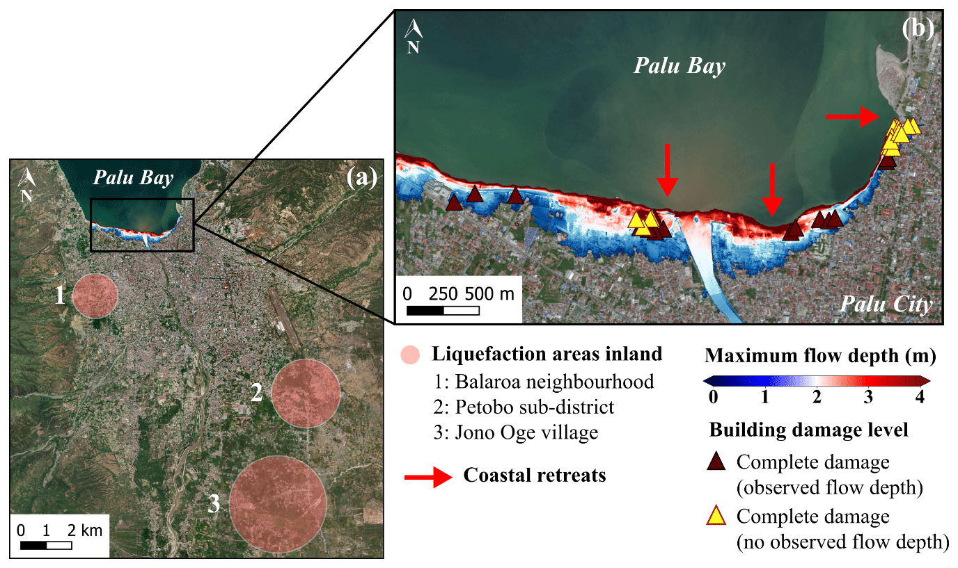
https://nhess.copernicus.org/articles/21/2313/2021/nhess-21-2313-2021-f17

Figure 17(a) Liquefaction areas surveyed inland near Palu City and (b) magnified view of the maximum simulated flow depth of the 2018 Sulawesi–Palu tsunami overlaid on the masonry-type buildings completely damaged (ds₃) and location of the coastal retreats surveyed in the waterfront of Palu City (background ESRI).

The 2018 Sulawesi–Palu event is characterized by short wave periods of about 3.5 min according to Syamsidik et al. (2019), like the 2018 Sunda Strait tsunami (Table 11). However, the curves based on the flow depth are remarkably different (Fig. 16a). For instance, for 3 m flow depth, the likelihood of complete damage is 25 % in Palu against 10 % in Sunda Strait, which means that buildings affected by the Sulawesi–Palu tsunami were more susceptible to complete damage. Most importantly, up to 2 m flow depth, the building damage probability is higher in Palu than in Banda Aceh, affected by ground shaking and then being hit by a long wave period tsunami. As an example, for 1 m flow depth, the building damage probability of complete damage is about 10 % in Palu against less than 5 % in Banda Aceh (Table 10). The main cause of structural damage caused by the Sulawesi–Palu tsunami is still being investigated. Mas et al. (2020) suggested that the tsunami hydrodynamic or debris impact might be the main cause of structural destruction in the waterfront area of Palu Bay. Here, the flow velocity and the hydrodynamic force are not good descriptors of damage, so we cannot support this assumption (Song et al., 2017). On the other hand, Palu City sits on alluvial soil layers from Palu River and is thereby vulnerable to liquefaction disaster (Darma and Sulistyantara, 2020; Goda et al., 2019; Kijewski-Correa and Robertson, 2018). Even though the largest liquefaction areas were recorded outside the inundation zone (Watkinson and Hall, 2019), Sassa and Takagawa (2019) and Kijewski-Correa and Robertson (2018) observed land retreats along the coastal area of Palu City (Fig. 17a and b). Most of the masonry-type buildings completely damaged are very close to these coastal retreats. Some of them were washed away by the tsunami. Therefore, these buildings do not have flow depth values and could not be used for the tsunami fragility assessment (Fig. 17b). Furthermore, in Palu, the earthquake intensity is estimated at VII to VIII on the Modified Mercalli Scale, but ground shaking was not the main cause of structural destruction (Kijewski-Correa and Robertson, 2018; Supendi et al., 2019). The likelihood of complete damage is also relatively high for low flow depth levels, so ground motion could have triggered liquefaction events and enhanced the building susceptibility to tsunami damage in the waterfront of Palu City. This assumption cannot be verified through satellite images; it needs direct and close observations, which might be erased by the tsunami.

7 Conclusions

According to the GEM guidelines, building fragility curves of the 2018 Sunda Strait, 2018 Sulawesi–Palu, and 2004 Indian Ocean (Khao Lak–Phuket, Thailand) tsunamis are empirically developed from post-tsunami databases respectively called DB_Sunda2018, DB_Palu2018, and DB_Thailand2004. To improve our understanding of the structural damage caused by the Sunda Strait and Sulawesi–Palu tsunamis, we reproduce their tsunami intensity measures (i.e., flow depth, flow velocity, and hydrodynamic force) with the TUNAMI two-layer model for the first time. The flow depth is constantly the best descriptor of tsunami damage for each event. The building fragility curves for complete damage reveal the following. (i) The buildings affected by the Sunda Strait tsunami sustained less damage than the ones in Khao Lak–Phuket (IOT). For example, for 3 m flow depth, the building damage probability is around 20 % in Khao Lak–Phuket against 10 % in the Sunda Strait area hit by a short wave period tsunami (landslide source). Considering that the tsunami was the main cause of structural damage (i.e., damage related to ground shaking and/or liquefaction was not recorded), the longer wave period of the 2004 IOT may have increased the likelihood of complete damage, and (ii) the building resilience is weaker in Banda Aceh than in Khao Lak–Phuket. For 3 m flow depth, the likelihood of complete damage is about 50 % in Banda Aceh and 20 % in Khao Lak–Phuket. Although both locations were hit by the 2004 IOT, Banda Aceh was strongly affected by ground shaking before the tsunami's arrival, and (iii) the buildings affected by the Sulawesi–Palu tsunami were more susceptible to be completely damaged than the ones affected by the IOT in Banda Aceh (i.e., ≤2 m). As an example, for 1 m flow depth, the building damage probability of complete damage is about 10 % in Palu and 5 % in Banda Aceh. The Sulawesi–Palu tsunami is a complex event as it may not be the only cause of structural destruction. The 2018 Sulawesi earthquake caused minor damage to buildings and most importantly could have triggered liquefaction events in the waterfront of Palu City where coastal retreats have been observed, increasing the susceptibility of buildings to tsunami damage.

Appendix A: Two-layer modelling of a subaerial and submarine landslide

https://nhess.copernicus.org/articles/21/2313/2021/nhess-21-2313-2021-f18

Figure A1Two-layer modelling of a subaerial and submarine landslide (from the original sketch of Pakoksung et al., 2019): (a) pre-failure, (b) generation of negative and positive waves due to the landslide, and (c) landslide in progress and wave propagation.

Download

Appendix B: The 2018 Sunda Strait tsunami generation, propagation, and inundation modelling

https://nhess.copernicus.org/articles/21/2313/2021/nhess-21-2313-2021-f19

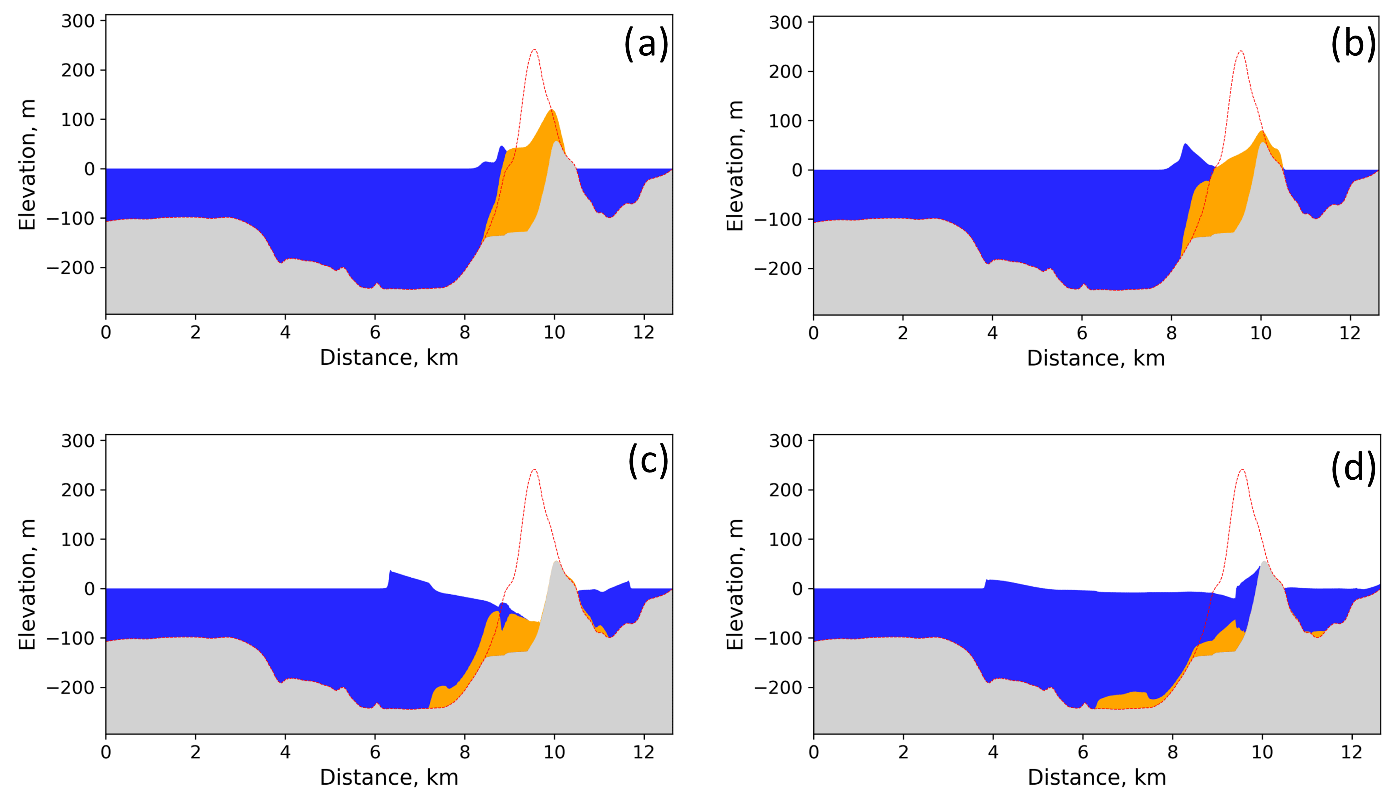
Figure B1Temporal evolution of the 2018 Sunda Strait tsunami wave (a) 10, (b) 20, (c) 60, and (d) 120 s after the volcano flank collapse. The red line is the topography and bathymetry before the landslide (Pakoksung et al., 2020).

Download

https://nhess.copernicus.org/articles/21/2313/2021/nhess-21-2313-2021-f20

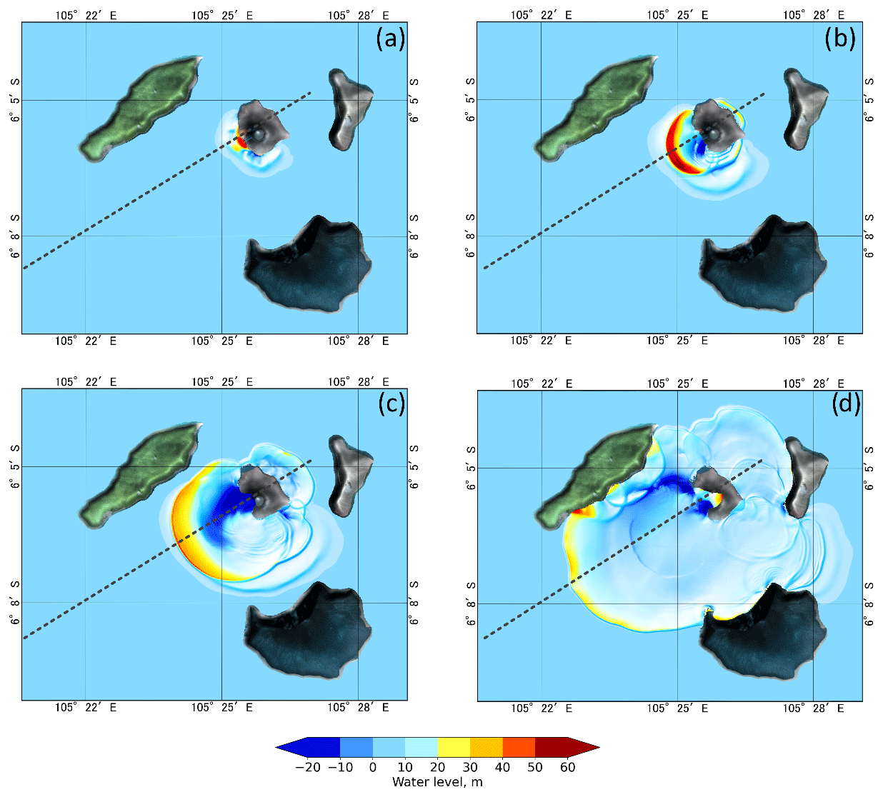
Figure B2Temporal evolution of the 2018 Sunda Strait tsunami wave (a) 10, (b) 20, (c) 60, and (d) 120 s after the volcano flank collapse (Pakoksung et al., 2020).

Download

https://nhess.copernicus.org/articles/21/2313/2021/nhess-21-2313-2021-f21

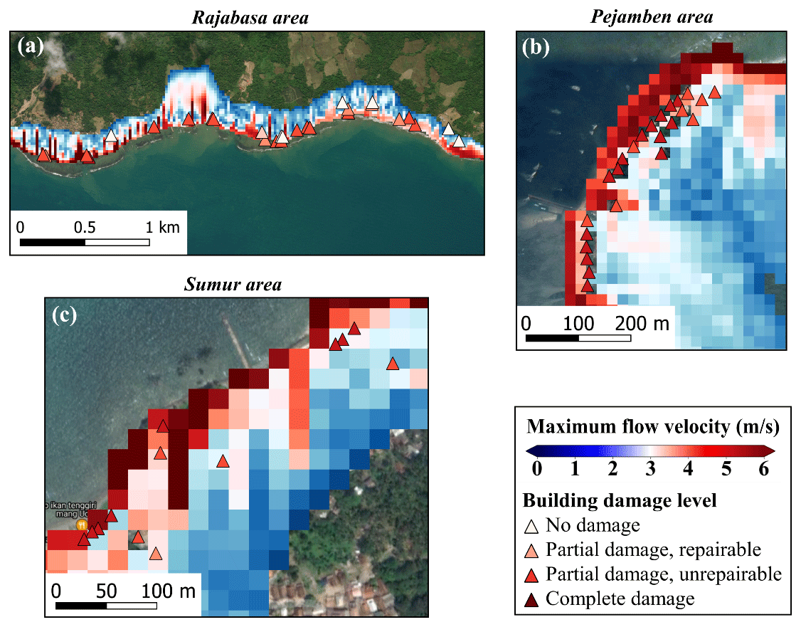
Figure B3(a–c) Magnified views of the maximum simulated flow velocity of the 2018 Sunda Strait tsunami overlaid on the damaged building data in the Rajabasa, Pejamben, and Sumur areas (background ESRI and © Google Maps).

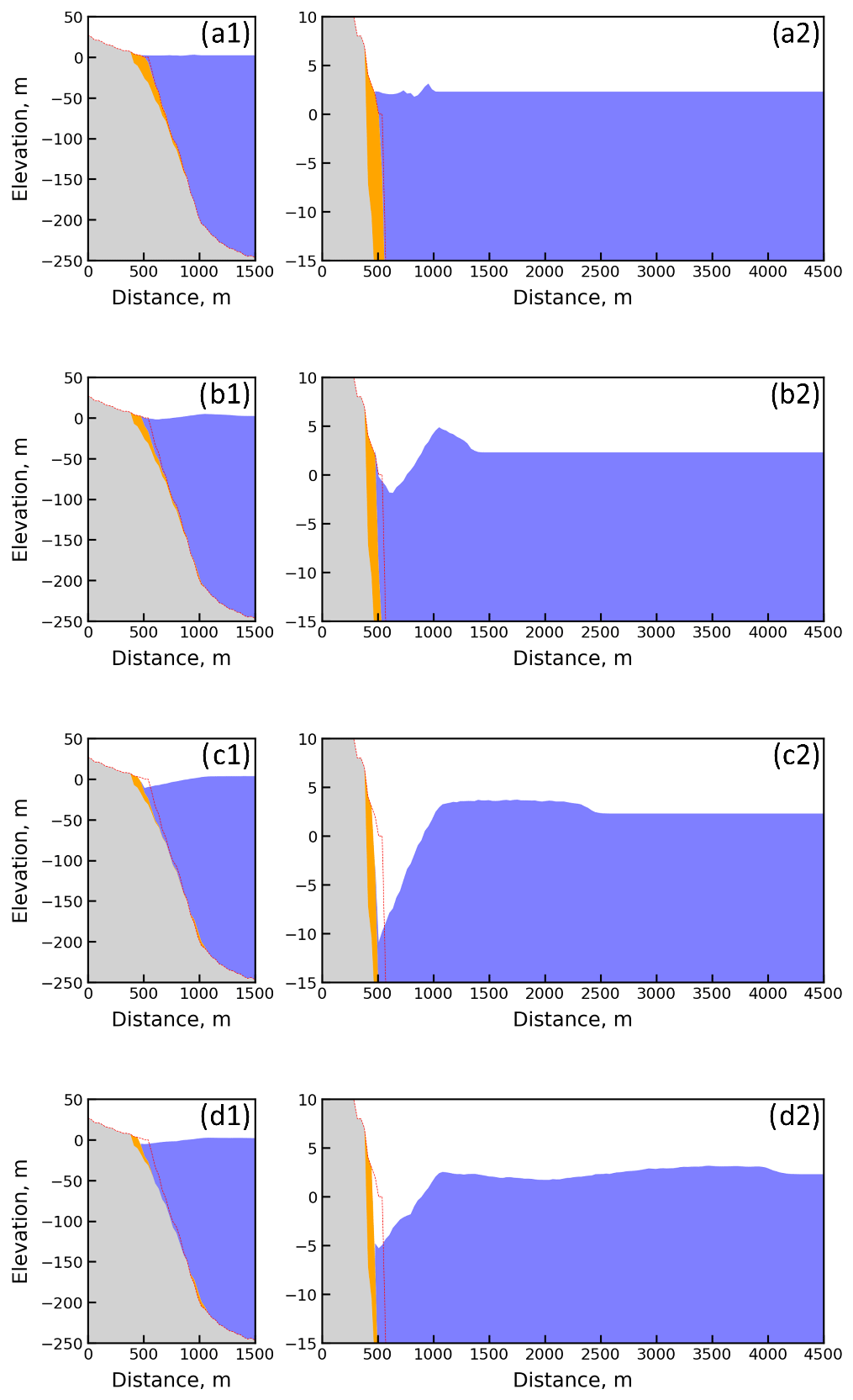
Appendix C: The 2018 Sulawesi–Palu tsunami generation, propagation, and inundation modelling

https://nhess.copernicus.org/articles/21/2313/2021/nhess-21-2313-2021-f22

Figure C1Temporal evolution of the 2018 Sulawesi–Palu tsunami wave (a) 2, (b) 10, (c) 30, and (d) 60 s after the S8 landslide. The red line is the topography and bathymetry before S8 landslide (Pakoksung et al., 2019).

Download

https://nhess.copernicus.org/articles/21/2313/2021/nhess-21-2313-2021-f23

Figure C2Temporal evolution of the 2018 Sulawesi–Palu tsunami wave (a) 2, (b) 10, (c) 30, and (d) 60 s after the S8 landslide (Pakoksung et al., 2019).

Download

https://nhess.copernicus.org/articles/21/2313/2021/nhess-21-2313-2021-f24

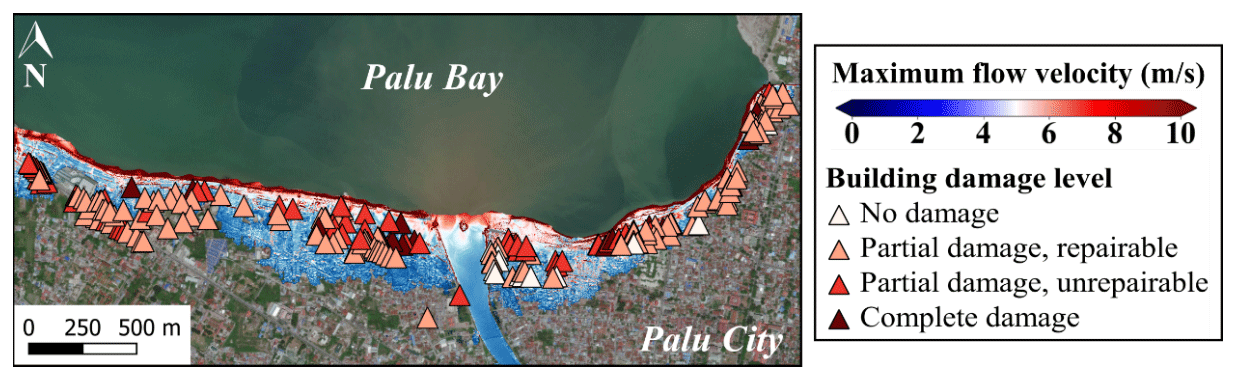
Figure C3Sulawesi–Palu final tsunami inundation model with the maximum simulated flow velocity overlaid on the damaged building data (background ESRI).

Appendix D: Statistical model selection: comparison of AIC values for logit and cloglog link functions (DB_Sunda2018)

Table D1AIC values for the three models assuming logit and cloglog link functions fitted to the observed and simulated tsunami intensity measures of DB_Sunda2018.

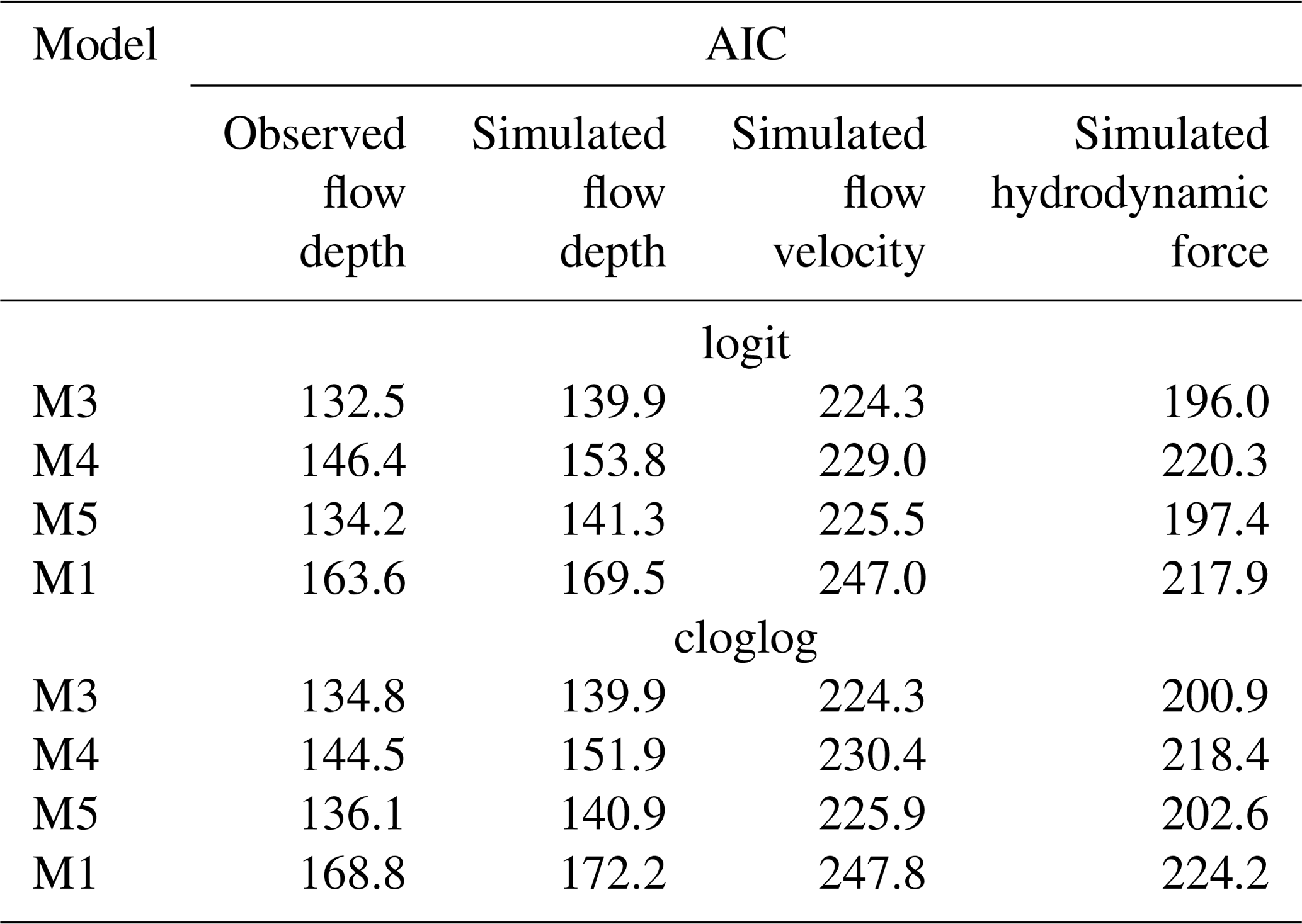
Download Print Version | Download XLSX

Appendix E: Regression coefficients for the building fragility curves of the 2018 Sunda Strait, 2018 Sulawesi–Palu, and 2004 Indian Ocean (Khao Lak–Phuket) tsunamis

Table E1Regression coefficients for the 2018 Sunda Strait tsunami fragility curves based on DB_Sunda2018.

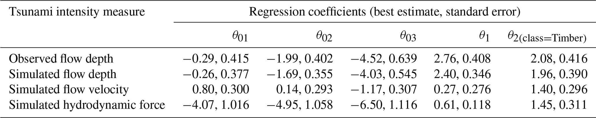
Download Print Version | Download XLSX

Table E2Regression coefficients for the 2018 Sulawesi–Palu tsunami fragility curves based on DB_Palu2018.

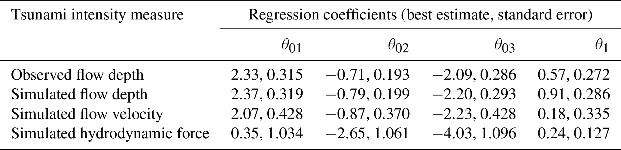
Download Print Version | Download XLSX

Table E3Regression coefficients for the 2004 IOT in Khao Lak–Phuket (Thailand) based on DB_Thailand2004.

Download Print Version | Download XLSX

Code and data availability

Post-tsunami field survey data are available from references cited in the text. The bathymetric and topographic data for the Sunda Strait area were provided by BATNAS and DEMNAS, Indonesia, respectively (http://tides.big.go.id/DEMNAS/index.html, last access: 1 February 2020) (DEMNAS, 2020). The Geospatial Information Agency (BIG), Indonesia, provided the bathymetric and topographic data for Palu Bay. The tidal gauge records were supplied by the Coastal Disaster Mitigation Division, Ministry of Marine Affairs and Fisheries, Jakarta, Indonesia. Spatial data in this study are depicted through QGIS software.

Author contributions

FI, AS, KP, EL, II, and FB designed and coordinated this research. AS, KP, and EL performed the tsunami simulations and participated in the calibration of the inundation models in Palu Bay and in Sunda Strait. SS and RP contributed to the tsunami data collection in the Sunda Strait and Palu areas, respectively. II developed the fragility functions through advanced statistical analysis. All authors contributed to the drafting of the manuscript.

Competing interests

The authors declare that they have no conflict of interest.

Acknowledgements

We greatly acknowledge the three reviewers for their constructive comments and recommendations that helped to improve the quality of this manuscript. This research was funded and supported by the Japan Society for the Promotion of Science (JSPS) Grant-in-Aid for Young Scientists, the JSPS-NRCT Bilateral Research grant, the World Class Professor (WCP) programme 2018–2020 promoted by the Ministry of Education and Culture of the Republic of Indonesia, the Pacific Consultants Co., Ltd., the Willis Research Network (WRN), the Tokio Marine & Nichido Fire Insurance Co., Ltd., the National Institute of Water and Atmospheric Research (Project: CARH2106), UKRI GCRF Urban Disaster Risk Hub, and GLADYS.

Disclaimer

Publisher's note: Copernicus Publications remains neutral with regard to jurisdictional claims in published maps and institutional affiliations.

Financial support

This research has been supported by the Japan Society for the Promotion of Science (Grant-in-Aid for Young Scientists (B)), the National Research Council of Thailand (Bilateral Research grant, fiscal year 2017–2018), the Kementerian Riset Teknologi Dan Pendidikan Tinggi Republik Indonesia (World Class Professor, WCP, programme 2018–2020), the Université de Montpellier (grant GLADYS), the Global Challenges Research Fund (grant no. Urban Disaster Risk Hub NE/S009000/1), the National Institute of Water and Atmospheric Research (project: CARH2106), Pacific Consultants Co., Ltd., Willis Research Network (WRN), and Tokio Marine & Nichido Fire Insurance Co., Ltd.

Review statement

This paper was edited by Maria Ana Baptista and reviewed by three anonymous referees.

References

Aburaya, T. and Imamura, F.: The proposal of a tsunami run-up simulation using combined equivalent roughness, Annual Journal of Coastal Engineering, Japan Society of Civil Engineers, 49, 276–280, 2002.

Aida, I.: Reliability of a tsunami source model derived from fault parameters, J. Phys. Earth, 26, 57–73, https://doi.org/10.4294/jpe1952.26.57, 1978.

Akaike, H.: A new look at the statistical model identification, IEEE T. Automat. Contr., 19, 716–723, https://doi.org/10.1109/TAC.1974.1100705, 1974.

Ammon, C. J., Ji, C., Thio, H.-K., Robinson, D., Ni, S., Hjorleifsdottir, V., Kanamori, H., Lay, T., Das, S., and Helmberger, D.: Rupture process of the 2004 Sumatra-Andaman earthquake, Science, 308, 1133–1139, https://doi.org/10.1126/science.1112260, 2005.

Arikawa, T., Muhari, A., Okumura, Y., Dohi, Y., Afriyanto, B., Sujatmiko, K. A., and Imamura, F.: Coastal subsidence induced several tsunamis during the 2018 Sulawesi earthquake, Journal of Disaster Research, 13, 1–3, https://doi.org/10.20965/jdr.2018.sc20181204, 2018.

Asian Disaster Preparedness Center: The economic impact of the 26 December 2004 earthquake and Indian Ocean tsunami in Thailand, available at: https://reliefweb.int/report/thailand/economic-impact-26-december-2004-earthquake-and-indian-ocean-tsunami-thailand (last access: 15 February 2020), 2007.

Association of Southeast Asian Nations (ASEAN)-Coordinating Centre for Humanitarian Assistance on disaster: Situation update No. 12 M 7.4 earthquake and tsunami Sulawesi, Indonesia, available at: https://reliefweb.int/sites/reliefweb.int/files/resources/AHA-Situation_Update-no12-Sulawesi-EQ-rev.pdf (last access: 20 February 2020), 2018.

Attary, N., Van de Lindt, J. W., Unnikrishnan, V. U., Barbosa, A. R., and Cox, D. T.: Methodology for development of physics-based tsunami fragilities, J. Struct. Eng., 143, 04016223, https://doi.org/10.1061/(ASCE)ST.1943-541X.0001715, 2017.

Carvajal, M., Araya-Cornejo, C., Sepúlveda, I., Melnick, D., and Haase, J. S.: Nearly instantaneous tsunamis following the Mw 7.5 2018 Palu earthquake, Geophys. Res. Lett., 46, 5117–5126, https://doi.org/10.1029/2019GL082578, 2019.

Chakrabarti, S.: Handbook of Offshore Engineering (2-volume set), Elsevier, Plainfield, Illinois, USA, 2005.

Charvet, I., Ioannou, I., Rossetto, T., Suppasri, A., and Imamura, F.: Empirical fragility assessment of buildings affected by the 2011 Great East Japan tsunami using improved statistical models, Nat. Hazards, 73, 951–973, https://doi.org/10.1007/s11069-014-1118-3, 2014.

Darma, Y. and Sulistyantara, B.: Analysis of landscape impact on post-earthquake, tsunami, and liquefaction disasters in Palu City, Central Sulawesi, in: IOP Conference Series: Earth and Environmental Science, vol. 501, p. 012003, IOP Publishing, Bogor, Indonesia, 2020.

Day, S. J.: Volcanic tsunamis, in: The Encyclopedia of Volcanoes, Sigurdsson, H., Houghton, B., McNutt, S., Rymer, H., and Stix, J. (Eds.), 993–1009, Elsevier, Amsterdam, 2015.

DEMNAS: Seamless Digital Elevation Model (DEM) dan Batimetri Nasional, [data], available at: http://tides.big.go.id/DEMNAS/index.html, last access: 1 February 2020.

De Risi, R., Goda, K., Yasuda, T., and Mori, N.: Is flow velocity important in tsunami empirical fragility modeling?, Earth-Sci. Rev., 166, 64–82, https://doi.org/10.1016/j.earscirev.2016.12.015, 2017.

Dogan, G. G., Annunziato, A., Hidayat, R., Husrin, S., Prasetya, G., Kongko, W., Zaytsev, A., Pelinovsky, E., Imamura, F., and Yalciner, A. C.: Numerical simulations of December 22, 2018 Anak Krakatau tsunami and examination of possible submarine landslide scenarios, Pure Appl. Geophys., 1–20, https://doi.org/10.1007/s00024-020-02641-7, 2021.

Federal Emergency Management Agency (FEMA): Coastal construction manual, FEMA 55, USA, 296 pp., 2003.

Foytong, P. and Ruangrassamee, A.: Fragility curves of reinforced-concrete buildings damaged by a tsunami for tsunami risk analysis, in: The Twentieth KKCNN Symposium on Civil Engineering, October 2007, Jeju, Korea, 4–5, 2007.

Frederik, M. C. G., Udrekh, Adhitama, R., Hananto, N. D., Asrafil, Sahabuddin, S., Irfan, M., Moefti, O., Putra, D. B., and Riyalda, B. F.: First results of a bathymetric survey of Palu Bay, Central Sulawesi, Indonesia following the tsunamigenic earthquake of 28 September 2018, Pure Appl. Geophys., 176, 3277–3290, https://doi.org/10.1007/s00024-019-02280-7, 2019.

Ghobarah, A., Saatcioglu, M., and Nistor, I.: The impact of the 26 December 2004 earthquake and tsunami on structures and infrastructure, Eng. Struct., 28, 312–326, https://doi.org/10.1016/j.engstruct.2005.09.028, 2006.

Goda, K., Mori, N., Yasuda, T., Prasetyo, A., Muhammad, A., and Tsujio, D.: Cascading geological hazards and risks of the 2018 Sulawesi Indonesia earthquake and sensitivity analysis of tsunami inundation simulations, Front. Earth Sci., 7, 261, https://doi.org/10.3389/feart.2019.00261, 2019.

Gokon, H., Koshimura, S., Matsuoka, M., and Namegaya, Y.: Developing tsunami fragility curves due to the 2009 tsunami disaster in American Samoa, Journal of Japan Society of Civil Engineers, Ser. B2 (Coastal Engineering), 67, 1321–1325, https://doi.org/10.2208/kaigan.67.I_1321, 2011.

Grezio, A., Babeyko, A., Baptista, M. A., Behrens, J., Costa, A., Davies, G., Geist, E. L., Glimsdal, S., González, F. I., Griffin, J., Harbitz, C. B., LeVeque, R. J., Lorito, S., Løvholt, F., Omira, R., Mueller, C., Paris, R., Parsons, T., Polet, J., Power, W., Selva, J., Sørensen, M. B., and Thio, H. K.: Probabilistic tsunami hazard analysis: multiple sources and global applications, Rev. Geophys., 55, 1158–1198, https://doi.org/10.1002/2017RG000579, 2017.

Grilli, S. T., Tappin, D. R., Carey, S., Watt, S. F. L., Ward, S. N., Grilli, A. R., Engwell, S. L., Zhang, C., Kirby, J. T., Schambach, L., and Muin, M.: Modelling of the tsunami from the December 22, 2018 lateral collapse of Anak Krakatau volcano in the Sunda Straits, Indonesia, Sci. Rep.-UK, 9, 1–13, https://doi.org/10.1038/s41598-019-48327-6, 2019.

Gusman, A. R., Supendi, P., Nugraha, A. D., Power, W., Latief, H., Sunendar, H., Widiyantoro, S., Wiyono, S. H., Hakim, A., and Muhari, A.: Source model for the tsunami inside palu bay following the 2018 palu earthquake, Indonesia, Geophys. Res. Lett., 46, 8721–8730, https://doi.org/10.1029/2019gl082717, 2019.

Heidarzadeh, M., Muhari, A., and Wijanarto, A. B.: Insights on the source of the 28 September 2018 Sulawesi tsunami, Indonesia based on spectral analyses and numerical simulations, Pure Appl. Geophys., 176, 25–43, https://doi.org/10.1007/s00024-018-2065-9, 2019.

Heidarzadeh, M., Ishibe, T., Sandanbata, O., Muhari, A., and Wijanarto, A. B.: Numerical modeling of the subaerial landslide source of the 22 December 2018 Anak Krakatoa volcanic tsunami, Indonesia, Ocean Eng., 195, 106733, https://doi.org/10.1016/j.oceaneng.2019.106733, 2020.

Imamura, F. and Imteaz, M. A.: Long waves in two layers: governing equations and numerical model, Science of Tsunami Hazards, 13, 3–24, 1995.

Japan Society of Civil Engineers (JSCE): Tsunami assessment method for nuclear power plants in Japan, Japan Society of Civil Engineers Tokyo, available at: https://www.jsce.or.jp/committee/ceofnp/Tsunami/eng/JSCE_Tsunami_060519.pdf (last access: 28 January 2020), 2002.

Karlsson, J. M., Skelton, A., Sandén, M., Ioualalen, M., Kaewbanjak, N., Pophet, N., Asavanant, J., and Von Matern, A.: Reconstructions of the coastal impact of the 2004 Indian Ocean tsunami in the Khao Lak area, Thailand, J. Geophys. Res.-Oceans, 114, C10023, https://doi.org/10.1029/2009JC005516, 2009.

Kijewski-Correa, T. and Robertson, I.: StEER: structural extreme event reconnaissance network: Palu earthquake and tsunami, Sulawesi, Indonesia field assessment Team 1 (FAT-1), early access reconnaissance report (EARR), 2018.

Koshimura, S., Oie, T., Yanagisawa, H., and Imamura, F.: Developing fragility functions for tsunami damage estimation using numerical model and post-tsunami data from Banda Aceh, Indonesia, Coast. Eng. J., 51, 243–273, https://doi.org/10.1142/S0578563409002004, 2009a.

Koshimura, S., Namegaya, Y., and Yanagisawa, H.: Tsunami fragility – A new measure to identify tsunami damage, Journal of Disaster Research, 4, 479–488, https://doi.org/10.20965/jdr.2009.p0479, 2009b.

Kotani, M.: Tsunami run-up simulation and damage estimation using GIS, Pacific Coast Engineering, Japan Society of Civil Engineers (JSCE), 45, 356–360, 1998.

Krüger, F. and Ohrnberger, M.: Spatio-temporal source characteristics of the 26 December 2004 Sumatra earthquake as imaged by teleseismic broadband arrays, Geophys. Res. Lett., 32, L24312, https://doi.org/10.1029/2005GL023939, 2005.

Lauterjung, J., Münch, U., and Rudloff, A.: The challenge of installing a tsunami early warning system in the vicinity of the Sunda Arc, Indonesia, Nat. Hazards Earth Syst. Sci., 10, 641–646, https://doi.org/10.5194/nhess-10-641-2010, 2010.

Lavigne, F., Paris, R., Grancher, D., Wassmer, P., Brunstein, D., Vautier, F., Leone, F., Flohic, F., De Coster, B., Gunawan, T., Gomez, C., Setiawan, A., Cahyadi, R., and Fachrizal: Reconstruction of tsunami inland propagation on December 26, 2004 in Banda Aceh, Indonesia, through field investigations, Pure Appl. Geophys., 166, 259–281, https://doi.org/10.1007/s00024-008-0431-8, 2009.

Lay, T., Kanamori, H., Ammon, C. J., Nettles, M., Ward, S. N., Aster, R. C., Beck, S. L., Bilek, S. L., Brudzinski, M. R., and Butler, R.: The great Sumatra-Andaman earthquake of 26 December 2004, Science, 308, 1127–1133, https://doi.org/10.1126/science.1112250, 2005.

Løvholt, F., Bungum, H., Harbitz, C. B., Glimsdal, S., Lindholm, C. D., and Pedersen, G.: Earthquake related tsunami hazard along the western coast of Thailand, Nat. Hazards Earth Syst. Sci., 6, 979–997, https://doi.org/10.5194/nhess-6-979-2006, 2006.

Macabuag, J., Rossetto, T., and Lloyd, T.: Sensitivity analyses of a framed structure under several tsunami design-guidance loading regimes, in: 2nd European Conference on Earthquake Engineering and Seismology, Istanbul, Turkey, available at: http://www.eaee.org/Media/Default/2ECCES/2ecces_eaee/295.pdf (last access: 3 March 020), 2014.

Macabuag, J., Rossetto, T., Ioannou, I., Suppasri, A., Sugawara, D., Adriano, B., Imamura, F., Eames, I., and Koshimura, S.: A proposed methodology for deriving tsunami fragility functions for buildings using optimum intensity measures, Nat. Hazards, 84, 1257–1285, https://doi.org/10.1007/s11069-016-2485-8, 2016.

Macías, J., Vázquez, J. T., Fernández-Salas, L. M., González-Vida, J. M., Bárcenas, P., Castro, M. J., Díaz-del-Río, V., and Alonso, B.: The Al-Borani submarine landslide and associated tsunami. A modelling approach, Mar. Geol., 361, 79–95, https://doi.org/10.1016/j.margeo.2014.12.006, 2015.

Marfai, M. A., King, L., Singh, L. P., Mardiatno, D., Sartohadi, J., Hadmoko, D. S., and Dewi, A.: Natural hazards in Central Java Province, Indonesia: an overview, Environ. Geol., 56, 335–351, https://doi.org/10.1007/s00254-007-1169-9, 2008.

Mas, E., Koshimura, S., Suppasri, A., Matsuoka, M., Matsuyama, M., Yoshii, T., Jimenez, C., Yamazaki, F., and Imamura, F.: Developing Tsunami fragility curves using remote sensing and survey data of the 2010 Chilean Tsunami in Dichato, Nat. Hazards Earth Syst. Sci., 12, 2689–2697, https://doi.org/10.5194/nhess-12-2689-2012, 2012.

Mas, E., Paulik, R., Pakoksung, K., Adriano, B., Moya, L., Suppasri, A., Muhari, A., Khomarudin, R., Yokoya, N., Matsuoka, M., and Koshimura, S.: Characteristics of tsunami fragility functions developed using different sources of damage data from the 2018 Sulawesi earthquake and tsunami, Pure Appl. Geophys., 177, 2437–2455, https://doi.org/10.1007/s00024-020-02501-4, 2020.

McCloskey, J., Antonioli, A., Piatanesi, A., Sieh, K., Steacy, S., Nalbant, S., Cocco, M., Giunchi, C., Huang, J., and Dunlop, P.: Tsunami threat in the Indian Ocean from a future megathrust earthquake west of Sumatra, Earth Planet. Sc. Lett., 265, 61–81, https://doi.org/10.1016/j.epsl.2007.09.034, 2008.

Muhari, A., Imamura, F., Arikawa, T., Hakim, A. R., and Afriyanto, B.: Solving the puzzle of the September 2018 Palu, Indonesia, tsunami mystery: clues from the tsunami waveform and the initial field survey data, Journal of Disaster Research, 13(Scientific Communication), sc20181108, https://doi.org/10.20965/jdr.2018.sc20181108, 2018.

Muhari, A., Heidarzadeh, M., Susmoro, H., Nugroho, H. D., Kriswati, E., Supartoyo, Wijanarto, A. B., Imamura, F., and Arikawa, T.: The December 2018 Anak Krakatau Volcano tsunami as inferred from post-tsunami field Surveys and Spectral Analysis, Pure Appl. Geophys., 176, 5219–5233, https://doi.org/10.1007/s00024-019-02358-2, 2019.

Murao, O. and Nakazato, H.: Development of fragility curves for buildings based on damage survey data in Sri Lanka after the 2004 Indian Ocean tsunami, Journal of Structural and Construction Engineering, 75, 1021–1027, https://doi.org/10.3130/aijs.75.1021, 2010.

Nalbant, S. S., Steacy, S., Sieh, K., Natawidjaja, D., and McCloskey, J.: Earthquake risk on the Sunda trench, Nature, 435, 756–757, https://doi.org/10.1038/nature435756a, 2005.

National Agency for Disaster Management (BNPB): The Sunda Strait tsunami, available at: https://reliefweb.int/report/indonesia/indonesia-sunda-strait-tsunami-dg-echo-bnpb-ocha-ifrc-media-echo-daily-flash-23 (last access: 5 March 2020), 2018.

Omira, R. and Ramalho, I.: Evidence-calibrated numerical model of December 22, 2018, Anak Krakatau flank collapse and tsunami, Pure Appl. Geophys., 177, 3059–3071, https://doi.org/10.1007/s00024-020-02532-x, 2020.

Omira, R., Dogan, G. G., Hidayat, R., Husrin, S., Prasetya, G., Annunziato, A., Proietti, C., Probst, P., Paparo, M. A., Wronna, M., Zaytsev, A., Pronin, P., Giniyatullin, A., Putra, P. S., Hartanto, D., Ginanjar, G., Kongko, W., Pelinovsky, E., and Yalciner, A. C.: The September 28th, 2018, tsunami in Palu-Sulawesi, Indonesia: a post-event field survey, Pure Appl. Geophys., 176, 1379–1395, https://doi.org/10.1007/s00024-019-02145-z, 2019.

Otake, T., Chua, C. T., Suppasri, A., and Imamura, F.: Justification of possible casualty-reduction countermeasures based on global tsunami hazard assessment for tsunami-prone regions over the past 400 years, Journal of Disaster Research, 15, 490–502, https://doi.org/10.20965/jdr.2020.p0490, 2020.

Pakoksung, K., Suppasri, A., and Imamura, F.: Systematic evaluation of different infrastructure systems for tsunami defense in Sendai City, Geosciences, 8, 173, https://doi.org/10.3390/geosciences8050173, 2018.

Pakoksung, K., Suppasri, A., Imamura, F., Athanasius, C., Omang, A., and Muhari, A.: Simulation of the submarine landslide tsunami on 28 September 2018 in Palu Bay, Sulawesi Island, Indonesia, using a two-layer model, Pure Appl. Geophys., 176, 3323–3350, https://doi.org/10.1007/s00024-019-02235-y, 2019.

Pakoksung, K., Suppasri, A., Muhari, A., Syamsidik, and Imamura, F.: Global optimization of a numerical two-layer model using observed data: a case study of the 2018 Sunda Strait tsunami, Geoscience Letters, 7, 1–20, https://doi.org/10.1186/s40562-020-00165-5, 2020.

Paris, A., Heinrich, P., Paris, R., and Abadie, S.: The December 22, 2018 Anak Krakatau, Indonesia, landslide and tsunami: preliminary modeling results, Pure Appl. Geophys., 177, 571–590, https://doi.org/10.1007/s00024-019-02394-y, 2020.

Paulik, R., Gusman, A., Williams, J. H., Pratama, G. M., Lin, S., Prawirabhakti, A., Sulendra, K., Zachari, M. Y., Fortuna, Z. E. D., Layuk, N. B. P., and Suwarni, N. W. I.: Tsunami hazard and built environment damage observations from Palu City after the September 28 2018 Sulawesi earthquake and tsunami, Pure Appl. Geophys., 176, 3305–3321, https://doi.org/10.1007/s00024-019-02254-9, 2019.

Prasetya, G., Borrero, J., de Lange, W., Black, K., and Healy, T.: Modeling of inundation dynamics on Banda Aceh, Indonesia during the great Sumatra tsunamis December 26, 2004, Nat. Hazards, 58, 1029–1055, https://doi.org/10.1007/s11069-010-9710-7, 2011.

Puspito, N. T. and Gunawan, I.: Tsunami sources in the sumatra region, Indonesia and simulation of the 26 December 2004 Aceh tsunami, ISET Journal of Earthquake Technology, 42, 4, 2005.

Rastogi, B.: A historical account of the earthquakes and tsunamis in the Indian Ocean, in: The Indian Ocean Tsunami, 3–18, Taylor & Francis, London, 2007.

Reese, S., Cousins, W. J., Power, W. L., Palmer, N. G., Tejakusuma, I. G., and Nugrahadi, S.: Tsunami vulnerability of buildings and people in South Java – field observations after the July 2006 Java tsunami, Nat. Hazards Earth Syst. Sci., 7, 573–589, https://doi.org/10.5194/nhess-7-573-2007, 2007.

Rossetto, T., Peiris, N., Pomonis, A., Wilkinson, S. M., Del Re, D., Koo, R., and Gallocher, S.: The Indian Ocean tsunami of December 26, 2004: observations in Sri Lanka and Thailand, Nat. Hazards, 42, 105–124, https://doi.org/10.1007/s11069-006-9064-3, 2007.

Rossetto, T., Ioannou, I., and Grant, D. N.: Existing empirical fragility and vulnerability relationships: compendium and guide for selection, GEM Fundation, Pavia, 2013.

Rossetto, T., Ioannou, I., Grant, D., and Maqsood, T.: Guidelines for the empirical vulnerability assessment, available at: https://discovery.ucl.ac.uk/id/eprint/1449624/1/Rossetto_ULN-MOD-Empirical-vulnerability-201411-v01.pdf (last access: 16 February 2020), 2014.

Ruangrassamee, A., Yanagisawa, H., Foytong, P., Lukkunaprasit, P., Koshimura, S., and Imamura, F.: Investigation of tsunami-induced damage and fragility of buildings in Thailand after the December 2004 Indian Ocean tsunami, Earthq. Spectra, 22, 377–401, https://doi.org/10.1193/1.2208088, 2006.

Saatcioglu, M., Ghobarah, A., and Nistor, I.: Performance of structures in Indonesia during the December 2004 Great Sumatra earthquake and Indian Ocean tsunami, Earthq. Spectra, 22, 295–319, https://doi.org/10.1193/1.2209171, 2006.

Sassa, S. and Takagawa, T.: Liquefied gravity flow-induced tsunami: first evidence and comparison from the 2018 Indonesia Sulawesi earthquake and tsunami disasters, Landslides, 16, 195–200, https://doi.org/10.1007/s10346-018-1114-x, 2019.

Socquet, A., Hollingsworth, J., Pathier, E., and Bouchon, M.: Evidence of supershear during the 2018 magnitude 7.5 Palu earthquake from space geodesy, Nat. Geosci., 12, 192–199, https://doi.org/10.1038/s41561-018-0296-0, 2019.

Song, J., De Risi, R., and Goda, K.: Influence of flow velocity on tsunami loss estimation, Geosciences, 7, 114, https://doi.org/10.3390/geosciences7040114, 2017.

Sumer, B. M., Ansal, A., Cetin, K. O., Damgaard, J., Gunbak, A. R., Hansen, N.-E. O., Sawicki, A., Synolakis, C. E., Yalciner, A. C., Yuksel, Y., and Zen, K.: Earthquake-induced liquefaction around marine structures, J. Waterw. Port C., 133, 55–82, https://doi.org/10.1061/(ASCE)0733-950X(2007)133:1(55), 2007.

Supendi, P., Nugraha, A. D., Widiyantoro, S., Abdullah, C. I., Puspito, N. T., Palgunadi, K. H., Daryono, D., and Wiyono, S. H.: Hypocenter relocation of the aftershocks of the Mw 7.5 Palu earthquake (September 28, 2018) and swarm earthquakes of Mamasa, Sulawesi, Indonesia, using the BMKG network data, Geoscience Letters, 6, 1–11, https://doi.org/10.1186/s40562-019-0148-9, 2019.

Suppasri, A., Koshimura, S., and Imamura, F.: Developing tsunami fragility curves based on the satellite remote sensing and the numerical modeling of the 2004 Indian Ocean tsunami in Thailand, Nat. Hazards Earth Syst. Sci., 11, 173–189, https://doi.org/10.5194/nhess-11-173-2011, 2011.

Suppasri, A., Mas, E., Koshimura, S., Imai, K., Harada, K., and Imamura, F.: Developing tsunami fragility curves from the surveyed data of the 2011 Great East Japan tsunami in Sendai and Ishinomaki Plains, Coast. Eng. J., 54, 1250008-1–1250008-16, https://doi.org/10.1142/S0578563412500088, 2012.

Suppasri, A., Mas, E., Charvet, I., Gunasekera, R., Imai, K., Fukutani, Y., Abe, Y., and Imamura, F.: Building damage characteristics based on surveyed data and fragility curves of the 2011 Great East Japan tsunami, Nat. Hazards, 66, 319–341, https://doi.org/10.1007/s11069-012-0487-8, 2013.

Suppasri, A., Charvet, I., Imai, K., and Imamura, F.: Fragility curves based on data from the 2011 Tohoku-oki tsunami in Ishinomaki city, with discussion of parameters influencing building damage, Earthq. Spectra, 31, 841–868, 2015.

Suppasri, A., Syamsidik, Pakoksung, K., Latcharote, P., Miyamoto, R., and Imamura, F.: Fragility functions of buildings under only tsunami load in Indonesia: a case study of the 2018 Sunda Strait tsunami, in: 17th World Conference on Earthquake Engineering, 17WCEE, September 2020, Sendai, Japan, 2020.

Sutikno, S.: Earthquake disaster of Yogyakarta and Central Java, and disaster reduction, Indonesia, Forum Geografi, 21, 1–16, https://doi.org/10.23917/forgeo.v21i1.1823, 2016.

Syamsidik, S., Benazir, B., and Luthfi, M.: Tsunami flow depths, building damages, and tsunami boulders measured from the December 22, 2018 Sunda Strait tsunami around Western Java and Southern Lampung of Indonesia, Mendeley Data, available at: https://data.mendeley.com/datasets/yyyvmxh8vg/1 (last access: 20 February 2020), 2019.

Syamsidik, Benazir, Luthfi, M., Suppasri, A., and Comfort, L. K.: The 22 December 2018 Mount Anak Krakatau volcanogenic tsunami on Sunda Strait coasts, Indonesia: tsunami and damage characteristics, Nat. Hazards Earth Syst. Sci., 20, 549–565, https://doi.org/10.5194/nhess-20-549-2020, 2020.

Tsuji, Y., Namegaya, Y., Matsumoto, H., Iwasaki, S.-I., Kanbua, W., and Sriwichai, Mongkonkorn Meesuk, V.: The 2004 Indian tsunami in Thailand: surveyed runup heights and tide gauge records, Earth Planets Space, 58, 223–232, 2006.

Ulrich, T., Vater, S., Madden, E. H., Behrens, J., van Dinther, Y., van Zelst, I., Fielding, E. J., Liang, C., and Gabriel, A. A.: Coupled, physics-based modeling reveals earthquake displacements are critical to the 2018 Palu, Sulawesi tsunami, Pure Appl. Geophys., 176, 4069–4109, https://doi.org/10.1007/s00024-019-02290-5, 2019.

Ward, S. N.: Landslide tsunami, J. Geophys. Res.-Sol. Ea., 106, 11201–11215, https://doi.org/10.1029/2000JB900450, 2001.

Watkinson, I. M. and Hall, R.: Impact of communal irrigation on the 2018 Palu earthquake-triggered landslides, Nat. Geosci., 12, 940–945, https://doi.org/10.1038/s41561-019-0448-x, 2019.

Williams, R., Rowley, P., and Garthwaite, M. C.: Reconstructing the Anak Krakatau flank collapse that caused the December 2018 Indonesian tsunami, Geology, 47, 973–976, https://doi.org/10.1130/G46517.1, 2019.