
Modelling Weirs in Two-Dimensional Shallow Water Models


Department of Civil Engineering, Water and Environmental Engineering Group, Universidade da Coruña, Elviña, 15071 A Coruña, Spain
*
Author to whom correspondence should be addressed.
Water 2021, 13(16), 2152; https://doi.org/10.3390/w13162152
Submission received: 5 July 2021
/
Revised: 3 August 2021
/
Accepted: 3 August 2021
/
Published: 5 August 2021
(This article belongs to the Special Issue Numerical Modeling on Hydraulic Structures Flow Associated with Urban and Environmental Engineering)
Abstract
:2D models based on the shallow water equations are widely used in river hydraulics. However, these models can present deficiencies in those cases in which their intrinsic hypotheses are not fulfilled. One of these cases is in the presence of weirs. In this work we present an experimental dataset including 194 experiments in nine different weirs. The experimental data are compared to the numerical results obtained with a 2D shallow water model in order to quantify the discrepancies that exist due to the non-fulfillment of the hydrostatic pressure hypotheses. The experimental dataset presented can be used for the validation of other modelling approaches.
1. Introduction
Two-dimensional depth-averaged shallow water models are widely used in river flow simulations, as well as in other scenarios where the water depth is significantly lower than the horizontal length scale of motion. This description of free surface flows has been validated and is applicable in a wide range of contexts, showing good performance for practical and engineering purposes when the shallow water assumptions are fulfilled, i.e., quasi-hydrostatic pressure distribution and absence of relevant velocity gradients in the vertical direction. Even if these approximations are valid for many river applications, in cases such as flows over abruptly changing bed topographies, short wave motion or flows with strong density gradients, the shallow water assumptions are no longer valid, making the accuracy of results uncertain and, to some extent, problem dependent. This led to the development of models that do not assume hydrostatic pressure distribution [1,2,3].
The development of flow simulation over weirs began in the first half of the 20th century when the first experimental tests started to be carried out [4]. Both the numerical development of weir discharge equations and their experimental validation were further studied during the following decades [5,6,7,8,9,10]. 2D depth-averaged numerical models for the calculation of this type of flow appeared in recent years with the rapid improvement of computational power and understanding in computational hydraulics. One of the first 2D numerical models for flow simulation over weirs was developed in [11], by combining the finite element and finite volume approaches to solve the shallow water equations. One of the first numerical models to observe the influence of crest form on pressure and discharge distribution was constructed in [12], by solving the space-averaged 2D governing equations using an explicit finite volume scheme. In the same line of development, [13] built a model for the analysis of the hydraulic characteristics over the weir crests. These examples, together with other more recent studies such as [14,15], highlight the remarkable development of 2D shallow water equation (2D-SWE) models in simulating flow over weirs. However, since the first numerical models, the estimation of flow over weirs has represented a challenge for 2D-SWE models due to the violation of the hydrostatic pressure hypothesis [16].
There are several ways of including a weir in a 2D shallow water model. The common approach is to model the effect of the weir with an empirical one-dimensional discharge equation. There is also the possibility to include the real geometry of the weir as the topography of the shallow water model. Both approaches are approximations to the real problem and, to the knowledge of the authors, their impacts on the model results have been briefly studied in the past [17]. However, the effect on the model predictions might be very relevant, since a small error in the weir head loss might have a significant effect on the flood extension computed in the whole upstream river reach, especially under flood conditions and when the terrain is relatively flat.
In this paper, we present an experimental data set of flow through weirs, which is used to assess the accuracy of the numerical predictions obtained with a 2D hydrostatic shallow water model. Several tests were conducted in an open-channel flume over nine different weir geometries, some of which are skewed with respect to the flume axis, in order to boost the 2D flow conditions. For each weir, several flow conditions were tested, including free surface and submerged conditions. In all, 194 experimental tests were performed, in which the head loss through the weir was measured. In addition, in 18 of these tests the water depth was measured in detail in a horizontal grid of approximately 125 control points. Thus, the experimental data can be used not only to evaluate the total head loss generated by the weir, as has usually been carried out in previous studies, but also the detailed 2D water depth pattern.
The experimental dataset presented is especially suitable to analyse the performance and limitations of 2D hydraulic models under such conditions. All the experimental tests were modelled with the software Iber [18,19], using the two different approaches specified above: (1) using specific internal discharge equation and (2) modelling the weir as the topography of the flume. The experimental and numerical results are used to analyse the performance of these kinds of models when modelling flow over weirs.
2. Experimental Tests
The experimental campaign was carried out in the open-channel flume of the Civil Engineering School at the University of A Coruña. This structure has a length of 15 m and a square cross section of side length 50 cm. The discharge is controlled by two variable frequency centrifugal pumps and an electromagnetic flowmeter located at the inlet pipe. A combination of honeycomb methacrylate mesh and vanes are positioned in the entrance of the channel to condition the flow, while a sluice gate at the exit controls the water elevation. The maximum discharge capacity of the channel is 60 L/s and, although its slope is adjustable between −0.5 and 2.5%, a 0% slope is maintained in all tests in this study.
Nine different weir geometries made of stainless steel were tested (Figure 1). All weirs have a maximum height of 200 mm and occupy the full width of the channel cross-section (500 mm).
Three different experimental campaigns were carried out (Table 1). In the first and second campaign an analog limnimeter was utilized to measure the water depth at five positions along the channel’s centre axis. Maintaining a supercritical boundary condition at the end of the channel (free flow), the variation of the water surface upstream of the weir was studied in the first experimental campaign for 10 different flow rates for each weir (9 flow rates for Weir 4). In this experimental set, flow values varied between 4 and 34 L/s. Subsequently, in the second campaign the effect of increasing water elevation in the weirs was studied by establishing different downstream boundary conditions for 3 inlet discharges (10, 20 and 30 L/s). This was carried out only for three geometries (Weir 3, 4 and 9). Depending on the geometry and the inlet discharge, between 9 and 10 downstream boundary conditions were established from free flow condition to submerged condition (see Appendix A for details).
The third campaign was carried out with a device designed to automate the limnimeter measurements. This device is formed by the union of an automatic positioner and a hydraulic piston. In these tests, a constant flow rate of 30 L/s was established, while the downstream boundary condition was varied from one test to another in order to obtain two different flow conditions at the weir: free and partially submerged condition.
The structure formed by the automatic positioner and the hydraulic piston consists of a motorized instrumental carriage that is supported by guiderails above the glass sidewalls of the flume and is capable of measuring at any point along the transverse axis of the channel and at a longitudinal distance of 1200 mm. A two-axis stage is incorporated into the carriage, allowing local positioning of instrumentation at the required X and Y coordinates. The hydraulic piston is placed on this platform in order to take measurements of water elevation (Z coordinate). At the end of the piston there are two stainless steel needles 1.5 cm apart. When both needles touch the water at the same time, the electrical circuit is closed, which orders the piston to move upwards. Once it moves up, it automatically moves down again, repeating this movement indefinitely. The space between the needles allows the flow turbulence not to affect the measurements. For the measurement of each of the axes, 3 wire sensors have been set up to transform the lengths into voltage.
Prior to the execution of each test in the third campaign, a grid of measurement points was defined. In addition, a minimum number of measurements was established at each of the control points in order to reduce the experimental uncertainty to a maximum value of 1.3 mm. The minimal number of measurements required to decrease the maximum uncertainty to this value was calculated during preliminary tests. The measurement grid was variable with the case. It was designed specifically for each of the tests, taking into account the particularities of the weir shapes and the turbulence of the water sheet, defining between 124 and 130 measurements points per test. Figure 2 shows an example of one of the grids.
The detailed characteristics of each of the tests corresponding to the experimental sets can be found in Appendix A. In addition, a more detailed definition of the experimental facility and the dataset corresponding to the third experimental set can be downloaded from the following repository http://doi.org/10.5281/zenodo.5062775.
3. Numerical Model
3.1. Hydrodynamic Equations
The hydrodynamic model used in this study is the software Iber [18,19], which solves the 2D depth-averaged shallow water equations with an unstructured finite volume solver. It is a free distribution software that can be downloaded at www.iberaula.com (accessed on 5 July 2021). The mass and momentum conservation equations solved by the model can be written as follows:
where h is the water depth; , and are the two components of the unit discharge and its modulus; is the bed elevation; n is the Manning coefficient; and g is the gravity acceleration.
The discretization of the convective fluxes is carried out with a high-order Godunov-type scheme based on Roe’s approximate Riemman solver [20]. This numerical scheme is frequently implemented in shallow water models in order to deal efficiently with transcritical flows and hydraulic jumps [21]. The solver is explicit in time and thus, the computational time step is limited by the Courant–Friedrichs–Lewy (CFL) stability condition [22]. A detailed mathematical description of the discretization schemes used in the model can be found in [18,23,24]. The model has been validated extensively and applied to a large number of open channel flow and river inundation studies [25,26,27,28].
3.2. Internal Condition for Weirs
A possible implementation of weirs in 2D shallow water models is through internal conditions. The internal weir condition must be assigned over the edges of the computational mesh, which must be coincident with the location of the weir crest. In this case, the water discharge through the mesh edges that correspond to the internal condition is computed using an empirical relation that depends on the hydrodynamic variables upstream and downstream of the edge, rather than using the conventional solver for the 2D shallow water equations. Thus, when the downstream to upstream water depth ratio is less than 0.67, the water discharge is estimated as shown in Equation (4). Otherwise, if the depth ratio is greater than 0.67, the water discharge is governed by Equation (5) [18]. Figure 3 summarizes schematically the scope of application of both Equations:
where Cd is the weir discharge coefficient, B is the crest length, and the variables z represent the bed elevation (), the weir crest elevation () and the upstream () and downstream () water depth (Figure 3).
4. Results
As previously mentioned, the experimental tests were modelled with the software Iber [18,19] using two different approaches:
- Modelling the weir as the topography of the flume.
- Modelling the weir using specific internal discharge equations.
In this section, both numerical results are compared with the results obtained in the experimental tests. Data from the first and second experimental sets were analysed by comparing the headwater depth values at a control point located upstream of the weir. In contrast, the results of the third experimental set were compared using water depth maps.
Point values of water depth refer to the depth above the weir crest level. The height of the weirs can be found in Figure 2.
4.1. Model Setup and Mesh Convergence
The spatial extension of the numerical model varies depending on the weir geometry and on the experimental campaign. Nonetheless, in all cases two regions characterized by different mesh sizes (defining a finer mesh in the area closest to the weir) were established. In the first and second experimental sets, a region with a refined mesh has been defined from 1 m downstream to 1 m upstream of the weir. In addition, to avoid the inlet and outlet boundary conditions affecting the results in the weir region, both boundaries were located 2.50 m away from the refined region. In the third experimental set, where the automatic positioner and the piston were used to measure the spatial distribution of water depths, the outlet boundary was located at the same place where the positioner ends. Figure 4 shows a schematic representation of the numerical models.
In all the tests, a constant discharge was established in the numerical model. In the models corresponding to the first experimental campaign, a supercritical flow condition was imposed at the outlet boundary, while a subcritical flow condition with a given water surface elevation was used in the models of the second and third campaigns. In the latter case, the downstream water surface elevation observed in the experiments was imposed as a constant value throughout the outlet boundary equivalent to the mean water elevation value of the measurements obtained in the last (downstream) cross section.
Although the geometry and boundary conditions of the numerical model are not affected, the channel topography does vary depending on how the weirs are modeled. In the cases where the weir is modeled as an internal condition, the model has been defined completely flat. In contrast, in the cases where the weir is modeled as the topography of the flume, the model elevations have been modified according to the corresponding weir geometry.
Due to the experimental flume’s relatively simple geometry, a structured mesh was used for the entire model in all the cases except for Weir 1 and Weir 2, which have a more complex geometry. For these two weirs an unstructured mesh was used in the region surrounding the weir.
A mesh convergence analysis was performed in order to establish the mesh size to be used in the numerical models. The mesh convergence analysis was carried out in Weir 6 and 8, establishing for both cases an inlet discharge of 30 L/s and a supercritical outlet boundary condition. In all cases, the results of water depth were compared at a reference point located 10 cm upstream of the weir and in the centre line of the flume. As the models have two zones of different element sizes, the size of the elements in the refined zone was taken as reference. In the coarse region, the size of the elements was twice that of the refined zone. The convergence analysis was carried out using six different element sizes in the refined region: 400, 100, 25, 6.25, 4.31 and 1.56 cm2. Figure 5 shows that the difference in water depth computed 10 cm upstream of the weir is of the order of 1 mm, when comparing the results obtained with the 4.31 and 1.56 cm2 meshes. Therefore, the rest of experimental tests were simulated with a mesh size of 4.31 cm2 in the refined region and 8.62 cm2 in the rest of the flume.
4.2. First and Second Experimental Campaign
In the comparison of water depth point values, measurements have been collected from a control point located in the longitudinal axis of the channel 70 cm upstream of the weir. In those weirs whose crest is not parallel to the transverse axis of the flume, 70 cm was taken from the most upstream point located on the longitudinal axis of the channel. Figure 6 shows two examples of the location of this control point (CP).
In order to reproduce the experimental tests in the numerical models in which the weirs have been defined as internal condition, the experimental data of the first campaign were used to estimate the discharge coefficient of each weir. The tests used to calibrate the discharge coefficient were those with a supercritical downstream boundary condition, in which the free discharge equation applies (Equation (4)). The results obtained are shown in Table 2. Figure 7 shows the accuracy of the adjustment of the theoretical discharge curve and the point values obtained in the experimental tests. Water depth refers to the depth above the crest level of the corresponding weir.
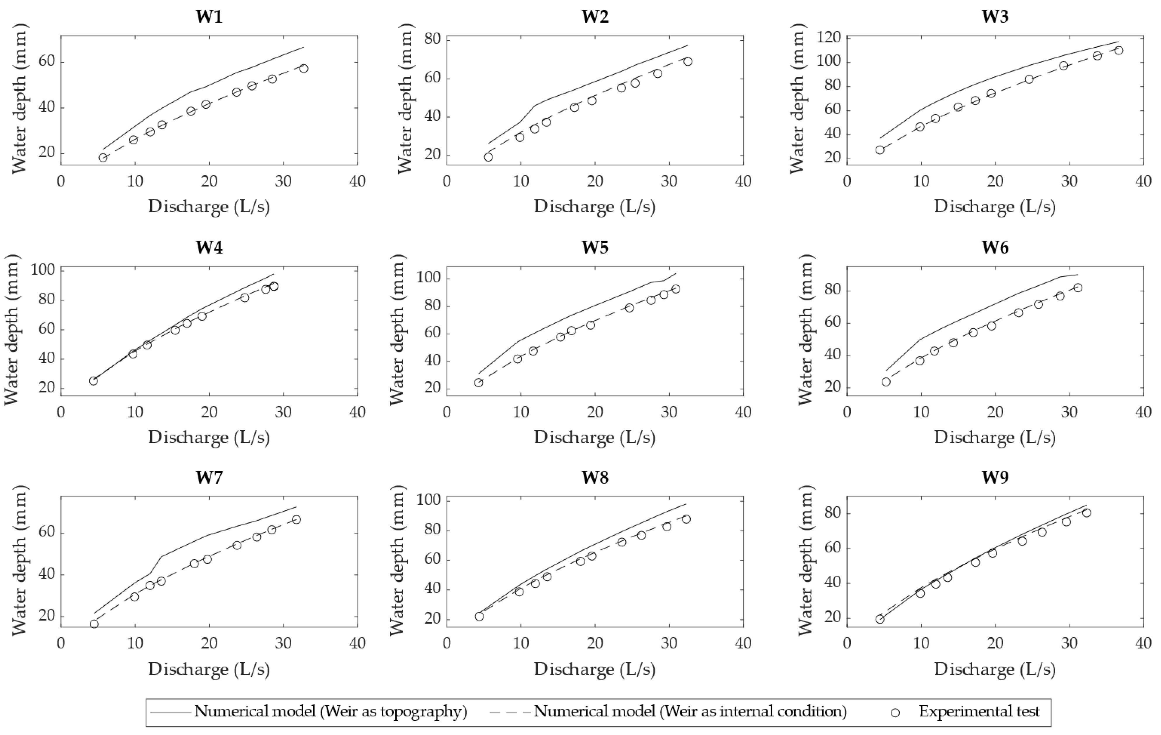
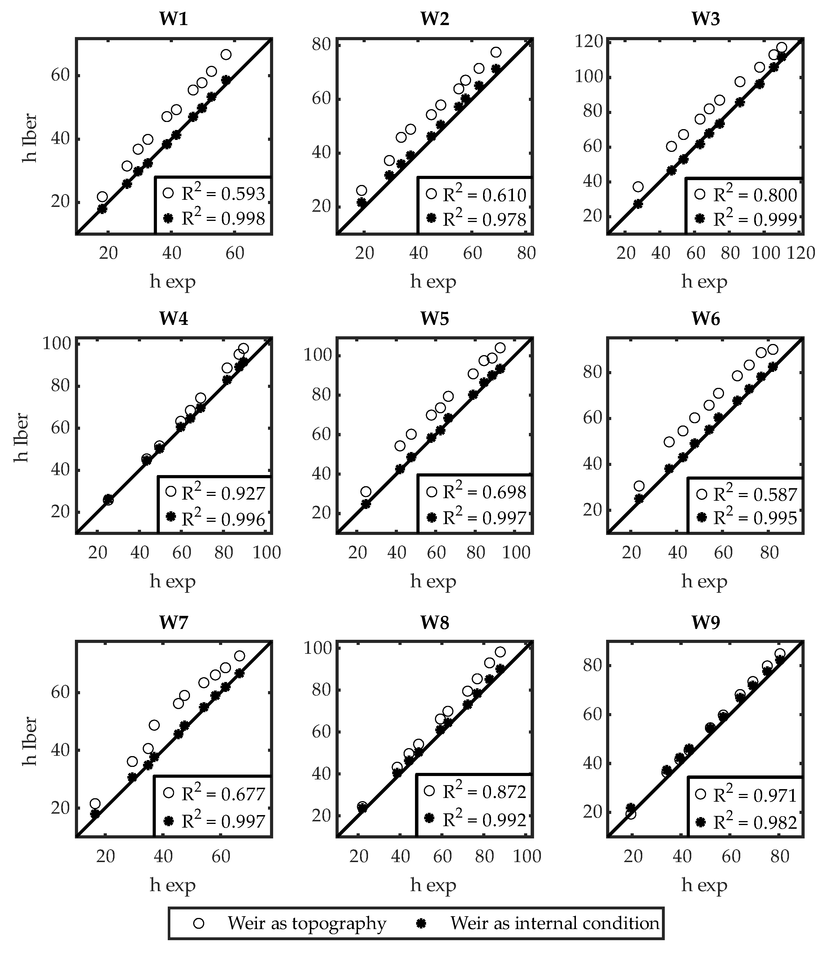
After the estimation of the Cd, the experimental tests corresponding to the first set were reproduced with the numerical model. Figure 8 compares the experimental and numerical discharge curves and Figure 9 evaluates the fit of the numerical water depth versus the experimental depth. Water depth values presented in these figures refer to the depth above the crest of the weir and measured at the control point. The numerical results include those computed modelling the weir as the model topography and as an internal condition. As can be observed, when the weir is modeled as topography, the numerical model tends to overestimate the headwater depth. On the other hand, the weir internal condition is able to reproduce the experimental data quite accurately, obtaining good results of the coefficient of determination ().
The mean absolute error (MAE) when the weir is modeled as topography varies between 4.8 and 11.4 mm (Table 3), depending on the weir geometry. These values are much higher than those obtained modelling the weir with an internal condition, where the MAE is in all cases between 0.4 and 2.4 mm.
Moreover, when the weir is modelled as the flume topography, the numerical results are more accurate in the triangular weirs (Weirs 4, 8 and 9). In those cases, the mean relative error drops to around 10%, while in the rest of the cases it remains closer to 20%. This behaviour is not observed when modelling the weirs as an internal condition.
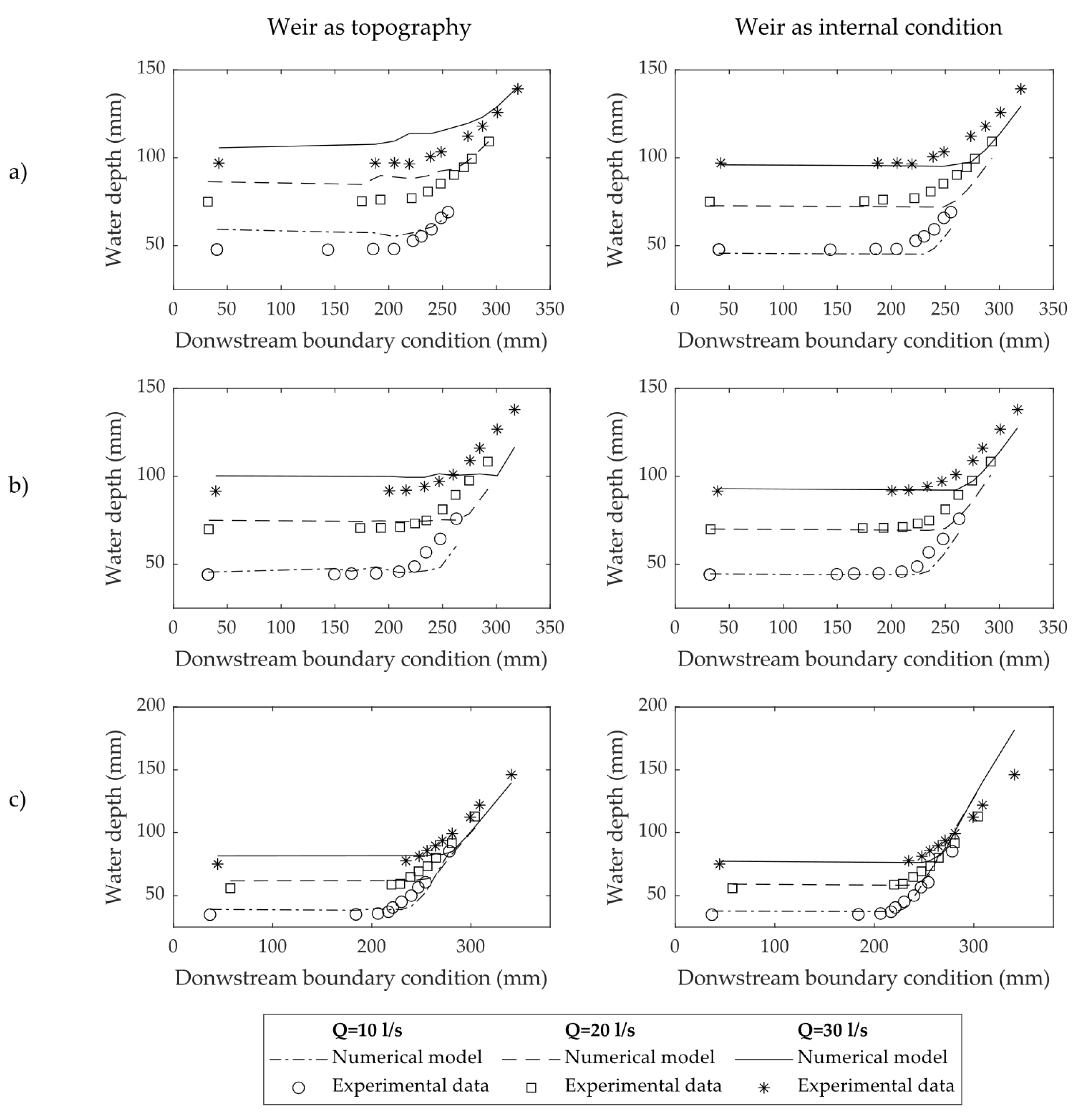
Figure 10 shows the water depth above the crest of the weirs for different downstream boundary conditions (second experimental set in Table 1). The results obtained modelling the weirs as the flume topography show a clear overestimation of the water depth when the downstream boundary condition is close to supercritical flow. This is coherent with the results of the first experimental campaign shown in Figure 8 and Figure 9. On the other hand, as the downstream water depth is increased and the weir begins to be progressively submerged, the numerical model underestimates the water depth. This is even more evident in the triangular weirs (Weirs 4 and 9).
Regarding the models with the weir modelled as an internal condition, the numerical-experimental agreement is much better when the downstream depth is low (non-submerged flow), but as the downstream water depth increases, the model begins to underestimate the headwater depth. In the particular case of Weir 9 (Figure 10c), it can be observed that the numerical-experimental differences rise sharply when the downstream boundary condition is higher than 290 mm. The experimental-numerical disagreement observed for submerged conditions could be due to the fact that the discharge coefficients used in the weir discharge equations used as internal condition (Equations (4) and (5)) were estimated experimentally for non-submerged conditions (Table 2). In order to improve the accuracy of the results, the discharge coefficients of the weirs could be re-estimated under submerged conditions, using these values in those cases where the discharge is governed by Equation (5).
4.3. Third Experimental Set
In the third experimental campaign, the spatial distribution of water depth was measured around the weirs. Figure 11 shows some representative numerical and experimental results of the spatial pattern of water depths. In general, the water depth computed with the numerical model does not represent accurately the local water depth patterns. When compared to the water depth measured in the experimental tests, the numerical model predicts very sharp gradients of the water surface elevation. The results obtained with the numerical model show a very sharp water depth drop at the weir, which is not observed in the experimental data (Figure 11a). This behaviour is even more aggravated in the weirs that are not perpendicular to the flume axis (Figure 11b). Their oblique alignment directs the water towards the side wall of the flume and generates an undular bump in the water surface elevation. This water surface pattern is not reproduced by the numerical model. In the case of Weir 9 (Figure 11c), the numerical results obtained when the weir is modelled as the flume topography are much better than those obtained by using an internal condition. Nevertheless, in the comparison of both numerical results, one must take into account the intrinsic limitations that exist in modelling a weir with slope with a one-dimensional discharge equation. This modelling approach does not correctly reproduce the flow transition between upstream and downstream.
5. Conclusions
This study presents a set of experiments of open channel flow over weirs. In total, 194 tests were carried out over nine different weir geometries in a 15 m-long flume with a 50 cm width rectangular cross-section. The headwater depth and the water depth patterns around the weirs were measured using an analog limnimeter and an automatic data acquisition system. The variety of weirs and the range of boundary conditions tested make this dataset particularly suitable for the analysis of the performance of 2D or 3D numerical models.
The experimental data were used to assess the performance and limitations of a numerical model based on the 2D shallow water equations. Two different numerical approaches to model the weirs were assessed and compared: (1) modifying the bottom topography and (2) implementing a specific internal condition for weirs.
Results show that the numerical estimations of the headwater depth are accurate when the weir is not submerged and it is modelled as an internal condition, but they deteriorate if the weir is modelled as the flume topography. This is due to the use of a constant discharge coefficient, which does not depend on the submergence conditions. In all the cases the headwater depth has been underestimated, so it would be necessary to implement a discharge coefficient dependent on the submergence conditions.
The water depth pattern around the weirs presents significant differences between the numerical and experimental results. Both numerical approaches appear to have serious difficulties in modelling the water depth pattern up- and downstream of the weirs, especially in the more complex geometries. Improvements in the estimation of the numerical model could follow two future strategies: (1) including non-hydrostatic terms in the Saint Venant 2D equations [29] and (2) coupling a 2D Saint Venant model with a 3D non-hydrostatic free surface model.
Author Contributions
Conceptualization, L.C., L.P., J.P. and G.G.-A.; methodology, L.C., L.P., J.P. and G.G.-A.; formal analysis, L.C., L.P. and J.P.; investigation, L.C., L.P. and J.P.; resources, G.G.-A., O.G.-F., L.P., L.C. and J.P.; data curation, G.G and O.G.-F.; writing—original draft preparation, G.G.-A.; writing—review and editing, L.C. and J.P.; visualization, L.C., J.P. and G.G.-A.; supervision, L.C., L.P. and J.P.; project administration, L.C., L.P. and J.P.; funding acquisition, L.C., L.P. and J.P. All authors have read and agreed to the published version of the manuscript.
Funding
This study received financial support from the Spanish Ministry of Science, Innovation and Universities (Ministerio de Ciencia Innovacion y Universidades) within the project “VAMONOS: Development of non-hydrostatic models forenvironmental hydraulics. Two-dimensional flow in rivers” (reference CTM2017-85171-C2-2-R).
Institutional Review Board Statement
Not applicable.
Informed Consent Statement
Not applicable.
Data Availability Statement
The experimental data corresponding to the tests performed in this study can be freely downloaded from the following repository: http://doi.org/10.5281/zenodo.5062775. The numerical models presented in this study are available on request from the corresponding author.
Acknowledgments
The authors would like to acknowledge the support of the group of laboratory technicians of CITEEC and the Civil Engineering School at the University of A Coruña for their collaboration in the experimental part.
Conflicts of Interest
The authors declare no conflict of interest.
Appendix A. Experimental Sets
The boundary conditions and measurements for each of the experimental sets are detailed below. In the values corresponding to experimental sets 1 (Table A1) and 2 (Table A2), the water depth values refer to the depth above the crest of the weir and were measured with the limnimeter at the control point (CP) referred in Section 4 of this article. This point is located in the central axis of the flume 700 mm away from the weir. Regarding the tests of the third experimental set (Table A3), the results detailed in this article are a summary of those obtained in the tests. The water depth value upstream and downstream of the weir refers to the average water depth of the first and last row of points measured by the automatic data acquisition system. The complete results of this last experimental set can be freely downloaded from the following repository: http://doi.org/10.5281/zenodo.5062775.

Table A1.
Experimental data corresponding to the first experimental set.
| Weir | Test | Flow Rate (L/s) | Downstream Boundary Condition | Water Depth at CP (mm) |
|---|---|---|---|---|
| 1 | 1 | 32.74 | Supercritical flow | 57.3 |
| 2 | 28.50 | 52.7 | ||
| 3 | 25.75 | 49.7 | ||
| 4 | 23.68 | 46.9 | ||
| 5 | 19.55 | 41.6 | ||
| 6 | 17.53 | 38.6 | ||
| 7 | 13.62 | 32.6 | ||
| 8 | 12.04 | 29.5 | ||
| 9 | 9.78 | 26.0 | ||
| 10 | 5.66 | 18.2 | ||
| 2 | 1 | 32.52 | Supercritical flow | 69.0 |
| 2 | 28.44 | 62.7 | ||
| 3 | 25.40 | 57.7 | ||
| 4 | 23.55 | 55.2 | ||
| 5 | 19.57 | 48.5 | ||
| 6 | 17.21 | 45.0 | ||
| 7 | 13.42 | 37.3 | ||
| 8 | 11.85 | 33.8 | ||
| 9 | 9.86 | 29.4 | ||
| 10 | 5.60 | 19.1 | ||
| 3 | 1 | 36.65 | Supercritical flow | 110.1 |
| 2 | 33.76 | 105.6 | ||
| 3 | 29.20 | 97.4 | ||
| 4 | 24.56 | 86.1 | ||
| 5 | 19.44 | 74.4 | ||
| 6 | 17.30 | 68.4 | ||
| 7 | 14.98 | 63.1 | ||
| 8 | 11.93 | 53.6 | ||
| 9 | 9.84 | 46.7 | ||
| 10 | 4.44 | 27.5 | ||
| 4 | 1 | 28.72 | Supercritical flow | 89.6 |
| 2 | 27.61 | 87.5 | ||
| 3 | 24.79 | 81.8 | ||
| 4 | 19.03 | 69.2 | ||
| 5 | 16.99 | 64.3 | ||
| 6 | 15.40 | 59.7 | ||
| 7 | 11.62 | 49.6 | ||
| 8 | 9.71 | 43.5 | ||
| 9 | 4.37 | 25.2 | ||
| 5 | 1 | 30.89 | Supercritical flow | 92.7 |
| 2 | 29.28 | 88.6 | ||
| 3 | 27.55 | 84.5 | ||
| 4 | 24.63 | 79.0 | ||
| 5 | 19.39 | 66.4 | ||
| 6 | 16.80 | 62.4 | ||
| 7 | 15.33 | 57.8 | ||
| 8 | 11.64 | 47.6 | ||
| 9 | 9.54 | 41.9 | ||
| 10 | 4.29 | 24.6 | ||
| 6 | 1 | 31.14 | Supercritical flow | 82.0 |
| 2 | 28.74 | 76.9 | ||
| 3 | 25.82 | 71.7 | ||
| 4 | 23.14 | 66.5 | ||
| 5 | 19.50 | 58.3 | ||
| 6 | 17.03 | 54.2 | ||
| 7 | 14.33 | 47.9 | ||
| 8 | 11.79 | 42.8 | ||
| 9 | 9.82 | 36.8 | ||
| 10 | 5.26 | 23.7 | ||
| 7 | 1 | 31.75 | Supercritical flow | 66.6 |
| 2 | 28.44 | 61.7 | ||
| 3 | 26.41 | 58.2 | ||
| 4 | 23.75 | 54.2 | ||
| 5 | 19.75 | 47.5 | ||
| 6 | 17.99 | 45.4 | ||
| 7 | 13.53 | 37.0 | ||
| 8 | 12.01 | 34.9 | ||
| 9 | 9.93 | 29.4 | ||
| 10 | 4.47 | 16.5 | ||
| 8 | 1 | 32.31 | Supercritical flow | 87.9 |
| 2 | 29.68 | 82.8 | ||
| 3 | 26.25 | 76.9 | ||
| 4 | 23.61 | 72.3 | ||
| 5 | 19.56 | 62.9 | ||
| 6 | 18.03 | 59.3 | ||
| 7 | 13.53 | 48.9 | ||
| 8 | 11.94 | 44.3 | ||
| 9 | 9.76 | 38.7 | ||
| 10 | 4.38 | 22.1 | ||
| 9 | 1 | 32.32 | Supercritical flow | 80.5 |
| 2 | 29.59 | 75.3 | ||
| 3 | 26.31 | 69.4 | ||
| 4 | 23.63 | 64.2 | ||
| 5 | 19.64 | 57.3 | ||
| 6 | 17.33 | 52.0 | ||
| 7 | 13.56 | 43.3 | ||
| 8 | 11.97 | 39.5 | ||
| 9 | 9.89 | 34.2 | ||
| 10 | 4.44 | 19.5 |
Table A2.
Experimental data corresponding to the second experimental set.
| Weir | Test | Flow Rate (L/s) | Downstream Boundary Condition (mm) | Water Depth 700 mm Away from the Weir (mm) |
|---|---|---|---|---|
| 3 | 1 | 9.56 | 40.3 | 47.8 |
| 2 | 143.5 | 47.7 | ||
| 3 | 185.5 | 48.1 | ||
| 4 | 204.8 | 48.1 | ||
| 5 | 222.5 | 52.8 | ||
| 6 | 230.3 | 55.3 | ||
| 7 | 239.7 | 59.3 | ||
| 8 | 248.6 | 65.8 | ||
| 9 | 255.1 | 69.1 | ||
| 10 | 19.16 | 31.9 | 75.0 | |
| 11 | 175.0 | 75.3 | ||
| 12 | 192.3 | 76.2 | ||
| 13 | 221.3 | 77.0 | ||
| 14 | 236.4 | 80.8 | ||
| 15 | 248.2 | 85.3 | ||
| 16 | 260.6 | 90.3 | ||
| 17 | 269.8 | 94.6 | ||
| 18 | 277.2 | 99.5 | ||
| 19 | 293.1 | 109.3 | ||
| 20 | 29.08 | 42.1 | 97.0 | |
| 21 | 187.4 | 97.0 | ||
| 22 | 205.3 | 97.1 | ||
| 23 | 219.1 | 96.5 | ||
| 24 | 238.7 | 100.6 | ||
| 25 | 248.7 | 103.4 | ||
| 26 | 273.5 | 112.3 | ||
| 27 | 287.1 | 118.0 | ||
| 28 | 301.0 | 125.8 | ||
| 29 | 319.9 | 139.2 | ||
| 4 | 1 | 9.82 | 32.0 | 44.1 |
| 2 | 149.5 | 44.3 | ||
| 3 | 165.4 | 44.7 | ||
| 4 | 188.3 | 44.8 | ||
| 5 | 209.5 | 45.8 | ||
| 6 | 223.9 | 48.7 | ||
| 7 | 234.6 | 56.8 | ||
| 8 | 247.9 | 64.4 | ||
| 9 | 262.8 | 75.9 | ||
| 10 | 19.36 | 32.7 | 69.9 | |
| 11 | 173.5 | 70.6 | ||
| 12 | 192.7 | 70.7 | ||
| 13 | 210.5 | 71.2 | ||
| 14 | 224.4 | 73.2 | ||
| 15 | 235.0 | 74.9 | ||
| 16 | 250.0 | 81.2 | ||
| 17 | 262.0 | 89.5 | ||
| 18 | 274.7 | 97.6 | ||
| 19 | 292.0 | 108.4 | ||
| 20 | 29.64 | 39.2 | 91.6 | |
| 21 | 200.5 | 91.8 | ||
| 22 | 216.1 | 92.1 | ||
| 23 | 233.2 | 94.2 | ||
| 24 | 246.8 | 97.1 | ||
| 25 | 259.8 | 101.0 | ||
| 26 | 275.5 | 109.0 | ||
| 27 | 284.5 | 116.1 | ||
| 28 | 300.8 | 126.8 | ||
| 29 | 316.9 | 138.0 | ||
| 9 | 1 | 10.09 | 36.8 | 34.9 |
| 2 | 184.0 | 35.1 | ||
| 3 | 206.3 | 35.8 | ||
| 4 | 216.8 | 37.2 | ||
| 5 | 221.1 | 40.6 | ||
| 6 | 230.0 | 45.1 | ||
| 7 | 239.9 | 50.1 | ||
| 8 | 246.9 | 56.7 | ||
| 9 | 254.2 | 60.7 | ||
| 10 | 278.3 | 85.4 | ||
| 11 | 19.70 | 57.4 | 56.0 | |
| 12 | 219.9 | 58.8 | ||
| 13 | 228.7 | 59.5 | ||
| 14 | 239.0 | 64.9 | ||
| 15 | 247.3 | 69.4 | ||
| 16 | 256.3 | 73.5 | ||
| 17 | 264.8 | 80.2 | ||
| 18 | 280.8 | 91.8 | ||
| 19 | 304.2 | 112.8 | ||
| 20 | 29.49 | 44.5 | 75.2 | |
| 21 | 234.5 | 77.8 | ||
| 22 | 247.8 | 81.4 | ||
| 23 | 255.8 | 85.8 | ||
| 24 | 264.2 | 89.7 | ||
| 25 | 271.2 | 93.8 | ||
| 26 | 281.2 | 99.3 | ||
| 27 | 299.2 | 112.3 | ||
| 28 | 308.8 | 121.9 | ||
| 29 | 340.9 | 146.1 |
Table A3.
Experimental data of the third experimental set.
| Weir | Test | Flow Rate (L/s) | Water Depth Downstream of the Weir (mm) | Water Depth Upstream of the Weir (mm) |
|---|---|---|---|---|
| 1 | 1 | 29.16 | 110.70 | 251.96 |
| 2 | 29.18 | 168.44 | 249.20 | |
| 2 | 1 | 29.21 | 111.80 | 262.14 |
| 2 | 28.41 | 171.85 | 260.62 | |
| 3 | 1 | 29.07 | 152.84 | 293.14 |
| 2 | 29.00 | 225.83 | 297.16 | |
| 4 | 1 | 28.03 | 146.96 | 283.10 |
| 2 | 28.29 | 229.01 | 288.80 | |
| 5 | 1 | 28.29 | 130.80 | 291.15 |
| 2 | 28.92 | 219.80 | 292.93 | |
| 6 | 1 | 29.06 | 128.93 | 273.94 |
| 2 | 28.99 | 213.08 | 277.39 | |
| 7 | 1 | 31.94 | 118.40 | 265.18 |
| 2 | 31.90 | 175.35 | 265.41 | |
| 8 | 1 | 28.90 | 134.88 | 280.54 |
| 2 | 30.47 | 210.22 | 283.68 | |
| 9 | 1 | 31.88 | 111.43 | 275.94 |
| 2 | 30.45 | 220.06 | 274.50 |
References
- Mahadevan, A.; Oliger, J.; Street, R. A nonhydrostatic mesoscale ocean model. Part I: Well-posedness and Scaling. J. Phys. Ocean. 1996, 26, 1868–1880. [Google Scholar] [CrossRef] [Green Version]
- Marshall, J.; Hill, C.; Perelman, L.; Adcroft, A. Hydrostatic, quasi-hydrostatic, and nonhydrostatic ocean modeling. J. Gephys. Res. 1997, 102, 5733–5752. [Google Scholar] [CrossRef]
- Tsai, W.T.; Yue, D.K.P. Computation of nonlinear free-surface flows. Annu. Rev. Fluid Mech. 1996, 28, 249–278. [Google Scholar] [CrossRef]
- Woodburn, J.G. Tests of broad-crested weirs. Trans. Am. Soc. Civ. Eng. 1932, 96, 387–416. [Google Scholar] [CrossRef]
- Brater, E.F.; King, H.W.; Lindell, J.E.; Wei, C.Y. Handbook of Hydraulic, 7th ed.; Mc Graw-Hill: New York, NY, USA, 1996. [Google Scholar]
- Cassidy, J.J. Irrotational flow over spillways of finite height. J. Eng. Mech. Div. 1965, 91, 155–173. [Google Scholar] [CrossRef]
- Rao, S.S.; Shukla, M.K. Characteristics of flow over weirs of finite crest width. J. Hydraul. Div. 1971, 97, 1807–1816. [Google Scholar] [CrossRef]
- Ramamurthy, A.S.; Tim, U.S.; Rao, M.V.J. Characteristics of square-edged and round-nosed broad-crested weirs. J. Irrig. Drain. Eng. 1988, 114, 61–73. [Google Scholar] [CrossRef]
- Hager, W.H.; Schwalt, M. Broad-crested weir. J. Irrig. Drain. Eng. 1994, 120, 13–26. [Google Scholar] [CrossRef]
- Gong, J.; Deng, J.; Wei, W. Discharge Coefficient of a Round-Crested Weir. Water 2019, 11, 1206. [Google Scholar] [CrossRef] [Green Version]
- Unami, K.; Kawachi, T.; Babar, M.M.; Itagaki, H. Two-dimensional numerical model of spillway flow. J. Hydraul. Eng. 1999, 125, 369–375. [Google Scholar] [CrossRef]
- Zhou, F.; Bhajantri, M.R. Numerical study of the effects of spillway crest shape on the distribution of pressure and discharge. In Proceedings of the 3rd International Conference on Hydro-Science and Engineering, Berlin, Germany, 31 August–3 September 1998. [Google Scholar]
- Bhajantri, M.R.; Eldho, T.I.; Deolalikar, P.B. Hydrodynamic modelling of flow over a spillway using a two-dimensional finite volume-based numerical model. Sadhana 2006, 31, 743–754. [Google Scholar] [CrossRef] [Green Version]
- Riha, J.; Duchan, D.; Zachoval, Z.; Erpicum, S.; Archambeau, P.; Pirotton, M.; Dewals, B. Performance of a shallow-water model for simulating flow over trapezoidal broad-crested weirs. J. Hydrol. Hydromech. 2019, 67, 322–328. [Google Scholar] [CrossRef] [Green Version]
- Dazzi, S.; Vacondio, R.; Mignosa, P. Internal boundary conditions for a GPU-accelerated 2D shallow water model: Implementation and applications. Adv. Water Resour. 2020, 137, 103525. [Google Scholar] [CrossRef]
- Cea, L.; Ferreiro, A.; Vázquez-Cendón, M.E.; Puertas, J. Experimental and numerical analysis of solitary waves generated by bed and boundary movements. Int. J. Numer. Methods Fluids 2004, 46, 793–813. [Google Scholar] [CrossRef]
- Echeverribar, I.; Morales-Hernández, M.; Brufau, P.; García-Navarro, P. Use of internal boundary conditions for levees representation: Application to river flood management. Environ. Fluid Mech. 2019, 19, 1253–1271. [Google Scholar] [CrossRef] [Green Version]
- Bladé, E.; Cea, L.; Corestein, G.; Escolano, E.; Puertas, J.; Vázquez-Cendón, E.; Dolz, J.; Coll, A. Iber: Herramienta de simulación numérica del flujo en ríos. Rev. Int. Metod. Numer. Calc. Disen. Ing. 2014, 30, 1–10. [Google Scholar] [CrossRef] [Green Version]
- García-Feal, O.; González-Cao, J.; Gómez-Gesteira, M.; Cea, L.; Domínguez, J.M.; Formella, A. An accelerated tool for flood modelling based on Iber. Water 2018, 10, 1459. [Google Scholar] [CrossRef] [Green Version]
- LeVeque, R.J. Finite Volume Methods for Hyperbolic Problems; Cambridge University Press: Cambridge, UK, 2002; ISBN 9780511791253. [Google Scholar]
- Toro, E. Shock-Capturing Methods for Free-Surface Shallow Flows; Wiley-Blackwell: Chichester, UK, 2001; ISBN 978-0-471-98766-6. [Google Scholar]
- Courant, R.; Friedrichs, K.; Lewy, H. On the partial difference equations of mathematical physics. IBM J. Res. Dev. 1967, 11, 215–234. [Google Scholar] [CrossRef]
- Cea, L.; Bladé, E. A simple and efficient unstructured finite volume scheme for solving the shallow water equations in overland flow applications. Water Resour. Res. 2015, 51, 5464–5486. [Google Scholar] [CrossRef] [Green Version]
- Cea, L.; Vázquez-Cendón, M.E. Unstructured finite volume discretisation of bed friction and convective flux in solute transport models linked to the shallow water equations. J. Comput. Phys. 2012, 231, 3317–3339. [Google Scholar] [CrossRef]
- Areu-Rangel, O.S.; Cea, L.; Bonasia, R.; Espinosa-Echavarria, V.J. Impact of urban growth and changes in land use on river flood hazard in Villahermosa, Tabasco (Mexico). Water 2019, 11, 304. [Google Scholar] [CrossRef] [Green Version]
- Bladé Castellet, E.; Cea, L.; Corestein, G. Modelización numérica de inundaciones fluviales. Ing. Agua 2014, 18, 68. [Google Scholar] [CrossRef]
- Cea, L.; López-Núñez, A. Extension of the two-component pressure approach for modeling mixed free-surface-pressurized flows with the two-dimensional shallow water equations. Int. J. Numer. Methods Fluids 2021, 93, 628–652. [Google Scholar] [CrossRef]
- Sopelana, J.; Cea, L.; Ruano, S. A continuous simulation approach for the estimation of extreme flood inundation in coastal river reaches affected by meso- and macrotides. Nat. Hazards 2018, 93, 1337–1358. [Google Scholar] [CrossRef]
- Cantero-Chinchilla, F.N.; Castro-Orgaz, O.; Khan, A.A. Vertically-averaged and moment equations for flow and sediment transport. Adv. Water Resour. 2019, 132, 103387. [Google Scholar] [CrossRef]
Figure 1.
Geometry of the weirs tested. Dimensions are shown in mm. The thickness of the stainless steel plats is 3 mm.
Figure 1.
Geometry of the weirs tested. Dimensions are shown in mm. The thickness of the stainless steel plats is 3 mm.

Figure 2.
Example of grid of measurement points at which the water depth was measured.

Figure 3.
Schematic definition of the scope of application of Equations (4) and (5).

Figure 4.
Numerical mesh used in the first and second experimental campaign (above) and in the third campaign (below). The numerical models shown in this figure corresponds to Weir 1.
Figure 4.
Numerical mesh used in the first and second experimental campaign (above) and in the third campaign (below). The numerical models shown in this figure corresponds to Weir 1.

Figure 5.
Results of the mesh convergence analysis. Water depth was measured at a reference point located 10 cm upstream of the weir in the centre line of the flume. Water depth refers to the depth above the crest of the weir.
Figure 5.
Results of the mesh convergence analysis. Water depth was measured at a reference point located 10 cm upstream of the weir in the centre line of the flume. Water depth refers to the depth above the crest of the weir.

Figure 6.
Location of the control point (CP) used in the comparisons. Weir 4 (left) and Weir 5 (right).
Figure 6.
Location of the control point (CP) used in the comparisons. Weir 4 (left) and Weir 5 (right).

Figure 7.
Theoretical adjustment of the discharge curves obtained in the experimental tests for the estimated Cd. Water depth refers to the value above the weir crest level and was measured at the control point (CP).
Figure 7.
Theoretical adjustment of the discharge curves obtained in the experimental tests for the estimated Cd. Water depth refers to the value above the weir crest level and was measured at the control point (CP).

Figure 8.
Comparison of discharge curves obtained with the numerical model (Iber) and the experimental tests (first experimental set). Water depth refers to the value above the weir crest level and was measured at the control point (CP).
Figure 8.
Comparison of discharge curves obtained with the numerical model (Iber) and the experimental tests (first experimental set). Water depth refers to the value above the weir crest level and was measured at the control point (CP).

Figure 9.
Comparison of the numerical and experimental water depth. Water depth refers to the value above the weir crest level and was measured at the control point (CP). Units in mm.
Figure 9.
Comparison of the numerical and experimental water depth. Water depth refers to the value above the weir crest level and was measured at the control point (CP). Units in mm.

Figure 10.
Comparison of the water depth result obtained by the numerical model and its corresponding value from the experimental test for Weir 3 (a), Weir 4 (b) and Weir 9 (c). Water depth measurement was taken at the control point (CP) and refers to the depth above the crest of the weir. Flow values have been simplified for the understanding of the results. The reader is referred to Appendix A for a detailed description of the test conditions.

Figure 11.
Comparison between the numerical (left and centre columns) and experimental (right column) results for Weir 3 (a), Weir 7 (b) and Weir 9 (c). Units in mm.
Figure 11.
Comparison between the numerical (left and centre columns) and experimental (right column) results for Weir 3 (a), Weir 7 (b) and Weir 9 (c). Units in mm.

Table 1.
Summary of the experimental tests.
| Experimental Set | Measuring Instrument | Weirs Tested | Upstream Boundary Condition Per Weir | Downstream Boundary Condition Per Weir | Number of Tests |
|---|---|---|---|---|---|
| 1 | Analog limnimeter | All | 10 values (9 for Weir 4) between 4 and 34 L/s | Free flow | 89 |
| 2 | Analog limnimeter | 3, 4 and 9 | 10, 20 and 30 L/s | 9 to 10 values between free flow and submerged condition 1 | 87 |
| 3 | Automatic positioner and hydraulic piston | All | 30 L/s | Free flow and partially submerged condition | 18 |
1 Depending on the geometry and the inlet discharge, between 9 and 10 downstream boundary conditions were established from free flow condition to submerged condition (see Appendix A for details).
Table 2.
Estimated discharge coefficient for each of the weirs.
| Weir | Cd |
|---|---|
| 1 | 1.81 |
| 2 | 1.75 |
| 3 | 1.99 |
| 4 | 2.13 |
| 5 | 1.91 |
| 6 | 1.87 |
| 7 | 1.83 |
| 8 | 2.11 |
| 9 | 1.95 |
Table 3.
Mean relative error (MRE), mean absolute error (MAE) and root mean square error (RMSE) values of the numerical models in the comparison with the data obtained at the first experimental campaign.
Table 3.
Mean relative error (MRE), mean absolute error (MAE) and root mean square error (RMSE) values of the numerical models in the comparison with the data obtained at the first experimental campaign.
| Weir | Weir Modeled as Topography of the Flume | Weir Modeled as Internal Condition | ||||
|---|---|---|---|---|---|---|
| MRE 1 (%) | MAE (mm) | RMSE (mm) | MRE 1 (%) | MAE (mm) | RMSE (mm) | |
| 1 | 19.6 | 7.5 | 7.7 | 0.9 | 0.4 | 0.5 |
| 2 | 22.9 | 9.3 | 9.4 | 5.6 | 2.2 | 2.2 |
| 3 | 18.3 | 11.1 | 11.4 | 1.0 | 0.7 | 0.9 |
| 4 | 6.4 | 4.5 | 5.2 | 1.9 | 1.1 | 1.2 |
| 5 | 19.5 | 11.4 | 11.6 | 1.6 | 1.0 | 1.2 |
| 6 | 22.1 | 11.2 | 11.4 | 2.4 | 1.2 | 1.3 |
| 7 | 20.0 | 8.2 | 8.5 | 2.1 | 0.7 | 0.8 |
| 8 | 11.3 | 6.8 | 7.2 | 3.3 | 1.7 | 1.8 |
| 9 | 5.0 | 2.9 | 3.2 | 5.5 | 2.4 | 2.5 |
1 To calculate the mean relative error (MRE), the absolute error at each measurement point was divided by the water depth above the crest of the weir at the same location.
Publisher’s Note: MDPI stays neutral with regard to jurisdictional claims in published maps and institutional affiliations. |
© 2021 by the authors. Licensee MDPI, Basel, Switzerland. This article is an open access article distributed under the terms and conditions of the Creative Commons Attribution (CC BY) license (https://creativecommons.org/licenses/by/4.0/).
Share and Cite
MDPI and ACS Style
García-Alén, G.; García-Fonte, O.; Cea, L.; Pena, L.; Puertas, J. Modelling Weirs in Two-Dimensional Shallow Water Models. Water 2021, 13, 2152. https://doi.org/10.3390/w13162152
AMA Style
García-Alén G, García-Fonte O, Cea L, Pena L, Puertas J. Modelling Weirs in Two-Dimensional Shallow Water Models. Water. 2021; 13(16):2152. https://doi.org/10.3390/w13162152
Chicago/Turabian StyleGarcía-Alén, Gonzalo, Olalla García-Fonte, Luis Cea, Luís Pena, and Jerónimo Puertas. 2021. "Modelling Weirs in Two-Dimensional Shallow Water Models" Water 13, no. 16: 2152. https://doi.org/10.3390/w13162152
Note that from the first issue of 2016, this journal uses article numbers instead of page numbers. See further details here.