
Classification of Aquifer Vulnerability by Using the DRASTIC Index and Geo-Electrical Techniques
by
 , , ,
, , ,
Syed Hassan Iqbal Ahmad Shah
1, 
Jianguo Yan
1,
Israr Ullah
2 ,
,
Bilal Aslam
3,
Aqil Tariq
1,*,† ,
,
Lili Zhang
4,5,*,† and
Faisal Mumtaz
6,7
1
State Key Laboratory of Information Engineering in Surveying, Mapping and Remote Sensing, Wuhan University, Wuhan 430072, China
2
Neotectonis and Natural Hazards, RWTH Aachen University, Locknerstr, 4-20, 52056 Aachen, Germany
3
Department of Data Science, Riphah International University, Islamabad 45210, Pakistan
4
Aerospace Information Research Institute, Chinese Academy of Sciences, Beijing 100101, China
5
Zhongke Langfang Institute of Spatial Information Applications, Langfang 065001, China
6
State Key Laboratory of Remote Sensing Sciences, Aerospace Information Research Institute, Chinese Academy of Sciences, Beijing 100101, China
7
University of Chinese Academy of Sciences (UCAS), Beijing 101408, China
*
Authors to whom correspondence should be addressed.
†
These authors contributed equally to this work.
Water 2021, 13(16), 2144; https://doi.org/10.3390/w13162144
Submission received: 28 June 2021
/
Revised: 30 July 2021
/
Accepted: 30 July 2021
/
Published: 4 August 2021
(This article belongs to the Special Issue Protection and Usage of Groundwater)
Abstract
:Vulnerability analysis in areas vulnerable to anthropogenic pollution has become a key element of sensible resource management and land use planning. This study is intended to estimate aquifer vulnerability using the DRASTIC model and using the vertical electrical sounding (VES) and electrical conductivity (EC) outcomes. The model allows for the identification of hydrogeological environments within the scope of the research, based on a composite definition of each environment’s main geological, geoelectrical, and hydrogeological factors. The results from the DRASTIC model were divided into four equal intervals, high, medium, low, and very low drastic index values. The SW area and NE area depict drastic index values from medium to very high, making it the most vulnerable zone in the study area, while the NW and SW areas show low to very low drastic index values. In addition, the results from the VES and EC the freshwater aquifer in the NE area and brackish water in the SE area, while the rest of the area falls into the category of brackish water. Overall, it can be concluded that areas having freshwater assemblages are on the verge of becoming contaminated in the future while the rest of the NW and SW areas constitute less vulnerable zones. The validation conducted for DRASTIC and EC shows a nearly positive correlation. Wastewater treatment policies must be developed throughout the studied region to prevent contamination of the remaining groundwater.
1. Introduction
Groundwater is the world’s most valuable resource. It makes up about 90% of humanity’s freshwater supply and supplies about one third of the world’s consumption of water. However, groundwater water is profoundly vulnerable to contamination [1]. The contamination of groundwater has become a prevailing problem throughout the world. When groundwater is contaminated it becomes difficult to remediate, despite its self-remediation capacity. As a result, sustainable groundwater management should be centered on pollution prevention. Before considering strategies to prevent future groundwater quality issues, groundwater conditions (and especially the type of recharge) should first be determined for the aquifer [2]. Groundwater contamination can still be hard to identify and control for many years and perhaps decades.
Groundwater quality is as important as quantity. It can be affected by many factors or seriously deteriorated. These factors include a rapid rise in urbanization, mixed land use designs, the lack of an appropriate sewage framework, advanced agricultural production, and poor disposal of wastewater. These can be caused by household as well as industrial activities and can introduce pathogens, heavy metals, trace elements, organic chemicals, nitrates, pesticides, herbicides, fertilizers, and hydrocarbons into groundwater systems. These pollutants result in increased waterborne diseases, including gastrointestinal illness, cholera, typhoid, amoebiasis, hepatitis A, and diarrhea [3]. In developing countries such as Pakistan, nearly 66% of water is provided by hand-pumps and piped system [4]. Inferior quality drinking water accounts for 30% of maladies and 40% of all deaths [5]. According to an assessment, over 0.1 million Pakistanis die, and about three million people are affected, by waterborne illness every year [6]. In different areas of Punjab, the majority of the populace is deprived of clean drinking water.
The assessment of groundwater vulnerability to pollution has been extensively used worldwide by researchers. The term “vulnerability of groundwater to contamination” was first utilized by Margat in 1968 [7]. Groundwater vulnerability is defined as the tendency and probability of a contaminant to reach the groundwater table after originating at the ground surface [8]. Worldwide planners and researchers concede that there is a need for figuring out proficient and effective strategic plans. Therefore, developing a framework to improve available water assets and secure them quantitatively and qualitatively is very important.
There are three methods for accessing the vulnerability of groundwater to pollution, namely process-based methods [9], statistical methods [10], and overlay and index methods [11]. A processed-based method uses numerical modeling to estimate the contaminant transport. It is limited by poor accessibility of adequate data and often faces computational challenges [12]. A statistical method involves comparing spatial variables with actual water quality data and uncertainty. It attempts to reduce errors and utilize parameter coefficients rather than weight [3]. Maps of the parameters which influence contaminant transfer between surfaces and groundwater must be compiled and combined for the overlay and index method. This then has an index value. Moreover, this method is easy to deploy. This method is the most suitable technique for the assessment of groundwater vulnerability and is the result of rapidly accessible data and subjective assessment. Ordinarily, overlay and index models include EPIK [13], GOD [14], AVI [15], SINTACS [16], and DRASTIC [17]. Among them, the DRASTIC is the most popular and widely used approach [18].
Using the DRASTIC and GIS method together is effective in evaluating aquifer vulnerability. The DRASTIC model was given by [17], in combination with the US Environmental Protection Agency and the National Water Well Association. Groundwater flow controls the geological and hydrological features of an area. Seven hydrogeological parameters are included in the DRASTIC model. These parameters constitute acronyms that form the term “DRASTIC” and include depth to the water table, recharge of network area, aquifer media, soil media, topography, the impact of the vadose zone, and hydraulic conductivity [19]. The DRASTIC function evaluates the area in various vulnerability zones built on DI (DRASTICIndex) [20].
For this research, the region of Safdarabad Tehsil, the Punjab district of Sheikhupura, Pakistan was selected. This area is irrigated by an alluvial arrangement via canal water. Sheikhupura is an industrial city. The study area does not belong to the coastal region and, as part of Rachna Doab, is the reason for incorporating the DRASTIC method in our study. Gillani et al. 2013 [21] studied the groundwater quality of tehsil Sheikhupura. Their results from drinking water samples illustrate that four out of twelve sites have an elevated amount of bacterial contamination, manganese, and arsenic level, while three samples have higher sulfate amount than the WHO limit due to sulfate fertilizers usage. Previously, [22] has conducted GIS-based drastic analysis in the same region for a bigger area. The limitation of that work was that there was no availability of geophysical data for the sake of comparison. However, in the current study we have acquired geophysical data and aim to compare it with the DRASTIC results in order to determine areas having a fresh water interface. In this way, the accuracy of the DRASTIC analysis can be tested and proper groundwater mitigation and planning can be developed as well. In the last decade, there has been a significant increase of the use of geophysical methods for the characterization of hydrogeological sites [23]. Geophysical techniques were used by many authors to solve concerning hydrogeological issues [24]. This technique has also been utilized by many authors for vulnerability mapping and studies [2,3,4]. It is a non-invasive, nature-friendly, and economic technique [25]. For the current study, the VES data are provided from the district agricultural department. Electrical Conductivity (EC) data of groundwater samples from the nearby tube wells of the VES points have also been obtained to find out the groundwater contamination [26]. However, for detailed lithological classification, one cannot completely rely on the VES results due to overlapping of the resistivity of the subsurface layers. For better interpretation, its comparison with borehole data is important to verify the output. For DRASTIC, its capability and usability represent a common approach used to evaluate the vulnerability of groundwater. DRASTIC index-based techniques are not related to data access or similarities. The key advantage of GIS is the combined efficiency of data layers and a modification of vulnerability classification parameters. The limitations of the DRASTIC technique are that it cannot measure and identify pollutants, but instead can only estimate the infiltration and stability capacity of the aquifers.
The current research focuses on two aspects. First, we focus on the DRASTIC model and GIS techniques to be used in order to identify contamination-prone areas and classify vulnerability zones. Secondly, we focus on the VES and EC approach for the sake of comparison, correlation, and validation with the DRASTIC method. This study will help us to identify fresh groundwater sources that are on the verge of getting contaminated.
2. Materials and Methods
2.1. Study Area
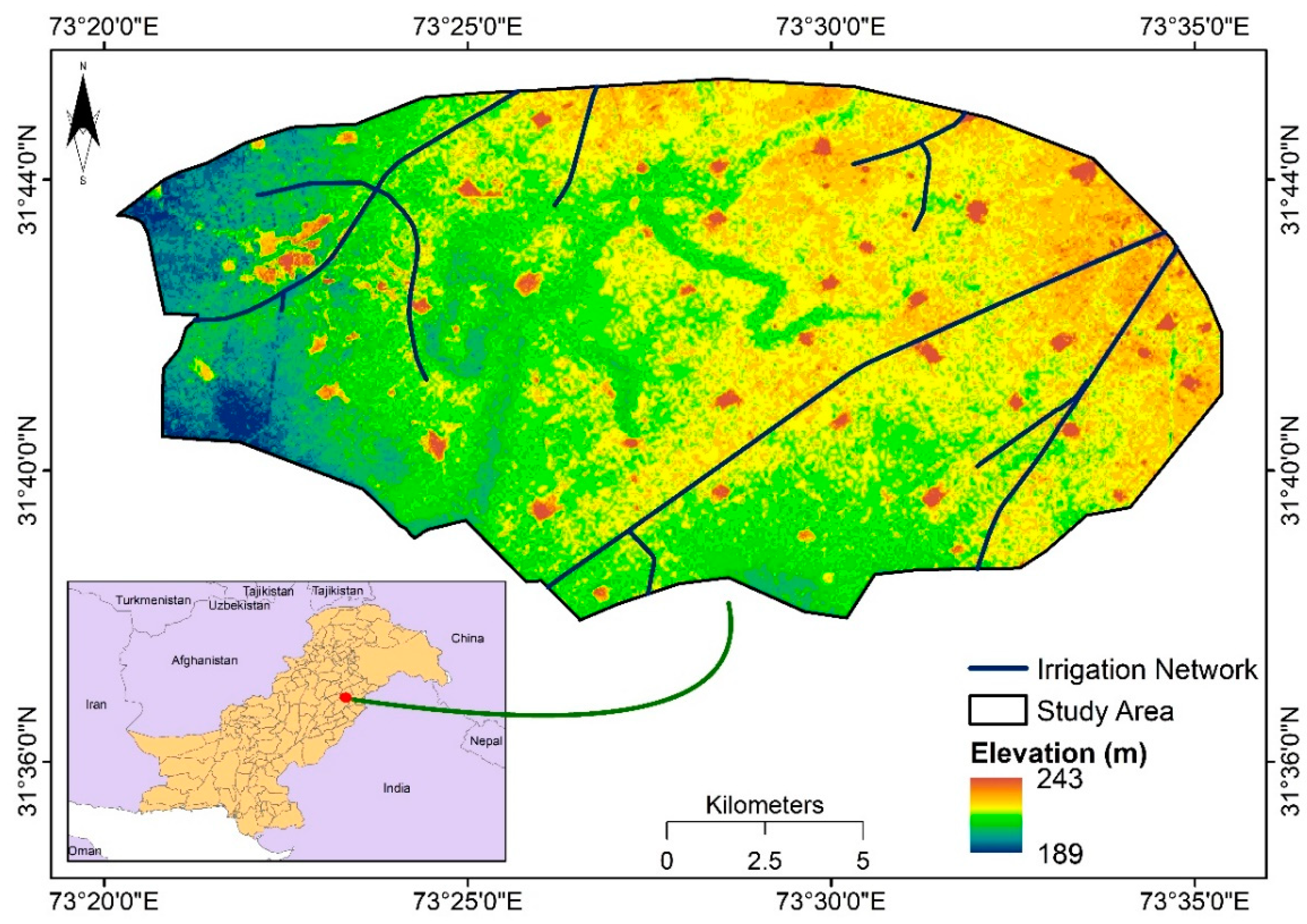
The area, Safdarabad Tehsil, in our investigation in which the DRASTIC model and the VES technique were applied is situated on the northeast side of Punjab. It lies between longitude 73°37′45.60″ E to 74°7′39.52″ E and latitude 31°58′55.22″ N to 31°29′44.07″ N (Figure 1). The region is encircled by the River Chenab on the western side and the River Ravi on the eastern side. Safdarabad Tehsil is a part of Rachna Doab. The total explorative area of Safdarabad Tehsil is 134.3 km2. Sand storms occasionally occur in the area. The precipitation is 500 mm/year. The summer season starts from April and continuous until October with a temperature range from 30 to 45 degree Celsius. The coldest temperatures reach at least a median temperature of 5 degrees in winter (between December and January). The area consists of alluvial sediments, and these alluvial sediments are derived from rivers from the Himalayas in the northern area under investigation [27]. The River Chenab shaped most of the investigative zone topography. The geology of Safdarabad is composed of aeolian and thick alluvium deposits of dynamic flood plains and pediment deposits of the quaternary period. In comparison to the surface runoff, the capacity for water to enter the soil is higher. The stream direction of groundwater is south-east [28].
2.2. Dataset
The DRASTIC model is an empirical model that assesses the vulnerability of the groundwater system centered on in situ hydrogeological data [29]. It can be used in large areas due to its simple nature and low cost of application. The DRASTIC method is an intrinsic vulnerability evaluation method for the common point count system model (PCSM) and the parameter weighting method [16]. This methodology uses the following set of seven hydrogeological parameters: depth to the water table, net recharge, aquifer media, soil media, topography, the impact of the vadose zone, and hydraulic conductivity. These parameters have been divided into different ranges, and each parameter has been assigned rating and weights. Relative weight was given by factors with regard to each other in accordance with numerical scale 1–5 and showed the importance of each parameter. The most vulnerable parameter is demonstrated by a higher value, while the least vulnerable is indicated by a lower value. The range for an individual parameter was allotted a subjective rating. The rating for each DRASTIC parameter was carried between 1 and 10. The most vulnerable range of a parameter is reflected by a higher rating value [17,29]. The DRASTIC model was utilized to yield a numerical index by summing up the product of ratings and weights for seven parameters [30,31]. The final vulnerability map is based on a DRASTIC Index (DI), which is computed by using Equation (1) [30]:
where r and w denote the rating and weight, respectively (assigned to each parameter), D is the depth to the water table, R is the recharge of network area, A is the aquifer media, S is the soil media, T is the topography, I is the impact of the vadose zone, and C is the hydraulic conductivity. A large DRASTIC index value indicates an increase in the probability of aquifer contamination.
To find the groundwater recharge technique implemented from [32], the following Equation (2) is used:
By adding base flow component of the run-off to the net recharge, the gross recharge can be calculated. This method is more reliable since the involved parameters can be calculated more precisely and accurately than other parameters such as evaporation and evapotranspiration. The water level fluctuation height between post-monsoon and pre-monsoon seasons is of more significance than the annual water level fluctuation height for groundwater development and management purposes. These values therefore depict the effective recharge of groundwater due to rainfall [32].
Background Sources and Preparation of Input Datasets
This study was based on GIS techniques to prepare and integrate data layers and classify the vulnerability of the basin. The seven layers were converted to raster data using ArcGIS after being converted into a compatible digital format and calibrated using the WGS84-UTM coordinate system. All of the layers were classified, with relative rates and weights allocated to each. The DI was then calculated, and the vulnerability map was generated using hydrological field observations and investigations. The vulnerability maps are the final results and indicate which areas of contaminated groundwater are more likely to be contaminated than others. In Table 1, the input parameter map data sources are shown.
2.3. Vertical Electrical Sounding
Vertical Electric Sounding is a technique which uses direct current. In this method, two current electrodes are injected into the ground and their potential is then detected by two potential electrodes [33]. The array used for groundwater studies is the Schlumberger array. In the Schlumberger array, the spacing between electrodes is directly related to the depth of investigation [34]. The spacing between the electrodes for the current study was 300 m. The depth of investigation for the current area can be marked as AB/4, as explained in the previous work done by [35] in the neighboring areas of the current study area. Thus, the depth of investigation for the current region will be 75 m. The VES data is processed by using IPI2WIN software, which gives the true resistivity values and the thickness and depth of subsurface layers [36]. The software produces the subsurface resistivity curves which gives us information about the true resistivity variation with the increase in depth.
The true resistivity values obtained after IPI2W processing are used for deriving the Dar Zarrouk (DZ) parameters [37]. The DZ parameters help to identify the areas having saline groundwater in the area [24]. The DZ parameters are defined in terms of transverse resistance and longitudinal conductance. The longitudinal resistivity is also derived using these values [38,39]. The transverse resistance is denoted by Tr and longitudinal resistivity is denoted by ρL. The units of DZ parameters are Ωm2, mho and Ωm respectively.
In which h is the thickness of the layer and ρ is the true resistivity of the layer, the longitudinal conductance is denoted by Sc, and is the total thickness of the layers. The pseudo cross-section and resistivity cross-section are produced in the IPI2WIN software for interpreting the subsurface lithology.
2.4. Electrical Conductivity (EC) and Total Dissolved Solids (TDS)
Due to the varying behavior of resistivity of subsurface material depending on the injected current, the VES result cannot provide reliable results for groundwater exploration. Various materials show varying resistivity to the injected current. This is the reason EC samples of the freshwater from nearby tube wells need to be collected [25]. Both the values of EC and TDS are used to identify the fitness of water for drinking and irrigation purposes [40]. The EC data was measured by using a portable EC and TDS meter [41]. The EC values were used in Equation (5) to get the total dissolved solids (TDS):
The EC value will be multiplied by 0.64 if it is in μS/cm, and it will be multiplied by 640 if it is dS/m [25,39]. When the EC values are at least 5 μS/cm, Equation (5) will be used. The accuracy assessment of this equation has been done [42] with a proper comparison of these results with laboratory measurements. This is why this equation can be utilized to obtain the TDS.
3. Results
3.1. The DRASTIC Parameters
The seven thematic maps are produced as a raster grid. The DRASTIC values rates and weights for the study region are shown in Table 2. These rates and weights were well defined by the Delphi method [43] and are used globally [44]. The scale of risk established is generic rather than site-specific. The following features are included in the DRASTIC parameters.
Table 2 shows the interval, weight, DRASTIC, and consequent water depth index. The water table depth is very important in terms of determination of the factors influencing groundwater vulnerability against pollutants since it is basically the indicator of the distance needs to be covered before inflowing to an aquifer. Table 2 demonstrates the proportional importance of water depth [45]. Lower ratings thus indicate deeper and less contaminating groundwater levels [18].
3.1.1. Depth to Water Table
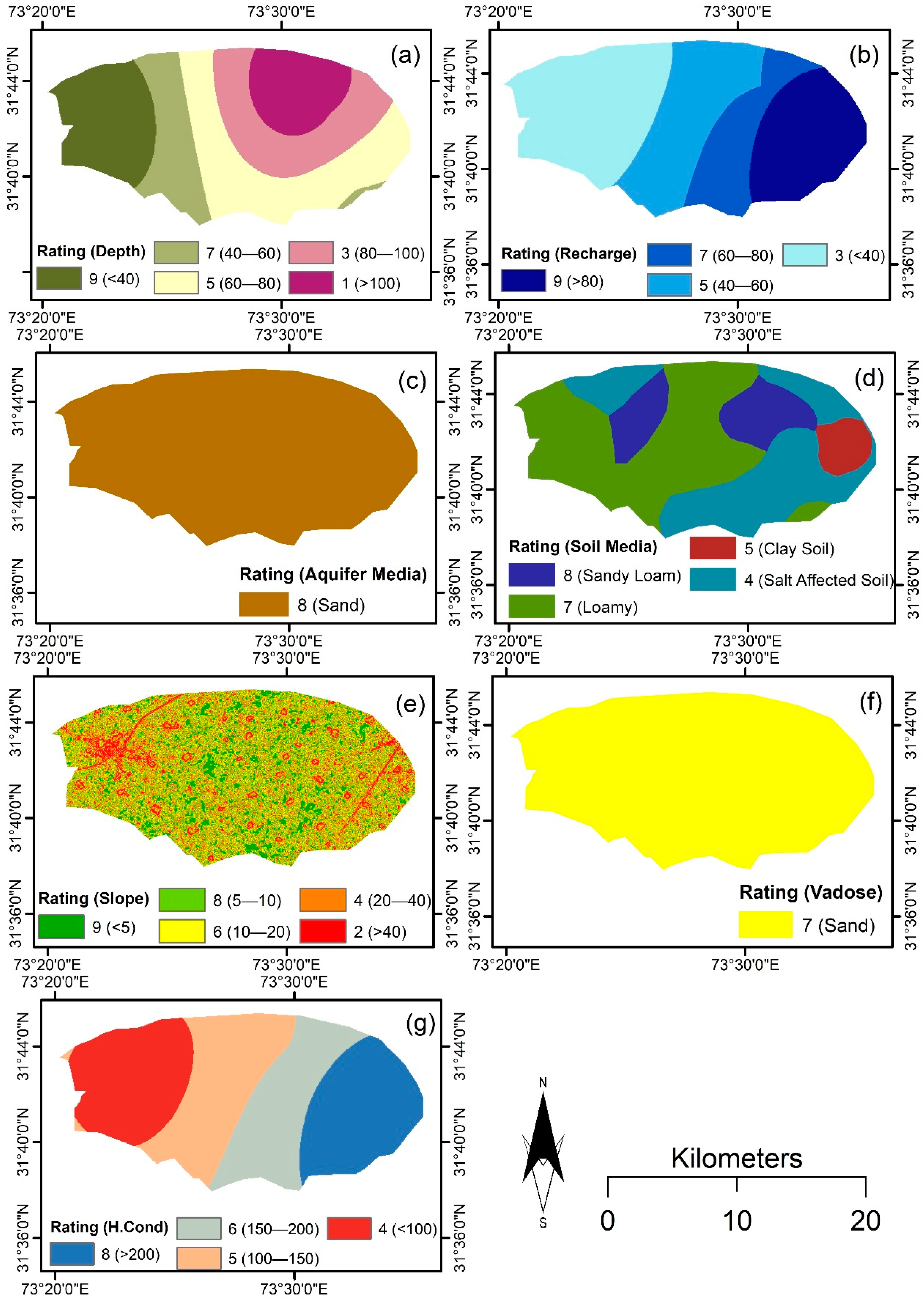
The profile of the water table refers to the distance between the ground surface and the water table. It is a key parameter and defines the extent of a medium by which the water infiltrating, or percolating must move before reaching the water that is soaked [47]. For a deeper water table, the processes of diminution can be implemented to eliminate the contamination by providing the contaminated water with soil media with an adequate elapsed time. The depth to water table was acquired from randomly distributed eight wells in our study area and kriging interpolation was used. The groundwater level in Safdarabad Tehsil varies from depth of under 40 m in the sub-surface to a depth of more than 100 m, as portrayed in depth to water table map (Figure 2d). It has been allotted a maximum weight of five according to [48]. It is then reclassified into five classes (<40, 40–60, 60–80, 80–100, and >100) and assigned a rating of 9, 7, 5, 3, and 1, respectively. Table 2 shows the interval, rating, and weight of the water table depth. Due to the shorter distance involved in travelling before reaching the water table, the shallow water table zone is vulnerable to pollutants. Thus, the higher the water table the higher the value. Table 1 shows the drastic parameters together with their scope, rating and weight.
3.1.2. Net Recharge
Net recharge refers to the amount of water flowing through the water table. In the movement of groundwater pollution, it plays an essential role. Safdarabad lies between the east of the Ravi River and the west of the Chenab River. The aquifer is recharged from the rivers Chenab and Ravi, where the river Chenab is the main contributor to the water recovery. Net recharge would ease the migration of pollutants to spread to the water table under the influence of gravitational force. The dilution and dispersal of pollutants rely significantly on net recharge. For this reason, a greater net recharge corresponds to a higher vulnerability to groundwater contamination. Net recharge values were acquired from water tables data and the kriging interpolation method was used. Net recharge was given a maximum weight of four and was categorized into four classes (<40 mm/year, 40–60 mm/year, 60–80 mm/year, and >80 m/year) and were assigned a recharge rate of 3, 5, 7, and 9, respectively. The net recharge is charted and shown in Figure 2b.
3.1.3. Aquifer Media
A body of saturated rock is defined as an aquifer providing significant amounts of water to be used. The aquifer media refers to the unconsolidated rock with its capacity to store water [49]. The aquifer medium monitors the flow rate, nature and contaminant contact rate in the aquifer and give valuable insight into the likelihood that a reduction of the contamination process will occur. The aquifer containing larger grain size, high void ratio, and more fractures have higher permeability which results in lower pollutant attenuation capacity that, being so, leads to greater contamination potential [50]. Thus, the coarser medium was given a higher rating value. The only lithological component in the exploration area of the aquifer is sand (which is 8) and the weight of the aquifer media (which is 3), as shown in Table 2. It has been portrayed in Figure 2f.
3.1.4. Soil Media
Soil media is considered the uppermost weathered portion over the vadose zone [17]. This has a major impact on the quantity of recharge and the transport of contaminants into the groundwater. Silt and clay materials with finely textured materials have lower relative soil permeability with a delayed contaminant migration [46]. The region under investigation comprises alluvial soil brought from the Himalayan Mountains by the rivers. Four types of soil found in our study include salt-affected soil, clayey soil, loamy and sandy loam having ratings of 4, 5, 7, and 8, respectively, and were assigned a total weight of 2. Their visual presentation is illustrated in Figure 2a.
3.1.5. Topography
The slope and slopes availability of an area are referred to as topography. The topography determines the rate of surface runoff or contaminant residence time on the ground needed for the entrance into the saturated zone [48]. DEM for the study area had been acquired for the topography of the intended area. Areas with mild slopes tend to reduce surface runoff capacity, increase the likelihood of containment infiltration, and increase the vulnerability to groundwater pollution. The ratings have been allocated on a standardized scale of 1–10, with 10 assigned to the lowest slope and 1 assigned to the highest slope as indicated in Table 2. The topology is divided into five classes (<5, 5–10, 10–20, 20–40, and >40) with ratings of 9, 8, 6, 4, and 2, respectively. Topography has been given a weight of 1, as shown in Figure 2e.
3.1.6. Impact of Vadose Zone
The vadose zone is the unsaturated surface layer above the water table. This layer has an enormous impact on the groundwater pollution potential. Vadose zone effects are a complex factor in controlling various physiochemical processes. The attenuating properties are also based on material type in the vadose area and play an essential role in reducing groundwater contamination [3]. The material forming the vadose zone of the pertaining area constituted sand only and was assigned a rating of 7. The allocated weight for vadose zone is 5 as shown in Figure 2g.
3.1.7. Hydraulic Conductivity
The aquifer’s potential for water transmission is measured by hydraulic conduction. It controls the flow of groundwater, which controls the contaminant’s movement within the aquifer. The saturation, intrinsic permeability, viscosity and material density depend on this. An aquifer having high hydraulic transmission is more vulnerable to groundwater contamination. Hydraulic conductivity was acquired from the borehole data. A weight of 3 was assigned. In four classes were categorized in the hydraulic values found in the area of study: <100 m/d, 100–150 m/d, 150–200 m/d, and >200 m/d. The grades for hydraulic conductivity in Figure 2c were 4, 5, 6, and 8, respectively.
3.2. DRASTIC Vulnerabilty Map
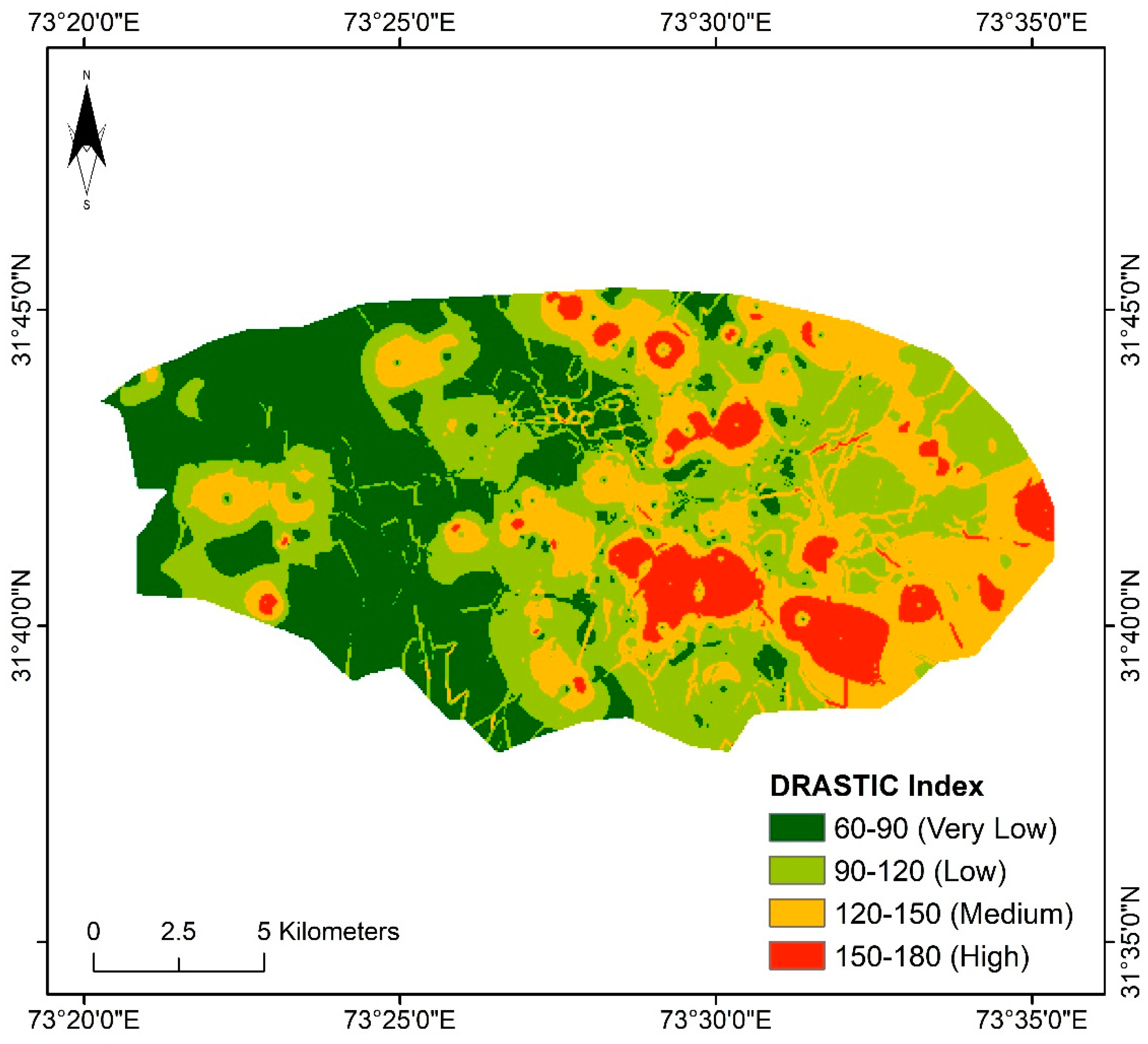
The input layers were integrated into a single DRASTIC risk map (Figure 3) to visualize which areas in the Safdarabad area are more vulnerable to groundwater contamination.
In Figure 3, we can see that in the south, southeast, and northeast, the study region is highly vulnerable to pollutants. The groundwater vulnerability is classified into four categories using the equal interval method based on their DI (DRASTIC Index) value. The DI ranges from 60 to 180. The 60–90 DI values point to the lowest risk area, the 90–120 DI to the low vulnerability area, 120–150 to a medium vulnerability area, and 150–180 to the highest risk area. The higher indices reflect the higher relative potential of contamination. The NE and SE areas are shown to be high values of the drastic index. This may also be due to the presence of a recharge source in that area, which can increase hydraulic conductivity and infiltration to the aquifers. This situation can be tackled by the proper implementation of wastewater treatment policies in the area to save the precious fresh quality groundwater.
3.3. Interpretation of VES results
The VES data have been interpreted by using the geo-electrical parameters to identify the saline water zone. The threshold values for these parameters in the current study area are given by [25]. The groundwater will be saline if Tr < 700 Ωm2 and ρL < 15 Ωm. The groundwater will be brackish if the values lies between Tr from 700 to 1700 Ωm2 and ρL between 15 and 25. The freshwater is marked as having Tr > 1700 Ωm2 and ρL > 25 Ωm. The geo-electrical parameters of our study area are presented in Figure 4.
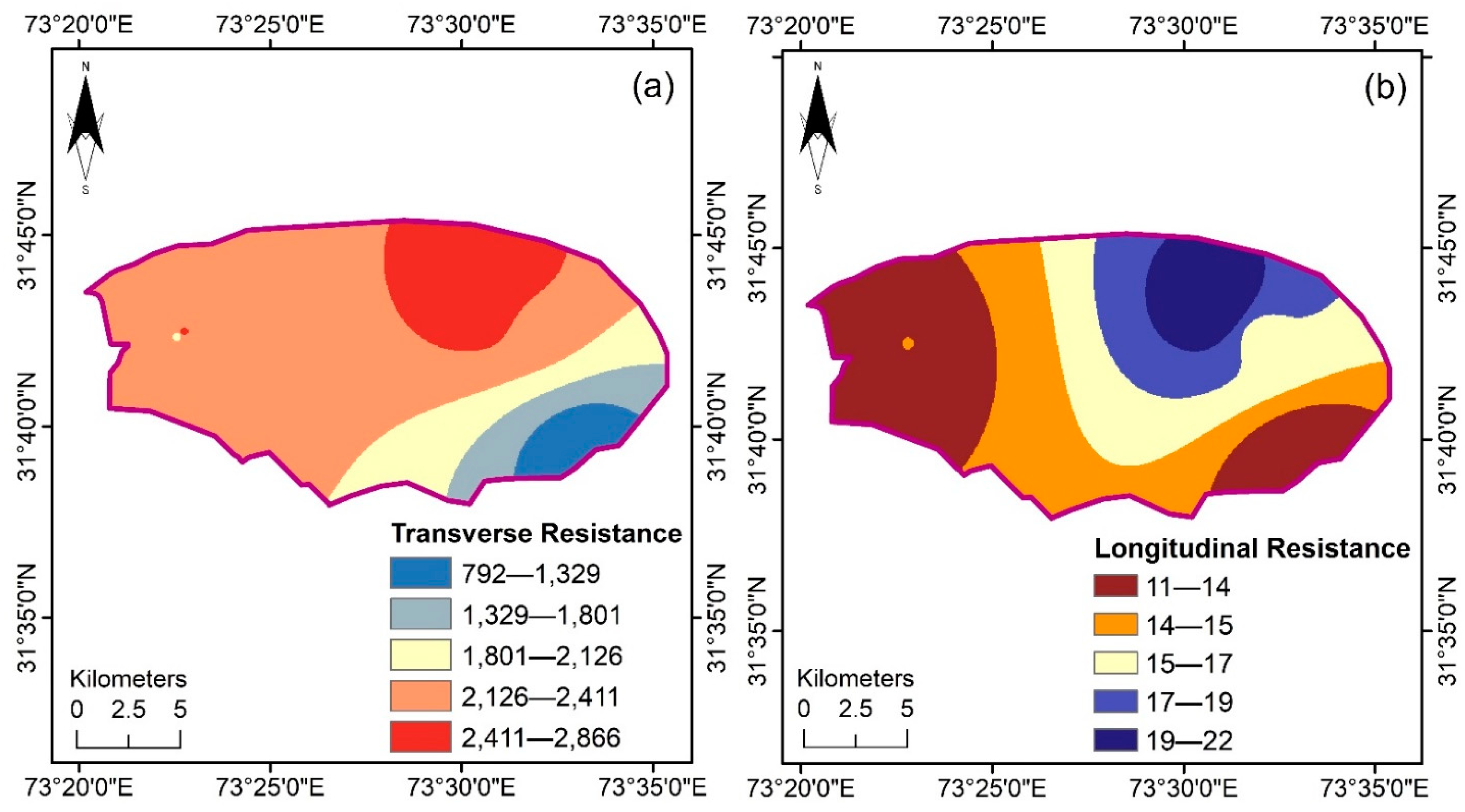
As shown in Figure 4a, the Tr shows the highest peak in the NE area, while Tr values in the central and western areas are also high. In the SE area, the transverse resistance has the lowest values indicating brackish water. From Figure 4b, we can find that the highest values of longitudinal resistivity between 15 Ωm and 25 Ωm lie in the NE and northern area, while the south-central and SW area show saline water zone as having longitudinal resistivity values less the 15 Ωm.
3.4. Cross-Section Analysis
With the help of cross-section analysis, the subsurface lithology trend can be studied. Khalid et al. (2019) has deduced the criteria to interpret the lithology. Referring to [51,52], a set of specific values for every different type of lithology was defined as in Table 3.
The hydrogeological conditions of the test area, as shown in Table 3, were used to calibrate resistivity and lithology. The modeled VES curves were tuned and interpreted using knowledge from the study area’s geology and borehole lithology. Depending on moist conditions, sand resistivity is often greater than clay resistivity. Similarly, gravel resistivity is greater than sand resistivity [53]. The pseudo cross-section of the area is prepared by using the IPI2WIN software and is shown in Figure 5. It provides an opportunity to visually analyze the subsurface variations in the true resistivity.
3.5. EC and TDS Variation in the Area
The EC variation obtained from groundwater samples was recorded. The TDS was also obtained by using Equation (5). However, the TDS values are only an estimation. The detailed comparison of the TDS values obtained by Equation (5) with laboratory measurements is made previously [26,43] with a 10 percent of accuracy. Table 4 gives the degree of restriction for a quality water based on the EC and TDS measurements.
According to the guidelines in Table 4, the study area shows two general areas. One area has good quality water, which is not bad for crop production, and the other area has water that has a slight to moderate effect on crop production. Figure 6 shows the EC variation through the area with the specific depths of the bore of tube wells from where water samples were collected.
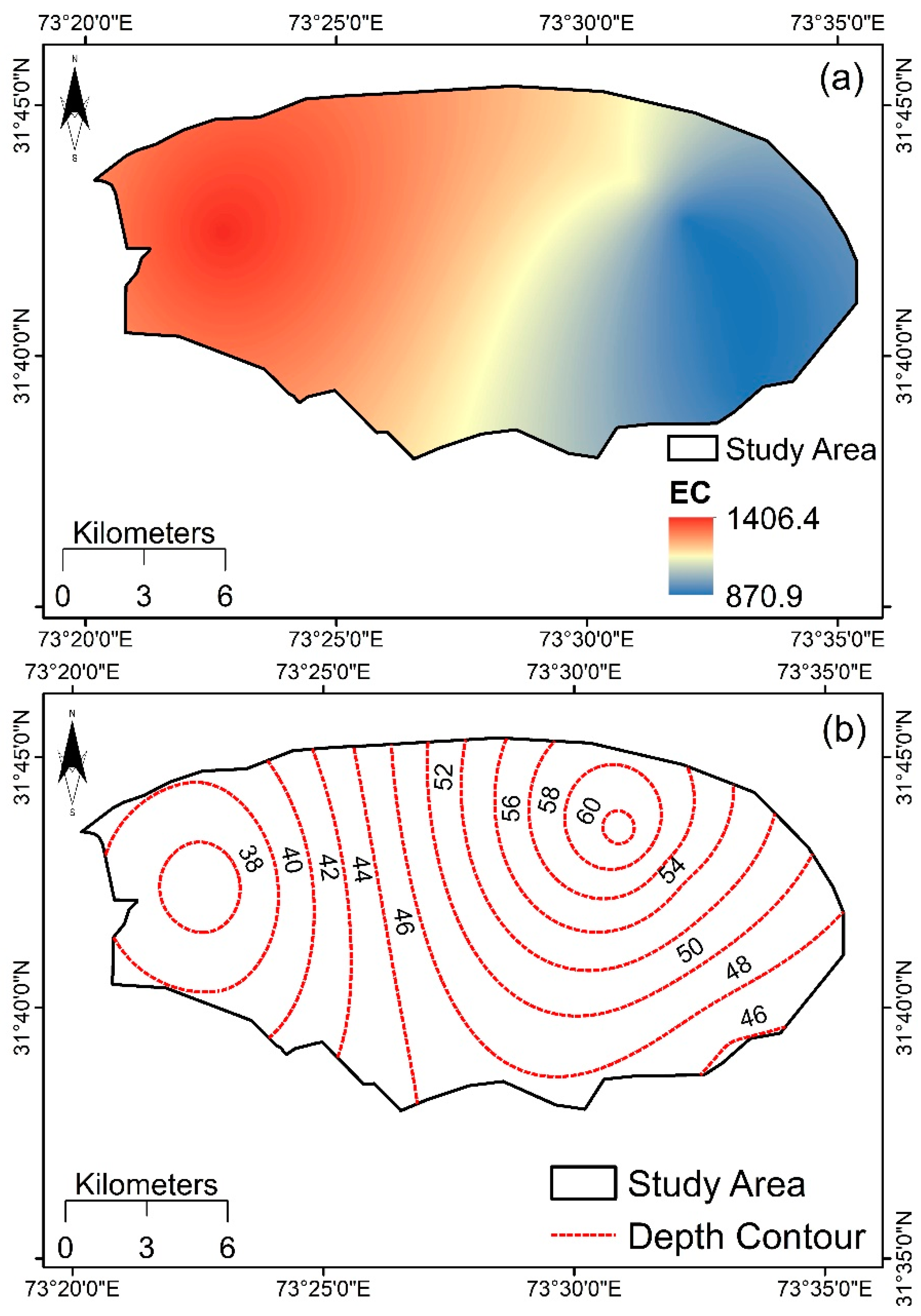
Figure 6a shows that the quality of groundwater is better in the NE area. The moderate values of the EC are observed in the rest of the area. The SE part contains the groundwater having the highest EC values. The NE area can be termed as a freshwater zone, while the rest of the area can be termed as brackish water as per guidelines by WHO 2008 [56]. In the entire study area, the EC values fall under the criteria given in Table 4. Almost 70 percent of the area has groundwater having a slight to moderate effect on crops. The groundwater from these areas can be utilized for a specific type of crops. The depth of tube wells from where water samples were taken is shown in Figure 4b.
3.6. Comparision of DRASTIC and EC
The validation was done by calculating the statistical relationship, covariance, and correlation matrix between DRASTIC results and EC. The higher correlation value indicates the accuracy of the results. The statistics of EC shows a minimum value of 870.21, maximum value of 1406, and a mean value of 1170.13. Standard deviation from the mean is 51.43. The statistics of DRASTIC shows a minimum value of 60.12, maximum value of 180, and a mean value of 97.72. Standard deviation from the mean is 11.44, as illustrated in Table 5. The covariance matrix between EC and DRASTIC is 945.51, displayed in Table 6. The correlation value between EC and DRASTIC is 0.712, as shown in Table 7.
4. Discussion
In this study, different approaches have been used for the incursion of groundwater vulnerability to contamination. The over-exploitation of human and natural resources of freshwater mainly contributes to contaminated water intrusion. The traditional methods for assessing fresh/saline water areas, including drilling, are costly, intrusive, cumbersome and time-consuming, and hardly easy to employ on a large scale [25]. This is the reason this study was carried out in the Safdarabad area of Punjab, Pakistan. This area is well known for its agriculture and for the production of the best quality rice in Pakistan [57]. The VES surveys have also been developed to evaluate the vulnerability of the soil to wastewater at low depths, which may percolate through the top clay cap from the drainage networks. The detailed investigation here includes resistivity tests integrated with the EC of groundwater samples, correlated and tested DRASTIC results, and resistivity results. Their relationship will help to assess the efficacy of the aquifer vulnerability index identified by the surface resistivity survey since it requires less data and less processing steps, thereby saving time and costs.
The results from the transverse resistance show the NE, North central, and NW areas as freshwater zones having the highest values of transverse resistance. However, the peak of the transverse resistance can be observed in the NE area, as in Figure 4a. The results from longitudinal resistivity show that good quality groundwater can be found in the NE and north central area since it shows high values of longitudinal resistivity at these points, as in Figure 4b. However, the rest of the area falls in the low longitudinal resistivity zone, making it fall under the category of saline water zone as per criteria by [58]. In the case of the EC results, the NE areas depict the lowest values indicating the freshwater zone, which does not have any effect on crops, according to Table 4. However the remaining area falls into the category of water having a slight to moderate effect on crops and can be termed as good for irrigation purposes according to the guidelines given by (WHO 2008) [56]. The groundwater in the NE area can also be utilized for drinking purposes after proper laboratory measurement according to criteria set by WHO 2008.
The final groundwater vulnerability integrated map of the DRASTIC model is illustrated in Figure 3, with the most vulnerable zone situated in the eastern region. Overall, the study area constitutes low vulnerability and covers 38% of the total area. The high vulnerability region is mainly located in the groundwater recharge areas, which means there is also high conductivity on the eastern side. This explains why the vulnerability index for this area is high. These maps can be used for regional irrigation planning or to determine the study area’s environmental vulnerability.
Shakoor [59] conducted a DRASTIC study in district Faisalabad. According to the findings, approximately one-third of the groundwater in the study region is at high risk of agricultural contamination, while nearly half of the aquifer is moderately vulnerable. High vulnerability zones are primarily found in high recharge zones, at lower depths, and in the sand medium. These same crucial factors are also dominated in our research area due to the close vicinity of Faisalabad with our study area geographically. Similarly, Kadkhodaie [60] found that the aquifer media and vadose zone have a significant influence on the Shabestar plain aquifer’s intrinsic vulnerability in NW Iran. Pacheco [61] mentioned that the one main factor for regulating inherent vulnerability within continental Portuguese territory is groundwater depth. Based on the above results and discussion, the DRASTIC method is adequate for vulnerability mapping in this area. The VES and EC methods, as well as the DRASTIC model, are used in our current analysis, giving it an advantage over other studies. The VES and EC identify the freshwater body and assess the variation in groundwater quality in the region in terms of salinity changes. It also monitors the interface of fresh and saltwater. The DRASTIC model provides an overview of possible vulnerable areas.
For the DRASTIC Model, the EC was used for correlation and to validate the DRASTIC results. The statistical relationship, covariance, and correlation matrix between DI and EC is illustrated in Table 5, Table 6 and Table 7. The covariance matrix shows that EC and DRASTIC are positively related and the correlation matrix between EC and DRASTIC shows positive correlation.
5. Conclusions
It is worth noting that our methodology suggests an approach to conducting a more comprehensive comparison and correlation between the VES, EC, and DRASTIC. The study was conducted using the DRASTIC model to evaluate the quality and the vulnerability of groundwater in Safdarabad by VES modelling. These two approaches allow us to update different parameter maps so that vulnerability zones can be classified for groundwater. In the DRASTIC vulnerability map, the results of the study are based on the standard DRASTIC model and distinguish between four groups of DRASTIC indexes: very high, medium, low, and very low contaminant susceptibility. The results from the VES and EC assessed the groundwater quality variation in terms of salinity changes in the area. Overall, the comparison of results reveals that the NE areas having fresh water are on a great verge of contamination due to the highest drastic index values at these points. However, the SE area has saline water and falls in the highest drastic index area. The rest of the area in NW and SW falls in the low drastic index area making it less vulnerable to contamination. However, the quality of groundwater in these areas, according to VES and EC results, falls in the brackish water zone. Overall, a comparison of the findings of the VES, EC, and DRASTIC shows that regions with decent groundwater quality are on the brink of contamination and need attention. The validation of DRASTIC and EC show a nearly positive correlation. There is a need for proper wastewater management policies to be implemented, and there is a direct need to install wastewater treatment plants in these areas.
Author Contributions
Conceptualization, S.H.I.A.S., I.U. and B.A.; methodology, A.T.; software, A.T.; validation, A.T. and J.Y.; formal analysis, S.H.I.A.S.; investigation, A.T. and F.M.; resources, S.H.I.A.S.; data curation, A.T., F.M. and S.H.I.A.S.; writing—original draft preparation, S.H.I.A.S. and A.T.; writing—review and editing, A.T., L.Z. and J.Y.; visualization, B.A., A.T., J.Y., L.Z. and F.M.; supervision, A.T. and L.Z.; project administration, L.Z. and A.T.; funding acquisition, L.Z. All authors have read and agreed to the published version of the manuscript.
Funding
This study was supported by National Natural Science Foundation of China (grant 41907192) and civil aerospace pre-research project (D040102).
Institutional Review Board Statement
Not applicable.
Informed Consent Statement
Not applicable.
Data Availability Statement
The data presented in this study are available on request from the first or corresponding authors.
Acknowledgments
We are thankful to the Chinese Government Scholarship. The authors are thankful to Muhammad Kashif Adeem, who provided guidance about the general hydrology of the study area.
Conflicts of Interest
The author states that there are no conflict of interest in printing this document. The writers have struggled with ethical issues in detail including plagiarism, informed consent, theft, evidence creation and/or falsification, simultaneous release and/or delivery, and duplication.
References
- (CGER) Commission on Geosciences. Ground Water Vulnerability Assessment: Predicting Relative Contamination Potential under Conditions of Uncertainty; The National Academies Press: Washington, DC, USA, 1993. [Google Scholar]
- Zaporozec, A. Groundwater Contamination Inventory: A Methodological Guide; IHP-IV Series on Groundwater No.2; UNESCO: Paris, France, 2002. [Google Scholar]
- Shirazi, S.M.; Imran, H.M.; Akib, S. GIS-based DRASTIC method for groundwater vulnerability assessment: A review. J. Risk Res. 2012, 15, 991–1011. [Google Scholar] [CrossRef]
- United Nations Development Programme Pakistan. Water Security in Pakistan: Issues and Challenges; UNDP: New York, NY, USA, 2016; Volume 3, pp. 1–34. [Google Scholar]
- Cosgrove, F.R.; Rijsberman, W.J. World Water Vision: Making Water Everybody’s Business; Routledge: London, UK, 2014. [Google Scholar]
- Davis, J. Private-sector participation in the water and sanitation sector. Annu. Rev. Environ. Resour. 2005, 30, 145–183. [Google Scholar] [CrossRef]
- Margat, J. Vulnerabilite des Mappes d’eau Souterraine a la Pollution; BRGM Publications: Orleans, France, 1968; Volume 68. [Google Scholar]
- SNIFFER (Scotland and Ireland Forum for Environmental Research). Development of a Groundwater Vulnerability Screening Methodology for the Water Framework Directive; Proj. Rep. Code WFD 28; SNIFFER: Edinburgh, UK, 2004. [Google Scholar]
- Neshat, A.; Pradhan, B.; Dadras, M. Groundwater vulnerability assessment using an improved DRASTIC method in GIS. Resour. Conserv. Recycl. 2014, 86, 74–86. [Google Scholar] [CrossRef]
- Sorichetta, A.; Masetti, M.; Ballabio, C.; Sterlacchini, S.; Beretta, G.P. Reliability of groundwater vulnerability maps obtained through statistical methods. J. Environ. Manag. 2011, 92, 1215–1224. [Google Scholar] [CrossRef]
- Milnes, E. Process-based groundwater salinisation risk assessment methodology: Application to the Akrotiri aquifer (Southern Cyprus). J. Hydrol. 2011, 399, 29–47. [Google Scholar] [CrossRef] [Green Version]
- Barbash, J.E.; Resek, E.A. Pesticides in Ground Water: Distribution, Trends, and Governing Factors; Ann Arbor Press: Chelsea, MI, USA, 1996. [Google Scholar]
- Jeannin, P.-Y.; Zwahlen, F.; Doerfliger, N. Water vulnerability assessment in karst environments: A new method of defining protection areas using a multi-attribute approach and GIS tools (EPIK method). Environ. Geol. 1999, 39, 165–176. [Google Scholar]
- Foster, S.S.D. Fundamental concepts in aquifer vulnerability, pollution risk and protection strategy. In Vulnerability of Soil and Groundwater to Pollutants; Duijvenbooden, W., Waegeningh, H.G., Eds.; Committee on Hydrological Research: The Hague, The Netherlands, 1987; pp. 69–86. [Google Scholar]
- Van Stempvoort, D.; Ewert, L.; Wassenaar, L. Aquifer vulnerability index: A gis—Compatible method for groundwater vulnerability mapping. Can. Water Resour. J. 1993, 18, 25–37. [Google Scholar] [CrossRef] [Green Version]
- Vrba, J.; Zaporozec, A. Guidebook on mapping groundwater vulnerability. Int. Contrib. Hydrogeol. 1994, 16, 131. [Google Scholar]
- Aller, L.; Bennett, T.; Lehr, J.H.; Petty, R.J.; Hackett, G. DRASTIC: A Standardized Method for Evaluating Ground Water Pollution Potential Using Hydrogeologic Settings; NWWA/EPA-600/2-87-035; U.S. Environmental Protection Agency: Washington, DC, USA, 1987. [Google Scholar]
- Maqsoom, A.; Aslam, B.; Khalil, U.; Ghorbanzadeh, O.; Ashraf, H.; Tufail, R.F.F.; Farooq, D.; Blaschke, T. A GIS-based DRASTIC Model and an Adjusted DRASTIC Model (DRASTICA) for Groundwater Susceptibility Assessment along the China–Pakistan Economic Corridor (CPEC) Route. ISPRS Int. J. Geo Inf. 2020, 9, 332. [Google Scholar] [CrossRef]
- Gad, M.; El-Hattab, M. Integration of water pollution indices and DRASTIC model for assessment of groundwater quality in El Fayoum depression, western desert, Egypt. J. Afr. Earth Sci. 2019, 158, 103554. [Google Scholar] [CrossRef]
- Hussain, Y.; Ullah, S.F.; Dilawar, A.; Akhter, G.; Martinez-Carvajal, H.; Roig, H.L. Assessment of the Pollution Potential of an Aquifer from Surface Contaminants in a Geographic Information System: A Case Study of Pakistan. Geo-Chicago 2016, 269, 623–632. [Google Scholar] [CrossRef]
- Gilani, S.R.; Mahmood, Z.; Hussain, M.; Baig, Y.; Abbas, Z. A Study of Drinking Water of Industrial Area of Sheikhupura with Special Concern to Arsenic, Manganese and Chromium. Pak. J. Eng. Appl. Sci. 2013, 13, 118–126. [Google Scholar]
- Aslam, B.; Ismail, S.; Ali, I. A GIS—based DRASTIC model for assessing aquifer susceptibility of Safdarabad Tehsil, Sheikhupura District, Punjab Province, Pakistan. Model. Earth Syst. Environ. 2020, 6, 995–1005. [Google Scholar] [CrossRef]
- Herckenrath, D.; Fiandaca, G.; Auken, E.; Bauer-Gottwein, P. Sequential and joint hydrogeophysical inversion using a field-scale groundwater model with ERT and TDEM data. Hydrol. Earth Syst. Sci. 2013, 17, 4043–4060. [Google Scholar] [CrossRef] [Green Version]
- Asfahani, J.; Zakhem, B.A. Geoelectrical and hydrochemical investigations for characterizing the salt water intrusion in the Khanasser valley, northern Syria. Acta Geophys. 2012, 61, 422–444. [Google Scholar] [CrossRef]
- Hasan, M.; Shang, Y.; Akhter, G.; Khan, M. Geophysical Investigation of Fresh-Saline Water Interface: A Case Study from South Punjab, Pakistan. Ground Water 2017, 55, 841–856. [Google Scholar] [CrossRef] [PubMed]
- Iyasele, J.U.; Idiata, D.J. Investigation of the Relationship between Electrical Conductivity and Total Dissolved Solids for Mono-Valent, Di-Valent and Tri-Valent Metal Compounds. Int. J. Eng. Res. Rev. 2015, 3, 40–48. [Google Scholar]
- Greenman, D.W.; Bennett, G.D.; Swarzenski, W.V. Ground-water hydrology of the punjab, west Pakistan, with emphasis on problems created by canal irrigation. J. Hydrol. 1967, 1, 312. [Google Scholar] [CrossRef]
- Nickson, R.T.; McArthur, J.M.; Shrestha, B.; Kyaw-Myint, T.O.; Lowry, D. Arsenic and other drinking water quality issues, Muzaffargarh District, Pakistan. Appl. Geochem. 2005, 20, 55–68. [Google Scholar] [CrossRef]
- Moustafa, M. Assessing perched aquifer vulnerability using modified DRASTIC: A case study of colliery waste in north-east England (UK). Hydrogeol. J. 2019, 27, 1837–1850. [Google Scholar] [CrossRef]
- Wu, X.; Li, B.; Ma, C. Assessment of groundwater vulnerability by applying the modified DRASTIC model in Beihai City, China. Environ. Sci. Pollut. Res. 2018, 25, 12713–12727. [Google Scholar] [CrossRef] [PubMed]
- Prasad, N.N. Assessment of groundwater resource in Nileshwar River basin. J. Appl. Hydrol. 2013, 16, 52–60. [Google Scholar]
- Hussien, B.M.; Fayyadh, A.S. Impact of intense exploitation on the groundwater balance and flow within Mullusi aquifer (arid zone, west Iraq). Arab. J. Geosci. 2013, 6, 2461–2482. [Google Scholar] [CrossRef]
- Hopkins, L.D. Methods for Generating Land Suitability Maps: A Comparative Evaluation. J. Am. Inst. Plann. 1977, 43, 386–400. [Google Scholar] [CrossRef]
- Beck, A.E. Physical Principles of Exploration Methods; Palgrave: London, UK, 1981. [Google Scholar] [CrossRef] [Green Version]
- Sikandar, P.; Bakhsh, A.; Arshad, M.; Rana, T. The use of vertical electrical sounding resistivity method for the location of low salinity groundwater for irrigation in Chaj and Rachna Doabs. Environ. Earth Sci. 2010, 60, 1113–1129. [Google Scholar] [CrossRef]
- Bobachev, C. IPI2Win: A Windows Software for an Automatic Interpretation of Resistivity Sounding Data; Moscow State University: Moscow, Russia, 2002; p. 320. [Google Scholar]
- Henriet, J.P. Direct Applications of the Dar Zarrouk Parameters in Ground Water SURVEYS*. Geophys. Prospect. 1976, 24, 344–353. [Google Scholar] [CrossRef]
- Utom, A.U.; Odoh, B.I.; Okoro, A.U. Estimation of Aquifer Transmissivity Using Dar Zarrouk Parameters Derived from Surface Resistivity Measurements: A Case History from Parts of Enugu Town (Nigeria). J. Water Resour. Prot. 2012, 4, 993–1000. [Google Scholar] [CrossRef] [Green Version]
- Maillet, R. The Fundamental Equations of Electrical Prospecting. Geophysics 1947, 12, 529–556. [Google Scholar] [CrossRef]
- Jakhrani, S.H.; Soni, H.L.; Shar, N.Z. Analysis of Total Dissolved Solids and Electrical Conductivity in Different Water Supply Schemes of Taluka Chachro, District Tharparkar. QUEST Res. J. 2019, 17, 1–5. [Google Scholar]
- Arnold, S.L.; Doran, J.W.; Schepers, J.; Wienhold, B.; Ginting, D.; Amos, B.; Gomes, S. Portable Probes to Measure Electrical Conductivity and Soil Quality in the Field. Commun. Soil Sci. Plant Anal. 2005, 36, 2271–2287. [Google Scholar] [CrossRef] [Green Version]
- Al Dahaan, S.A.M.; Al-Ansari, N.; Knutsson, S. Influence of Groundwater Hypothetical Salts on Electrical Conductivity Total Dissolved Solids. Engineering 2016, 8, 823–830. [Google Scholar] [CrossRef] [Green Version]
- Tariq, A.; Shu, H. CA-Markov Chain Analysis of Seasonal Land Surface Temperature and Land Use Land Cover Change Using Optical Multi-Temporal Satellite Data of Faisalabad, Pakistan. Remote Sens. 2020, 12, 3402. [Google Scholar] [CrossRef]
- Gupta, N. Groundwater Vulnerability Assessment using DRASTIC Method in Jabalpur District of Madhya Pradesh. Int. J. Recent Technol. Eng. 2014, 3, 36–43. [Google Scholar]
- Waqas, H.; Lu, L.; Tariq, A.; Li, Q.; Baqa, M.F.; Xing, J.; Sajjad, A. Flash Flood Susceptibility Assessment and Zonation Using an Integrating Analytic Hierarchy Process and Frequency Ratio Model for the Chitral District, Khyber Pakhtunkhwa, Pakistan. Water 2021, 13, 1650. [Google Scholar] [CrossRef]
- Sener, B.C.; Dergin, G.; Gursoy, B.; Kelesoglu, E.; Slih, I. Effects of irrigation temperature on heat control in vitro at different drilling depths. Clin. Oral Implant. Res. 2009, 20, 294–298. [Google Scholar] [CrossRef] [PubMed]
- Rahman, A. A GIS based DRASTIC model for assessing groundwater vulnerability in shallow aquifer in Aligarh, India. Appl. Geogr. 2008, 28, 32–53. [Google Scholar] [CrossRef]
- Lynch, S.D.; Reynders, A.G.; Schulze, R.E. Preparing input data for a national-scale groundwater vulnerability map of Southern Africa. Water SA 1994, 20, 239–246. [Google Scholar]
- Chandrashekhar, H.; Adiga, S.; Lakshminarayana, V.; Jagdeesha, C.; Nataraju, C. A case study using the model ‘DRASTIC’for assessment of groundwater pollution potential. In Proceedings of the ISRS National Symposium on Remote Sensing Applications for Natural Resources, Bangalore, India, 19–22 January 1999; pp. 19–21. [Google Scholar]
- Foster, S.S.D. Groundwater recharge and pollution vulnerability of British aquifers: A critical overview. Geol. Soc. Spec. Publ. 1998, 130, 7–22. [Google Scholar] [CrossRef]
- IRI. Groundwater Investigation for Sustainable Water Supply to FDA City Housing Scheme, Faisalabad; Research Report No IRR-Phy/577; Government of the Punjab, Irrigation Department, Irrigation Research Institute: Lahore, Pakistan, 2012. [Google Scholar]
- Khalid, P.; Sanaullah, M.; Sardar, M.J.; Iman, S. Estimating active storage of groundwater quality zones in alluvial deposits of Faisalabad area, Rechna Doab, Pakistan. Arab. J. Geosci. 2019, 12, 206. [Google Scholar] [CrossRef]
- Akhter, G.; Hasan, M. Determination of aquifer parameters using geoelectrical sounding and pumping test data in Khanewal District, Pakistan. Open Geosci. 2016, 8, 630–638. [Google Scholar] [CrossRef]
- Ayers, R.S.; Westcot, D.W. Water Quality for Agriculture; FAO Irrigation and Drainage Paper 29 Rev. 1; Food and Agricultural Organization: Rome, Italy, 1985. [Google Scholar]
- Kwiatkowski, J.; Pittman, J. Salinity Mapping for Resource Management within the M.D. of Provost, Alberta; Conservation and Development Branch Alberta Agriculture, Food and Rural Development: Edmonton, AB, Canada, 1997. [Google Scholar]
- WHO. Guidelines for Drinking-Water Quality, 3rd ed.; Recommendations Incorporating1ST and 2nd Addenda; World Health Organization: Geneva, Switzerland, 2008; Volume 1. [Google Scholar]
- Yasin, M.A.; Ashfaq, M.; Adil, S.A.; Bakhsh, K. Profit Efficiency of Organic Vs Conventional Wheat Production in Rice-Wheat Zone of Punjab, Pakistan. J. Agric. Res. 2014, 52, 439–452. [Google Scholar]
- Hasan, M.; Shang, Y.; Akhter, G.; Jin, W. Application of VES and ERT for delineation of fresh-saline interface in alluvial aquifers of Lower Bari Doab, Pakistan. J. Appl. Geophys. 2019, 164, 200–213. [Google Scholar] [CrossRef]
- Shakoor, A.; Khan, Z.M.; Farid, H.U.; Sultan, M.; Ahmad, I.; Ahmad, N.; Mahmood, M.H.; Ali, M.U. Delineation of regional groundwater vulnerability using DRASTIC model for agricultural application in Pakistan. Arab. J. Geosci. 2020, 13, 1–12. [Google Scholar] [CrossRef]
- Kadkhodaie, F.; Moghaddam, A.A.; Barzegar, R.; Gharekhani, M.; Kadkhodaie, A. Optimizing the DRASTIC vulnerability approach to overcome the subjectivity: A case study from Shabestar plain, Iran. Arab. J. Geosci. 2019, 12, 527. [Google Scholar] [CrossRef]
- FPacheco, A.L.; Martins, L.M.O.; Quininha, M.; Oliveira, A.S.; Fernandes, L.F.S. Modification to the DRASTIC framework to assess groundwater contaminant risk in rural mountainous catchments. J. Hydrol. 2018, 566, 175–191. [Google Scholar] [CrossRef]
Figure 1.
A location of the study area in Safdarabad Tehsil, Punjab.

Figure 2.
Seven thematic layers of the DRASTIC model: (a) depth to water table; (b) net recharge (c); aquifer media; (d) soil media; (e) slope; (f) vadose zone; and (g) hydraulic conductivity.
Figure 2.
Seven thematic layers of the DRASTIC model: (a) depth to water table; (b) net recharge (c); aquifer media; (d) soil media; (e) slope; (f) vadose zone; and (g) hydraulic conductivity.

Figure 3.
Drastic vulnerability map of the area.

Figure 4.
Geoelectrical Parameters: (a) transverse resistance and (b) longitudinal resistance.

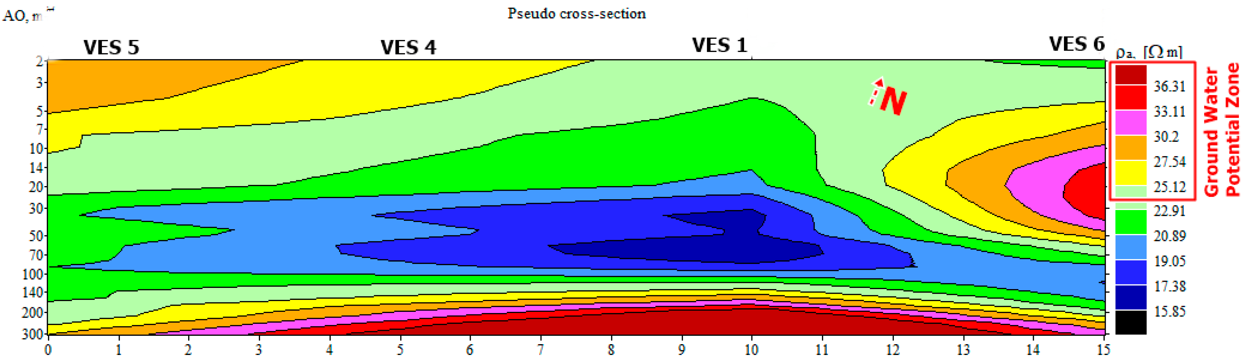
Figure 5.
Pseudo Resistivity Cross section for A to A’ from Figure 4. The area in cross-section A to A’ shows high resistivity zones even in the shallow depths. After approximately 110 m, the resistivity is increasing, indicating a good groundwater potential zone having better quality water. The reason for high resistivity at these points corresponds to the presence of a recharge source which is a canal in this case. The areas having recharge resources near to them will have not only shallow water tables but also have good quality water [27].

Figure 6.
(a) Map for the EC variation in the area; (b) depth of the tube wells from where groundwater sample was taken.
Figure 6.
(a) Map for the EC variation in the area; (b) depth of the tube wells from where groundwater sample was taken.


Table 1.
All of the parameters’ data sources are listed in this table.
| S.No | Parameter | Source |
|---|---|---|
| 1 | Depth to water table | Pakistan Council of Research in Water Resources (PCRWR) |
| 2 | Net recharge | Rainfall Dataset from Pakistan Meteorological Department (PCRWR) |
| 3 | Aquifer media | Soil Survey of Pakistan and Pakistan Council of Research in Water Resources (PCRWR) |
| 4 | Soil media | Soil Survey of Pakistan and Pakistan Council of Research in Water Resources (PCRWR) |
| 5 | Topography | SRTM DEM, Acquired from (https://earthexplorer.usgs.gov/, accessed on 26 December 2020)) |
| 6 | Impact of vadose zone | Soil Survey of Pakistan and Pakistan Council of Research in Water Resources (PCRWR) |
| 7 | Hydraulic conductivity | Soil Survey of Pakistan and Pakistan Council of Research in Water Resources (PCRWR) |
Table 2.
Weights and ranges allocated to various factors used in the contamination vulnerability assessment [45,46].
| Parameter | Range | Rating | Weight |
|---|---|---|---|
| Depth to water table (m) | <40 | 9 | 5 |
| 40–60 | 7 | ||
| 60–80 | 5 | ||
| 80–100 | 3 | ||
| >100 | 1 | ||
| Net recharge (mm) | >80 | 9 | 4 |
| 60–80 | 7 | ||
| 40–60 | 5 | ||
| <40 | 3 | ||
| Aquifer media | Sand | 8 | 3 |
| Soil media | Sandy loam | 8 | 2 |
| Loamy | 7 | ||
| Clayey soil | 5 | ||
| Salt affected soil | 4 | ||
| Topography | <5 | 9 | 1 |
| 5–10 | 8 | ||
| 10–20 | 6 | ||
| 20–40 | 4 | ||
| >40 | 2 | ||
| Impact of vadose zone | Sand | 7 | 5 |
| Hydraulic conductivity | >200 | 9 | 3 |
| 150–200 | 8 | ||
| 100–150 | 6 | ||
| <100 | 4 |
| S.No | Resistivity Zone | Apparent Resistivity (Ωm) | Interpretation Lithology | Ground Water Potential Zone |
|---|---|---|---|---|
| 1 | Zone above water | Haphazard | Surface Materials | Low Potential Zone |
| 2 | Medium Resistivity Zone | >25 Ωm | Medium to coarse sand or Kankers Intermixed thin Silty Clay layers | High potential Zone |
| 3 | Low Resistivity Zone | 15–25 Ωm | Fine to medium sand Intermixed with thin Silty layers | Medium Potential Zone |
| 4 | Very Low Resistivity Zone | <15 Ωm | The admixture of fine sand, clay, and silt | Low Potential Zone |
Table 4.
Deduced from guidelines for interpretation of water quality for irrigation, modified from [54,55].
| Potential Irrigation Problem | Unit | Degree of Restriction | ||
|---|---|---|---|---|
| None | Slight to Moderate | Severe | ||
| EC | μS/cm | <1000 | 1000 to 2500 | >3000 |
| TDS | mg/L | <700 | 700–2000 | >2000 |
Table 5.
Statistics of individual layers.
| Layer | Min | Max | Mean | STD |
|---|---|---|---|---|
| EC | 870.21 | 1406 | 1170.13 | 51.43 |
| DRASTIC | 60.12 | 180 | 97.72 | 11.44 |
Table 6.
Covariance matrix between EC and DRASTIC.
| Layer | EC | DRASTIC |
|---|---|---|
| EC | 1753.54 | |
| DRASTIC | 945.51 | 20,471.65 |
Table 7.
Correlation matrix between EC and DRASTIC.
| Layer | EC | DRASTIC |
|---|---|---|
| EC | 1 | |
| DRASTIC | 0.712 | 1 |
Publisher’s Note: MDPI stays neutral with regard to jurisdictional claims in published maps and institutional affiliations. |
© 2021 by the authors. Licensee MDPI, Basel, Switzerland. This article is an open access article distributed under the terms and conditions of the Creative Commons Attribution (CC BY) license (https://creativecommons.org/licenses/by/4.0/).
Share and Cite
MDPI and ACS Style
Shah, S.H.I.A.; Yan, J.; Ullah, I.; Aslam, B.; Tariq, A.; Zhang, L.; Mumtaz, F. Classification of Aquifer Vulnerability by Using the DRASTIC Index and Geo-Electrical Techniques. Water 2021, 13, 2144. https://doi.org/10.3390/w13162144
AMA Style
Shah SHIA, Yan J, Ullah I, Aslam B, Tariq A, Zhang L, Mumtaz F. Classification of Aquifer Vulnerability by Using the DRASTIC Index and Geo-Electrical Techniques. Water. 2021; 13(16):2144. https://doi.org/10.3390/w13162144
Chicago/Turabian StyleShah, Syed Hassan Iqbal Ahmad, Jianguo Yan, Israr Ullah, Bilal Aslam, Aqil Tariq, Lili Zhang, and Faisal Mumtaz. 2021. "Classification of Aquifer Vulnerability by Using the DRASTIC Index and Geo-Electrical Techniques" Water 13, no. 16: 2144. https://doi.org/10.3390/w13162144
Note that from the first issue of 2016, this journal uses article numbers instead of page numbers. See further details here.