Q-Learnheuristics: Towards Data-Driven Balanced Metaheuristics

Abstract

One of the central issues that must be resolved for a metaheuristic optimization process to work well is the dilemma of the balance between exploration and exploitation. The metaheuristics (MH) that achieved this balance can be called balanced MH, where a Q-Learning (QL) integration framework was proposed for the selection of metaheuristic operators conducive to this balance, particularly the selection of binarization schemes when a continuous metaheuristic solves binary combinatorial problems. In this work the use of this framework is extended to other recent metaheuristics, demonstrating that the integration of QL in the selection of operators improves the exploration-exploitation balance. Specifically, the Whale Optimization Algorithm and the Sine-Cosine Algorithm are tested by solving the Set Covering Problem, showing statistical improvements in this balance and in the quality of the solutions.

1. Introduction

In approximate methods, the guarantee of finding global optimum solutions is sacrificed due to the computational complexity of hard optimization problems. Approximate algorithms can be classified as specific heuristics and MH. Heuristics are techniques specifically designed to solve a particular problem. On the contrary, MH are defined as upper-level general methodologies (templates), which can be used as guiding strategies for the design of underlying heuristics for solving a problem [1]. Then, MH extends basic heuristic methods by including them in an iterative framework, augmenting their exploration and exploitation capabilities. Notice that exploration is the process of visiting new regions of a search space (solutions), whereas exploitation is the process of visiting those regions within the neighborhood of previously visited solutions. Thus, MH needs to establish a good ratio between exploration and exploitation to be successful. That means that designing and applying good MH is to make a proper trade-off between these two “forces” [2,3]. Unfortunately, the proper handling of this trade-off is an open question in the literature [4,5,6,7,8,9]. A comprehensive review about MH can be found in [1,10].

Optimization problems can be classified depending on the domain of the decision variables in discrete and continuous problems. In recent years, discrete optimization problems have become more and more frequent in the industry with problems as Set Covering Problem (SCP) [11,12], Knapsack Problem [13], Software Project Scheduling Problem [14,15] and Feature Selection [16]. The No-Free-Lunch Theorem (NFLT) [17] tells us that there is no universal optimization algorithm for all existing optimization problems. This means that, despite the existence of algorithms designed to solve discrete problems, none of them are good for all combinatorial optimization problems and there will always be a better one for a specific problem. This best algorithm can be one designed for discrete problems as well as an algorithm designed for continuous problems adapted to discrete problems. However, there are many MH (most of them are swarm intelligence) designed to work in the continuous domain, meaning that binarization techniques are required [18]. Among the most commonly used binarization operators, two-step techniques are the most common [18] and its performance has been improved by the use of ml-based techniques [13,19].

Several variations of MH are proposed in the literature to improve MH algorithms. Among the most relevant trends, hybrid MH represent a class of algorithms that combine MH with other applicable algorithms. The resulting algorithms take advantage of the strengths of algorithms composing the hybridization, finding better results while keeping complexity low. According to the taxonomy defined in [1] for hybrid MH, MH are usually combined with MH with exact mathematical programming algorithms (resulting in matheuristics [20]), with simulation (resulting in simheuristics [21]) and with machine learning (ML) (resulting in learnheuristics [22,23,24]). This work focuses on proposing a learnheuristic.

Focusing on ML, these techniques have become popular in recent years with many applications, from industrial to everyday applications [25,26]. Usually, ML techniques are divided in supervised, unsupervised, semi-supervised and Reinforcement Learning. Supervised techniques learn from labeled data to infer future samples in the form of classification or regression [27]. Unsupervised techniques consider unlabeled data to find clusters or patterns with usual algorithms as k-means [28], dbscan [29] or BIRCH [30]. Semi-supervised techniques share features of supervised and unsupervised learning, resulting in a hybrid approach in which labeled data are managed in a supervised manner while unlabeled data are managed in an unsupervised manner [31]. Reinforcement Learning techniques are based on the notion of cumulative reward, where the system received a positive or negative reward after each decision, adjusting the behavior of the system according to this feedback. Thus, instead of learning from labeled data, as supervised techniques, the system learns from the experience of making decisions [32].

Based on the existing difficulties in applying binarization techniques in MH algorithms designed for solving continuous problems, the main contribution in this paper consists in a novel binarization scheme powered by the QL algorithm, which is a Reinforcement-Learning technique. The authors apply this binarization scheme in conjunction with two MH to solve the SCP, resulting in two hybrid MH. As a result, the authors verified that the hybrid approach including the novel binarization scheme outperforms the regular MH with a usual fixed binarization approach from the literature.

The reminder of this paper is organized as follows. Section 2 presents the related work. In Section 3, the classical binarizarion techniques are described. Section 4 describes the QL based binarization scheme proposed in this paper. Section 5 explains the two implemented MH. Section 6 presents SCP. Section 7 details the statistical methodology and the experimental results. Finally, Section 8 concludes the work with some final remarks.

2. Related Work

This section discusses related work along two lines. First, works in which metaheuristics are improved by applying ML techniques and, second, works in which Q-Learning is applied together with MH, resulting in hybrid MH.

2.1. Metaheuristics Enhanced by Machine Learning

Regarding ML techniques supporting MH, the work of García et al. [19] reviewed two lines of research. The first one consists in the integration of ML as a replacement for an operator (e.g., population management, solution initialization, local search, disturbance of solutions and parameter tuning, among others). The second one consists in the use of ML as a selection tool for a set of MH, choosing the most appropriate for solving an specific instance of a problem.

Regarding the first line, the authors may cite the work of Veček et al. [33], where they performed a parameter tuning for the chess rating system problem. In the work of Ries et al. [34], a similar implementation was performed but using fuzzy logic and Decision Trees. Deng et al. [35] proposed a clustering-based initial solution generation for the Traveling Salesman Problem. Within this line, the binarization operator was also of considerable interest. Some examples are observed in [13] by solving the Multidimensional Knapsack Problem by unsupervised learning techniques, in [36] by using the concept of percentile and in [37] where they implemented the framework of Apache Spark for large combinatorial problems.

When considering ML as a selection tool to obtain a MH among a set of these, this task is divided into three groups. The first one is the algorithm selection that chooses among a set of techniques and characteristics of each problem in order to obtain better performance for a set of similar instances [38]. The second one is the hyperheuristic strategies, which aims at automating the design of the MH to address a set of problems [39]. The third group is composed of cooperative strategies, which combine algorithms in a sequential and parallel manner to improve robustness, sharing a part of the solution or its totality [40].

Reinforcement Learning is often used for the intelligent selection of operators [41]. An example of this is the work of Zhang et al. [42] where they proposed an adaptive evolutionary programming algorithm. For each individual, an optimal mutation operator was selected based on immediate performance.

2.2. Metaheuristics Enhanced by Q-Learning

Reviewing the literature, it is possible to find various implementations of QL supporting MH to solve a wide range of problems. Among the first works are those made by Gambardella and Dorigo, where they incorporate QL replacing pheromone behavior in Ant Colony Optimization [43] to solve Travelling Salesman Problem [44] and its asymmetric version. In [45], QL is used as an heuristic selector inside an hyperheuristic scheme to solve the Cutting Stock Problem. The same strategy is used in [46,47] in order to solve the cross-domain heuristic search challenge [48] and Stochastic mixed-model assembly line sequencing problem. In [42,49], a hybridization is proposed where QL is an intelligent selector of mutation operators in Genetic Algorithms. In [50], QL and SARSA are implemented for League Championship Algorithm to strengthen the search power of each individual in the algorithm to extract better stock trading rules for various types of trading conditions. In [51,52], parameters of the Firefly Algorithm [53] and a version Sine Cosine Algorithm combined with Cuckoo Search are dynamically controlled to improve the search and to avoid falling into local optima. There are also several implementations in the literature where QL supports MH, such as Particle Swarm Optimization [54,55], Cuckoo Search [56], Bat Algorithm [57] and Meta-RaPS [58].

Summarizing what has been found in the literature, two models of conceptual interaction between QL and a MH are shown and these two major interest groups are: (1) how QL can support within the MH; and (2) how QL can support from outside the MH (with a hyperheuristic approach).

The interaction model shows that QL can support learning from the behavior of operators associated with the MH for the problem in the search of solutions, i.e., it is an additional element to the layer of the MH.

On the other hand, QL can be a component of a higher-level layer called Hyperheuristics (HH), which is given back to operators at a lower level with each iteration of the MH addressing the problem. The operators from the lower level problem form part of the problem to be solved at the top layer where any MH learning from QL can take place.

The literature review shows the contribution of ML works to improve the performance of metaheuristics as well as the contribution of metaheuristics to improve the performance of ML. However, in an essential topic in the behavior of a MH, such as the exploration-exploitation balance, there is an area of research that is interesting to work on in order to find better solutions that are applicable to the industry.

3. Continuous Metaheuristics Working in Binary Domains

The binary techniques for continuous MH consist of transferring the values of continuous domain of the MH to a binary domain, this is conducted to preserve the quality movements that possess continuous MH and, thus, generate quality binary solutions.

Although there are MH that work in binary domains without the need to incorporate a binary scheme, the continuous MH together with a binary scheme have presented great performance in diverse combinatorial NP-Hard problems for which they have called the interest of the scientific community. Some examples include Particle Swarm Optimization [59], Binary Salp Sawrm Algorithm [60], Binary Dragonfly [61] and Binary Magnetic Optimization Algorithm [62], among others [63,64,65,66].

Among the binary schemes, two large groups can be defined: First, the operators that do not alter the operation of the other elements of the MH where the two-step techniques stand out, as they are the most used previously [18] and the Angle Modulation technique [67]. The second group consists of the methods that alter the normal functioning of MH, which are Quantum Binary [68] and Set-Based Approaches in addition to the techniques based on clustering [13,19].

3.1. Two-Step Binarization Scheme

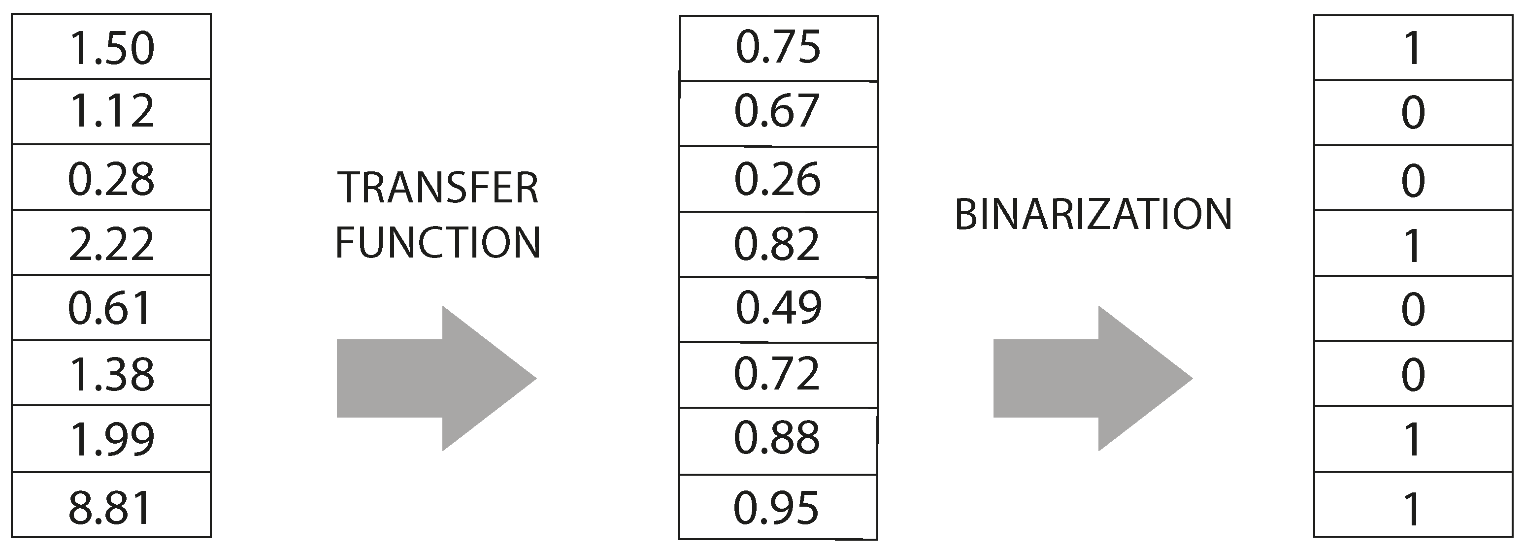
Two-step binary schemes are of great relevance for various types of problems [69]. This binarization scheme is composed by two steps, the first one is the transfer function, which transfers the values generated by the continuous MH to a continuous interval between 0 and 1, while the second step is the binarization, which consists in transferring the real number in a binary value. This is best exemplified in Figure 1.

3.1.1. Transfer Functions

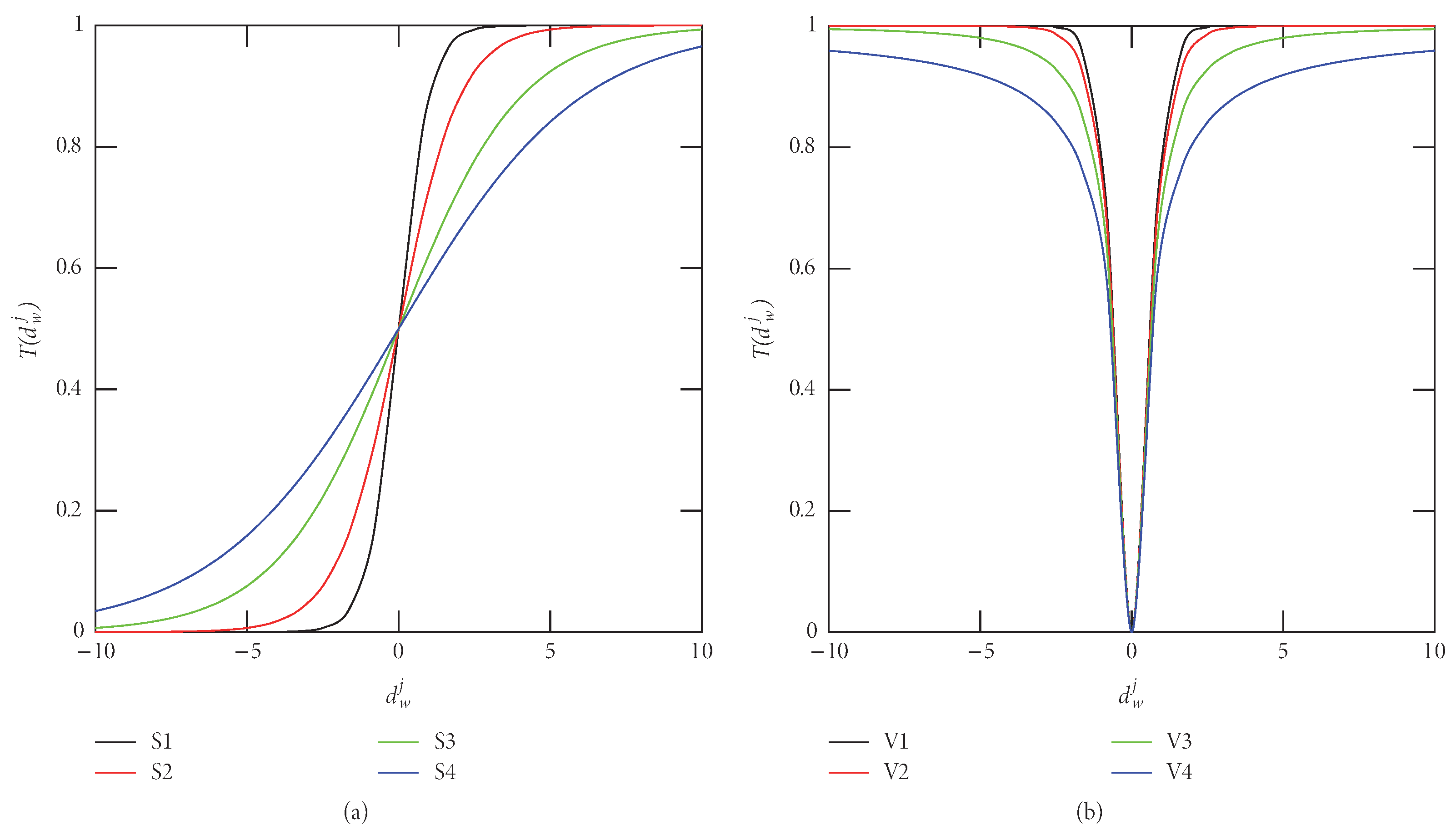
Transfer functions were introduced by Kennedy et al. in 1997 [70]. Having as main advantage the delivery of a probability between 0 and 1 at a low computational cost. There are two types of functions, the S-Shaped [63] and the V-Shaped [71] where each has four variations presented for both the S-Shape and for the V-Shape. The variations for the S-Shape functions, $T_{S_i}\left(d_w^j\right)$ for $i\in \{1,2,3,4\}$ are defined as follows:

$$T_{S_1}\left(d_w^j\right)=\frac{1}{1+e^{-2d_w^j}},$$

(1)

$$T_{S_2}\left(d_w^j\right)=\frac{1}{1+e^{-d_w^j}},$$

(2)

$$T_{S_3}\left(d_w^j\right)=\frac{1}{1+e^{\frac{-d_w^j}{2}}},$$

(3)

and

$$T_{S_4}\left(d_w^j\right)=\frac{1}{1+e^{\frac{-d_w^j}{3}}},$$

(4)

where $d_w^j$ denotes the discrete value in the individual $w\in \{1,2,\cdots ,n\}$ in dimension $j\in \{1,2,\cdots ,l\}$ and n and l are the number of individuals and dimensions, respectively. The variations for the V-Shape functions, $T_{V_i}\left(d_w^j\right)$ for $i=1,2,3,4$, are defined as follows:

$$T_{V_1}\left(d_w^j\right)=\left|erf\left(\frac{\sqrt{\pi }}{2}{d}_w^j\right)\right|,$$

(5)

$$T_{V_2}\left(d_w^j\right)=\left|tanh\left(d_w^j\right)\right|,$$

(6)

$$T_{V_3}\left(d_w^j\right)=\left|\frac{d_w^j}{\sqrt{1+{\left(d_w^j\right)}^2}}\right|,$$

(7)

and

$$T_{V_4}\left(d_w^j\right)=\left|\frac{2}{\pi }arctan\left(\frac{\pi }{2}{d}_w^j\right)\right|.$$

(8)

The results of plotting the tuples $(d_w^j,T_{S_i}\left(d_w^j\right))$ and $(d_w^j,T_{V_i}\left(d_w^j\right))$ for $i\in \{1,2,3,4\}$ are shown in Figure 2.

3.1.2. Binarization

The second step is binarization, which has the function of discretizing the probability obtained from the transfer function $T\left(d_w^j\right)$ calculated according to Section 3.1.1 by delivering a binary value.

For this step, there are different techniques in the literature such as Standard, Complement, Static Probability, Elitist and Elitist Roulette. The values for the binarization obtained by using different methods are defined as follows.

Let $X_{new,sd}^j$ be the binarization value obtained by using the Standard method. Then, $X_{new,sd}^j$ is defined as the following:

$$X_{new,sd}^j=\left\{\begin{array}{cc}1\hfill & \mathrm{if} rand\le T\left(d_w^j\right)\hfill \\ 0\hfill & \mathrm{otherwise}\hfill \end{array}\right.,$$

(9)

where $rand$, for $0\le rand\le 1$, is a random value generated following a uniform distribution $U(0,1)$, $T\left(d_w^j\right)$ denotes the discrete value in the individual $w\in \{1,2,\cdots ,n\}$ in dimension $j\in \{1,2,\cdots ,l\}$ and n and l are the number of individuals and dimensions, respectively.

Let $X_{new,c}^j$ be the binarization value obtained by using the Complement method. Then, $X_{new,c}^j$ is defined as the following:

$$X_{new,c}^j=\left\{\begin{array}{cc}Complement\left(X_w^j\right)\hfill & \mathrm{if} rand\le T\left(d_w^j\right)\hfill \\ 0\hfill & \mathrm{otherwise}\hfill \end{array}\right.,$$

(10)

where $Complement\left(X_w^j\right)$ denotes the complementary binary value of $X_w^j$ in the individual w for dimension j, i.e., if the value of $X_w^j$ is 0, the complement corresponds to 1.

Let $X_{new,sp}^j$ be the binarization value obtained by using the Static Probability method. Then, $X_{new,sp}^j$ is defined as the following:

$$X_{new,sp}^j=\left\{\begin{array}{cc}0\hfill & \mathrm{if} T\left(d_w^j\right)\le \alpha \hfill \\ X_w^j\hfill & \mathrm{if} \alpha <T\left(d_w^j\right)\le \frac{1}{2}(1+\alpha )\hfill \\ 1\hfill & \mathrm{if} T\left(d_w^j\right)>\frac{1}{2}(1+\alpha )\hfill \end{array}\right.,$$

(11)

where $X_w^j$ denotes the value of the dimension $j\in \{1,2,\cdots ,l\}$ in the individual $w\in \{1,2,\cdots ,n\}$, l and n are the number of dimensions and individuals, respectively, and $\alpha$ corresponds to a parameter determined by the user.

Let $X_{new,e}^j$ be the binarization value obtained by using the Elitist method. Then, $X_{new,e}^j$ is defined as the following:

$$X_{new,e}^j=\left\{\begin{array}{cc}{X}_{Best}^j\hfill & \mathrm{if} rand<T\left(d_w^j\right)\hfill \\ 0\hfill & \mathrm{otherwise}\hfill \end{array}\right.,$$

(12)

where $X_{Best}^j$ denotes the value of the dimension j in the individual $best$, which has obtained the best fitness so far, and l and n are the number of dimensions and individuals, respectively.

Let $X_{new,er}^j$ be the binarization value obtained by using the Elitist Roulette method [72]. Then, $X_{new,er}^j$ is defined as follows.

$$X_{new,er}^j=\left\{\begin{array}{cc}P[X_{new,er}^j={\zeta }_j]={\displaystyle \frac{f\left({\zeta }_j\right)}{{\sum }_{\delta \in Q_g}f\left(\delta \right)}}\hfill & \mathrm{if} rand<T\left(d_w^j\right)\hfill \\ P[X_{new,er}^j=0]=1\hfill & \mathrm{otherwise}\hfill \end{array}\right.,$$

(13)

4. Binarization Scheme Selector Proposal

Nowadays, combinatorial problems in the binary domain are becoming increasingly complex and frequent in the industry. Solving them in reasonable a reasonable time period with high quality solutions is a priority for both academia and the industry.

This work proposes an intelligent selector of binarization schemes where the existing binarization methods in the literature are integrated to control the exploration and exploitation balance, thus, avoiding local optimizations. This is because several authors [5,8,73,74,75] propose that for a metaheuristic to work well, it must have a good balance between exploration and exploitation. Exploration or diversification consists of visiting unexplored regions of the search space to ensure that the search is performed in biased regions [1]. In contrast, exploitation or intensification and promising regions with good solutions are further explored in hopes of finding better solutions [1].

This new binarization strategy is inspired by the behavior of hyperheuristics and techniques that have performed well for various types of problems [39,76,77,78]. This method consists in using an intelligent operator to determine which type of binarization is most appropriate at the iteration level, i.e., based on the information of the problem and the results obtained in previous iterations, the binarization scheme that is most likely to obtain the best quality results can be used.

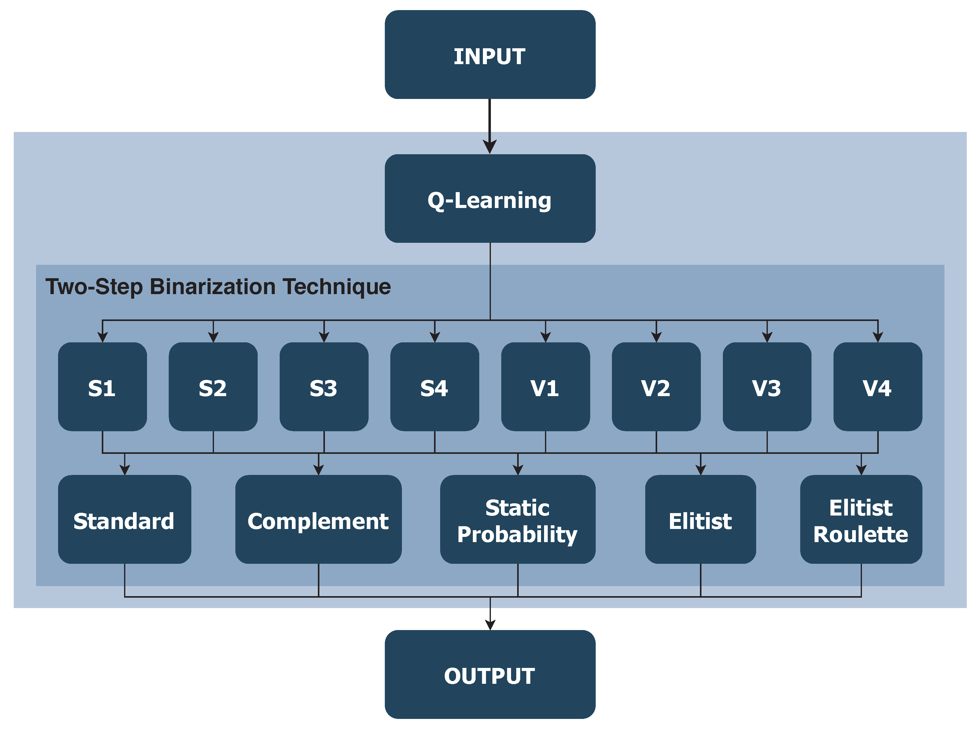
4.1. Q-Learning as a Smart Operator

In the present work, QL is implemented as the intelligent operator of the proposal, which chooses the two-step binarization technique to be used according to a reward system, with which it learns in a deterministic way. The structure of the implemented proposal is exemplified in Figure 3.

4.2. Q-Learning

Within Reinforcement Learning (RL) techniques there are Time Difference (TD) algorithms, which are characterized by exploring the environment and by using this information to update the current state [32]. The TD algorithms show the difference between the current estimation of the value of a state, the discounted value of the next state and the reward. It focuses on state-to-state transitions and learned values of states.

Prominent among the TD algorithms is QL [79], which provides agents with the ability to learn to act in the best way through the consequences of their actions taken. There are different “states” and different possible “actions” where the working “environment” is the current state in which the agent is in and must select and execute an action which affects the “environment” by changing its state. Actions are punished or rewarded by “rewards”, which are judged by the consequence obtained by applying an action in a particular state. Rewards are delayed, allowing the agent to learn from the system. In order to solve the problem, the agent tries to learn the best course of actions that will maximize the accumulated reward. The learning process lies in a set of episodes, where in each episode the agent selects and executes an action in a particular state. For the new episode, the agent’s learning is given by Equation (14):

$$Q_{new}(s_t,a_t)=(1-\alpha )·Q_{old}(s_t,a_t)+\alpha ·[r_t+\gamma ·maxQ(s_{t+1},a_{t+1})]$$

(14)

where $Q_{new}(s_t,a_t)$ is called Q-value and represents the cumulative quality or reward of the action taken $a_t$ in state $s_t$ at time t; $r_t$ is the reward or punishment received when action $a_t$ is taken in state $s_t$ at time t; $Q_{old}$ is the Q-value for the previous iteration for action $a_t$ in state $s_t$; $maxQ(s_{t+1},a_{t+1})$ is the maximum Q-value of the action for the next state, i.e., the best action the agent can take in the next state; $\alpha$ is the learning factor for which its value must be $0\le \alpha \le 1$; and $\gamma$ is the discount factor for which its value must be $0\le \gamma \le 1$. If $\alpha$ is close to 0, the historical information learned becomes more relevant, whereas if $\alpha$ is close to 1 the information received immediately becomes more relevant. If $\gamma$ equals 0, only the immediate reward is taken into account, while, as it approaches 1, the future reward receives greater emphasis relative to the immediate reward. The procedure of this algorithm is reflected in Algorithm 1.

Algorithm 1 Q-Learning Algorithm.

1: Initialize $Q_{values}$, $\alpha$, $\gamma$ 2: whilet < Maximum number of iterations do 3:     Choose $a_t$ base on $Q_{values}$ 4:     Execute action $a_t$ and get immediate reward or punishment $r_t$ 5:     Observe the next state $s_{t+1}$ 6:     $Q_{new}(s_t,a_t)=(1-\alpha )·Q_{old}·(s_t,a_t)+\alpha ·[r_t+\gamma ·maxQ(s_{t+1},a_{t+1})]$ 7:     $t\leftarrow t_{+1}$ 8: end while 9: Return $Q_{new}(s_t,a_t)$

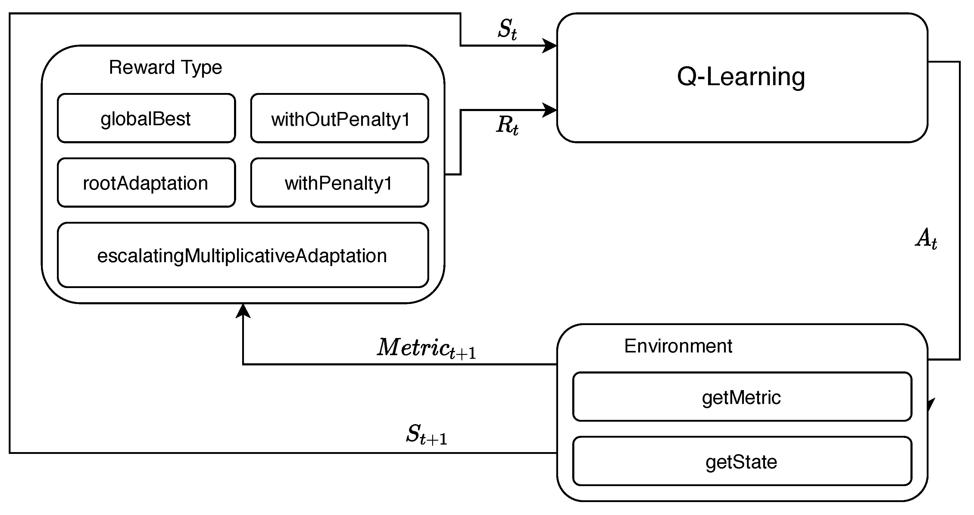
4.3. Rewards

The reward in the RL algorithm is fundamental for a correct performance of these same algorithms; that is why, in the literature, there are several methods to calculate the rewards. The type of reward from the chosen metrics determine the value $R_t$ for the general QL equation, as detailed in Figure 4.

For the implementation of this work, five forms of rewards were used where two of them are among the simplest in the literature. The first is the one used in [46,54], where it is increased by a fixed value for the action that generated an improvement in the overall fitness of the problem and a decrease in the same fixed value if no improvement was generated. This fixed value is detailed in Equation (15). The second type of reward is a variation of the previous one used in the Q-table, where there is no penalty on the Q-table values, as presented in Equation (16). The last three rewards are collected by Nareyek in [80], which are detailed in Equations (17)–(19), respectively:

$$withPenalty1=\left\{\begin{array}{cc}+1\hfill & \mathrm{if} \mathrm{there} \mathrm{is} \mathrm{a} \mathrm{fitness} \mathrm{improvement}\hfill \\ -1\hfill & \mathrm{otherwise}\hfill \end{array}\right.,$$

(15)

$$withOutPentalty1=\left\{\begin{array}{cc}+1\hfill & \mathrm{if} \mathrm{there} \mathrm{is} \mathrm{a} \mathrm{fitness} \mathrm{improvement}\hfill \\ 0\hfill & \mathrm{otherwise}\hfill \end{array}\right.,$$

(16)

$$globalBest=\left\{\begin{array}{cc}{\displaystyle \frac{W}{BestFitness}}\hfill & \mathrm{if} \mathrm{there} \mathrm{is} \mathrm{a} \mathrm{fitness} \mathrm{improvement}\hfill \\ 0\hfill & \mathrm{otherwise}\hfill \end{array}\right.,$$

(17)

$$rootAdaptation=\left\{\begin{array}{cc}\sqrt{BestFitness}\hfill & \mathrm{if} \mathrm{there} \mathrm{is} \mathrm{a} \mathrm{fitness} \mathrm{improvement}\hfill \\ 0\hfill & \mathrm{otherwise}\hfill \end{array}\right.,$$

(18)

and

$$escalatingMultiplicativeAdaptation=\left\{\begin{array}{cc}W·BestFitness\hfill & \mathrm{if} \mathrm{there} \mathrm{is} \mathrm{a} \mathrm{fitness} \mathrm{improvement}\hfill \\ 0\hfill & \mathrm{otherwise}\hfill \end{array}\right.,$$

(19)

where W and $BestFitness$ are defined as a constant of value 10 and the best fitness found so far, respectively.

4.4. Actions $A_t$

As mentioned above, the main objective of Q-Learning is to find an optimal policy within a set of actions. Therefore, it is important to define which actions the agent will take during its learning process. In the present work, the actions taken by the agents are the combinations between the transfer functions and the binarization functions extracted from the Two-Step Technique. Thus, we obtain 40 possible actions to be selected in the learning process.

4.5. Obtaining Metrics (getMetric)

The reward or punishment is judged by the consequence obtained by the performance of the action. Therefore, it is important to define what the comparison metrics will be to discriminate the consequence. In the present work, the comparison metric is the fitness obtained in each iteration of the optimization process and it is compared with the best fitness obtained. If fitness improves, action is rewarded, while if fitness worsens, action is punished.

4.6. State Determination (getState)

As QL carries out its learning process through the state transition, it is important to define which states to use and how it will transition between them.

In the present work, two states were defined which refer to the phases of a metaheuristic: exploration and exploitation. These states were not chosen at random since, as mentioned above, the objective of this work is to improve the balance of exploration and exploitation of metaheuristics to obtain better results.

In the literature, different authors [81,82,83,84,85] propose metrics that allow us to quantify the diversity of individuals in population algorithms where Hussain’s Dimensional Diversity [85] stands out.

Let $Div$ be the diversity of the population at a particular time where Hussain et al. [85] stands out. In order to the calculate $Div$, the following equation is used:

$$Div=\frac{1}{l·n}\sum _{d=1}^l\sum _{i=1}^n|{\overline{x}}^d-x_i^d|$$

(20)

where ${\overline{x}}^d$ denotes the mean of the individuals in the dimension d, $x_i^d$ is the the i-th individual value of the d-th dimension, n is the number of individuals in the population and l is the dimension size of individuals.

One of the methods to estimate exploration and exploitation is the one proposed by Morales-Castañeda et al. in [4] who, based on the quantification of the diversity of a population, proposed a method to estimate exploration and exploitation in terms of percentages. The percentage of exploration (XPL %) and exploitation (XPT %) are calculated as follows:

$$XPL\%=\frac{Div}{Di{v}_{max}}·100$$

(21)

and

$$XPT\%=\frac{|Div-Di{v}_{max}|}{Di{v}_{max}}·100$$

(22)

where $Div$ is the determination of the diversity state given by Equation (20) and $Di{v}_{max}$ denotes the maximum value of the diversity state found in the entire optimization problem.

Equations (21) and (22) are generic, so it is possible to use any other metric that calculates the diversity of a population.

Thus, the transition of states will be determined by the following method.

$$nextstate=\left\{\begin{array}{cc}Exploration\hfill & \mathrm{if}XPL\%\ge XPT\%\hfill \\ Exploitation\hfill & \mathrm{if}XPL\%<XPT\%\hfill \end{array}\right.$$

(23)

5. Instantiated Metaheuristics

In this section we describe the MH to be used, which include the Sine-Cosine Algorithm [86] and the Whale Optimization Algorithm [87]. Both have different implementations for solving combinatorial problems, basing the choice of these MH over others on the no free lunch theorem [17,88], which leaves all MH with the same probability of success until their performance in each specific problem has been demonstrated by experimentation.

5.1. Sine-Cosine Algorithm

To the best of our knowledge, the Sine-Cosine Algorithm (SCA) was first defined by Mirjalili [89] in 2016. It is based on sine and cosine trigonometric functions. As all iteration-based optimization techniques, this one starts with a random population. Let $r_1$, $r_2$, $r_3$ and $r_4$ be the four parameters of the motion equations. Thus, let $r_1$ be the parameter that determines the direction of the motion relative to the best solution and it is given by the following:

$$r_1=a-t\frac{a}{T}$$

(24)

where T represents the total number of iterations that will be performed, t is the current iteration of the optimization process and a is a constant. In the first iterations, the motion consists in moving away from the best solution (exploration) and, in the last iterations, the motion consists of moving closer to the best solution (exploitation).

Let $r_2$ be the parameter which defines the magnitude of the motion and it is given by the following:

$$r_2=2·\pi ·rand$$

(25)

where $0\le rand\le 1$ and $r_2$ represent the domain of the sine and cosine functions $[0,2\pi ]$.

Let $r_3$ be the parameter which integrates the motion randomness and it is given by the following:

$$r_3=2·rand$$

(26)

where $0\le rand\le 1$. If $r_3>1$, the motion will be more stochastic.

Finally, let $r_4$ be the parameter which determines if the motion will be performed with the sine or cosine function in the same proportion defined as follows:

$$r_4=rand$$

(27)

where $0\le rand\le 1$. Then, the motion equation definition depends on the value of $r_4$. Let $X_i^{t+1}$ be the i-th component of the general solution in the iteration $t+1$. The value of $X_i^{t+1}$ depends on the value of the parameter $r_4$; thus, the following is the case:

$$X_i^{t+1}=\left\{\begin{array}{cc}{X}_i^t+r_1·sin\left(r_2\right)·|r_3·X_{B}es{t}^t-X_i^t|\hfill & \mathrm{if}{r}_4<0.5\hfill \\ X_i^t+r_1·cos\left(r_2\right)·|r_3·X_{B}es{t}^t-X_i^t|\hfill & \mathrm{if}{r}_4\ge 0.5\hfill \end{array}\right.$$

(28)

where $X_i^t$ denotes the i-th component of the general solution in the iteration t and $X_{B}es{t}^t$ denotes the Best i-th component of the general solution in the iteration t. The procedure of MH is explained in Algorithm 2.

Algorithm 2 Sine-Cosine Algorithm.

1: Initialize a set of search agents (Solutions) (X) 2: while$t\le$ Maximum number of iterations do 3:     Evaluate each of the search agents by objective function 4:     Update the best solution obtained so far ($X_{Best}$) 5:     Update $r_1$, $r_2$, $r_3$ and $r_4$ 6:     Update the position of the search agents using the Equation (28) 7:     $t\leftarrow t_{+1}$ 8: end while 9: Return the best solution obtained ($X_{Best}$)

5.2. Whale Optimization Algorithm

The Whale Optimization Algorithm (WOA) is inspired by the hunting behavior of humpback whales, specifically, how they make use of a strategy known as “bubble netting”. This strategy consists of locating the prey and, by means of moving in spiral turns that are similar to a “9”, enclosing in on the prey. This algorithm was invented by Mirjalili and Lewis in 2015 [90].

The WOA metaheuristic starts with a set of random solutions. At each iteration, the search agents update their positions with respect to a randomly chosen search agent or the best solution obtained so far. There is a parameter a that is reduced from 2 to 0 to provide changes between exploration and exploitation. When the equation vector (29) has value: $\mid \overrightarrow{A}\mid \ge 1$, a new random search agent is chosen. On the other hand, when $\mid \overrightarrow{A}\mid <1$, the best solution is selected; the point of this is to be able to update the position of the search agents.

On the other hand, the value of the parameter p (random number between 0 and 1) allows the algorithm to switch between a spiral or circular motion. In order to assimilate this, there are three movements that are crucial when working with the metaheuristic:

• Searching for prey ($p<0.5$ and $\left|A\right|\ge 1$): The whales search for prey randomly based on the position of each prey. When the algorithm determines that $\mid \overrightarrow{A}\mid \ge 1$, then we can say that it is exploring and allows WOA to perform a global search. We represent this first move with the following mathematical model:

  $$\begin{array}{cc}\hfill \overrightarrow{X_i^{t+1}}& = \overrightarrow{X_{rand}^t}-\overrightarrow{A}·\overrightarrow{D}\hfill \\ \hfill \overrightarrow{D}& = |\overrightarrow{C}·\overrightarrow{X_{rand}^t}-\overrightarrow{X_i^t}|\hfill \end{array}$$

  (29)

  where t denotes the current iteration, $\overrightarrow{A}$ and $\overrightarrow{C}$ are coefficient vectors and $\overrightarrow{X_{rand}}$ is a random position vector (i.e., a random whale) chosen from the current population. The vectors $\overrightarrow{A}$ and $\overrightarrow{C}$ can be computed according to the following Equation (30):

  $$\begin{array}{cc}\hfill & \overrightarrow{A}=2\overrightarrow{a}·\overrightarrow{r}-\overrightarrow{a}\hfill \\ \hfill & \overrightarrow{C}=2·\overrightarrow{r}\hfill \end{array}$$

  (30)

  where, $\overrightarrow{a}$ decreases linearly from 2 to 0 over iterations (both in the exploration and exploitation phases) and $\overrightarrow{r}$ corresponds to a random vector of values between $[0,1]$.
• Encircling the prey ($p<0.5$ and $\left|A\right|<1$): Once the whales have found and recognized their prey, they begin to encircle them. Since the position of the optimal design in the search space is not known in the first instance, the metaheuristic assumes that the current best solution is the target prey or is close to the optimum. Therefore, once the best search agent is defined, the other agents will attempt to update their positions toward the best search agent. Mathematically, it is modeled in Equation (31):

  $$\begin{array}{cc}\hfill \overrightarrow{X_i^{t+1}}& = \overrightarrow{{X^{*}}_i^t}-\overrightarrow{A}·\overrightarrow{D}\hfill \\ \hfill \overrightarrow{D}& = |\overrightarrow{C}·\overrightarrow{{X^{*}}_i^t}-\overrightarrow{X_i^t}|\hfill \end{array}$$

  (31)

  where $\overrightarrow{X^{*}}$ is the position vector of the best solution obtained so far and $\overrightarrow{X}$ is the position vector. The vector $\overrightarrow{A}$ and $\overrightarrow{C}$ are calculated in Equation (30). It is worth mentioning that $\overrightarrow{X}$ must be updated at each iteration if a better solution exists.
• Bubble net attack ($p\ge 0.5$): For this attack, the “shrinking net mechanism” is presented and this behavior is achieved by decreasing the value of a in the Equation (30). Thus, as the whale spirals, it shrinks the bubble net until it finally catches the prey. This motion is modeled with the following Equation (32):

  $$\begin{array}{cc}\hfill \overrightarrow{X_i^{t+1}}& = \overrightarrow{D^{\prime }}·e^{bl}·cos\left(2\pi l\right)+\overrightarrow{{X^{*}}_i^t}\hfill \\ \hfill \overrightarrow{D^{\prime }}& = |\overrightarrow{{X^{*}}_i^t}-\overrightarrow{X_i^t}|\hfill \end{array}$$

  (32)

  where $\overrightarrow{D^{\prime }}$ is the distance of the i-th whale from the prey (the best solution obtained so far), b is a constant for defining the shape of the logarithmic spiral and l is a random number between $[-1,1]$.

It is worth mentioning that humpback whales simultaneously swim around the prey within a shrinking circle and along a spiral trajectory. In order to model this simultaneous behavior, there is a 50% probability of choosing between the encircling prey mechanism (2) or the spiral model (3) to update the position of the whales during optimization. The mathematical model is as follows:

$$\begin{array}{cc}\hfill & \overrightarrow{X_i^{t+1}}=\left\{\begin{array}{cc}\overrightarrow{{X^{*}}_i^t}-\overrightarrow{A}·\overrightarrow{D}\hfill & \mathrm{If}p<0.5\hfill \\ \overrightarrow{D^{\prime }}·e^{bl}·cos\left(2\pi l\right)+\overrightarrow{{X^{*}}_i^t}\hfill & \mathrm{If}p\ge 0.5\hfill \end{array}\right.\hfill \end{array}$$

(33)

We include the pseudo-code (Algorithm 3) of the metaheuristic [91] for a better understanding of what was previously stated.

Algorithm 3: Whale Optimization Algorithm.

1: Initialize the whale population $X_i$ ($i=1,2,\cdots ,n$) 2: Calculate the fitness of each search agent 3: $X^{*}=$ The best search agent 4: while$t\le$ Maximum number of iterations do 5:     for each search agent do 6:         Update $a,A,C,l$ and p 7:         if ($p<0,5$) then 8:            if ($\left|A\right|<1$) then 9:                Update the position of the current search agent using of Equation (31). 10:            else($\left|A\right|\ge 1$) 11:                Select a random search agent ($X_{Rand})$ 12:                Update the position of the current search agent using Equation (29). 13:            end if 14:         else($p\ge 0,5$) 15:            update the position of the current search agent using Equation (32). 16:         end if 17:     end for 18:     Check if any search agent goes beyond the search space and we modify it. 19:     Calculate the fitness of each search agent 20:     Update $X^{*}$ if there is a better solution 21:     $t\leftarrow t_{+1}$ 22: end while 23: Return ($X^{*}$)

6. Set Covering Problem

SCP is defined as a binary matrix (A), where $a_{i,j}\in \left\{0,1\right\}$ is the value of each cell in the matrix A and i and j are the size m-rows and n-columns, respectively:

$$A=\left(\begin{array}{cccc}{a}_{11}\hfill & a_{12}\hfill & \cdots \hfill & a_{1n}\hfill \\ a_{21}\hfill & a_{22}\hfill & \cdots \hfill & a_{2n}\hfill \\ \cdots \hfill & \cdots \hfill & \cdots \hfill & \cdots \hfill \\ a_{m1}\hfill & a_{m2}\hfill & \cdots \hfill & a_{mn}\hfill \end{array}\right)$$

(34)

Defining the column j satisfies a row i if $a_{ij}$ is equal to 1 and this will be the contrary case if this is 0. In addition, it has an associated cost $c\in C$, where $C=\left\{c_1,c_2,\cdots ,c_n\right\}$ together with $i\in \{1,2,\cdots ,m\}$ and $j\in \{1,2,\cdots ,n\}$ are the sets of rows and columns, respectively.

The problem results in the following objective: to minimize the cost of the subset $S\subseteq J$, with the constraint that all rows $i\in I$ are covered by at least one column $j\in J$. It is taken into consideration that when the column j is in the subset of solution S, this is equal to 1 and 0 otherwise.

The SCP can be defined as the following.

$$\begin{array}{cc}\hfill & \mathrm{Minimize}Z=\sum _{j=1}^n{c}_j{x}_j\hfill \\ \hfill & \mathrm{Subject}\mathrm{to}\hfill \end{array}$$

(35)

$$\begin{array}{cc}\hfill & \sum _{j=1}^n{a}_{ij}{x}_j\ge 1\forall i\in I\hfill \end{array}$$

(36)

$$\begin{array}{cc}\hfill & x_j\in \{0,1\}\forall j\in J\hfill \end{array}$$

(37)

7. Experimental Results and Performance Evaluation

In order to determine if the integration of QL as a binary scheme selector improves the results of the MH, five versions of QL have been implemented with different fixes, which have been named as indicated in the

Table 1. Q-Learning Implementation Name.

Reward Type	Name
withPenalty1 (Equation (15))	QL1
withOutPenalty1 (Equation (16))	QL2
globalBest (Equation (17))	QL3
rootAdaptation (Equation (18))	QL4
escalatingMultiplicativeAdaptation (Equation (19))	QL5

.

The five implementations of QL have been compared in a subset of instances of Set Covering Problem for each metaheuristic against two recommendations of binary schemes presented in the literature, which are presented in

Table 2. Recommended binarization schemes in the literature.

Cite	Binarization	Transfer Function	Name
[92]	Elitist (Equation (12))	V4 (Equation (8))	BCL1
[59]	Complement (Equation (10))	V4 (Equation (8))	MIR2

.

Both the code and the results obtained can be reviewed in the github repository.

7.1. Statistical Test

Given the increasing use of MH applied to different combinatorial problems, there is a natural interest in comparing which one performs better because, sometimes, it is not so obvious as to which one is better. In this sense, statistical techniques provide a real alternative to compare results.

In order to determine the difference between the results obtained by different algorithms, it is necessary to use a statistical technique to establish whether the difference exists [92,93]. The most appropriate test to compare our algorithms is the Wilcoxon–Mann–Whitney test. This test is specifically used when two samples are independent and we cannot assume normality of at least one of them. The hypotheses used for this test are as follows:

$$\begin{array}{c}{H}_0:{\mu }_A\ge {\mu }_B\hfill \\ H_1:{\mu }_A<{\mu }_B\hfill \end{array}$$

where ${\mu }_A$ and ${\mu }_B$ denotes the average value provided by Algorithms A and B, respectively. We assume that if a p-value $<0.05$ is obtained, $H_0$ will be rejected and $H_1$ will be accepted.

7.2. Experimental Results

In order to demonstrate the results obtained by WOA and SCA,

Table 3. SCA Results.

Inst.	Opt.	BCL				MIR				QL1				QL2				QL3				QL4				QL5
		Best	Avg	Sec	RPD	Best	Avg	Sec	RPD	Best	Avg	Sec	RPD	Best	Avg	Sec	RPD	Best	Avg	Sec	RPD	Best	Avg	Sec	RPD	Best	Avg	Sec	RPD
41	429	557	580.0	292.0	29.84	545	734.48	2883.0	27.04	533	538.0	2397.0	24.24	530	537.83	2414.0	23.54	534	537.5	2411.0	24.48	533	536.83	2455.0	24.24	530	535.17	2466.0	23.54
42	512	573	605.78	300.0	11.91	550	725.1	863.0	7.42	548	552.89	1929.0	7.03	537	551.11	1860.0	4.88	547	552.67	1866.0	6.84	552	556.89	2012.0	7.81	537	552.37	1928.0	4.88
43	516	557	598.83	306.0	7.95	559	766.84	994.0	8.33	548	552.67	1839.0	6.2	543	554.44	1886.0	5.23	540	555.0	1793.0	4.65	535	550.22	1864.0	3.68	536	547.05	1907.0	3.88
44	494	533	557.06	304.0	7.89	547	688.48	1127.0	10.73	519	531.22	2104.0	5.06	530	533.78	2045.0	7.29	518	531.33	2046.0	4.86	512	532.56	2111.0	3.64	511	532.84	2056.0	3.44
45	512	563	591.5	294.0	9.96	565	751.35	1030.0	10.35	540	549.22	1904.0	5.47	537	551.67	2065.0	4.88	544	552.56	2057.0	6.25	541	552.67	1959.0	5.66	542	549.79	2126.0	5.86
46	560	594	635.22	270.0	6.07	591	840.42	793.0	5.54	578	587.33	1923.0	3.21	577	589.89	1890.0	3.04	577	588.22	1890.0	3.04	584	592.56	1873.0	4.29	568	589.3	1819.0	1.43
47	430	449	483.44	312.0	4.42	456	586.97	1829.0	6.05	440	448.11	2308.0	2.33	442	448.25	2242.0	2.79	447	450.5	2383.0	3.95	447	452.88	2185.0	3.95	439	451.95	2236.0	2.09
48	492	515	565.67	322.0	4.67	518	727.23	1052.0	5.28	507	514.6	1990.0	3.05	512	516.0	2011.0	4.07	509	513.0	2086.0	3.46	508	515.83	1836.0	3.25	507	515.04	1948.0	3.05
49	641	713	759.75	319.0	11.23	698	964.68	918.0	8.89	689	695.67	2054.0	7.49	696	700.83	1882.0	8.58	692	696.83	1877.0	7.96	688	694.83	1907.0	7.33	684	698.48	1850.0	6.71
410	514	557	580.0	292.0	8.37	545	734.48	2883.0	6.03	533	538.0	2397.0	3.7	530	537.83	2414.0	3.11	534	537.5	2411.0	3.89	533	536.83	2455.0	3.7	530	535.17	2466.0	3.11
51	253	289	303.33	297.0	14.23	282	396.55	1561.0	11.46	276	281.0	2586.0	9.09	279	282.17	2022.0	10.28	277	282.5	2274.0	9.49	278	282.33	2099.0	9.88	274	282.39	2064.0	8.3
52	302	346	366.92	297.0	14.57	335	486.87	1210.0	10.93	333	334.5	1618.0	10.26	334	336.0	1578.0	10.6	332	336.5	1577.0	9.93	328	334.5	1582.0	8.61	329	336.28	1604.0	8.94
53	226	246	258.17	265.0	8.85	238	331.74	1067.0	5.31	233	235.5	1822.0	3.1	231	235.67	2010.0	2.21	235	236.17	1830.0	3.98	236	236.83	2015.0	4.42	230	236.13	1857.0	1.77
54	242	257	276.5	297.0	6.2	253	338.84	1183.0	4.55	255	256.0	1860.0	5.37	253	255.67	1870.0	4.55	253	255.17	2166.0	4.55	252	256.17	1943.0	4.13	251	254.96	1915.0	3.72
55	211	227	237.92	324.0	7.58	226	289.03	2449.0	7.11	216	221.0	2329.0	2.37	218	221.0	2218.0	3.32	218	222.33	2338.0	3.32	221	222.0	2388.0	4.74	217	221.09	2240.0	2.84
56	213	244	258.58	307.0	14.55	234	324.77	1725.0	9.86	223	230.67	2023.0	4.69	221	230.17	2076.0	3.76	231	232.8	2380.0	8.45	228	233.2	2089.0	7.04	224	231.2	2060.0	5.16
57	293	323	342.75	306.0	10.24	313	427.1	1318.0	6.83	317	319.6	1878.0	8.19	310	314.4	2081.0	5.8	313	317.33	2085.0	6.83	317	321.17	1905.0	8.19	314	317.84	1918.0	7.17
58	288	320	333.3	302.0	11.11	302	444.35	773.0	4.86	298	299.33	1873.0	3.47	300	301.8	1952.0	4.17	298	301.83	1718.0	3.47	298	300.0	1769.0	3.47	297	301.39	1754.0	3.12
59	279	312	326.92	335.0	11.83	298	414.26	1156.0	6.81	290	293.67	1779.0	3.94	291	294.4	1757.0	4.3	289	293.5	1796.0	3.58	292	293.67	1781.0	4.66	286	293.17	1818.0	2.51
510	265	289	303.33	297.0	9.06	282	396.55	1561.0	6.42	276	281.0	2586.0	4.15	279	282.17	2022.0	5.28	277	282.5	2274.0	4.53	278	282.33	2099.0	4.91	274	282.39	2064.0	3.4
61	138	152	165.2	283.0	10.14	348	369.8	189.0	152.17	141	145.77	1407.0	2.17	144	148.16	372.0	4.35	144	148.42	377.0	4.35	146	148.29	389.0	5.8	146	148.65	385.0	5.8
62	146	170	196.17	226.0	16.44	161	484.97	202.0	10.27	157	159.83	313.0	7.53	158	159.83	310.0	8.22	157	159.17	307.0	7.53	155	158.0	407.0	6.16	154	158.26	361.0	5.48
63	145	156	179.75	257.0	7.59	151	436.71	212.0	4.14	149	151.33	290.0	2.76	150	151.67	324.0	3.45	151	151.83	312.0	4.14	150	151.67	310.0	3.45	149	151.65	305.0	2.76
64	131	139	155.25	216.0	6.11	137	303.0	193.0	4.58	135	136.33	423.0	3.05	136	136.17	474.0	3.82	134	135.67	414.0	2.29	135	136.2	590.0	3.05	134	136.52	416.0	2.29
65	161	193	215.25	251.0	19.88	185	450.06	255.0	14.91	177	183.17	521.0	9.94	178	183.67	416.0	10.56	182	183.67	354.0	13.04	179	183.17	377.0	11.18	175	182.96	403.0	8.7
a1	253	286	302.8	411.0	13.04	272	596.8	899.0	7.51	262	267.13	6795.0	3.56	266	269.42	1862.0	5.14	263	268.81	1950.0	3.95	263	268.9	2025.0	3.95	265	269.68	1876.0	4.74
a2	252	289	304.2	489.0	14.68	281	577.52	463.0	11.51	271	273.83	2045.0	7.54	272	273.67	2567.0	7.94	273	275.0	2223.0	8.33	271	272.83	2315.0	7.54	270	274.33	2096.0	7.14
a3	232	266	283.44	423.0	14.66	250	555.52	390.0	7.76	245	248.6	2085.0	5.6	246	249.0	2010.0	6.03	249	252.0	2067.0	7.33	251	251.33	1998.0	8.19	242	248.74	2264.0	4.31
a4	234	271	289.3	458.0	15.81	256	544.71	519.0	9.4	250	253.0	1845.0	6.84	248	253.6	1823.0	5.98	249	252.2	1832.0	6.41	250	252.2	1832.0	6.84	247	253.5	1995.0	5.56
a5	236	266	286.86	462.0	12.71	253	513.9	796.0	7.2	249	250.67	1973.0	5.51	248	252.83	1962.0	5.08	245	250.33	2005.0	3.81	247	251.5	1995.0	4.66	248	251.22	1934.0	5.08
b1	69	81	108.6	400.0	17.39	527	585.0	364.0	663.77	70	71.74	1652.0	1.45	71	72.68	484.0	2.9	72	72.9	456.0	4.35	72	72.87	439.0	4.35	72	73.03	420.0	4.35
b2	76	93	110.33	449.0	22.37	81	529.32	383.0	6.58	78	80.33	430.0	2.63	80	82.0	490.0	5.26	80	81.5	484.0	5.26	78	80.67	468.0	2.63	78	81.39	414.0	2.63
b3	80	90	117.08	426.0	12.5	84	687.06	371.0	5.0	82	83.33	517.0	2.5	83	83.83	432.0	3.75	82	83.67	443.0	2.5	82	84.0	580.0	2.5	81	83.35	497.0	1.25
b4	79	96	116.42	445.0	21.52	84	582.87	445.0	6.33	83	84.0	524.0	5.06	83	84.83	433.0	5.06	82	84.33	457.0	3.8	83	84.83	473.0	5.06	84	85.26	469.0	6.33
b5	72	83	104.09	451.0	15.28	75	573.1	356.0	4.17	74	75.0	469.0	2.78	75	75.33	385.0	4.17	74	74.83	436.0	2.78	74	75.0	475.0	2.78	74	74.78	419.0	2.78
c1	227	269	302.8	751.0	18.5	254	536.6	2061.0	11.89	240	245.55	10072.0	5.73	241	251.32	2096.0	6.17	244	251.03	2120.0	7.49	239	251.0	2044.0	5.29	244	250.94	2257.0	7.49
c2	219	264	284.0	794.0	20.55	243	715.52	1153.0	10.96	235	242.5	1935.0	7.31	241	244.17	1867.0	10.05	241	243.33	1857.0	10.05	236	241.8	3034.0	7.76	236	242.17	1872.0	7.76
c3	243	273	306.25	727.0	12.35	265	745.74	1659.0	9.05	261	263.17	2145.0	7.41	259	263.17	2352.0	6.58	260	262.8	1703.0	7.0	259	262.83	2088.0	6.58	256	263.87	1635.0	5.35
c4	219	251	280.67	735.0	14.61	235	669.42	1326.0	7.31	236	237.0	2187.0	7.76	233	235.83	1830.0	6.39	236	237.83	1824.0	7.76	234	236.67	2455.0	6.85	234	237.13	2049.0	6.85
c5	215	239	271.17	693.0	11.16	232	569.45	1992.0	7.91	228	232.33	2266.0	6.05	233	234.33	2507.0	8.37	232	233.83	2181.0	7.91	227	231.83	2197.0	5.58	226	233.62	2276.0	5.12
d1	60	89	93.2	625.0	48.33	67	701.4	692.0	11.67	62	64.42	2312.0	3.33	64	66.0	673.0	6.67	64	66.0	659.0	6.67	64	65.81	686.0	6.67	63	66.06	643.0	5.0
d2	66	81	105.83	625.0	22.73	69	802.45	698.0	4.55	69	70.33	729.0	4.55	69	69.5	716.0	4.55	69	69.8	680.0	4.55	69	70.0	630.0	4.55	68	70.13	682.0	3.03
d3	72	81	109.75	671.0	12.5	79	845.29	739.0	9.72	78	78.67	690.0	8.33	78	79.0	797.0	8.33	78	79.0	678.0	8.33	78	79.33	705.0	8.33	78	79.09	673.0	8.33
d4	62	68	91.42	639.0	9.68	64	675.35	840.0	3.23	63	64.0	620.0	1.61	63	64.5	632.0	1.61	63	63.83	628.0	1.61	64	64.4	744.0	3.23	63	64.3	612.0	1.61
d5	61	77	101.0	630.0	26.23	67	767.1	592.0	9.84	65	66.6	669.0	6.56	66	67.0	615.0	8.2	64	66.17	733.0	4.92	65	65.83	745.0	6.56	64	66.35	629.0	4.92
		284.16	307.68	412.78	13.94	290.16	581.97	1025.87	26.03	269.16	273.08	1913.62	5.55	269.67	273.92	1527.2	6.01	277	273.86	1520.84	6.08	269.6	273.89	1562.84	5.94	267.36	273.58	1503.96	5.1

and

Table 4. WOA Results.

Inst.	Opt.	BCL				MIR				QL1				QL2				QL3				QL4				QL5
		Best	Avg	Sec	RPD	Best	Avg	Sec	RPD	Best	Avg	Sec	RPD	Best	Avg	Sec	RPD	Best	Avg	Sec	RPD	Best	Avg	Sec	RPD	Best	Avg	Sec	RPD
41	429	543	582.82	186.0	26.57	664	751.74	2869.0	54.78	521	529.17	3063.0	21.45	530	532.4	3094.0	23.54	524	530.0	3084.0	22.14	530	532.5	3230.0	23.54	526	531.64	3088.0	22.61
42	512	554	581.72	195.0	8.2	699	762.29	668.0	36.52	543	548.67	2503.0	6.05	538	546.44	2454.0	5.08	543	548.0	2453.0	6.05	534	544.44	2577.0	4.3	524	547.0	2508.0	2.34
43	516	565	597.22	207.0	9.5	717	798.68	898.0	38.95	539	546.89	2518.0	4.46	537	543.78	2620.0	4.07	533	540.33	2476.0	3.29	535	540.78	2626.0	3.68	536	544.11	2610.0	3.88
44	494	541	559.89	192.0	9.51	635	694.42	1084.0	28.54	513	522.89	2729.0	3.85	519	526.33	2788.0	5.06	516	524.11	2654.0	4.45	513	524.22	2804.0	3.85	517	525.55	2854.0	4.66
45	512	565	591.0	203.0	10.35	700	773.87	894.0	36.72	535	541.43	2690.0	4.49	537	541.89	2728.0	4.88	540	545.78	2801.0	5.47	537	544.78	2801.0	4.88	531	545.0	2577.0	3.71
46	560	593	626.22	205.0	5.89	745	874.68	670.0	33.04	579	584.44	2602.0	3.39	573	580.33	2635.0	2.32	577	583.11	2520.0	3.04	577	584.78	2410.0	3.04	573	582.35	2526.0	2.32
47	430	455	482.17	194.0	5.81	540	613.32	1733.0	25.58	444	446.29	2831.0	3.26	440	445.29	2916.0	2.33	444	447.14	2825.0	3.26	438	444.67	2835.0	1.86	438	445.0	2737.0	1.86
48	492	536	566.67	190.0	8.94	732	779.1	886.0	48.78	505	509.5	2724.0	2.64	505	507.83	2596.0	2.64	506	510.17	2516.0	2.85	505	509.0	2411.0	2.64	504	508.91	2507.0	2.44
49	641	717	751.42	205.0	11.86	946	1013.35	720.0	47.58	680	689.0	2633.0	6.08	686	690.8	2552.0	7.02	680	684.25	2775.0	6.08	680	690.0	2460.0	6.08	672	689.04	2631.0	4.84
410	514	543	582.82	186.0	5.64	664	751.74	2869.0	29.18	521	529.17	3063.0	1.36	530	532.4	3094.0	3.11	524	530.0	3084.0	1.95	530	532.5	3230.0	3.11	526	531.64	3088.0	2.33
51	253	288	298.33	209.0	13.83	369	416.77	1423.0	45.85	276	277.0	2766.0	9.09	277	278.33	2825.0	9.49	276	279.33	2798.0	9.09	274	278.0	2731.0	8.3	273	277.48	2738.0	7.91
52	302	346	368.33	219.0	14.57	456	521.03	1075.0	50.99	329	332.83	2248.0	8.94	326	332.17	2366.0	7.95	330	332.83	2454.0	9.27	327	331.33	2340.0	8.28	325	331.96	2347.0	7.62
53	226	240	251.42	201.0	6.19	323	351.81	878.0	42.92	232	233.67	2380.0	2.65	232	233.5	2385.0	2.65	233	234.5	2453.0	3.1	231	233.67	2459.0	2.21	231	233.96	2458.0	2.21
54	242	267	275.67	208.0	10.33	330	362.45	947.0	36.36	251	252.67	2588.0	3.72	250	252.5	2824.0	3.31	246	250.0	2503.0	1.65	250	251.5	2712.0	3.31	249	252.35	2536.0	2.89
55	211	223	236.92	173.0	5.69	274	294.9	2347.0	29.86	217	218.33	2933.0	2.84	216	218.83	2788.0	2.37	218	219.33	2712.0	3.32	217	218.33	2955.0	2.84	215	218.22	2816.0	1.9
56	213	237	255.08	196.0	11.27	311	343.97	1626.0	46.01	224	228.33	2528.0	5.16	227	229.0	2725.0	6.57	225	227.0	2630.0	5.63	228	229.5	2681.0	7.04	223	228.04	2652.0	4.69
57	293	330	337.75	182.0	12.63	403	450.94	1207.0	37.54	306	311.83	2541.0	4.44	311	313.2	2481.0	6.14	307	310.2	2479.0	4.78	303	311.0	2530.0	3.41	307	311.81	2569.0	4.78
58	288	306	328.43	201.0	6.25	408	445.03	705.0	41.67	298	298.5	2346.0	3.47	298	299.33	2444.0	3.47	297	298.0	2413.0	3.12	295	297.83	2592.0	2.43	294	297.87	2440.0	2.08
59	279	307	322.82	197.0	10.04	403	443.06	951.0	44.44	287	289.8	2445.0	2.87	284	287.4	2557.0	1.79	284	289.17	2326.0	1.79	287	290.5	2480.0	2.87	284	289.57	2440.0	1.79
510	265	288	298.33	209.0	8.68	369	416.77	1423.0	39.25	276	277.0	2766.0	4.15	277	278.33	2825.0	4.53	276	279.33	2798.0	4.15	274	278.0	2731.0	3.4	273	277.48	2738.0	3.02
61	138	161	170.4	177.0	16.67	336	368.0	188.0	143.48	143	147.23	1558.0	3.62	144	146.68	747.0	4.35	144	146.74	809.0	4.35	142	146.39	781.0	2.9	143	146.61	795.0	3.62
62	146	164	193.55	181.0	12.33	415	506.68	177.0	184.25	155	156.17	698.0	6.16	154	155.83	634.0	5.48	152	156.0	694.0	4.11	156	157.33	712.0	6.85	154	156.65	655.0	5.48
63	145	172	194.5	194.0	18.62	390	474.71	157.0	168.97	149	150.33	722.0	2.76	149	150.4	677.0	2.76	148	149.17	646.0	2.07	149	150.33	659.0	2.76	147	149.96	661.0	1.38
64	131	136	151.0	221.0	3.82	262	318.9	156.0	100.0	134	134.83	787.0	2.29	132	134.17	874.0	0.76	134	134.67	785.0	2.29	131	134.5	807.0	0.0	133	135.04	827.0	1.53
65	161	188	209.17	215.0	16.77	379	514.0	170.0	135.4	178	181.83	807.0	10.56	180	181.5	757.0	11.8	176	179.5	857.0	9.32	177	179.17	725.0	9.94	175	180.0	733.0	8.7
a1	253	284	300.8	351.0	12.25	583	626.6	343.0	130.43	261	268.38	6741.0	3.16	263	266.84	3320.0	3.95	264	266.97	3309.0	4.35	264	266.87	3422.0	4.35	264	267.22	3308.0	4.35
a2	252	284	306.12	329.0	12.7	553	615.9	285.0	119.44	271	271.67	3349.0	7.54	266	269.83	3765.0	5.56	265	270.4	3505.0	5.16	269	271.0	3516.0	6.75	266	270.83	3430.0	5.56
a3	232	276	284.75	343.0	18.97	505	568.9	299.0	117.67	242	246.5	3323.0	4.31	244	245.6	3274.0	5.17	242	246.0	3198.0	4.31	243	245.5	3527.0	4.74	240	246.17	3172.0	3.45
a4	234	282	308.67	328.0	20.51	518	568.48	308.0	121.37	245	249.0	3125.0	4.7	251	251.8	3061.0	7.26	246	246.6	3152.0	5.13	249	250.0	3003.0	6.41	244	249.04	3174.0	4.27
a5	236	262	283.88	395.0	11.02	531	570.32	288.0	125.0	246	247.5	3430.0	4.24	242	247.33	3301.0	2.54	241	248.17	3489.0	2.12	246	248.17	3555.0	4.24	243	248.74	3245.0	2.97
b1	69	90	104.2	316.0	30.43	549	592.4	312.0	695.65	71	71.55	1581.0	2.9	70	71.68	859.0	1.45	70	71.87	866.0	1.45	69	71.68	903.0	0.0	71	71.65	955.0	2.9
b2	76	94	118.25	359.0	23.68	487	587.03	297.0	540.79	79	80.0	985.0	3.95	78	79.5	883.0	2.63	78	79.17	907.0	2.63	78	79.5	1003.0	2.63	78	79.87	915.0	2.63
b3	80	110	134.17	360.0	37.5	662	766.94	323.0	727.5	82	82.67	1120.0	2.5	82	82.17	996.0	2.5	82	82.67	962.0	2.5	82	82.0	1049.0	2.5	81	82.26	934.0	1.25
b4	79	101	123.92	338.0	27.85	617	683.74	309.0	681.01	83	83.83	996.0	5.06	83	83.83	907.0	5.06	83	83.5	932.0	5.06	83	84.0	909.0	5.06	83	83.87	986.0	5.06
b5	72	82	116.42	334.0	13.89	521	603.65	304.0	623.61	73	73.83	1010.0	1.39	73	74.33	1046.0	1.39	74	74.5	913.0	2.78	73	74.33	929.0	1.39	73	74.18	962.0	1.39
c1	227	266	280.4	538.0	17.18	707	732.6	447.0	211.45	243	248.27	9112.0	7.05	243	247.81	4407.0	7.05	241	247.48	4305.0	6.17	241	247.29	4314.0	6.17	243	247.75	4535.0	7.05
c2	219	264	280.5	586.0	20.55	703	799.94	455.0	221.0	236	239.83	4657.0	7.76	234	238.83	4784.0	6.85	238	240.17	4071.0	8.68	238	239.6	4784.0	8.68	232	239.81	4285.0	5.94
c3	243	287	322.2	562.0	18.11	798	930.16	445.0	228.4	255	259.67	3760.0	4.94	258	260.83	3878.0	6.17	261	261.8	3996.0	7.41	258	261.33	3851.0	6.17	256	260.61	4010.0	5.35
c4	219	261	283.58	504.0	19.18	721	788.58	431.0	229.22	232	233.83	4007.0	5.94	232	233.83	3846.0	5.94	228	234.17	4033.0	4.11	230	233.5	3929.0	5.02	229	233.09	3927.0	4.57
c5	215	262	288.83	550.0	21.86	692	765.71	460.0	221.86	227	231.0	4063.0	5.58	229	231.33	4320.0	6.51	229	231.0	3952.0	6.51	223	228.67	4363.0	3.72	226	231.0	4326.0	5.12
d1	60	99	135.4	548.0	65.0	781	869.4	472.0	1201.67	62	64.61	2206.0	3.33	63	64.97	1297.0	5.0	64	65.06	1295.0	6.67	64	64.79	1233.0	6.67	64	65.13	1263.0	6.67
d2	66	84	119.58	553.0	27.27	902	988.87	475.0	1266.67	69	69.0	1481.0	4.55	68	69.0	1355.0	3.03	67	68.75	1310.0	1.52	68	68.83	1341.0	3.03	68	69.04	1325.0	3.03
d3	72	93	139.58	600.0	29.17	907	1082.39	501.0	1159.72	77	78.33	1344.0	6.94	76	77.33	1430.0	5.56	76	77.33	1421.0	5.56	76	77.33	1469.0	5.56	77	77.7	1463.0	6.94
d4	62	78	128.5	541.0	25.81	760	880.65	486.0	1125.81	63	63.67	1281.0	1.61	62	63.4	1336.0	0.0	63	63.8	1386.0	1.61	63	63.67	1403.0	1.61	62	63.43	1389.0	0.0
d5	61	87	115.4	520.0	42.62	777	877.1	483.0	1173.77	64	65.17	1297.0	4.92	63	64.33	1368.0	3.28	63	65.0	1363.0	3.28	65	65.67	1374.0	6.56	63	65.3	1354.0	3.28
		286.91	310.86	308.91	17.01	572.09	643.15	765.42	276.64	267.02	270.36	2585.27	4.94	267.38	270.29	2373.76	4.9	266.84	277	2331.33	4.75	266.71	270.2	2381.24	4.77	265.24	270.31	2344.2	4.27

are arranged. In the contents of both tables, the best values obtained from each row are highlighted. Experiments solving the SCP with Beasley’s OR-Library instances totaled 45 instances. For both metaheuristics (WOA and SCA), instances were run with a population consisting 40 individuals and 1000 iterations were performed per run. With this, the stopping condition is at 40,000 evaluations of the objective function, as used in [92]. The implementation was developed in Python 3.8.5 and processed using the free Google Colaboratory service [94]. The parameter settings for the SARSA and QL algorithms are as follows: $\gamma =0.4$ and $\alpha =0.1$. These tables are composed of the following: the first column corresponds to the name of the instance, the second column is the optimum known to date, the next four columns (Best, Avg, Sec and RPD) present the best value and the averages obtained from the 31 independent runs, the average time of its executions and, finally, the Relative Percentage Deviation defined in Equation (38). These three columns mentioned above are repeated for all versions (BCL1, MIR2, QL1, QL2, QL3, QL4 andQL5). Finally, the last row is the sum of each column. We can denote that the adaptations and versions of QL are produce effects on the chosen metaheuristics, obtaining better results than their counterparts without QL.

$$\mathrm{RPD}=\frac{100·\left(Best-Opt\right)}{Opt}.$$

(38)

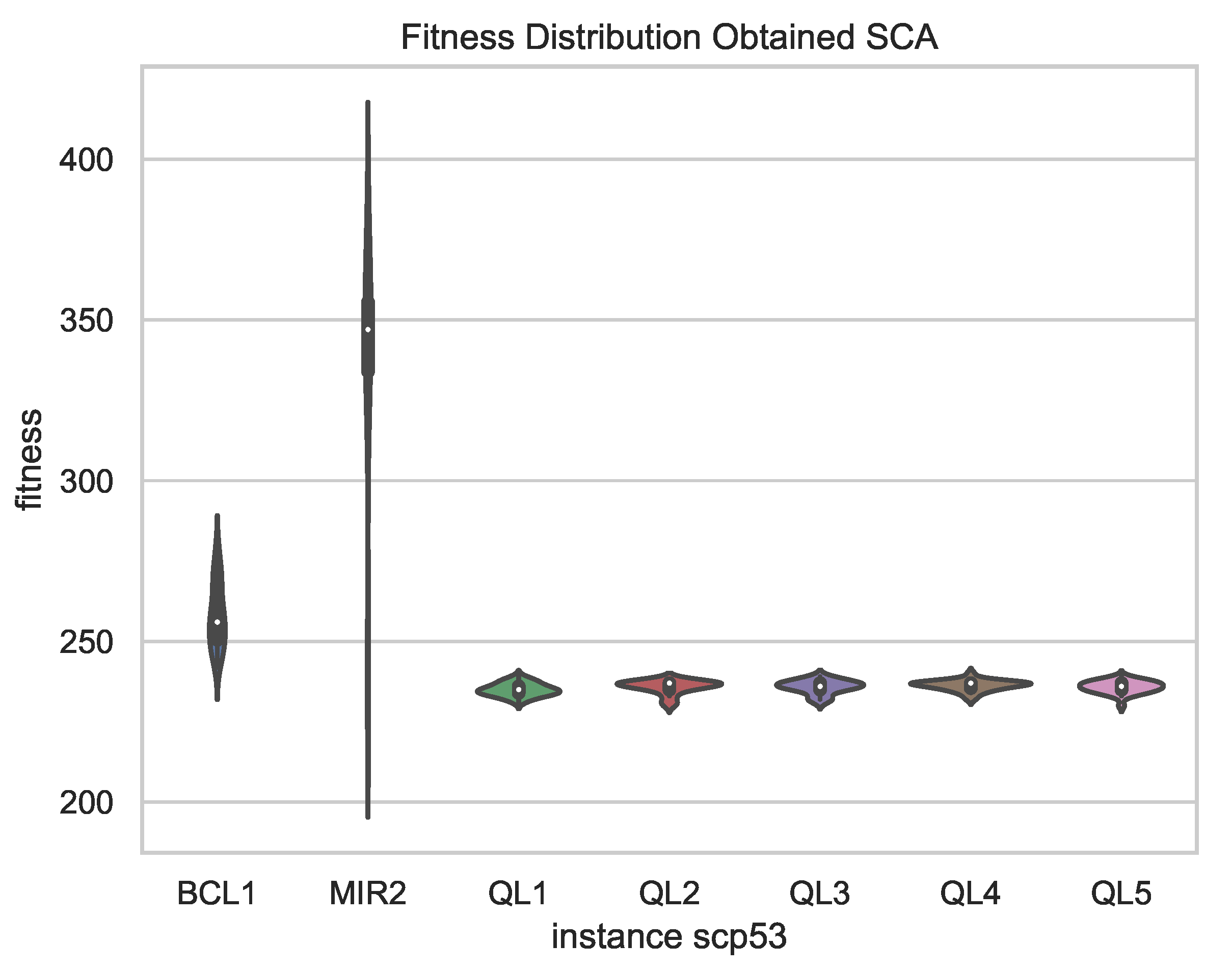
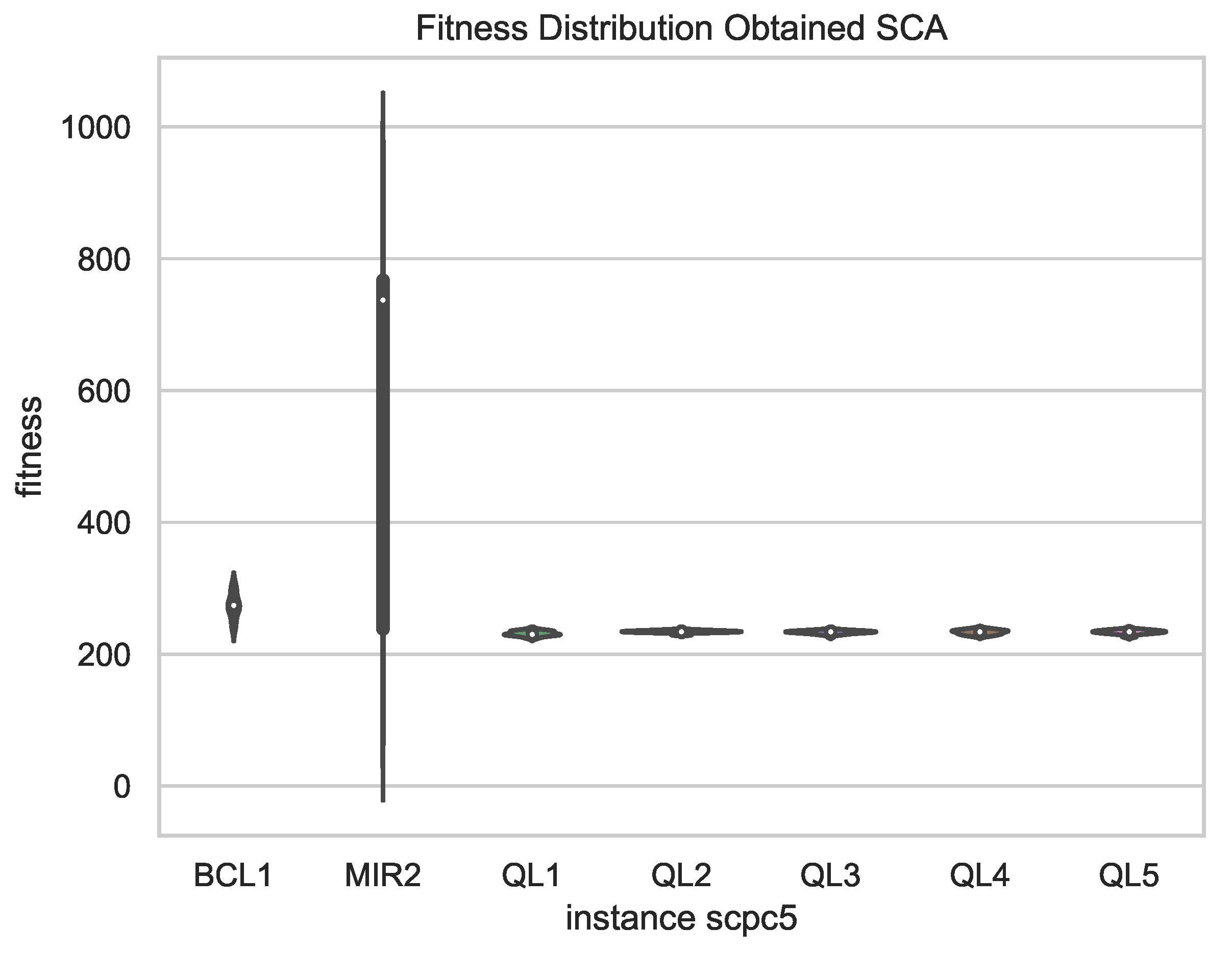
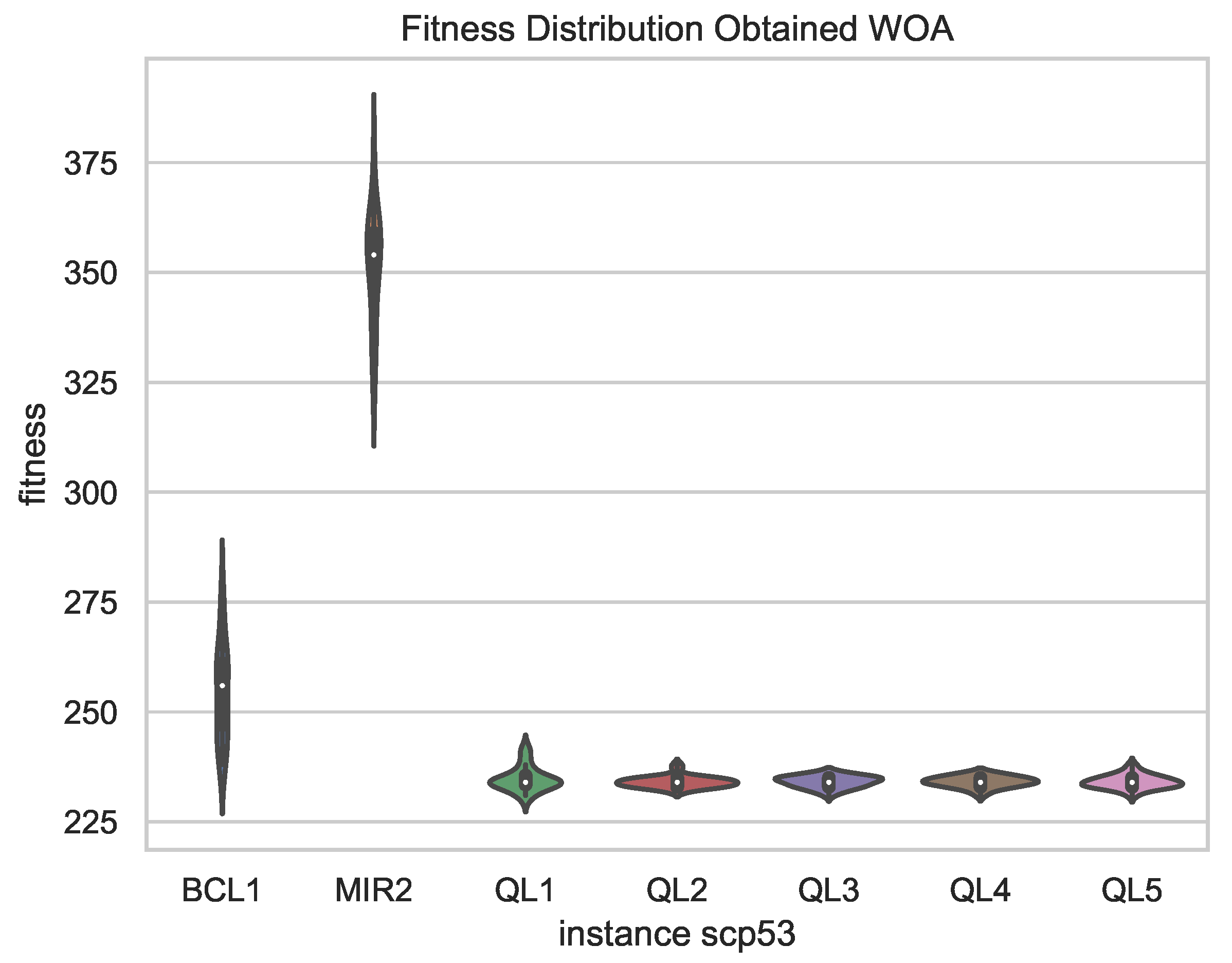
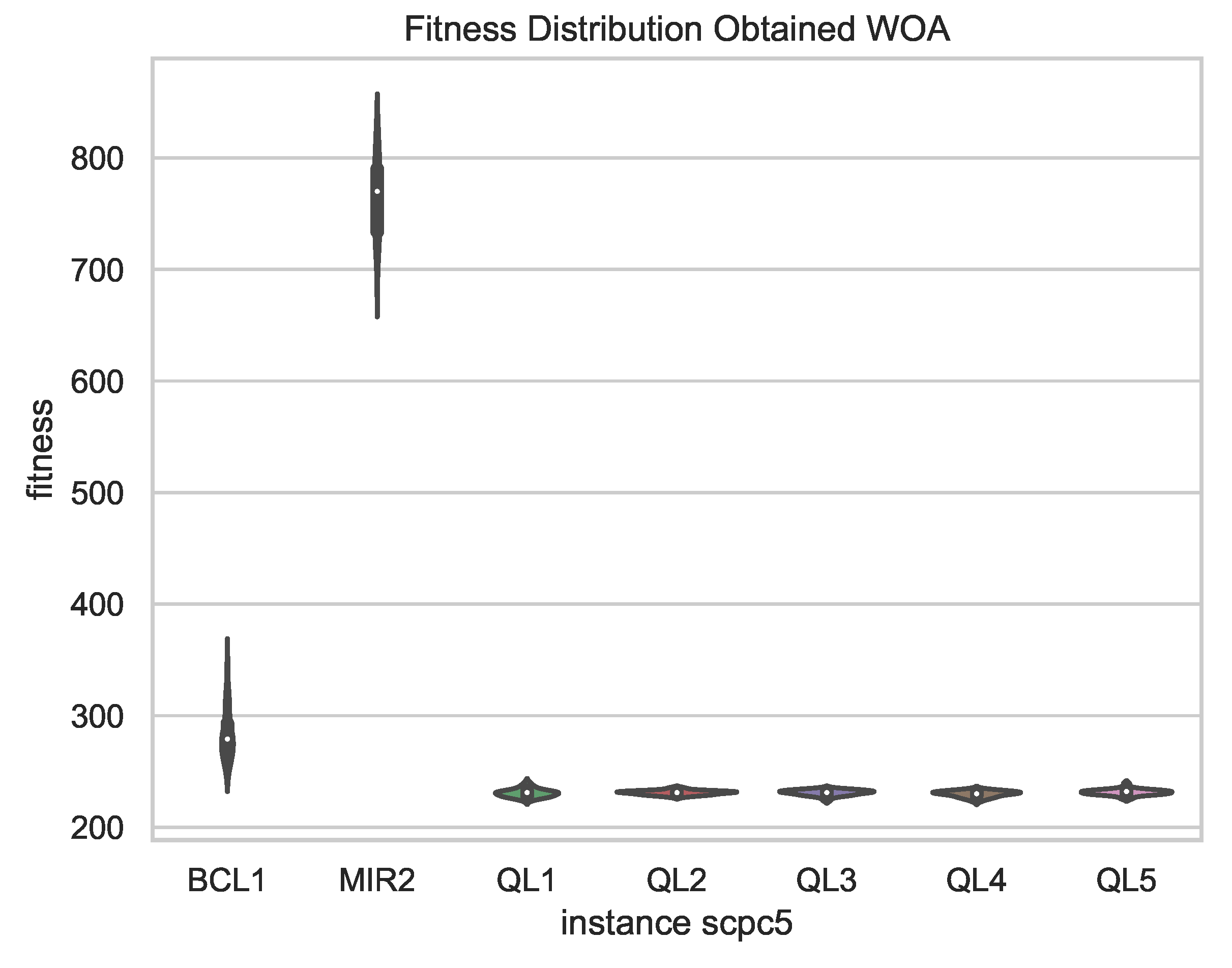
In Figure 5, Figure 6, Figure 7 and Figure 8, a comparison of the best results obtained in 31 independent runs of the chosen schemes is presented, showing less dispersion in the results for the versions with QL, which supports the robustness of the proposal compared to fixed binarization schemes, since, in addition to obtaining better results, these vary in smaller magnitude in independent runs.

Figure 9, Figure 10, Figure 11, Figure 12, Figure 13, Figure 14, Figure 15 and Figure 16, show the exploration and exploitation balance obtained by the algorithm. The x-axis represents the total number of iterations, the y-axis shows the percentage of exploration and exploitation, measured by Equations (20)–(22).

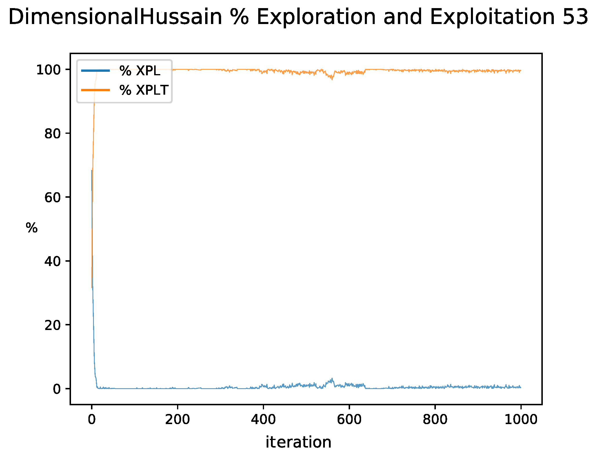
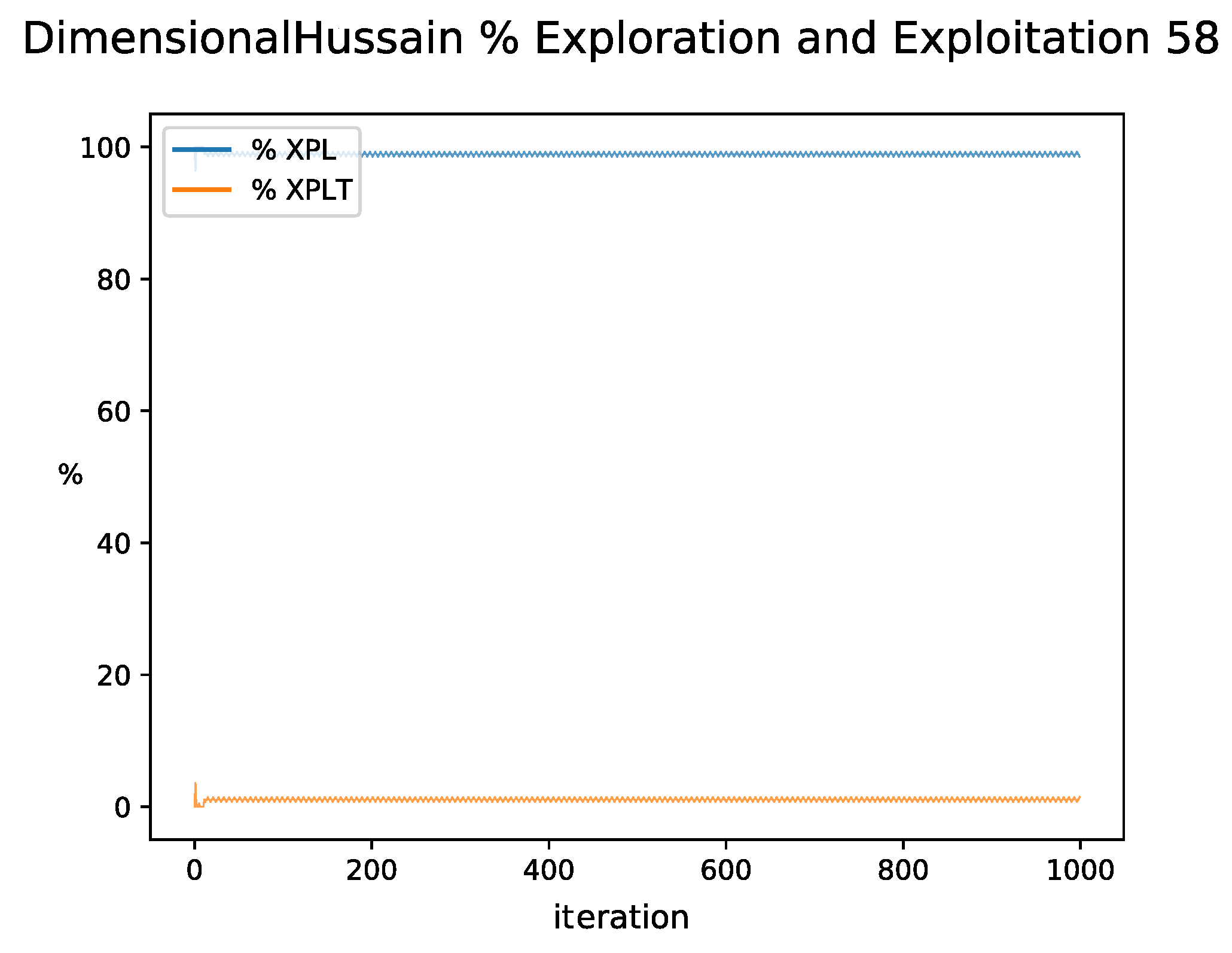
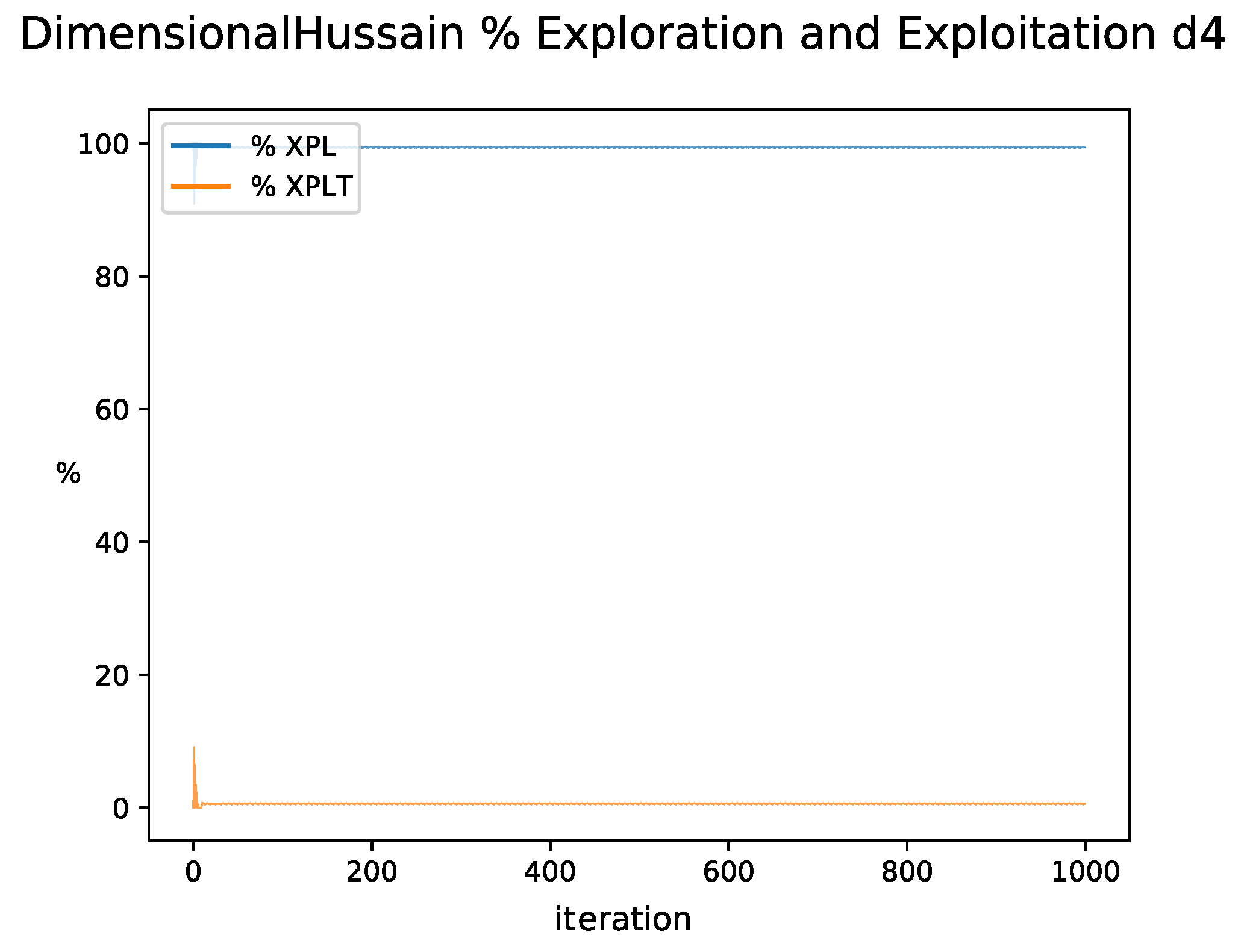
By observing the behavior of the exploration and exploitation percentages in the figures, it can be clearly observed that there are two different behaviors. In the case of Figure 10 and Figure 12, there is a clear beginning of exploration in the first iterations, while the exploitation increases until maintaining high values during the rest of the iterations. This behavior is the one recommended by [4], while for the case of Figure 14 and Figure 16, the exploration percentage remains at high values during all iterations and similar behavior is observed when random searches occur. For the versions with QL, the expected exploration and exploitation behavior is observed, where exploration predominates at the beginning and gradually changes to exploitation. However, in this one, variations in the percentages are observed given by the dynamic change of the binarization scheme in each iteration, which in turn has been reflected in better quality results.

These variations in exploration and exploitation percentages open the discussion about the implications of changing real-time binarization schemes, quantifying these percentage variations and the question of how to assess the quality of these changes.

8. Conclusions

Today, Machine Learning techniques are increasingly used in most areas of research, as data capture has been steadily increasing in recent years. MH have not been the exception, where these ML techniques have supported MH from various approaches in order to improve their performance. This is one of the main motivations for this proposal, since MH generate a large amount of data that is not always used for their operation. In the brief review of QL implementations, it is shown how this technique improves the performance of MH, managing to identify two methods of implementation: (1) as a selector of low-level heuristics in the context of hyperheuristics; (2) as a selector of a certain operator among a set of operators, as is the example of the choice of a mutation operator among different mutation operators. On the other hand, it is noted that the size of the Q-Table tends to take small sizes, since the sets of operators to be selected are usually small compared to other techniques of Machine Learning that address large amounts of input variables. The use of enhancements and combinations of QL with other Temporal Difference techniques such as SARSA (State-Action-Reward-State-Action) is also identified.

The algorithms presented in this work have shown that the choice of binarization schemes affects the balance of exploration and exploitation turning them into balanced metaheuristics [95], used in [96,97,98]. The balance achieved by our method shows an improvement in the quality of solutions, obtaining statistically significant better results.

Under the results obtained, it can be concluded that the versions that have incorporated QL in the selection of binarization schemes obtained variations in the percentages of exploration and exploitation, which are reflected in improvements in the quality of the solutions and in the techniques that do not present these disturbances in their static versions. These perturbations can be associated with better quality movements that will present a greater probability of finding better values when presenting variations in the percentages of exploration and exploitation, meaning that the solutions will have a greater rate of movement in the search space.

On the other hand, when observing the comparison between the average execution times (“Sec” column in Table 3 and Table 4), a great increase in time is observed for the versions that incorporate the binarization scheme selector, which are approximately around 447% in WOA and 223% for SCA; this is justifiable since the incorporation of QL to the iterative process of the MH, means a greater demand of calculation, since in each iteration the decision of which binarization scheme to use must be taken. However, this difference in time when comparing against a single binarization scheme, among the 40 combinations that were already explained in Section 3, produces an unequal comparison. Moreover, by not having a selector of binarization schemes, the 40 combinations of binarization schemes presented in this work should be tested, but since this would involve too much computation time, recommendations presented in the literature are usually used; however, they do not ensure to be the best binarization scheme for the problem and techniques implemented. Consequently, our proposal of a binarization scheme selector is of greater relevance since the high computational costs for the choice of binarization schemes are often not affordable; thus, under this scenario our proposal excels when compared with fixed binarization schemes.

In terms of future work, the option of evaluating other MH with exploration and exploitation behaviors similar to those presented will be contemplated, as well as other more established MH such as Differential Evolution (DE) and Particle Swarm Optimization (PSO) in order to verify that the incorporation of QL generates the same effect on them. We also consider the evaluation of other Temporal Difference techniques to compete with QL, the inclusion of other existing transfer functions in the literature, such as O-Shapes, and the evaluation of other methods of rewarding in addition to the five we have evaluated in the present work.

References

- Talbi, E. Metaheuristics: From Design to Implementation; John Wiley & Sons: Hoboken, NJ, USA, 2009; Volume 74. [Google Scholar]
- Xu, J.; Zhang, J. Exploration-exploitation tradeoffs in metaheuristics: Survey and analysis. In Proceedings of the 33rd Chinese Control Conference, Nanjing, China, 28–30 July 2014; pp. 8633–8638. [Google Scholar]
- Yang, X.S.; Deb, S.; Fong, S. Metaheuristic algorithms: Optimal balance of intensification and diversification. Appl. Math. Inf. Sci. 2014, 8, 977. [Google Scholar] [CrossRef]
- Morales-Castañeda, B.; Zaldivar, D.; Cuevas, E.; Fausto, F.; Rodríguez, A. A better balance in metaheuristic algorithms: Does it exist? Swarm Evol. Comput. 2020, 54, 100671. [Google Scholar] [CrossRef]
- Eftimov, T.; Korošec, P. Understanding exploration and exploitation powers of meta-heuristic stochastic optimization algorithms through statistical analysis. In Proceedings of the Genetic and Evolutionary Computation Conference Companion, Prague, Czech Republic, 13–17 July 2019; pp. 21–22. [Google Scholar]
- Hussain, A.; Muhammad, Y.S. Trade-off between exploration and exploitation with genetic algorithm using a novel selection operator. Complex Intell. Syst. 2019, 6, 1–14. [Google Scholar] [CrossRef] [Green Version]
- Glover, F.; Samorani, M. Intensification, Diversification and Learning in metaheuristic optimization. J. Heuristics 2019, 25, 517–520. [Google Scholar] [CrossRef] [Green Version]
- Hussain, K.; Salleh, M.N.M.; Cheng, S.; Shi, Y. On the exploration and exploitation in popular swarm-based metaheuristic algorithms. Neural Comput. Appl. 2019, 31, 7665–7683. [Google Scholar] [CrossRef]
- Liu, H.L.; Chen, L.; Deb, K.; Goodman, E.D. Investigating the effect of imbalance between convergence and diversity in evolutionary multiobjective algorithms. IEEE Trans. Evol. Comput. 2016, 21, 408–425. [Google Scholar]
- Gendreau, M.; Potvin, J.Y. Handbook of Metaheuristics; International Series in Operations Research & Management Science; Springer: Cham, Switzerland, 2019; Volume 272. [Google Scholar] [CrossRef]
- Crawford, B.; Soto, R.; Astorga, G.; Lemus-Romani, J.; Misra, S.; Rubio, J.M. An adaptive intelligent water drops algorithm for set covering problem. In Proceedings of the 2019 19th International Conference on Computational Science and Its Applications (ICCSA), St. Petersburg, Russia, 1–4 July 2019; pp. 39–45. [Google Scholar]
- Crawford, B.; Soto, R.; Olivares, R.; Embry, G.; Flores, D.; Palma, W.; Castro, C.; Paredes, F.; Rubio, J.M. A binary monkey search algorithm variation for solving the set covering problem. Nat. Comput. 2019, 19, 825–841. [Google Scholar] [CrossRef]
- García, J.; Crawford, B.; Soto, R.; Castro, C.; Paredes, F. A k-means binarization framework applied to multidimensional knapsack problem. Appl. Intell. 2018, 48, 357–380. [Google Scholar] [CrossRef]
- Crawford, B.; Soto, R.; Astorga, G.; Lemus, J.; Salas-Fernández, A. Self-configuring Intelligent Water Drops Algorithm for Software Project Scheduling Problem. In International Conference on Information Technology & Systems; Springer: Cham, Switzerland, 2019; pp. 274–283. [Google Scholar]
- Crawford, B.; Soto, R.; Astorga, G.; Castro, C.; Paredes, F.; Misra, S.; Rubio, J.M. Solving the software project scheduling problem using intelligent water drops. Teh. Vjesn. 2018, 25, 350–357. [Google Scholar]
- Mafarja, M.M.; Mirjalili, S. Hybrid whale optimization algorithm with simulated annealing for feature selection. Neurocomputing 2017, 260, 302–312. [Google Scholar] [CrossRef]
- Ho, Y.C.; Pepyne, D.L. Simple explanation of the no-free-lunch theorem and its implications. J. Optim. Theory Appl. 2002, 115, 549–570. [Google Scholar] [CrossRef]
- Crawford, B.; Soto, R.; Astorga, G.; García, J.; Castro, C.; Paredes, F. Putting continuous metaheuristics to work in binary search spaces. Complexity 2017, 2017, 8404231. [Google Scholar] [CrossRef] [Green Version]
- García, J.; Moraga, P.; Valenzuela, M.; Crawford, B.; Soto, R.; Pinto, H.; Peña, A.; Altimiras, F.; Astorga, G. A Db-Scan Binarization Algorithm Applied to Matrix Covering Problems. Comput. Intell. Neurosci. 2019, 2019, 3238574. [Google Scholar] [CrossRef] [Green Version]
- Maniezzo, V.; Stützle, T.; Voß, S. (Eds.) Matheuristics—Volume 10 of Annals of Information Systems; Springer: Berlin/Heidelberg, Germany, 2010. [Google Scholar]
- Juan, A.A.; Faulin, J.; Grasman, S.E.; Rabe, M.; Figueira, G. A review of simheuristics: Extending metaheuristics to deal with stochastic combinatorial optimization problems. Oper. Res. Perspect. 2015, 2, 62–72. [Google Scholar] [CrossRef] [Green Version]
- Juan, A.A.; Keenan, P.; Martı, R.; McGarraghy, S.; Panadero, J.; Carroll, P.; Oliva, D. A Review of the Role of Heuristics in Stochastic Optimisation: From Metaheuristics to Learnheuristics. Ann. Oper. Res. 2021. [Google Scholar] [CrossRef]
- Arnau, Q.; Juan, A.A.; Serra, I. On the use of learnheuristics in vehicle routing optimization problems with dynamic inputs. Algorithms 2018, 11, 208. [Google Scholar] [CrossRef] [Green Version]
- Bayliss, C.; Juan, A.A.; Currie, C.S.; Panadero, J. A learnheuristic approach for the team orienteering problem with aerial drone motion constraints. Appl. Soft Comput. 2020, 92, 106280. [Google Scholar] [CrossRef]
- Lavecchia, A. Machine-learning approaches in drug discovery: Methods and applications. Drug Discov. Today 2015, 20, 318–331. [Google Scholar] [CrossRef] [Green Version]
- Najafabadi, M.M.; Villanustre, F.; Khoshgoftaar, T.M.; Seliya, N.; Wald, R.; Muharemagic, E. Deep learning applications and challenges in big data analytics. J. Big Data 2015, 2, 1. [Google Scholar] [CrossRef] [Green Version]
- Kotsiantis, S.B.; Zaharakis, I.; Pintelas, P. Supervised machine learning: A review of classification techniques. Emerg. Artif. Intell. Appl. Comput. Eng. 2007, 160, 3–24. [Google Scholar]
- Celebi, M.E.; Aydin, K. Unsupervised Learning Algorithms; Springer: Berlin/Heidelberg, Germany, 2016; Volume 9. [Google Scholar]
- Valdivia, S.; Soto, R.; Crawford, B.; Caselli, N.; Paredes, F.; Castro, C.; Olivares, R. Clustering-based binarization methods applied to the crow search algorithm for 0/1 combinatorial problems. Mathematics 2020, 8, 1070. [Google Scholar] [CrossRef]
- Lorbeer, B.; Kosareva, A.; Deva, B.; Softić, D.; Ruppel, P.; Küpper, A. Variations on the clustering algorithm BIRCH. Big Data Res. 2018, 11, 44–53. [Google Scholar] [CrossRef]
- Chapelle, O.; Scholkopf, B.; Zien, A. Semi-supervised learning (chapelle, o. et al., eds.; 2006) [book reviews]. IEEE Trans. Neural Netw. 2009, 20, 542. [Google Scholar] [CrossRef]
- Sutton, R.S.; Barto, A.G. Reinforcement Learning: An Introduction; MIT Press: Cambridge, MA, USA, 2018. [Google Scholar]
- Veček, N.; Mernik, M.; Filipič, B.; Črepinšek, M. Parameter tuning with Chess Rating System (CRS-Tuning) for meta-heuristic algorithms. Inf. Sci. 2016, 372, 446–469. [Google Scholar] [CrossRef]
- Ries, J.; Beullens, P. A semi-automated design of instance-based fuzzy parameter tuning for metaheuristics based on decision tree induction. J. Oper. Res. Soc. 2015, 66, 782–793. [Google Scholar] [CrossRef] [Green Version]
- Deng, Y.; Liu, Y.; Zhou, D. An improved genetic algorithm with initial population strategy for symmetric TSP. Math. Probl. Eng. 2015, 2015, 212794. [Google Scholar] [CrossRef] [Green Version]
- García, J.; Crawford, B.; Soto, R.; Astorga, G. A percentile transition ranking algorithm applied to binarization of continuous swarm intelligence metaheuristics. In International Conference on Soft Computing and Data Mining; Springer: Cham, Switzerland, 2018; pp. 3–13. [Google Scholar]
- García, J.; Altimiras, F.; Peña, A.; Astorga, G.; Peredo, O. A binary cuckoo search big data algorithm applied to large-scale crew scheduling problems. Complexity 2018, 2018, 8395193. [Google Scholar] [CrossRef]
- de León, A.D.; Lalla-Ruiz, E.; Melián-Batista, B.; Moreno-Vega, J.M. A Machine Learning-based system for berth scheduling at bulk terminals. Expert Syst. Appl. 2017, 87, 170–182. [Google Scholar] [CrossRef]
- Asta, S.; Özcan, E.; Curtois, T. A tensor based hyper-heuristic for nurse rostering. Knowl. Based Syst. 2016, 98, 185–199. [Google Scholar] [CrossRef] [Green Version]
- Martin, S.; Ouelhadj, D.; Beullens, P.; Ozcan, E.; Juan, A.A.; Burke, E.K. A multi-agent based cooperative approach to scheduling and routing. Eur. J. Oper. Res. 2016, 254, 169–178. [Google Scholar] [CrossRef] [Green Version]
- Song, H.; Triguero, I.; Özcan, E. A review on the self and dual interactions between machine learning and optimisation. Prog. Artif. Intell. 2019, 8, 143–165. [Google Scholar] [CrossRef] [Green Version]
- Zhang, H.; Lu, J. Adaptive evolutionary programming based on reinforcement learning. Inf. Sci. 2008, 178, 971–984. [Google Scholar] [CrossRef]
- Dorigo, M.; Birattari, M.; Stutzle, T. Ant colony optimization. IEEE Comput. Intell. Mag. 2006, 1, 28–39. [Google Scholar] [CrossRef] [Green Version]
- Gambardella, L.M.; Dorigo, M. Ant-Q: A reinforcement learning approach to the traveling salesman problem. In Machine Learning Proceedings 1995; Elsevier: Amsterdam, The Netherlands, 1995; pp. 252–260. [Google Scholar]
- Khamassi, I.; Hammami, M.; Ghédira, K. Ant-q hyper-heuristic approach for solving 2-dimensional cutting stock problem. In Proceedings of the 2011 IEEE Symposium on Swarm Intelligence, Paris, France, 11–15 April 2011; pp. 1–7. [Google Scholar]
- Choong, S.S.; Wong, L.P.; Lim, C.P. Automatic design of hyper-heuristic based on reinforcement learning. Inf. Sci. 2018, 436, 89–107. [Google Scholar] [CrossRef]
- Mosadegh, H.; Ghomi, S.F.; Süer, G. Stochastic mixed-model assembly line sequencing problem: Mathematical modeling and Q-learning based simulated annealing hyper-heuristics. Eur. J. Oper. Res. 2020, 282, 530–544. [Google Scholar] [CrossRef]
- Burke, E.K.; Gendreau, M.; Hyde, M.; Kendall, G.; McCollum, B.; Ochoa, G.; Parkes, A.J.; Petrovic, S. The cross-domain heuristic search challenge—An international research competition. In International Conference on Learning and Intelligent Optimization; Springer: Cham, Switzerland, 2011; pp. 631–634. [Google Scholar]
- Li, Z.; Li, S.; Yue, C.; Shang, Z.; Qu, B. Differential evolution based on reinforcement learning with fitness ranking for solving multimodal multiobjective problems. Swarm Evol. Comput. 2019, 49, 234–244. [Google Scholar] [CrossRef]
- Alimoradi, M.R.; Kashan, A.H. A league championship algorithm equipped with network structure and backward Q-learning for extracting stock trading rules. Appl. Soft Comput. 2018, 68, 478–493. [Google Scholar] [CrossRef]
- Sadhu, A.K.; Konar, A.; Bhattacharjee, T.; Das, S. Synergism of firefly algorithm and Q-learning for robot arm path planning. Swarm Evol. Comput. 2018, 43, 50–68. [Google Scholar] [CrossRef]
- Zamli, K.Z.; Din, F.; Ahmed, B.S.; Bures, M. A hybrid Q-learning sine-cosine-based strategy for addressing the combinatorial test suite minimization problem. PLoS ONE 2018, 13, e0195675. [Google Scholar]
- Yang, X.S. Firefly Algorithms. Nature-Inspired Optimization Algorithms; Elsevier: Amsterdam, The Netherlands, 2021; pp. 123–139. [Google Scholar]
- Xu, Y.; Pi, D. A reinforcement learning-based communication topology in particle swarm optimization. Neural Comput. Appl. 2019, 32, 10007–10032. [Google Scholar] [CrossRef]
- Das, P.; Behera, H.; Panigrahi, B. Intelligent-based multi-robot path planning inspired by improved classical Q-learning and improved particle swarm optimization with perturbed velocity. Eng. Sci. Technol. Int. J. 2016, 19, 651–669. [Google Scholar] [CrossRef] [Green Version]
- Abed-alguni, B.H. Action-selection method for reinforcement learning based on cuckoo search algorithm. Arab. J. Sci. Eng. 2018, 43, 6771–6785. [Google Scholar] [CrossRef]
- Abed-alguni, B.H. Bat Q-learning algorithm. Jordanian J. Comput. Inf. Technol. (JJCIT) 2017, 3, 56–77. [Google Scholar]
- Arin, A.; Rabadi, G. Integrating estimation of distribution algorithms versus Q-learning into Meta-RaPS for solving the 0–1 multidimensional knapsack problem. Comput. Ind. Eng. 2017, 112, 706–720. [Google Scholar] [CrossRef]
- Mirjalili, S.; Lewis, A. S-shaped versus V-shaped transfer functions for binary particle swarm optimization. Swarm Evol. Comput. 2013, 9, 1–14. [Google Scholar] [CrossRef]
- Faris, H.; Mafarja, M.M.; Heidari, A.A.; Aljarah, I.; Ala’M, A.Z.; Mirjalili, S.; Fujita, H. An efficient binary salp swarm algorithm with crossover scheme for feature selection problems. Knowl. Based Syst. 2018, 154, 43–67. [Google Scholar] [CrossRef]
- Mafarja, M.; Aljarah, I.; Heidari, A.A.; Faris, H.; Fournier-Viger, P.; Li, X.; Mirjalili, S. Binary dragonfly optimization for feature selection using time-varying transfer functions. Knowl. Based Syst. 2018, 161, 185–204. [Google Scholar] [CrossRef]
- Mirjalili, S.; Hashim, S.Z.M. BMOA: Binary magnetic optimization algorithm. Int. J. Mach. Learn. Comput. 2012, 2, 204. [Google Scholar] [CrossRef] [Green Version]
- Crawford, B.; Soto, R.; Olivares-Suarez, M.; Palma, W.; Paredes, F.; Olguin, E.; Norero, E. A binary coded firefly algorithm that solves the set covering problem. Rom. J. Inf. Sci. Technol 2014, 17, 252–264. [Google Scholar]
- Crawford, B.; Soto, R.; Berríos, N.; Johnson, F.; Paredes, F.; Castro, C.; Norero, E. A binary cat swarm optimization algorithm for the non-unicost set covering problem. Math. Probl. Eng. 2015, 2015, 578541. [Google Scholar] [CrossRef] [Green Version]
- Soto, R.; Crawford, B.; Olivares, R.; Barraza, J.; Figueroa, I.; Johnson, F.; Paredes, F.; Olguin, E. Solving the non-unicost set covering problem by using cuckoo search and black hole optimization. Nat. Comput. 2017, 16, 213–229. [Google Scholar] [CrossRef]
- Soto, R.; Crawford, B.; Olivares, R.; Taramasco, C.; Figueroa, I.; Gómez, A.; Castro, C.; Paredes, F. Adaptive Black Hole Algorithm for Solving the Set Covering Problem. Math. Probl. Eng. 2018, 2018, 2183214. [Google Scholar] [CrossRef]
- Leonard, B.J.; Engelbrecht, A.P.; Cleghorn, C.W. Critical considerations on angle modulated particle swarm optimisers. Swarm Intell. 2015, 9, 291–314. [Google Scholar] [CrossRef]
- Zhang, G. Quantum-inspired evolutionary algorithms: A survey and empirical study. J. Heuristics 2011, 17, 303–351. [Google Scholar] [CrossRef]
- Saremi, S.; Mirjalili, S.; Lewis, A. How important is a transfer function in discrete heuristic algorithms. Neural Comput. Appl. 2015, 26, 625–640. [Google Scholar] [CrossRef] [Green Version]
- Kennedy, J.; Eberhart, R.C. A discrete binary version of the particle swarm algorithm. In Proceedings of the 1997 IEEE International conference on systems, man, and cybernetics. Computational cybernetics and simulation, Orlando, FL, USA, 12–15 October 1997; Volume 5, pp. 4104–4108. [Google Scholar]
- Rajalakshmi, N.; Subramanian, D.P.; Thamizhavel, K. Performance enhancement of radial distributed system with distributed generators by reconfiguration using binary firefly algorithm. J. Inst. Eng. (India) Ser. B 2015, 96, 91–99. [Google Scholar] [CrossRef]
- Crawford, B.; Soto, R.; Peña, C.; Riquelme-Leiva, M.; Torres-Rojas, C.; Johnson, F.; Paredes, F. Binarization methods for shuffled frog leaping algorithms that solve set covering problems. In Software Engineering in Intelligent Systems; Springer: Cham, Switzerland, 2015; pp. 317–326. [Google Scholar]
- Tamayo-Vera, D.; Chen, S.; Bolufé-Röhler, A.; Montgomery, J.; Hendtlass, T. Improved Exploration and Exploitation in Particle Swarm Optimization. In Recent Trends and Future Technology in Applied Intelligence; Mouhoub, M., Sadaoui, S., Ait Mohamed, O., Ali, M., Eds.; Springer International Publishing: Cham, Switzerland, 2018; pp. 421–433. [Google Scholar]
- Črepinšek, M.; Liu, S.H.; Mernik, M. Exploration and Exploitation in Evolutionary Algorithms: A Survey. ACM Comput. Surv. 2013, 45. [Google Scholar] [CrossRef]
- Olorunda, O.; Engelbrecht, A.P. Measuring exploration/exploitation in particle swarms using swarm diversity. In Proceedings of the 2008 IEEE Congress on Evolutionary Computation (IEEE World Congress on Computational Intelligence, Hong Kong, China, 1–6 June 2008; pp. 1128–1134. [Google Scholar] [CrossRef]
- Burke, E.K.; Hyde, M.R.; Kendall, G.; Ochoa, G.; Özcan, E.; Woodward, J.R. A Classification of Hyper-Heuristic Approaches: Revisited. In Handbook of Metaheuristics; Gendreau, M., Potvin, J.Y., Eds.; Springer International Publishing: Cham, Switzerland, 2019; pp. 453–477. [Google Scholar] [CrossRef]
- Oyebolu, F.B.; Allmendinger, R.; Farid, S.S.; Branke, J. Dynamic scheduling of multi-product continuous biopharmaceutical facilities: A hyper-heuristic framework. Comput. Chem. Eng. 2019, 125, 71–88. [Google Scholar] [CrossRef] [Green Version]
- Leng, L.; Zhao, Y.; Wang, Z.; Zhang, J.; Wang, W.; Zhang, C. A Novel Hyper-Heuristic for the Biobjective Regional Low-Carbon Location-Routing Problem with Multiple Constraints. Sustainability 2019, 11, 1596. [Google Scholar] [CrossRef] [Green Version]
- Watkins, C.J.; Dayan, P. Q-learning. Mach. Learn. 1992, 8, 279–292. [Google Scholar] [CrossRef]
- Nareyek, A. Choosing search heuristics by non-stationary reinforcement learning. In Metaheuristics: Computer Decision-Making; Springer: Boston, MA, USA, 2003; pp. 523–544. [Google Scholar]
- Salleh, M.N.M.; Hussain, K.; Cheng, S.; Shi, Y.; Muhammad, A.; Ullah, G.; Naseem, R. Exploration and exploitation measurement in swarm-based metaheuristic algorithms: An empirical analysis. In International Conference on Soft Computing and Data Mining; Springer: Cham, Switzerland, 2018; pp. 24–32. [Google Scholar]
- Cheng, S.; Shi, Y.; Qin, Q.; Zhang, Q.; Bai, R. Population Diversity Maintenance In Brain Storm Optimization Algorithm. J. Artif. Intell. Soft Comput. Res. 2014, 4, 83–97. [Google Scholar] [CrossRef] [Green Version]
- Mattiussi, C.; Waibel, M.; Floreano, D. Measures of diversity for populations and distances between individuals with highly reorganizable genomes. Evol. Comput. 2004, 12, 495–515. [Google Scholar] [CrossRef] [Green Version]
- Lynn, N.; Suganthan, P.N. Heterogeneous comprehensive learning particle swarm optimization with enhanced exploration and exploitation. Swarm Evol. Comput. 2015, 24, 11–24. [Google Scholar] [CrossRef]
- Hussain, K.; Zhu, W.; Salleh, M.N.M. Long-term memory Harris’ hawk optimization for high dimensional and optimal power flow problems. IEEE Access 2019, 7, 147596–147616. [Google Scholar] [CrossRef]
- Abualigah, L.; Diabat, A. Advances in Sine Cosine Algorithm: A comprehensive survey. Artif. Intell. Rev. 2021, 54, 2567–2608. [Google Scholar] [CrossRef]
- Mirjalili, S.; Mirjalili, S.M.; Saremi, S.; Mirjalili, S. Whale optimization algorithm: Theory, literature review, and application in designing photonic crystal filters. Nat. Inspired Optim. 2020, 219–238. [Google Scholar] [CrossRef]
- Wolpert, D.H.; Macready, W.G. No free lunch theorems for optimization. IEEE Trans. Evol. Comput. 1997, 1, 67–82. [Google Scholar] [CrossRef] [Green Version]
- Mirjalili, S. SCA: A sine cosine algorithm for solving optimization problems. Knowl. Based Syst. 2016, 96, 120–133. [Google Scholar] [CrossRef]
- Mirjalili, S.; Lewis, A. The whale optimization algorithm. Adv. Eng. Softw. 2016, 95, 51–67. [Google Scholar] [CrossRef]
- Hassan, A.A.; Abdullah, S.; Zamli, K.Z.; Razali, R. Combinatorial Test Suites Generation Strategy Utilizing the Whale Optimization Algorithm. IEEE Access 2020, 9, 192288–192303. [Google Scholar] [CrossRef]
- Lanza-Gutierrez, J.M.; Crawford, B.; Soto, R.; Berrios, N.; Gomez-Pulido, J.A.; Paredes, F. Analyzing the effects of binarization techniques when solving the set covering problem through swarm optimization. Expert Syst. Appl. 2017, 70, 67–82. [Google Scholar] [CrossRef]
- Osaba, E.; Carballedo, R.; Diaz, F.; Onieva, E.; Masegosa, A.D.; Perallos, A. Good practice proposal for the implementation, presentation, and comparison of metaheuristics for solving routing problems. Neurocomputing 2018, 271, 2–8. [Google Scholar] [CrossRef] [Green Version]
- Bisong, E. Google colaboratory. In Building Machine Learning and Deep Learning Models on Google Cloud Platform; Springer: Berlin/Heidelberg, Germany, 2019; pp. 59–64. [Google Scholar]
- Crawford, B.; León de la Barra, C. Los Algoritmos Ambidiestros. 2020. Available online: https://www.mercuriovalpo.cl/impresa/2020/07/13/full/cuerpo-principal/15/ (accessed on 12 February 2021).
- Lemus-Romani, J.; Crawford, B.; Soto, R.; Astorga, G.; Misra, S.; Crawford, K.; Foschino, G.; Salas-Fernández, A.; Paredes, F. Ambidextrous Socio-Cultural Algorithms. In International Conference on Computational Science and Its Applications; Springer: Cham, Switzerland, 2020; pp. 923–938. [Google Scholar]
- Cisternas-Caneo, F.; Crawford, B.; Soto, R.; de la Fuente-Mella, H.; Tapia, D.; Lemus-Romani, J.; Castillo, M.; Becerra-Rozas, M.; Paredes, F.; Misra, S. A Data-Driven Dynamic Discretization Framework to Solve Combinatorial Problems Using Continuous Metaheuristics. In Innovations in Bio-Inspired Computing and Applications; Springer International Publishing: Cham, Switzerland, 2021; pp. 76–85. [Google Scholar]
- Tapia, D.; Crawford, B.; Soto, R.; Cisternas-Caneo, F.; Lemus-Romani, J.; Castillo, M.; García, J.; Palma, W.; Paredes, F.; Misra, S. A Q-Learning Hyperheuristic Binarization Framework to Balance Exploration and Exploitation. In International Conference on Applied Informatics; Springer: Cham, Switzerland, 2020; pp. 14–28. [Google Scholar]