A Neural Network Technique for the Derivation of Runge–Kutta Pairs Adjusted for Scalar Autonomous Problems

Abstract

We consider the scalar autonomous initial value problem as solved by an explicit Runge–Kutta pair of orders 6 and 5. We focus on an efficient family of such pairs, which were studied extensively in previous decades. This family comes with 5 coefficients that one is able to select arbitrarily. We set, as a fitness function, a certain measure, which is evaluated after running the pair in a couple of relevant problems. Thus, we may adjust the coefficients of the pair, minimizing this fitness function using the differential evolution technique. We conclude with a method (i.e. a Runge–Kutta pair) which outperforms other pairs of the same two orders in a variety of scalar autonomous problems.

1. Introduction

The Initial Value Problem (IVP) is given as

$$\begin{array}{ccc}\hfill x^{\prime }& =& f(t,x),\hfill \\ \hfill x(t_0)& =& x_0\hfill \end{array}$$

(1)

with $t,t_0\in IR$, $x,x^{\prime }\in I{R}^m$ and $f:IR\times I{R}^m\to I{R}^m.$

Amongst the most celebrated numerical methods for dealing with (1) are Runge–Kutta (RK) pairs. The following Butcher tableau [1,2] characterizes these methods.

$$\begin{array}{cc}\hfill a& B\\ & c\\ & \widehat{c}\end{array}$$

with $c^T,{\widehat{c}}^T,a\in I{R}^s$ and $B\in I{R}^{s\times s}.$ In the above case, the pair shares s stages that are evaluated explicitly when B is strictly lower triangular. The approximation of the solution, forwards from $(t_n,x_n)$ to $t_{n+1}=t_n+h_n$ is furnished by two estimations of $x(t_{n+1}).$ These are $x_{n+1}$ and ${\widehat{x}}_{n+1}$, which are given by

$$x_{n+1}=x_n+h_n·\sum _{i=1}^{i=s}{c}_i{k}_i$$

with

$${\widehat{x}}_{n+1}=x_n+h_n·\sum _{i=1}^{i=s}{\widehat{c}}_i{k}_i$$

and

$$k_i=f(t_n+a_i{h}_n,x_n+h_n·\sum _{j=1}^{j=i-1}{b}_{ij}{k}_j),$$

for $i=1,2,\cdots ,s.$ The approximations $x_{n+1}$ and ${\widehat{x}}_{n+1}$ are of algebraic orders p and $q<p$, respectively. Thus, a local error estimation

$${ϵ}_n=h_n^{p-q-1}·\parallel x_{n+1}-{\widehat{x}}_{n+1}\parallel ,$$

is formed in every step. This helps in forming the following step changing algorithm

$$h_{n+1}=d·h_n^{}·{(\frac{\sigma }{{ϵ}_n})}^{1/p},$$

where $\sigma$ is a tolerance, chosen by the user, and $d=0.9$ is a safety factor. In the case that ${ϵ}_n<\sigma$, the above formula is used as the next step–length. On the contrary, we also use this formula, but the approximate solution is not forwarded and $h_{n+1}$ is used as new version of $h_n$. Details of this issue can be retrieved from [3] or even [4] (pg. 167–168). These methods are usually abbreviated as RKp(q) pairs.

Runge–Kutta methods first appeared in the late nineteenth century [5,6], while pairs were introduced after 1960. The first-celebrated such pairs, of orders 5(4), 6(5) and 8(7), were presented by Fehlberg [7,8]. Then, in the early 1980’s, Dormand and Prince followed [9,10]. In addition, our research group has derived a number of such pairs [11,12,13,14].

Runge–Kutta pairs are well suited for efficiently approximating the solution of non-stiff problems of the form in (1). Such problems arise, for example, when creating digital twins of clean-energy production technologies, for which functionally fitted finite element methods, with one-step and multi-step forms and improved dispersive and dissipative properties, have become critically important [15]. The precision demanded explains the wide diversity of pairs. As a result, the lower the accuracy on demand, the more efficient the lower RK pairs are. In reverse, a higher-order pair should be used for stringent accuracies at quadruple precision. [16]. The effort to construct better pairs is the subject of current research [17,18].

Here, we focus on RK6(5) pairs, which are used for high to modest accuracies. We are especially interested in problems (1) of the form

$$x^{\prime }=f(x),x(t_0)=x_0,$$

(2)

with $f:IR\to IR.$ These problems are called scalar autonomous, and we will derive a particular RK6(5) pair tuned specially for this type of problem.

The paper is organized into sections as follows:

• Introduction;
• Theory of Runge–Kutta Pairs of Orders 6(5);
• Training the coefficients;
• Numerical Tests;
• Conclusions.

2. Theory of Runge–Kutta Pairs of Orders 6(5)

Runge–Kutta pairs of orders six and five are, almost, the most-used ones. Their coefficients have to satisfy 54 order conditions, and families of solutions have been discovered through the years. We have selected the Verner-DLMP [19,20] family, which has the advantage of being solved linearly. This is an FSAL (First Stage As Last) family. Although $s=9,$ the pairs use only eight stages each step, since the last (the 9th) stage is used as the first stage of the next step.

Then we choose freely the coefficients $a_2,a_4,$$a_5,$$a_6,$$a_7$ and ${\widehat{c}}_9.$ This family’s pairs have been shown to perform the best in a variety of problems [21].

We may proceed by evaluating explicitly the remaining coefficients.

In the following algorithm $a^i$ is the vector with the components of a raised to the i-th power and $e={\left[1,1,\cdots ,1\right]}^T\in I{R}^s$. ${(B·a)}_5$ is the 5-th component of $B·a$. See [22,23] for more details. $A=diag(a)$ and I is the identity matrix of proper dimension.

ALGORITHM: The free parameters are $a_2,a_4,a_5,a_6,a_7,{\widehat{c}}_9$. It is known that for this family $c_2=c_3={\widehat{c}}_2={\widehat{c}}_3=0$ and $b_{i2}=0,i=4,5,6,7,8$. Consecutively execute the following instructions.

• Solve $c·e=1,c·a=\frac{1}{2},c·a^2=\frac{1}{3},c·a^3=\frac{1}{4},c·a^4=\frac{1}{5},c·a^5=\frac{1}{6}$, for $c_2,c_4,c_5,c_6,c_7,c_8$.
• Put $a_3={\displaystyle \frac{2}{3c_4}},b_{43}={\displaystyle \frac{a_4^2}{2a_3}},b_{32}={\displaystyle \frac{a_3^2}{2a_2}}$.
• Solve ${(b·a)}_5={\displaystyle \frac{a_5^2}{2}}$ and ${(b·a^2)}_5={\displaystyle \frac{a_5^3}{3}}$ for $b_{53},b_{54}$.
• Substitute $b_{87}$ from ${(c·(A+B-I))}_7=0$.
• Since ${(c·(A-I)·B)}_3=0$ find $b_{76}3ex-2ex$ from

  $$c·(A-I)·B·(A-a_{4}I)·(A-a_{5}I)·a-{(c(A-I)B)}_3={\int }_0^1(x-1){\int }_0^x(y-c_4)(y-c_5)ydydx.$$
• $b_{86}$ is given from ${(c·(B+A-I))}_6=0$.
• Solve simultaneously for ${\widehat{c}}_1,{\widehat{c}}_4,{\widehat{c}}_5,{\widehat{c}}_6,{\widehat{c}}_7,{\widehat{c}}_8$, $b_{63}$, $b_{73}$, and $b_{83}$ the equations:

  $$\widehat{c}·e=1,\widehat{c}·a=\frac{1}{2},\widehat{c}·a^2=\frac{1}{3},\widehat{c}·a^3=\frac{1}{4},\widehat{c}·a^4=\frac{1}{5},{(c·(B+A-I))}_3=0,{(\widehat{c}·B)}_3=0,$$

  $$c·(A-I)·B·(A-a_{4}I)·(A-a_{5}I)·a={\int }_0^1(x-1){\int }_0^x(y-a_5)(y-a_4)ydydx,$$

  $$\widehat{c}·B·(A-a_{5}I)·(A-a_{4}I)·a={\int }_0^1{\int }_0^x(y-a_5)(y-a_4)ydydx.$$
• From ${(B·a)}_6={\displaystyle \frac{a_6^2}{2}},{(B·a^2)}_6={\displaystyle \frac{a_6^3}{3}}$ evaluate $b_{64}$ and $b_{65}$.
• From ${(B·a)}_7=c_7^2/2,{(B·a^2)}_7=c_7^3/3$ evaluate $b_{74}$ and $b_{75}$.
• From ${(B·a)}_8=c_8^2/2,{(B·a^2)}_8=c_8^3/3$ evaluate $b_{84}$ and $b_{85}$.
• From $B·e=a$ evaluate $b_{21},b_{31},\cdots ,b_{81}$.
• Finally, using FSAL (First Stage As Last) property, substitute $b_{9j}=c_j,j=1,2,\cdots ,8$.

All equations are solved explicitly and straightforwardly. No back substitutions or implicit equations are present.

The question now raised is how to select the free parameters. Traditionally, we attempt to reduce the norm of the principal term of the local truncation error, i.e., the coefficients of $h^7$ in the residual of Taylor error expansions corresponding to the sixth order method of the underlying RK pair [11].

Another choice is examined in [24], where we dealt with a class of seven stages, as well as FSAL pairs of orders six and four, that are specially tuned for addressing the problems of interest here. We presented the reduced set of order conditions for the case of interest; then we solved it in order to furnish a certain pair ST6(4). We didn’t considered this case, since there are only two free parameters that are non-linearly dependent and it is not expected to make serious improvement. However, we will include this pair in our numerical tests.

3. Training the Coefficients

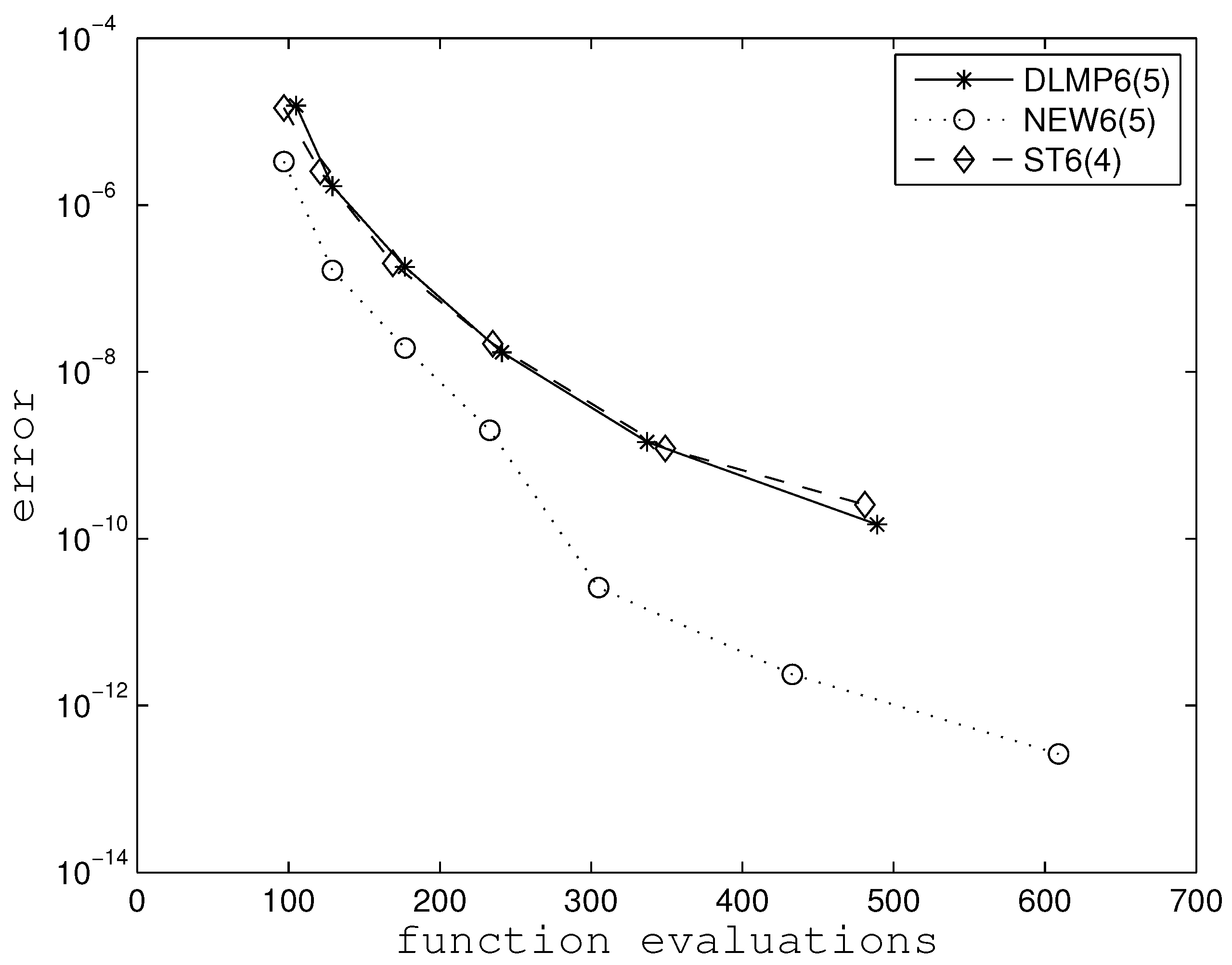
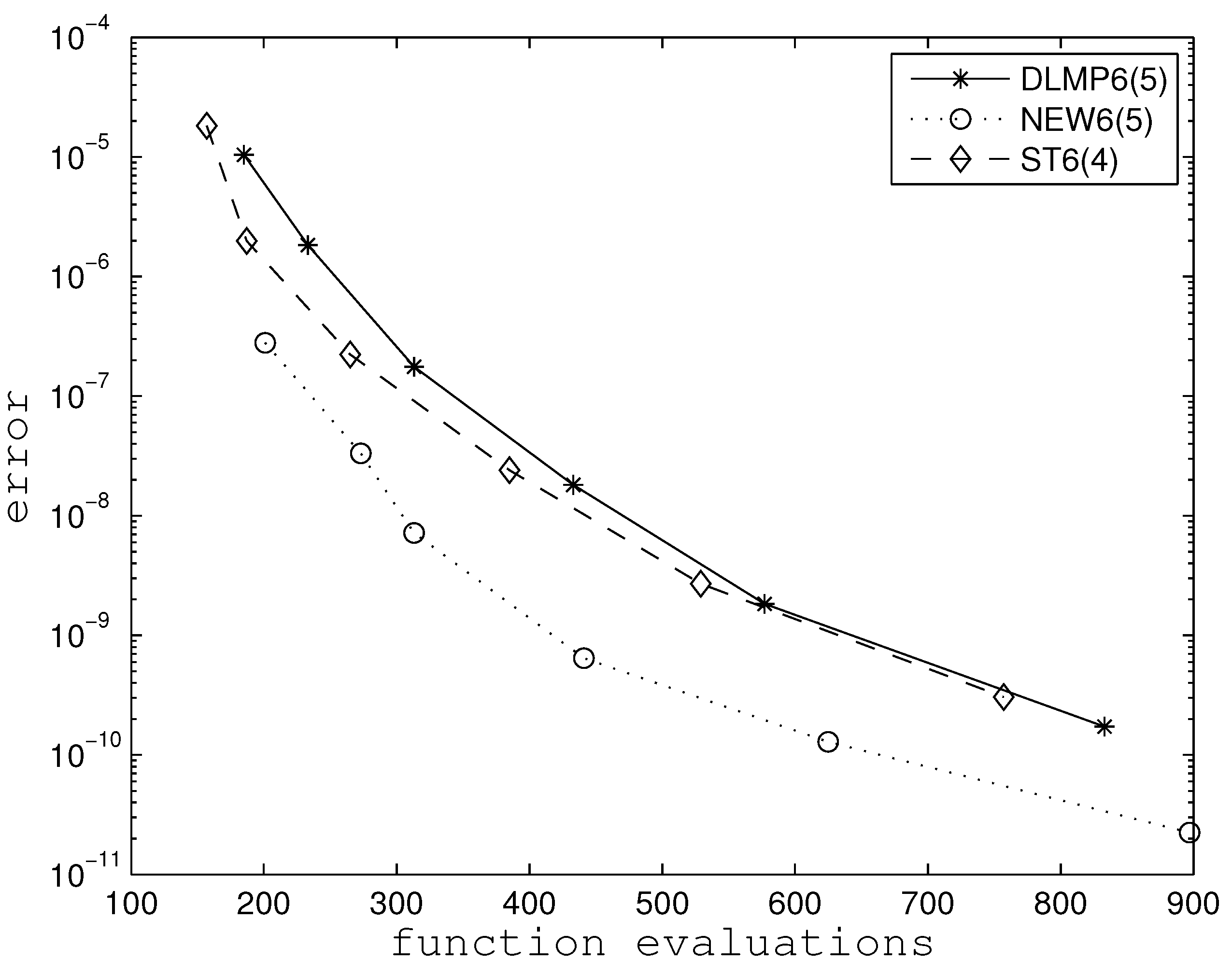
Here, our approach is to train the coefficients of a method. In this view, we say that we are utilizing a Neural Network technique. We consider, as input, the free parameters of the Runge–Kutta pair. Then, the steps taken for solving an Initial Value Problem can be seen as internal layers, while the output is a particular efficiency measure of the results.

We intend to derive a particular RK6(5) pair belonging to the studied family above. The resulting pair has to perform best on scalar autonomous problems (2). First, let us say that some pair was run in a certain problem (2) for some tolerance.

We then record the number $\mu$ of function evaluations (stages) needed and the global error $\epsilon$ observed over the whole mesh (grid-points) in the interval of integration. Then, we form the efficiency measure

$$r=\mu ·{\epsilon }^{1/6}.$$

(3)

Here we choose the following couple of scalar autonomous problems.

$$1\mathrm{st}\mathrm{problem}:x^{\prime }=e^{-x},x(0)=1,t\in [0,20],$$

with theoretical solution $x(t)=log(e+t)$, and

$$2\mathrm{nd}\mathrm{problem}:x^{\prime }=x^{1/3},x(0)=1,t\in [0,20],$$

with theoretical solution $x(t)=\frac{2}{3}\sqrt{\frac{2}{3}}·x^{3/2}$.

After using as tolerance $\sigma ={10}^{-11}$, we ran DLMP6(5) for the above problems. We recorded

$${\mu }_1=369,{\epsilon }_1\approx 1.9·{10}^{-12},{}^1{r}_{\mathrm{DLMP}65}=4.09,$$

for the first problem and

$${\mu }_2=433,{\epsilon }_2\approx 7.6·{10}^{-11},{}^2{r}_{\mathrm{DLMP}65}=8.92,$$

for the second problem.

Let us suppose that any new pair NEW6(5) furnishes corresponding efficiency measures ${}^1{r}_{\mathrm{NEW}65}$ and ${}^2{r}_{\mathrm{NEW}65}$ for the same runs. We then form, as a fitness function, the sum

$$\widehat{r}=\frac{{}^1{r}_{\mathrm{DLMP}65}}{{}^1{r}_{\mathrm{NEW}65}}+\frac{{}^2{r}_{\mathrm{DLMP}65}}{{}^w{r}_{\mathrm{NEW}65}},$$

(4)

and try to maximize it. That is, the compound fitness function is actually two whole runs of Initial Value Problems. The value $\widehat{r}$ changes according to the selection of the free parameters $a_2,a_4,$$a_5,$$a_6,$$a_7$ and ${\widehat{c}}_9.$

The original idea is based on [25]. For the minimization of $\widehat{r}$ we used the differential evolution technique [26]. We have already tried this approach and previously acquired some interesting results when producing Numerov-type methods for integrating orbits [27]. In that work, we trained the coefficients of a Numerov-type method on a Kepler orbit. We then observed excellent results over a set of Kepler orbits, as well other known orbital problems.

Software [28] was used for implementing our approach. As the objective (i.e. fitness) function we added (4). Actually, ${}^1{r}_{\mathrm{DLMP}65}$ and ${}^2{r}_{\mathrm{DLMP}65}$ were found in advance; ${}^1{r}_{\mathrm{NEW}65}$ and ${}^2{r}_{\mathrm{NEW}65}$ were adjusted according to the selection of the free parameters.

Finally, we derived an optimal method, named hereafter the NEW6(5) pair, sharing the following free parameters

$$a_2=0.010190841992960,a_4=0.119497020307147,$$

$$a_5=0.4156202137620401,a_6=0.574431750193581,$$

$$a_7=0.802904404563573,{\widehat{c}}_9=0.010038977481306$$

We ran this pair for tolerance $\sigma ={10}^{-11}$, and we recorded,

$${\mu }_1=305,{\epsilon }_1\approx 4.4·{10}^{-16},{}^1{r}_{\mathrm{NEW}65}=0.84,$$

for the first problem and

$${\mu }_2=297,{\epsilon }_2\approx 8.5·{10}^{-14},{}^2{r}_{\mathrm{NEW}65}=1.97,$$

for the second problem; i.e.,

$$\widehat{r}=\frac{4.09}{0.84}+\frac{8.92}{1.97}=4.86+4.53.$$

The above means that DLMP6(5) is about $386\%$ and $353\%$ more expensive than NEW6(5) for the problems under consideration, respectively (for $\sigma ={10}^{-11}$ in the specified interval). In reverse, NEW6(5) furnishes for the same costs

$${log}_{10}4.{86}^6\approx 4.12,\mathrm{and}{log}_{10}{4.53}^6\approx 3.94,$$

more digits of accuracy, respectively.

The resulting pair is presented in

Table 1. Coefficients of the here-proposed NEW6(5) pair, accurate for double precision computations.

${\mathit{a}}_2=0.010190841992960$,	${\mathit{a}}_3=0.079664680204765$,	${\mathit{a}}_4=0.119497020307147$,
$a_5=0.4156202137620401$,	$a_6=0.574431750193581$,	$a_7=0.802904404563573$,
$a_8=a_9=1$,	$c_1=0.0271498589320027$,	$c_2=c_3=0$,
$c_4=0.219287409614054$,	$c_5=0.3291830326685719$,	$c_6=0.0671726795393684$,
$c_7=0.2983955751678166$,	$c_8=0.058811444078187$,	$c_9=0$,
${\widehat{c}}_1=0.04405860112075145$,	${\widehat{c}}_2={\widehat{c}}_3=0$,	${\widehat{c}}_4=0.179304147231661$,
${\widehat{c}}_5=0.4167401045500195$,	${\widehat{c}}_6=-0.028810314749226$,	${\widehat{c}}_7=0.338870205765215$,
${\widehat{c}}_8=0.039798278600273$,	${\widehat{c}}_9=0.010038977481306$,
$b_{21}=0.010190841992960$,	$b_{31}=-0.231715933708755$,	$b_{32}=0.311380613913519$,
$b_{41}=0.029874255076787$,	$b_{42}=0$,	$b_{43}=0.089622765230360$,
$b_{51}=1.122557183457524$,	$b_{52}=0$,	$b_{53}=-4.289151529341307$,
$b_{54}=3.582214559645822$,	$b_{61}=-1.943165983475119$,	$b_{62}=0$,
$b_{63}=7.4677564003897048$,	$b_{64}=-5.495873107952286$,	$b_{65}=0.545714441231281$,
$b_{71}=-2.803379493731238$,	$b_{72}=0$,	$b_{73}=10.105223718871366$,
$b_{74}=-7.165351732976296$,	$b_{75}=0.058381490301930$,	$b_{76}=0.6080304220978117$,
$b_{81}=10.510126812245035$,	$b_{82}=0$,	$b_{83}=-36.1276707396443543$,
$b_{84}=25.865046568980085$,	$b_{85}=2.3514136197972213$,	$b_{86}=-2.598933426151360$,
$b_{87}=1.000017164773373$,	$b_{9j}=c_j,j=1,2,\cdots ,8.$

.

The norm of the principal truncation error coefficients is ${\parallel T^{(7)}\parallel }_2\approx 1.00·{10}^{-4}$, which is much greater than the corresponding value ${\parallel T^{(7)}\parallel }_2\approx 3.91·{10}^{-5}$ for DLMP6(5). The interval of absolute stability is $(-4.7,0)$, which is of the same magnitude as that of DLMP6(5), being $(-4.2,0)$. We also mention that the corresponding principal truncation error norm for ST6(4) is ${\parallel T^{(7)}\parallel }_2\approx 7.69·{10}^{-4}$, while this pair shares a small stability interval of $(-3.3,0)$. All truncation errors were measured in the reduced set valid for problems of the form (2); see [24].

In conclusion, no extra property seems to hold. The pair given in Table 1 does not provide anything interesting. No extended interval of stability is observed, no minimal truncation error exists, nor anything else. It is hard to believe its special performance after seeing its traditional characteristics.

4. Numerical Tests

We tested the following pairs chosen from the family studied above.

• DLMP6(5) 9-stages FSAL pair given in [19].
• ST6(4) 7-stages FSAL pair given in [24].
• NEW6(5) 9-stages FSAL presented here.

All the pairs were run for tolerances ${10}^{-6},{10}^{-7},\cdots ,{10}^{-11},$ in the interval $[0,20]$, except the last one which was run in the interval $\left[\frac{\pi }{6},\frac{\pi }{3}\right]$. The efficiency measures (3) were recorded.

The problems we tested are listed in

Table 2. Problems tested.

	Problem	Solution
1	$x^{\prime }=-x,x(0)=1$	$x(t)=e^{-t}$
2	$x^{\prime }=cosx,x(0)=0$	$x(t)=2arctan(tanh\left(t/2\right))$
3	$x^{\prime }=-x\left(1-x/20\right)/4,x(0)=1$	$x(t)=20/(19e^{t/4}+1)$
4	$x^{\prime }=x^2-x,x(0)={\displaystyle \frac{1}{2}}$	$x(t)={\left(1+e^{-t}\right)}^{-1}$
5	$x^{\prime }=e^{-x},x(0)=1$	$x(t)=log\left(e+t\right)$
6	$x^{\prime }=sinx,x(0)=\frac{1}{10}$	$x(t)=2{cot}^{-1}\left(e^{-t}cot0.05\right)$
7	$x^{\prime }=x^{1/3},x(0)=1$	$x(t)=\frac{2}{3}\sqrt{\frac{2}{3}}·x^{3/2}$
8	$x^{\prime }=tanh2x,x(0)=2$	$x(t)=\frac{1}{2}arcsinh\left(e^{2t}sinh4\right)$
9	$x^{\prime }=\sqrt{|1-x^2|},x(\frac{\pi }{6})=\frac{1}{2}$	$x=sint$

. We can verify that some of them describe real life problems, e.g., problem 1 demonstrates radioactivity decay. These problems cover various cases. Thus, we have included problems with slowly varying solutions, e.g., see problems 4 and 5. On the contrary, problems 7 and 8 share solutions that are constantly and clearly increasing. Problems with periodic solutions also exist, such as problem 9.

We estimated 54 (i.e. 9 problems times 6 tolerances) efficiency measures for each pair. We set NEW65 as a reference pair. Then, we divided each efficiency measure of DLMP6(5) with the corresponding efficiency measure of NEW6(5). The results can be found in

Table 3. Efficiency measures ratios of DLMP6(5) vs NEW6(5).

	Tolerances
Problem	${10}^{-6}$	${10}^{-7}$	${10}^{-8}$	${10}^{-9}$	${10}^{-10}$	${10}^{-11}$
1	$1.74$	$1.53$	$1.61$	$2.33$	$2.27$	$2.31$
2	$1.53$	$1.69$	$1.69$	$1.55$	$1.54$	$1.42$
3	$1.66$	$1.92$	$2.35$	$2.04$	$1.88$	$1.82$
4	$1.43$	$1.51$	$1.47$	$1.57$	$1.41$	$1.40$
5	$0.91$	$1.18$	$1.06$	$0.98$	$3.81$	$4.86$
6	$1.68$	$1.67$	$1.70$	$1.71$	$1.44$	$1.31$
7	$0.97$	$1.24$	$1.27$	$1.54$	$2.22$	$4.53$
8	$1.35$	$1.25$	$1.28$	$1.41$	$1.46$	$1.40$
9	$1.85$	$1.75$	$1.79$	$1.82$	$1.97$	$1.51$

. The figures underlined for problems 5 and 7 are the numbers we found in the original training (in the previous section) with tolerance ${10}^{-11}$. It is obvious that our results are in favor of the second pair. On average, we observed a ratio of $1.75$, meaning that DLMP6(5) is about $75\%$ more expensive. This is quite remarkable, since much effort has been spent over the years to achieve $10-20\%$ efficiency [23,29]. In reverse, this means that about ${log}_{10}{1.75}^6\approx 1.46$ digits were gained on average, for the same costs.

In

Table 4. Efficiency measures ratios of ST6(4) vs NEW6(5).

	Tolerances
Problem	${10}^{-6}$	${10}^{-7}$	${10}^{-8}$	${10}^{-9}$	${10}^{-10}$	${10}^{-11}$
1	$1.59$	$1.54$	$1.56$	$2.37$	$2.28$	$2.48$
2	$1.58$	$1.44$	$1.51$	$1.42$	$1.49$	$1.33$
3	$1.49$	$1.65$	$2.30$	$2.08$	$1.92$	$1.91$
4	$1.51$	$1.62$	$1.52$	$1.61$	$1.43$	$1.44$
5	$1.55$	$2.09$	$2.12$	$1.77$	$5.91$	$5.42$
6	$1.57$	$1.35$	$1.50$	$1.60$	$1.41$	$1.30$
7	$0.93$	$1.17$	$1.19$	$1.38$	$1.68$	$2.61$
8	$0.95$	$0.87$	$0.89$	$0.84$	$0.88$	$0.80$
9	$2.35$	$1.86$	$1.97$	$2.05$	$1.99$	$1.73$

, we present the ratios of efficiency measures of ST6(4), with the corresponding efficiency measures of NEW6(5). On average, we observed a ratio of $1.76$ meaning that ST6(4) is about $76\%$ more expensive. In reverse, this means that about ${log}_{10}1.{76}^6\approx 1.47$ digits were gained on average, with the same costs. The result is remarkable. ST6(4) was specially designed to address problems of the form (2). NEW6(5) outperformed the other pairs even in clearly non-linear problems. Finally, we highlight that we achieved more or less similar results for longer integrations.

For illustration purposes we have included a couple of efficiency plots for Problems 1 and 6 in Figure 1 and Figure 2, respectively. In these figures, we record the stages used by each pair vs the accuracy achieved. By drawing horizontal lines, we may justify the efficiency ratios for the corresponding problems in the tables above.

The results are very promising. Some future research may use optimization on a wider range of tolerances and model problems. Perhaps a seven-stage pair, that is specially constructed after solving the reduced set of order conditions for problems (2), and then trained properly, would furnish even more interesting results.

5. Conclusions

The training of the coefficients of a Runge–Kutta pair, for addressing a particular kind of problem, is considered. We concentrated on scalar autonomous problems and an extensively studied family of Runge–Kutta pairs of orders 5 and 6. After optimizing the free parameters (coefficients) of the pair with a couple of runs on certain scalar autonomous problems, we proposed a new pair. This pair was found to outperform other representatives from this family in a wide range of relevant problems.

The topic we presented in this paper may expand into many other cases. It can be easily applied to all kinds of Runge–Kutta methods and many other types of Initial Value Problems, such as Hamiltonian problems, Oscillatory problems, and more.

References

1. Butcher, J.C. On Runge–Kutta processes of high order. J. Austral. Math. Soc. 1964, 4, 179–194. [Google Scholar] [CrossRef] [Green Version]
2. Butcher, J.C. Numerical Methods for Ordinary Differential Equations; John Wiley & Sons: Chichester, UK, 2003. [Google Scholar]
3. Tsitouras, C.; Papakostas, S.N. Cheap Error Estimation for Runge–Kutta pairs. SIAM J. Sci. Comput. 1999, 20, 2067–2088. [Google Scholar] [CrossRef]
4. Hairer, E.; Norsett, S.P.; Wanner, G. Solving Ordinary Differential Equations I, Nonstiff Problems; Springer: Berlin/Heidelberg, Germany, 1993. [Google Scholar]
5. Runge, C. Ueber die numerische Auflöung von Differentialgleichungen. Math. Ann. 1895, 46, 167–178. [Google Scholar] [CrossRef] [Green Version]
6. Kutta, W. Beitrag zur naherungsweisen Integration von Differentialgleichungen. Z. Math. Phys. 1901, 46, 435–453. [Google Scholar]
7. Fehlberg, E. Klassische Runge–Kutta-Formeln fiinfter und siebenter 0rdnung mit Schrittweiten-Kontrolle. Computing 1969, 4, 93–106. [Google Scholar] [CrossRef]
8. Fehlberg, E. Klassische Runge–Kutta-Formeln vierter und niedrigererrdnung mit Schrittweiten-Kontrolle und ihre Anwendung auf Warmeleitungsprobleme. Computing 1970, 6, 61–71. [Google Scholar] [CrossRef]
9. Dormand, J.R.; Prince, P.J. A family of embedded Runge–Kutta formulae. J. Comput. Appl. Math. 1980, 6, 19–26. [Google Scholar] [CrossRef] [Green Version]
10. Prince, P.J.; Dormand, J.R. High order embedded Runge–Kutta formulae. J. Comput. Appl. Math. 1981, 7, 67–75. [Google Scholar] [CrossRef] [Green Version]
11. Tsitouras, C. A parameter study of explicit Runge–Kutta pairs of orders 6(5). Appl. Math. Lett. 1998, 11, 65–69. [Google Scholar] [CrossRef] [Green Version]
12. Famelis, I.T.; Papakostas, S.N.; Tsitouras, C. Symbolic derivation of Runge–Kutta order conditions. J. Symbolic Comput. 2004, 37, 311–327. [Google Scholar] [CrossRef] [Green Version]
13. Tsitouras, C. Runge–Kutta pairs of orders 5(4) satisfying only the first column simplifying assumption. Comput. Math. Appl. 2011, 62, 770–775. [Google Scholar] [CrossRef] [Green Version]
14. Medvedev, M.A.; Simos, T.E.; Tsitouras, C. Fitted modifications of Runge–Kutta pairs of orders 6(5). Math. Meth. Appl. Sci. 2018, 41, 6184–6194. [Google Scholar] [CrossRef]
15. Simos, T.E.; Kovalnogov, V.N.; Shevchuk, I.V. Perspective of mathematical modeling and research of targeted formation of disperse phase clusters in working media for the next-generation power engineering technologies. In AIP Conference Proceedings; AIP Publishing LLC: Melville, NY, USA, 2017; Volume 1863, p. 560099. [Google Scholar]
16. Tsitouras, C. Optimized explicit Runge–Kutta pair of orders 9(8). Appl. Numer. Math. 2001, 38, 121–134. [Google Scholar] [CrossRef]
17. Shen, Y.C.; Lin, C.L.; Simos, T.E.; Tsitouras, C. Runge–Kutta Pairs of Orders 6 (5) with Coefficients Trained to Perform Best on Classical Orbits. Mathematics 2021, 9, 1342. [Google Scholar] [CrossRef]
18. Kovalnogov, V.N.; Simos, T.E.; Tsitouras, C. Runge–Kutta pairs suited for SIR-type epidemic models. Math. Meth. Appl. Sci. 2021, 44, 5210–5216. [Google Scholar] [CrossRef]
19. Dormand, J.R.; Lockyer, M.A.; McGorrigan, N.E.; Prince, P.J. Global error estimation with Runge–Kutta triples. Comput. Math. Appl. 1989, 18, 835–846. [Google Scholar] [CrossRef] [Green Version]
20. Verner, J.H. Some Runge–Kutta formula pairs. SIAM J. Numer. Anal. 1991, 28, 496–511. [Google Scholar] [CrossRef]
21. Simos, T.E.; Tsitouras, C. Evolutionary derivation of Runge–Kutta pairs for addressing inhomogeneous linear problems. Numer. Algor. 2021, 62, 2101–2111. [Google Scholar] [CrossRef]
22. Papakostas, S.N. RhD Dissertation, National Technical University of Athens, Athens. 1996. Available online: https://www.didaktorika.gr/eadd/handle/10442/6561 (accessed on 23 June 2021).
23. Papakostas, S.N.; Tsitouras, C.; Papageorgiou, G. A general family of explicit Runge–Kutta pairs of orders 6(5). SIAM J. Numer. Anal. 1996, 33, 917–936. [Google Scholar] [CrossRef]
24. Simos, T.E.; Tsitouras, C. 6th order Runge–Kutta pairs for scalar autonomous IVP. Appl. Comput. Math. 2020, 19, 412–421. [Google Scholar]
25. Tsitouras, C. Neural Networks With Multidimensional Transfer Functions. IEEE T. Neural Nets 2002, 13, 222–228. [Google Scholar] [CrossRef]
26. Storn, R.; Price, K. Differential evolution—A simple and efficient heuristic for global optimization over continuous spaces. J. Glob. Optim. 1997, 11, 341–359. [Google Scholar] [CrossRef]
27. Liu, C.; Hsu, C.W.; Tsitouras, C.; Simos, T.E. Hybrid Numerov-type methods with coefficients trained to perform better on classical orbits. Bull. Malays, Math. Sci. Soc. 2019, 42, 2119–2134. [Google Scholar] [CrossRef]
28. DeMat. Available online: https://www.swmath.org/software/24853 (accessed on 23 June 2021).
29. Papakostas, S.N.; Tsitouras, C. High phase-lag order Runge–Kutta and Nyström pairs. SIAM J. Sci. Comput. 1999, 21, 747–763. [Google Scholar] [CrossRef]
Figure 1. Efficiency plots for Problem–1.
Mathematics 09 01842 g001
Figure 2. Efficiency plots for Problem–6.
Mathematics 09 01842 g002