Supporting Restoration Decisions through Integration of Tree-Ring and Modeling Data: Reconstructing Flow and Salinity in the San Francisco Estuary over the Past Millennium

Abstract

This work presents updated reconstructions of watershed runoff to San Francisco Estuary from tree-ring data to AD 903, coupled with models relating runoff to freshwater flow to the estuary and salinity intrusion. We characterize pre-development freshwater flow and salinity conditions in the estuary over the past millennium and compare this characterization with contemporary conditions to better understand the magnitude and seasonality of changes over this time. This work shows that the instrumented flow record spans the range of runoff patterns over the past millennium (averaged over 5, 10, 20 and 100 years), and thus serves as a reasonable basis for planning-level evaluations of historical hydrologic conditions in the estuary. Over annual timescales we show that, although median freshwater flow to the estuary has not changed significantly, it has been more variable over the past century compared to pre-development flow conditions. We further show that the contemporary period is generally associated with greater spring salinity intrusion and lesser summer–fall salinity intrusion relative to the pre-development period. Thus, salinity intrusion in summer and fall months was a common occurrence under pre-development conditions and has been moderated in the contemporary period due to the operations of upstream reservoirs, which were designed to hold winter and spring runoff for release in summer and fall. This work also confirms a dramatic decadal-scale hydrologic shift in the watershed from very wet to very dry conditions during the late 19th and early 20th centuries; while not unprecedented, these shifts have been seen only a few times in the past millennium. This shift resulted in an increase in salinity intrusion in the first three decades of the 20th century, as documented through early records. Population growth and extensive watershed modification during this period exacerbated this underlying hydrologic shift. Putting this shift in the context of other anthropogenic drivers is important in understanding the historical response of the estuary and in setting salinity targets for estuarine restoration. By characterizing the long-term behavior of San Francisco Estuary, this work supports decision-making in the State of California related to flow and salinity management for restoration of the estuarine ecosystem.

1. Introduction

Populated estuarine regions worldwide have been subject to a variety of stressors, including the introduction of invasive species, loss of tidal habitat, anthropogenic alterations to the natural hydrologic cycle (including freshwater diversions), impacts to sediment transport resulting from upstream watershed land use modifications, and other water quality impairments [1]. These stressors can adversely affect the estuarine habitat for resident and anadromous aquatic species. Today, there is growing interest in many parts of the world to restore estuaries to more pre-development or natural conditions [2,3,4,5]. Although restoration planning must account for multiple interacting stressors, for estuaries subjected to significant hydrologic alterations, restoration of a more natural hydrology and salinity regime is key. To support such restoration planning, pre-development reference conditions may need to be defined, although no formal methodology is proposed in current U.S. regulations. Directly observed data representing reference conditions in a developed estuary are difficult to obtain, especially when the development has occurred over centuries. However, some pre-development characteristics can be inferred from proxy data, notably estimates of precipitation in the estuary watershed through tree-ring measurements of long-lived tree species.

This work seeks to support restoration planning in the San Francisco Estuary, the largest estuary on the Pacific coasts of North and South America, by characterizing the region’s pre-development hydrologic and salinity conditions over the past millennium. The estuarine region includes a series of interconnected embayments, rivers, sloughs, marshes as well as the delta formed by the Sacramento and San Joaquin Rivers (hereafter referred to as the “Delta”), which together drain a watershed of 75,000 square miles, more than 40% of the area bounded by the state of California [6,7]. Following European settlement of California in the mid-18th century and the subsequent Gold Rush (circa 1850), the estuary and its watershed have been subject to extensive changes, including land-use conversion to agriculture and urbanization, construction of water storage and diversion facilities on major rivers, channelization and modification of riparian and tidal habitats, and out-of-basin exports of water [7,8,9]. The estuary is currently the focus of much scientific attention because of its importance to aquatic ecosystems and because large parts of the state’s urban and agricultural economies are dependent on water supplies from the Delta [7,10,11].

Freshwater flow to the estuary (termed “Delta outflow”) has been identified as a vital planning component for regional sustainability. Delta outflow and salinity have been managed for several decades through the regulation of upstream reservoirs and out-of-basin exports. Maximum salinity levels are prescribed at various locations in the Delta; the broader salinity regime is regulated as the position of the 2 parts per thousand bottom isohaline from Golden Gate (measured in km), commonly referred to as X2 [12,13,14]; see Figure 1 for isohaline positions). Despite ongoing regulatory efforts, the abundance of many Delta fish species continues to decline from the first formally recorded levels in the 1960s [7,15,16,17]. In response to these declines, additional freshwater flow and salinity regulations are being considered for future implementation [18]. An improved understanding of the estuary’s hydrology and salinity characteristics prior to development, and differences from contemporary conditions, will support decisions related to its future management.

The broader region delimited by the San Francisco Estuary and its upstream Central Valley watershed benefits from the availability of extensive data to reconstruct past flow and salinity conditions. These data include flow and salinity measurements, over a century or more, that represent the intensification of development in the region (e.g., [14]). These data also include tree-ring measurements to characterize watershed precipitation over the past two millennia (e.g., [19,20,21]). The specific research objectives of this work are to refine and update tree-ring-based reconstructions of Central Valley runoff over the past millennium and reconstruct Delta outflow and salinity over similar millennial timeframes using our runoff estimates within a modeling framework informed by previously published work. This integrated evaluation provides a time-resolved characterization of the estuary’s flow–salinity behavior that allows comparison between pre-development and contemporary conditions.

This work builds on previous research that either (i) relies on a contemporary hydrologic sequence to estimate outflow and salinity changes using different modeled representations of the region’s level of development [22] or (ii) relies on contemporary salinity data to estimate salinity changes using a tree-ring based hydrologic sequence [23]. By using a tree-ring based hydrologic sequence in conjunction with a modeling approach that estimates pre-development estuarine flow and salinity responses, this work attempts to represent the actual range of flow and salinity conditions over long time horizons and is expected to better support regulatory decision making by providing a baseline to inform future flow regulations and restoration actions in the estuary. Furthermore, this work places the wet and dry flow patterns recorded in the estuary over the past 150 years in the context of flow variations estimated over the past millennium from the tree-ring proxy record.

2. Background

To provide background for this work, we present a brief overview of the study region’s geographic setting followed by a review of the region’s hydrologic and salinity conditions over the past millennia. This review differentiates between three periods: a “pre-development” period, a “contemporary” period, and an “early development” period that bridges the pre-development and contemporary periods. We define the terminus of the pre-development period as water year (WY) 1850, which roughly aligns with the California Gold Rush and follows previous work [24,25,26] California water years run from 1 October through 30 September. Furthermore, we define the start of the contemporary period as WY 1912, a date that aligns with availability of Delta outflow estimates [27] but pre-dates the availability of systematic estuarine salinity measurements by about a decade [14]. By default, the intervening early development period spans six decades between WYs 1851 and 1911.

2.1. Geographic Setting

The geographic focus of this paper is the upper portion of the San Francisco Estuary, including Suisun Bay, the Delta, and the Central Valley watershed upstream of the estuary (Figure 1). The Delta is the entry point of over 90% of the freshwater flow to the estuary [28] and drains the Sierra Nevada mountain range and Central Valley—a watershed of approximately 75,000 square miles. The configuration of the estuary formed approximately 5000 years ago when sea level rise stabilized [29]. Sea level rise maintained an average rate of 1.0–1.3 mm/yr [30] through the late Holocene until the late 19th century when it shifted to an average rate of 2 mm/yr [31].

2.2. Pre-Development Conditions

Prior to development of the Central Valley and the San Francisco Estuary, the Sacramento, San Joaquin, and other rivers that drain the region had insufficient capacity to carry peak wet season flows generated by precipitation and snowmelt runoff. Rivers overflowed their natural levees in most years and discharged into adjacent low-lying basins, thus attenuating runoff to the Delta. As these flood flows receded, the low-lying basins would partially drain back to the rivers through smaller channels and sloughs; however, the basins typically remained inundated through late summer [32,33] Seasonal overtopping of the pre-development levees supported inland marshes [24,34,35,36], while riparian forests existed on natural riverbanks [37] and grasslands interwoven with vernal pools and valley oaks extended from the floodplains to the tree-covered foothills [38,39,40]. Water use by natural vegetation [41], in combination with the annual cycle of flooding, reduced the amount of precipitation and snowmelt runoff that reached the Delta. As natural levees were raised and wetlands and riparian forests were drained and cleared, water use by agriculture replaced water use by native vegetation in the Central Valley and the Delta. Fox et al. [24] estimated that annual water use from the natural landscape was similar to that of the highly altered contemporary landscape, such that freshwater flow reaching the estuary (i.e., Delta outflow) was minimally changed. In contrast to the Central Valley and Delta, land use changes in the surrounding foothill and mountain watersheds have been relatively minor [24]. The remainder of this section reviews previous efforts to characterize pre-development conditions using tree-ring data and flow–salinity modeling approaches.

2.2.1. Estimates of Pre-Development Central Valley Runoff from Tree-Ring Data

Annually resolved variations in hydroclimate before the start of instrumented weather records can be inferred from tree-ring records. For some tree species and climate regimes, tree growth is limited by drought stress, such that tree-ring chronologies, or standardized indices of ring width closely track the occurrence of wet and dry years [42,43,44]. A drought atlas from 835 tree-ring chronologies in North America, which covers two millennia, underscores the shortcomings of a relatively short instrumented record for characterizing extremes of hydroclimate [45]. An expanded network of 1285 chronologies identifies unmatched severe, widespread, persistent Southwest droughts in the medieval period [46], and independent tree-ring evidence from exposed stumps in lakes and rivers suggests that two such droughts in the Sierra Nevada may have lasted more than two centuries [47]. Paleo-simulations of Mono Lake from tree-ring data independently corroborate the timing and magnitude of Stine’s drought-induced low stands and suggest centennial-average precipitation and river runoff in the central Sierra Nevada as low as 75% of the 20th century values during the medieval period [48].

Most relevant to our characterization of pre-development San Francisco Estuary hydrology are quantitative tree-ring reconstructions of annual discharge or runoff for the Sacramento and San Joaquin Rivers. Streamflow reconstructions from tree-rings are generally done by linear regression, in which a time series of unimpaired runoff is calibrated with time series from a network of indices of annual tree-ring width. Regression approaches, which can vary greatly from one study to another, are reviewed elsewhere [49,50]. Reconstructions for many basins in the western United States are available at https://www.treeflow.info/ (accessed on 9 July 2021). The first such reconstruction, which estimated flow in the Sacramento River at Bend Bridge (see Figure 1), utilized a network of 17 tree-ring chronologies that dated back to 1560. This reconstruction indicated that the wettest (1854–1916) and driest (1917–1950) periods overlapped with the historical period for which gaged flows are available in Earle [51].

The accuracy of Sacramento River runoff reconstructions over the past 500 years was improved by a network of blue oak (Quercus douglasii) chronologies whose collection began in the mid-1990s [52]. These blue oak chronologies, along with new collections of western Juniper (Juniperus occidentalis), were utilized with other tree-ring chronologies to reconstruct Sacramento River runoff back to 869; this work showed that the instrumented flow record was deficient in representing long duration (e.g., decadal and longer) droughts and wet periods [53]. A more recent effort reconstructed annual runoff for the Sacramento and San Joaquin Rivers and their major tributaries for the interval 900–2012 [20]. In contrast to Earle [51], these reconstructions indicated that, while the instrumented record does not reflect the extreme single-year Central Valley droughts, it does include multi-year droughts of similar magnitude to the most extreme droughts of the long-term record. The reconstructions further indicated exceptionally long multi-decadal swings between wet and dry conditions in the medieval period. More recent work applying the Sacramento River reconstruction [20] underscores the spatial extent of medieval drought: multi-basin coverage of hydrologic drought during the 1100s in the Sierra Nevada as well as the Colorado Rockies [54].

2.2.2. Estimates of Pre-Development San Francisco Estuary Salinity from Tree-Ring Data

As discussed above, tree-ring data have been widely used to extend the instrumented time series of river flow and runoff. Tree-ring data have also been used to extend time series of measured salinity in the estuary, recognizing cause–effect relationships between precipitation, runoff, river flows and estuarine salinity.

Extending an earlier reconstruction [52], Stahle [55] used three blue oak tree-ring chronologies to reconstruct salinity in San Francisco Bay over the 673-year period from 1333 to 2005. The reconstruction was calibrated with near surface salinity (January through July averages) at a stationary location measured near Golden Gate at Fort Point over the period WYs 1922–1952. Based on their salinity reconstruction, the authors concluded that the droughts of 1977 and 1986–1991 were among the most severe in the 673-year record. They observed that their reconstruction systematically underestimated the salinity during most of the verification period WYs 1952–2005, citing anthropogenic changes to Delta outflow through increased water use in the watershed and Delta diversions. Fox et al. [56], in a study of San Francisco Estuary salinity trends, provided an alternative explanation for the fixed location salinity behavior examined by Stahle [52]. Noting that salinity at locations near the ocean are subject to additional drivers besides Delta outflow, Fox et al. [56] concluded that trends at Fort Point (referring to the location as “Presidio”) since 1946 were primarily affected by trends in coastal conditions rather than trends in Delta outflow.

Stahle et al. [23] also applied Blue oak tree-ring chronologies to directly reconstruct the longitudinal position of the X2 isohaline in San Francisco for the 625-year period from 1379 to 2003. The reconstruction was calibrated with spring X2 data (February through June averages) that were estimated from instrumented salinity gages over the period 1956–2003. Reporting correlations between reconstructed X2 position, sea surface temperature and atmospheric circulation regimes over the north Pacific, they concluded that X2 minima tended to occur during very strong El Niño events but X2 maxima did not appear to occur during La Niña events. This salinity reconstruction does not represent pre-development X2 conditions; rather, it represents how X2 may have fluctuated under the climatic variability of the past six centuries given a behavior similar to the contemporary estuary.

2.2.3. Models of Pre-Development Central Valley Hydrology and Delta Hydrodynamics

Pre-development Central Valley hydrology and Delta outflow were characterized by the California Department of Water Resources (CDWR) [25] utilizing two models to simulate watershed hydrology. They used the Soil Water Assessment Tool (SWAT) [57] to model precipitation–runoff characteristics of the upper elevation Central Valley watersheds and the (California) Central Valley Simulation Model, or C2VSim [58], an integrated hydrologic model, to simulate groundwater and surface water hydrology on the pre-development Central Valley floor. Land use was based on prior characterizations of natural vegetation [24,59]. Potential evapotranspiration from natural vegetation was estimated using reference evapotranspiration from Orang et al. [60] and vegetation coefficients from Howes et al. [41]. CDWR [25] estimated a long-term annual average pre-development Delta outflow of 23.9 billion cubic meters (BCM) assuming a repeat of a 93-year contemporary climate sequence spanning WYs 1922–2014. Gross et al. [22] utilized these modeled values to compare inter- and intra-annual variability of pre-development and contemporary Delta outflow.

Pre-development salinity conditions in the San Francisco Estuary were investigated and compared to contemporary salinity conditions by Andrews et al. [26] using a three-dimensional hydrodynamic model [61]. Their pre-development model was based on a planform developed by [62] and bathymetry from multiple sources. Their simulation used observed inflow data from February 2006 to October 2008 to represent wet, dry, and critically dry water years. Andrews et al. [26] found the dramatic changes in estuary planform and bathymetry, as well as differences in mean sea level between the pre-development and contemporary conditions, to have limited influence on saltwater intrusion. The pre-development estuary was found to have less saltwater intrusion for the same Delta outflow and a faster response of saltwater intrusion to changes in Delta outflow. Due to the changes in seasonal distribution of Delta outflow, saltwater intrusion was found to be less variable for their contemporary scenario than their pre-development scenario. Changes to the seasonal timing of freshwater flows was reported to have a larger influence on saltwater intrusion than the changes in estuarine planform and bathymetry. Gross et al. [22] utilized this work to compare inter- and intra-annual variability of pre-development and contemporary salinity intrusion in the Delta.

The aforementioned model studies of pre-development conditions used an analysis method termed the “level-of-development” approach [63]. In this approach, landscape, channel geometry, and anthropogenic flow modification through reservoirs or withdrawals are fixed to represent a specific era or scenario (e.g., pre-development conditions, contemporary conditions, planned future conditions) and hydrology is typically represented by a sequence of historically observed precipitation or runoff. Thus, these model studies seek to describe how a pre-development or modern landscape and estuary would respond given contemporary instrumentally derived climatic inputs.

As described later in this paper, our work adopts some level-of-development assumptions to characterize pre-development Central Valley hydrology and Delta hydrodynamics. For example, we assume a stationary pre-development landscape consistent with Fox et al. [24] and CDWR [25] and a stationary pre-development outflow–salinity relationship consistent with Andrews et al. [26]. However, our work deviates from a typical level-of-development analysis in one crucial aspect—the driving hydrology is not simply represented by repeating the sequence of observed runoff over the instrumented period. Rather, it reflects the estimated runoff over a millennial time scale obtained from the tree-ring proxy record from the watershed.

2.3. Early Development Conditions

The pre-development landscape has been radically modified over two centuries, starting in the mid-18th century when Spanish settlers arrived, bringing livestock and range management. The discovery of gold along the American River in 1848 spurred agricultural and urban development in the Central Valley. That same year, the federal government transferred ownership of “swamp and overflowed lands” to California on the condition that they be drained and reclaimed. These permanent wetlands were largely converted to agriculture by 1930.

Regular flooding on major rivers led to the formation of levees and reclamation districts by 1860. Starting in the 1870s, studies were conducted to determine how to reduce flooding and supply irrigation water. The Office of the State Engineer was established in 1878 to further these plans, and in 1880 the legislature approved the Drainage Act, proposing valley-wide flood control. These studies culminated in the Central Valley Project Act in 1933. Water resources were further reconfigured in response to voter approval of the Burns-Porter Act in 1960, financing the State Water Project [64]. Ultimately, the Central Valley was re-plumbed to move water throughout the state in a complex man-made water system with some 1300 miles of aqueduct and 1350 surface reservoirs with 40 million acre-feet (32.4 BCM) of storage [64].

Although this period of early development between WYs 1851 and 1911 is poorly understood hydrologically, limited availability of instrumented data facilitated previous work. Arguably the most significant data set compiled during the latter part of this period was published by the California Department of Public Works [65], the predecessor to CDWR. This document, commonly referred to as Bulletin 5, reports a long-term record of stream flows to the Central Valley beginning in WY 1872.

Moftakhari et al. [66] reconstructed a Delta outflow time series spanning the early development period (beginning in 1858) through correlation with tide gauge data measured at San Francisco. Moftakhari et al. [67] reconstructed a Delta outflow time series beginning in WY 1850 through correlation with Sacramento River stage data measured at Sacramento. River stage data were unavailable over WYs 1863–1881; thus, the authors augmented the reconstructed outflow time series using the work of Moftakhari et al. [66]. MacVean et al. [68] explored the hydrology of the early development period following 1850 by synthesizing reconstructed time series of precipitation, basin inflows, land use, and levee construction in a semi-distributed hydrologic model. They concluded that, in spite of significant anthropogenic modifications to the region’s hydrology, by the 1920s Delta outflow remained similar to pre-development conditions, due in part to flow augmentation provided by flood control infrastructure and enhanced channel conveyance. MacVean et al. [68] concluded that levee construction, rather than land use change, had the greatest impact on Delta hydrology during this early development period.

2.4. Contemporary Conditions

Extensive salinity intrusion in the Delta in the early 20th century, caused by a combination of hydrologic variation and upstream land use and hydrologic change, motivated a series of Delta field investigations that led to a better understanding of the relationship between sources of water flows and salinity patterns in the Delta [65]. These findings supported the development of reservoirs in the upstream watershed to store winter and spring flows and supply irrigation water needs in the summer months. Among the various reservoirs built in the Central Valley, the federal government completed construction of the 4.5 million acre-feet (5.6 BCM) Lake Shasta in 1944 as part of the Central Valley Project (CVP) and the state government completed construction of the 3.5 million acre-feet (4.3 BCM) Lake Oroville in 1968 as part of the State Water Project (SWP) (see Figure 1). Over a period of roughly three decades, a complex network of reservoirs, aqueducts, pumps and gates was constructed to facilitate transport of water to other parts of the state for agricultural and municipal use.

Today, regulatory activity related to the management of estuarine flow and salinity is led by the California State Water Resources Control Board (CSWRCB), an agency concerned with both the water quality and water rights adjudication in California. In August 1978, the CSWRCB adopted its Delta Plan and Decision 1485 which set objectives for Delta outflow [69]. CSWRCB updated its Delta Plan in 1995 and adopted Decision 1641 in 2000 [70], which is still in force. The position of the X2 isohaline is a particular focus of salinity regulation in the estuary, and target ranges are defined by season and water year type. The position of the X2 isohaline is managed through control of out-of-basin exports from the Delta and reservoir outflows from major CVP and SWP reservoirs in the watershed.

Based on continued risk to certain endangered aquatic species, additional restrictions were imposed on the system through biological opinions rendered by the U.S. Fish and Wildlife Service in 2008 [71] and the National Marine Fisheries Service [72] under the U.S. Endangered Species Act. Both biological opinions were recently updated [73,74]. Additional flow regulations are being considered as part of the CSWRCB’s Delta Plan periodic review [18,75].

A variety of models have been developed to interpret flow and salinity intrusion in the contemporary Delta; these models are used for research, regulatory planning and for CVP and SWP operations support. Jassby et al. [12] is an example of a commonly used empirical X2-outflow model; Rath et al. [76] provides a comprehensive review of this and other published empirical X2-outflow models. Mechanistically based hydrodynamic models of the estuary include the one-dimensional Delta Simulation Model 2 or DSM2 [77] and more complex three-dimensional models such as SCHISM [78], UnTRIM [61,79], and Delft3D [80].

3. Methods

3.1. Data

Observed and synthetic hydrology data associated with the estuary and its contributing watershed were used in this work. Measured tree-ring data from available sites in Northern California and Oregon (Figure 1) were used to develop synthetic annual runoff sequences. These data are described below.

3.1.1. Hydrology Data

The hydrology data used in this work were drawn from California state data sources and include secondary (i.e., processed) sources such as water balances and model simulations.

Table 1. Summary of model calibration and validation data.

Data	Time Period	Source and Description
Eight River Index (8RI) (1)	WYs 1872–2018	[65,81]
Tree-Ring Chronologies (long record)	903–2008	Supplemental Materials: A and B
Tree-Ring Chronologies (short record)	1640–2001	Supplemental Materials: A and B
Pre-Development Delta Outflow (simulated)	WYs 1922–2014	[25]
Contemporary Delta Outflow	WYs 1912–2018	[82,27]
Pre-Development X2	WYs 1922–2014	Generated as part of this work using simulated pre-development Delta outflow and an empirical relationship developed by Andrews et al. [26]
Contemporary X2	WYs 1920–2018	Generated as part of this work using contemporary Delta outflow and an empirical relationship developed by Andrews et al. [26]

⁽¹⁾ measure of Central Valley Runoff.

presents a summary of the data used in our work, including sources.

A widely used measure of Central Valley hydrology is the Eight River Index (8RI), which constitutes the unimpaired Sierra Nevada runoff to the Sacramento, Feather, Yuba, American, Stanislaus, Tuolumne, Merced, and San Joaquin Rivers. The 8RI represents a theoretical quantity that removes anthropogenic influences such as reservoir impoundments and land use modifications and thus does not reflect actual runoff conditions. The 8RI data for WYs 1906–2018 were obtained from the website of the California Data Exchange Center [81] and served as the predictand (after transformation) in the tree-ring reconstruction model described below. The previously described Bulletin 5 [65] streamflow data, which can be used to compute the 8RI beginning in WY 1872, was used for additional validation of the tree-ring runoff reconstructions.

We adopted publicly available simulation output of the valley floor hydrology [25] to calibrate a pre-development relationship between Central Valley unimpaired runoff and Delta outflow on an annual basis. The simulation assumes pre-development land use in the Central Valley and Delta as presented in Fox et al. [24] and associated natural vegetation evapotranspiration as presented in Howes et al. [41]. Furthermore, the simulation uses historical flows from the surrounding upper-elevation watersheds as boundary inputs; these boundary inputs represent unimpaired runoff data corresponding to WYs 1922–2014, a 93-year period inclusive of widely varying hydrologic conditions.

We used historical estimates of freshwater flows to the San Francisco Estuary (i.e., Delta outflow) spanning WYs 1912–2018 to calibrate a contemporary relationship between Central Valley unimpaired runoff and Delta outflow on an annual basis. Due to the complexity of direct observation of Delta outflow, these estimates are not based on tidal flow measurements. Rather, these estimates are computed from a budget of inflows and diversions from the Delta [27,82] As discussed below under Modeling Approach, we used calibrated runoff–outflow relationships (rather than historical data) to reconstruct contemporary Delta outflow conditions. We decided to use reconstructed flows for the contemporary period to provide a homogeneous time series for comparison with pre-development conditions. Otherwise, flow differences between the two periods could be perceived to be due to statistical artifacts, such as the compression of variance of reconstructed flows relative to variance of observed flows over a common period [53,83].

3.1.2. Salinity Data

Several modeling steps were followed to generate salinity data necessary to calibrate pre-development relationships between annual Delta outflow and seasonal average X2. First, the daily outflow time series from the aforementioned 93-year simulation [25] was transformed into a daily “antecedent outflow” time series to represent flow time-history in the estuary [14,84]. This transformed outflow time series was used to generate a daily X2 time series using a pre-development flow–salinity relationship reported by Andrews et al. [26]. Finally, this synthetic daily X2 time series was averaged to develop seasonal (February–June and July–October) average X2 calibration time series.

For internal consistency, rather than using historical data, we followed a similar methodology to generate salinity data necessary to calibrate contemporary relationships between annual Delta outflow and seasonal average X2. Specifically, we used a subset of the daily contemporary Delta outflow time series [27,82] spanning WYs 1920–2018 and a contemporary flow–salinity relationship reported by [26]. The initial years of the contemporary period (WYs 1912–1919) were excluded from model calibration due to lack of historical Delta outflow data at a daily resolution.

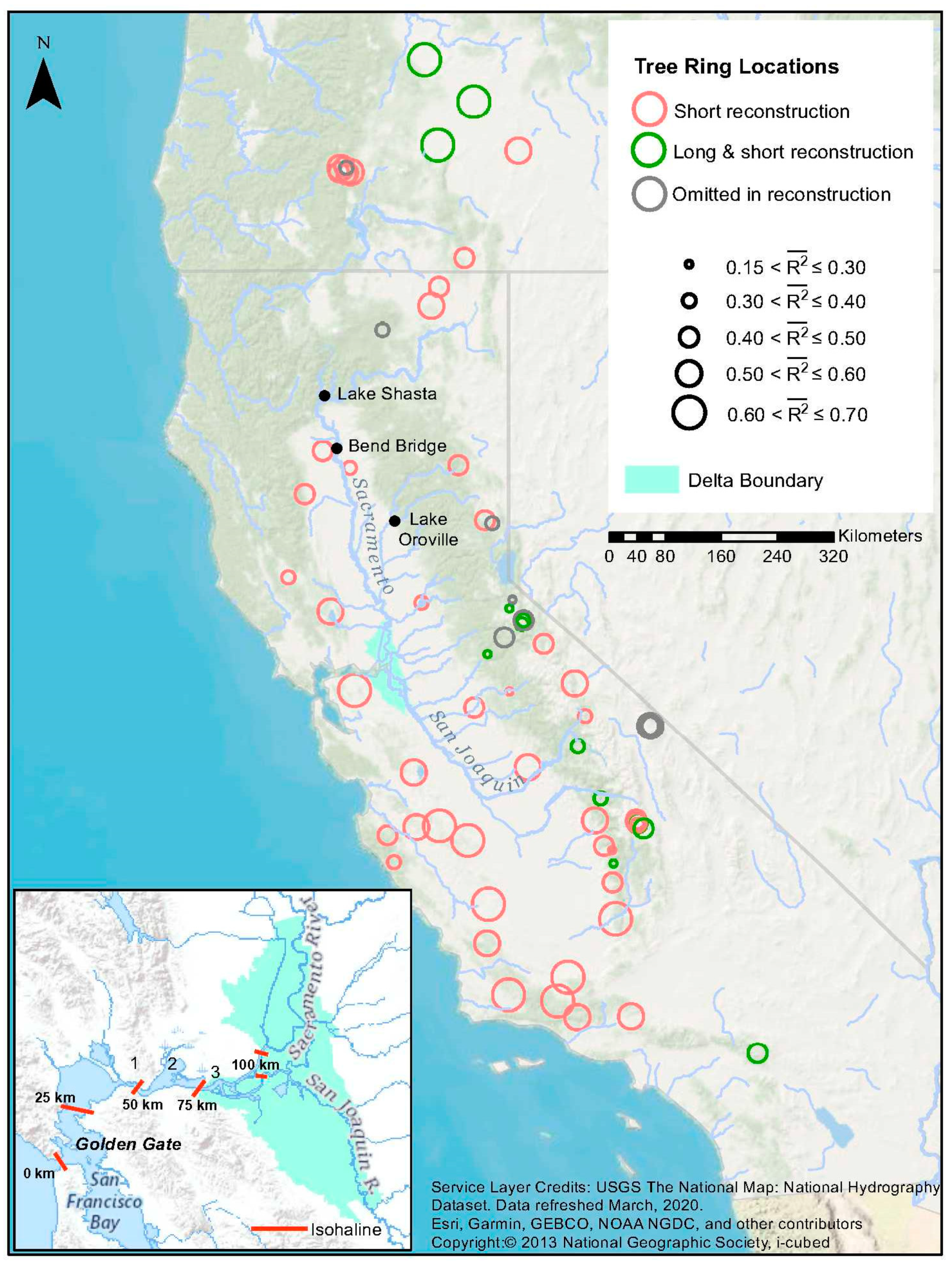
3.1.3. Tree-Ring Data

Sixty-nine tree-ring site chronologies of total ring width were assembled as part of our work (Figure 1). Each chronology typically represents many (e.g., 15 or more) trees at a specific location. Initial screening criteria were a minimum time coverage of the period 1636–2003, and geographical location within a box delineated by latitudes 34.5 N to 44.0 N and longitudes 118 W to 125 W.

We started with files of measured ring widths obtained from two studies conducted for CDWR [20,85] and supplemented those with additional files from the International Tree-ring Data Bank [86]. Ring widths were standardized uniformly into site chronologies using Matlab functions following similar protocol to that in the ARSTAN standardization package [87]. This includes fitting ring-width series with a cubic smoothing spline [88], computing core indices as the ratio of ring-width to the smooth spline and averaging the indices over cores to get the site chronology. Trend in variance indistinguishable from age or size effects was removed using the method recommended by [89]. From an assessment of the persistence in the standard chronologies and the annual flows, we decided to use the residual version [90] of the site chronologies in the reconstruction modeling. The residual chronology is an average over core indices whose low-order autocorrelation has been removed fitting the index to an autoregressive (AR) model. We used a modified Akaike information criterion [91] to select the AR order. Site chronologies are averages over fewer and fewer trees toward the early part of the tree-ring record. Adequacy of sample size for each chronology was assessed by the expressed population signal [92]. Secondary screening eliminated any site chronology whose Pearson correlation with annual flows over the available period of data overlap (subset of the WYs 1906–2018 period) was either statistically insignificant or unstable over time at significance level α = 0.05. The temporal stability of correlation was tested using a difference-of-correlation test [93] of the null hypothesis that the sample correlations for the first and second halves of the overlap are from the same population.

Additional tree-ring data and processing information are included in the Supplementary Materials section. Sites and metadata are listed in Supplementary Material A. Chronology development is described in more detail in Supplementary Material B. Additional electronic data files are also included Supplementary Materials and identified in Supplementary Material A: files of original tree-ring width measurements; a time series matrix of the residual site chronologies; a time series matrix of observed and reconstructed flows, with confidence intervals on the reconstruction.

3.2. Modeling Approach

A composite modeling approach was employed to reconstruct time series of annually varying Central Valley runoff, Delta outflow and salinity spanning more than 1000 years. The modeling approach, as summarized below, consists of three components. The purpose of the first component is to reconstruct a runoff time series from measured tree-ring data. The purpose of the second and third components is to reconstruct time series of Delta outflow and salinity from the modeled runoff time series representing the pre-development and contemporary periods, respectively. The three model components draw from a variety of measured and synthetic (i.e., simulated) calibration data. The model components and time periods are summarized in

Table 2. Summary of modeled time periods and key variables.

Time Period	WYs	Central Valley Runoff (Eight River Index)	Delta Outflow	X2 Position (Salinity)
Predevelopment	Prior to 1850	Predicted from tree-ring data using Model 1	Predicted from Equation (2) using runoff estimates and parameters in Table 5 (Model 2)	Predicted from Delta outflow using Equation (3) and parameters in Table 7 (Model 2)
Early development	1851–1911	Predicted from tree-ring data using Model 1	Predicted from Equation (2) using runoff estimates and parameters in Table 5 for pre-development period (Model 2)	Predicted from Delta outflow using Equation (3) and parameters in Table 7 for pre-developmentperiod (Model 2)
Contemporary	Post 1912	Predicted from tree-ring data using Model 1	Predicted from Equations (2) and (4) using runoff estimates and parameters in Tables 5 and 6 (Model 3)	Predicted from Delta outflow using Equation (3) and parameters in Table 7 (Model 3)

.

3.2.1. Selection of Modeled Time Periods

Our modeling approach differentiates between three eras described earlier: a “pre-development” period, an “instrumented” or “contemporary” period, and an “early development” period that bridges the pre-development and instrumented periods. Tree-ring reconstructions of Central Valley runoff were developed spanning the three time periods. A “long record” reconstruction represents the pre-development period back to WY 903 and a “short record” reconstruction represents the pre-development period back to WY 1640. Both runoff reconstructions cover the early development period spanning WYs 1851–1911; however, a unique Delta outflow and salinity model component was not generated for this period. While some literature is available to characterize the hydrology of this early development period [65,66,67,68], associated Delta outflow trends and drivers of change are poorly understood. In light of this uncertainty, we assumed that the early development period was adequately represented by pre-development relationships between runoff, Delta outflow and salinity.

3.2.2. Model 1: Annual Central Valley Runoff Reconstruction from Tree-Ring Data

Separate models were developed to reconstruct 8RI annual flows over the periods 903–2008 (long record) and 1640–2001 (short record). The long record prioritizes reconstruction length by making use of a small set of long tree-ring chronologies. The short record prioritizes reconstruction accuracy by taking advantage of a larger number of chronologies that, while not of great age, yield improved reconstruction accuracy and several centuries extension of flow beyond the gage record. The procedure described below was repeated for each of the two model periods.

A two-stage reconstruction method, introduced for reconstruction of river basin precipitation [94], and later extended for reconstruction of streamflow [53,95] was modified for this study. The first stage is conversion, by regression, of each of the available N chronologies into a separate single-site reconstruction (SSR) of y_t, the square-root-transformed annual 8RI flows. A square root transform was found adequate to correct problems with violation of assumptions about the regression residuals that occur when using the untransformed flows as the regression predictand in the reconstruction models. The second stage, called multi-site reconstruction (MSR) combines the signals from the individual SSRs to get the final single time series of reconstructed flows. The two stages of reconstruction are outlined below and are described in more detail in Supplementary Material B.

In the first stage, y_t is regressed stepwise on a pool of potential predictors that includes a site chronology, x_t, its square, $x_t^2$, and lags t − 2 to t + 2 on those two variables [96]. Preliminary stepwise modeling using cross-validation [97] is first applied to identify the step, m, beyond which addition of another predictor fails to increase the validation skill as measured by the reduction of error statistic (RE) [98]. The final SSR regression model has only those predictors entered in the first m steps, and substitution of the full available length of tree-ring predictors into the fitted equation gives the SSR reconstruction. Calibration accuracy of the SSR model is summarized by regression R². Significance of the regression model is assessed by p_F, the p-value of the overall-F of regression, and calibration uncertainty is summarized by the standard error of the estimate, or root-mean-square error (RMSE_c) of calibration [96]. Validation accuracy is summarized by the root-mean-square error of cross-validation (RMSE_v) which is computed from the cross-validation errors (see Supplementary Material B).

The product of the first stage of reconstruction in this study is a separate SSR, ${\widehat{y}}_{t,i}$, of transformed flow for each of the $i=1,\dots ,N$ tree-ring chronologies (N = 69) mapped in Figure 1. Those whose SSR calibration signal is not significant (p_F > 0.05) or whose SSR has no skill of validation (RE ≤ 0) were eliminated from the study. Depending on the time coverage (varies over SSRs), the remaining SSRs could contribute in the second stage of reconstruction.

The second stage is a re-calibration of the arithmetic mean of a subset of the N individual SSRs with acceptably strong signal and common time coverage into a final reconstruction—long or short, depending on the particular subset. The regression model for the MSR is

$$y=a+b{x}_t+e_t,$$

(1)

where x_t is the arithmetic average of the SSRs covering either the long or short records, y_t is the square-root-transformed 8RI WY flow, e_t is the error term, and $\left\{a,b\right\}$ are regression coefficients. The arithmetic average of the SSRs was preferred as a predictor with the assumption that the flow signal is best represented by the common variation in the SSRs. Since, by definition, the SSRs have variance proportional to the strength of their flow signals, a simple arithmetic average emphasizes chronologies with a strong flow signal. Equation (1) applies to both the long and short reconstructions, but for each x_t is an average over a different set of SSRs. The calibration period is defined by the overlap of 8RI flows (and y_t) with the particular SSR subset: WYs 1906–2008 for the long record and WYs 1906–2001 for the short record. Calibration and validation accuracy for the MSR models were measured by the same statistics already described for the SSR models. Substitution of the full-length SSRs into the fitted equations gave long and short reconstructions covering 903–2008 and 1640–2001, respectively. The RMSE_v of the model was used, along with the assumption that the reconstruction residuals are normally distributed, to place a 50% confidence interval on the annual reconstructed transformed flows, ${\widehat{y}}_t$. As a final step, the MSR reconstructions were back-transformed to original flow units (BCM) before interpretation.

As additional validation, time series plots and the Spearman correlation coefficient [99] were used to check agreement of the long and short reconstructions of 8RI flows spanning WYs 1872–1900 and reported in Bulletin 5 [65]. This step serves as a completely independent verification, as the Bulletin 5 data precede the start of the period used for screening tree-ring data and calibrating and cross-validating the reconstruction models. Supplementary Material C provides the statistics of the SSR models.

Low-frequency features (decadal and longer) are of interest in understanding long-term hydrologic patterns. Severity of droughts and wet periods is also summarized by simple moving averages of reconstructed flows. Consistency of with other work was checked by comparing reconstructions with the sum of separate reconstructions of annual Sacramento River and San Joaquin River flow [20].

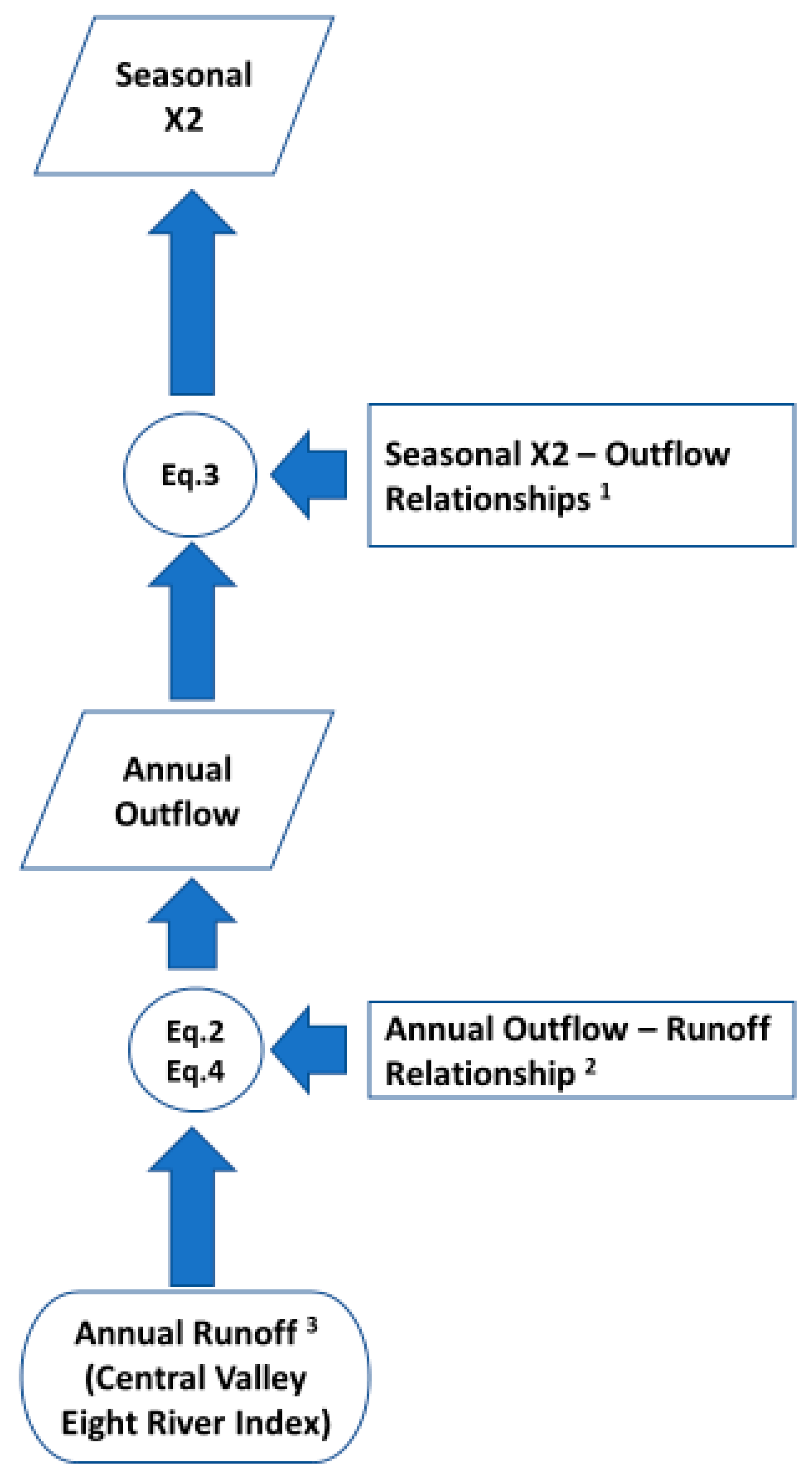
3.2.3. Model 2: Pre-Development Outflow and Salinity Reconstruction

The annual 8RI time series tree-ring reconstructions from Model 1 were used as the basis for reconstructing annual Delta outflow volume and salinity in the estuary under pre-development conditions. The modeling logic employed for the long- and short-period reconstructions is presented as a flow chart in Figure 2.

Annual pre-development Delta outflow volume was estimated for both reconstruction periods assuming a power law relationship between Delta outflow volume and annual Central Valley runoff volume:

$$Delta Outflow={\mathsf{\alpha }}_1\times 8{\mathrm{RI}}^{{\mathsf{\alpha }}_2}$$

(2)

where outflow and runoff volumes are in units of BCM per year and α₁ and α₂ are fitting parameters determined through least squares analysis [25] simulated pre-development conditions in the Central Valley and Delta assuming a historical runoff pattern measured over the 93-year period spanning WYs 1922–2014. Annual Delta outflow volume from the CDWR simulation, along with annual Central Valley runoff (as measured by the 8RI over the same 93-year period), were used to calibrate Equation (2). Tree-ring reconstructions of Central Valley runoff (i.e., the 8RI) were used in conjunction with Equation (2) to estimate pre-development annual Delta outflow volumes through WY 1850.

Seasonal (February–June and July–October) average pre-development X2 positions were estimated for the reconstruction periods assuming power law relationships between X2 position and annual Delta outflow volume:

$$\mathrm{X}2={\mathsf{\alpha }}_3\times Delta Outflo{w}^{{\mathsf{\alpha }}_4}$$

(3)

where X2 position is in units of km from Golden Gate and α₃ and α₄ are fitting parameters determined through least squares analysis. The 93-year simulated pre-development Delta outflow time series, as described above, was utilized to calibrate Equation (3). Several modeling steps were followed to generate 93-year X2 calibration data sets. First, daily outflow from the aforementioned CDWR [25] simulation was transformed into a daily “antecedent outflow” time series to represent flow time-history in the estuary [14,84]. This transformed outflow time series was used to generate a daily X2 time series using a pre-development flow–salinity relationship reported by [26]. Finally, this synthetic daily X2 time series was averaged to develop seasonal average X2 calibration time series. Time series of annual pre-development outflow volume, estimated from the tree-ring reconstructions (Model 1), were used in conjunction with Equation (3) to estimate seasonal average X2 positions through WY 1850.

3.2.4. Model 3: Contemporary Outflow and Salinity Reconstruction

Following the methods reported above for pre-development conditions, the annual 8RI time series tree-ring reconstructions from Model 1 were used as the basis for reconstructing annual Delta outflow volume and salinity in the estuary under contemporary conditions. The modeling logic employed for the reconstructions is presented as a flow chart in Figure 2. This logic was applied to both the long- and short-period reconstructions spanning WYs 1912–2008 and WYs 1912–2001, respectively.

Contemporary Delta outflow was estimated for both reconstruction periods assuming the power law relationship provided in (Equation (2)). This relationship, which was calibrated with historical annual runoff and Delta outflow data, does not represent the full contemporary period; rather, it is limited to a relatively stationary period prior to significant increases in water use in the Central Valley and Delta following construction of Shasta Dam in WY 1944. A residual analysis was conducted to address the observed time series trend. Tree-ring reconstructions of Central Valley runoff (from Model 1) were used in conjunction with Equation (2) to estimate contemporary annual Delta outflow volumes for the WYs 1912–1944 period; a modified form of Equation (2), presented later in this text, was used to estimate Delta outflow volumes for the post 1944 period.

Contemporary X2 position was estimated for the long- and short-period reconstruction periods assuming power law relationships between annual Delta outflow volume and seasonal (February–June and July–October) average X2 position. Equation (3) was calibrated for the contemporary period using a data subset spanning WYs 1920–2018. The initial years of the contemporary period (WYs 1912–1919) were excluded from model calibration due to lack of historical Delta outflow data at a daily resolution. Following the methodology used for pre-development model calibration, daily outflow was transformed into a daily antecedent outflow time series and this daily antecedent outflow time series was then transformed into a daily X2 time series using a contemporary flow–salinity relationship reported by Andrews et al. [26]. Finally, this daily X2 time series was averaged to develop seasonal average X2 time series for purposes of model calibration. The time series of annual contemporary outflow volume, estimated from the tree-ring reconstructions, were then used in conjunction with Equation (3) to estimate seasonal average X2 positions for each time series beginning in WY 1912.

4. Results

Following the methods presented in the previous section, we developed multi-century reconstructions of watershed runoff, freshwater flows to the estuary, and the estuary’s salinity regime as expressed by intrusion length. Below we summarize the reconstructions, following the logic sequence provided in the flow chart depicted in Figure 2.

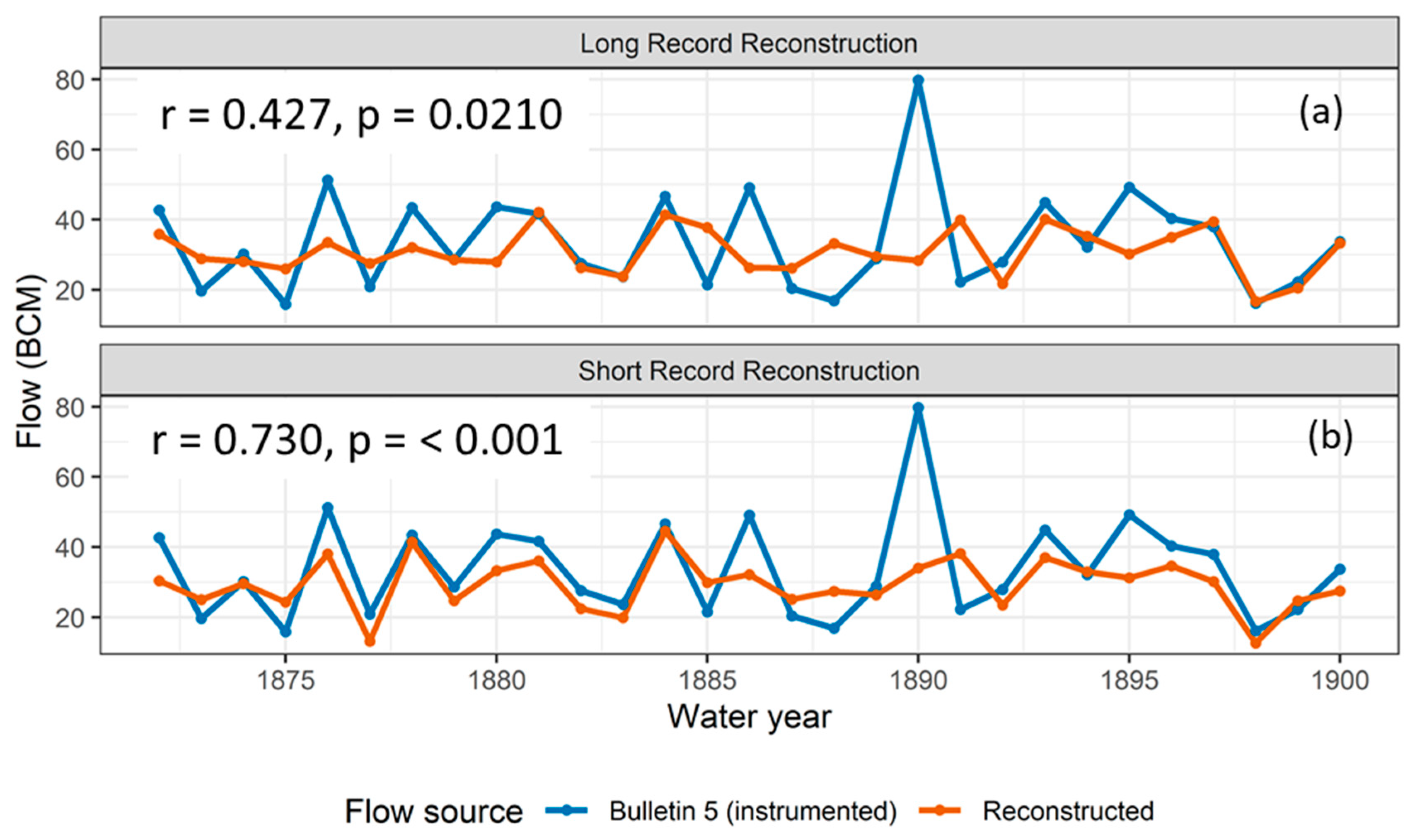
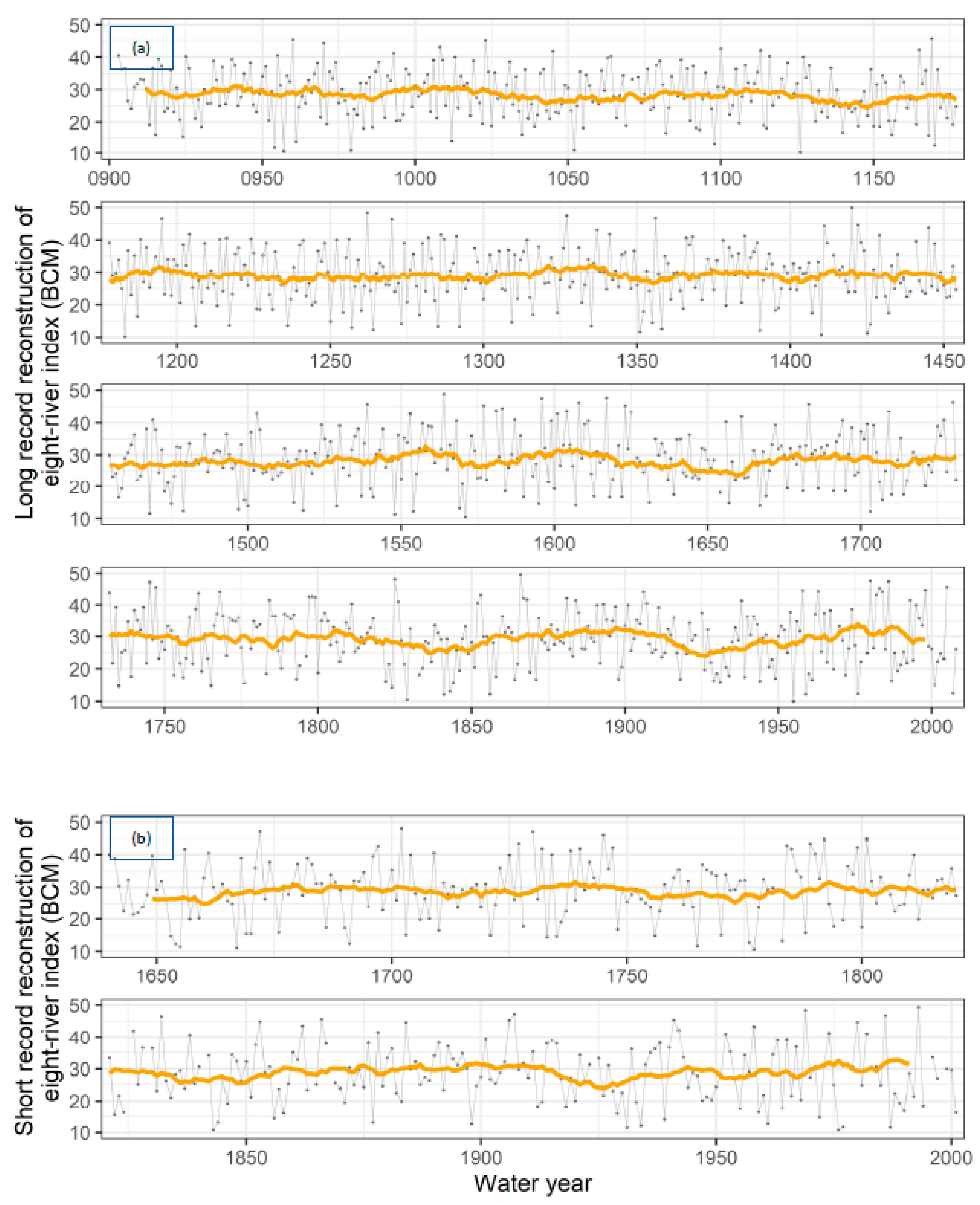
4.1. Annual Central Valley Runoff Reconstructions

A total of 60 of the 69 initial chronologies passed screening tests for temporal stability of the runoff signal and significant SSR regression model (Supplementary Material C). Most of these lagged models resulting from stepwise regression have a simple structure. All 60 models include a lag-0 (current year predictor) and 28 models have just one predictor. The median number of predictors is 2 and the maximum is 5. The minimum, median and maximum percentage of calibration-period variance explained by the models are 8%, 29% and 73%, respectively. All models are significant as judged by p < 0.05 for the overall F of regression. Blue oak chronologies from the Central Valley or the coastal region tend to have the strongest signal (Figure 1).

Time coverage by SSRs varies according to the coverage of the chronologies themselves. Thirteen of the SSRs have uniform coverage for 903–2008 and comprise the subset for the long reconstruction; all 60 SSRs, with a common period 1640–2001, are available for the short reconstruction. As in previous studies (e.g., Meko et al. [53]), long tree-ring chronologies of western juniper from south-central Oregon are important contributors to the long network (Figure 1).

Regression of y_t on the 13-site-mean and 60-site-mean SSRs yields long and short reconstruction models accounting for 66% and 77% of the calibration-period variance of y_t after adjustment for loss of degrees of freedom (adjusted R²) (

Table 3. Statistics for long record and short record tree-ring reconstructions (Model 1). Statistics are for regression models whose predictand is transformed 8RI flow (square root billion cubic meters).

Tree-Ring Record	Na	Calibration b			Cross-Validation c
		WYs	R2 adj	RMSE	RMSE	RE	r
Long record 903–2008	13	1906–2008	0.66	0.697	0.712	0.65	0.82
Short record 1640–2001	60	1906–2001	0.77	0.585	0.592	0.77	0.88

^a Number of contributing tree-ring chronologies. ^b Overall F (not listed) for both models is highly significant (p < 1E-25). ^c RE = reduction-of-error statistic; r = correlation of cross-validation predictions with observed flows. The two correlations listed are both larger than any of the correlations for the 1000 simulated reconstructed flow series (p < 0.001)

). Both models have strong validation, as indicated by high positive RE values from cross-validation, and by highly significant correlation of cross-validation predictions with observed flow. Both reconstructions also closely track and have significant correlation with earlier flows (spanning WYs 1872–1900) from gages on the Sacramento, San Joaquin, and other Central Valley rivers that comprise the Bulletin 5 8RI flows (Figure 3) [65]; these earlier data had also been used, with less success, for validation of the first Sacramento River runoff reconstruction [51]. Both models greatly underestimate the flow in WY 1890. Tree-ring reconstruction calibrated by regression with gaged flows tend to be conservative (biased toward the mean) because the variance explained by regression is always less than 100%. This compression of variance theoretically would lead to underestimation of both wet extremes and dry extremes and complicates direct comparison of observed and reconstructed magnitudes of extreme flow events [83]. Moreover, as seen in Figure 3, the magnitude of extreme high flows may be especially difficult to capture because growth of drought-sensitive trees beyond some high level of soil moisture is logically expected to benefit less and less from additional moisture.

Both the short and long record reconstructions strongly track the sum of individual reconstructions generated previously for the Sacramento and San Joaquin Rivers by Meko et al. [20]. For the 1640–2001 period common to these reconstructions, the Pearson correlation is r = 0.83 for the long record reconstruction and r = 0.95 for the short record reconstruction. For the earlier 903–1639 period in common with the long reconstruction only, the correlation remains high (r = 0.82). While agreement between reconstructions is limited by differences in tree-ring networks and statistical reconstruction methods, the reconstructions are reasonably consistent in their characterization of droughts and wet periods. The long record reconstruction, for example, includes a period of low runoff values in the mid-1100s that aligns with a period of notable persistent drought in both the Colorado and Sacramento Basins [95,100].

The long and short record 8RI reconstructions are shown in Figure 4, indicating annual and 5-, 10-, 20-, and 100-year center-averaged values. When the late-19th to early 20th century reconstructed flows are compared with reconstructed flows in the preceding centuries, it is apparent that single-year wet and dry extremes are more variable, however, time averaged flows are more consistent over the different periods. This is also summarized in

Table 4. Range of reconstructed and instrumented Central Valley Runoff (8RI) for different averaging periods. Units are reported as BCM.

8RI Record	WYs	Center Averaging Period (yr)	Min	Max	Range	5%	10%	25%	50%	75%	90%	95%
Long Record Reconstruction	903–2008	5	16.6	41.4	24.7	23.0	24.3	26.5	28.8	31.0	32.7	33.9
Short Record Reconstruction	1640–2001	5	18.7	39.9	21.2	22.1	23.3	26.0	28.7	31.3	34.0	35.4
Long Record Re- Construction	1872–2001	5	19.5	41.4	21.8	22.0	24.4	26.7	29.7	32.3	34.6	36.3
Short Record Re- Construction	1872–2001	5	19.7	39.9	20.1	22.3	23.4	26.3	29.5	31.9	35.3	37.0
Instrumented Flows	1872–2018	5	16.0	44.5	28.5	19.1	22.3	25.4	31.2	34.5	39.0	41.4
Long Record Re- Construction	903–2008	10	21.3	38.2	16.9	24.8	25.7	27.2	28.7	30.2	31.6	32.4
Short Record Re- Construction	1640–2001	10	21.9	36.3	14.3	24.3	25.3	27.2	28.8	30.4	32.3	33.1
Long Record Re- Construction	1872–2001	10	21.3	38.2	16.8	23.0	25.6	27.4	30.1	31.5	32.7	34.1
Short Record Re- Construction	1872–2001	10	21.9	36.2	14.3	24.1	25.7	27.4	29.4	31.1	32.9	33.4
Instrumented Flows	1872–2018	10	20.2	40.3	20.2	21.7	23.9	27.2	31.1	33.8	36.3	37.5
Long Record Re- Construction	903–2008	20	23.7	33.9	10.2	25.9	26.6	27.6	28.7	29.8	30.7	31.3
Short Record Re- Construction	1640–2001	20	24.1	32.6	8.55	25.9	26.6	27.7	29.0	30.0	30.7	31.2
Long Record Re- Construction	1872–2001	20	23.9	33.9	9.94	25.0	25.7	27.4	30.2	31.4	32.3	32.7
Short Record Re- Construction	1872–2001	20	24.1	32.6	8.55	25.3	26.3	27.9	29.5	30.6	31.3	31.8
Instrumented Flows	1872–2018	20	22.4	38.4	16.0	24.7	25.8	28.1	29.9	33.8	35.4	36.2
Long Record Re- Construction	903–2008	100	27.2	29.8	2.58	27.6	27.8	28.1	28.7	29.1	29.3	29.4
Short Record Re- Construction	1640–2001	100	27.9	29.4	1.50	28.2	28.4	28.6	28.8	29.0	29.2	29.2
Long Record Re- Construction	1872–2001	100	28.8	29.5	0.734	28.9	29.0	29.0	29.1	29.3	29.4	29.4
Short Record Re- Construction	1872–2001	100	28.6	29.4	0.763	28.7	28.7	28.8	28.9	29.1	29.3	29.4
Instrumented Flows	1872–2018	100	28.0	31.2	3.20	28.4	28.6	29.4	29.9	30.7	30.9	31.0

, which shows that for all of the averaging periods presented, from 5 to 100 years, the range of flows are essentially similar for the full reconstruction and the more recent 1872–2001 period. Importantly, the entirety of the instrumented period, 1872–2018, generally shows a wider range in flows that the reconstructed values. Additionally, low flows over different averaging periods are lower in the instrumental record than in the longer reconstruction period. This comparison suggests that the instrumental flow record is a reasonable representation of the conditions over the past millennium and captures extremes in the low flow periods.

Another way to look at the flow reconstructions is to examine the sequence of wet and dry periods in the record, in comparison to the contemporary period. The long record reconstruction was reviewed to highlight patterns of low and high flows that are of interest for water resources management. Figure 5 shows 20-year center averages associated with four 121-year periods with the greatest variations (970–1090; 1100–1220; 1570–1690; 1850–1970). This figure illustrates that shifts between wet and dry periods have occurred several times in the past millennium, but in most of these instances, the range of flow variation is not greater than the reconstructed flows for late 19th and early 20th century. Actual observed flows during high flow periods are higher that the reconstructed flows, a bias expected from the variance compression inherent in regression, and possibly also to lower sensitivity of tree-growth to soil moisture beyond a threshold level. However, if only reconstructed flows are considered for comparison over different time periods, as done throughout this study, it may be inferred that flow patterns in the instrumental period after the 1870s, especially over decadal time scales, are a reasonable representation of the overall variability seen in the past millennium.

4.2. Delta Outflow: Model Calibration and Reconstructions

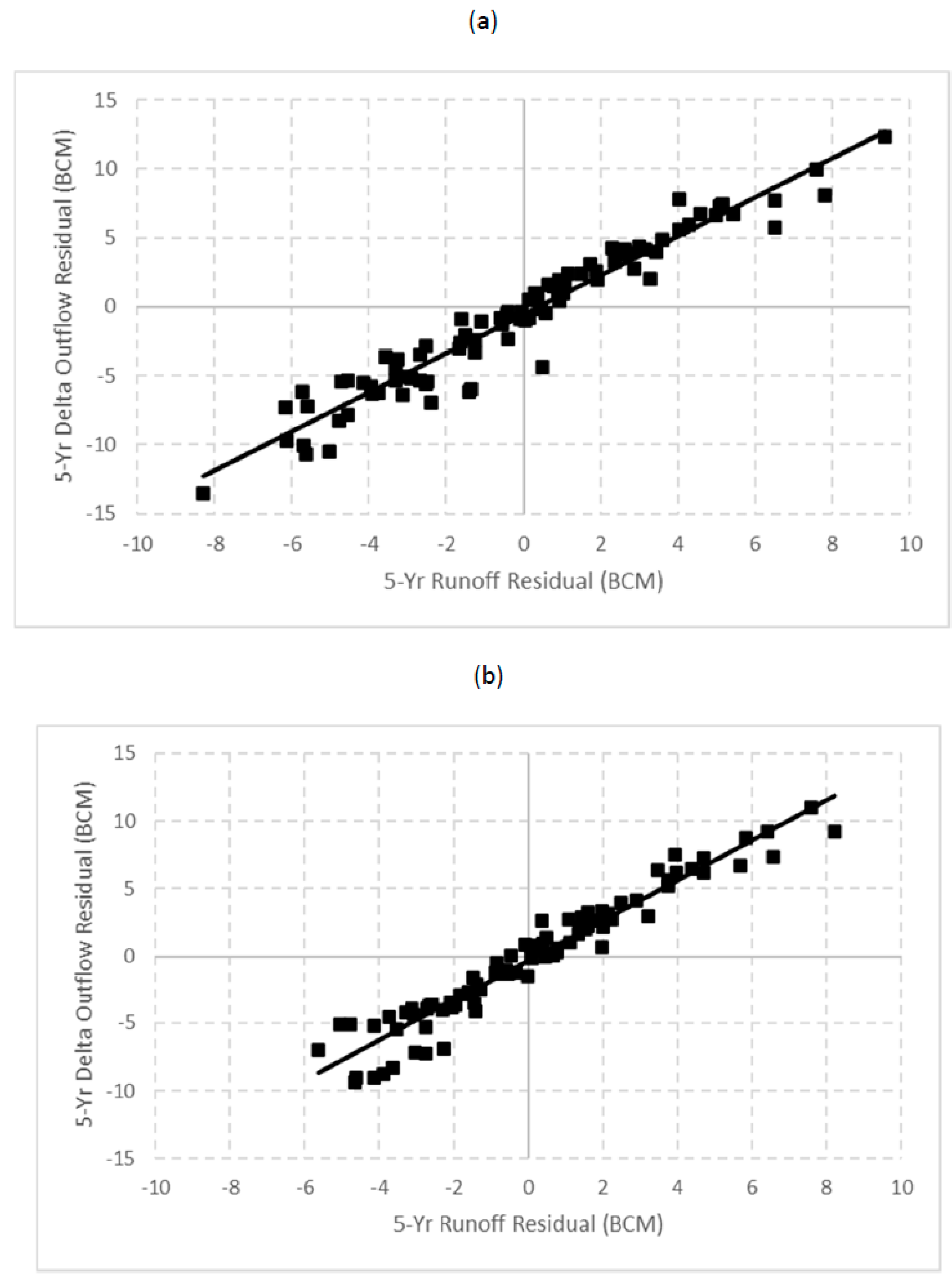
4.2.1. Model Calibration

The resulting pre-development relationship between Delta outflow and Central Valley runoff, both expressed in terms of annual flows, is displayed in Figure 6. Equation (2) fitting parameters and regression statistics are summarized in

Table 5. Model fitting parameters and regression statistics for Equation (2): relationships between Delta outflow and Central Valley runoff under pre-development (Model 2) and contemporary (Model 3) conditions. Flow units are in BCM per year.

Model	α1	α2	r2	Std. Error (BCM)
Pre-development (Model 2)	0.380	1.23	0.956	2.7
Contemporary WYs 1912–1944 (Model 3)	0.285	1.38	0.991	1.5
Contemporary WYs 1945–2018 (Model 3)	(1)	(1)	(1)	(1)

⁽¹⁾ The contemporary outflow–runoff relationship for WYs 1945–2018 was adjusted using Equation (4) to reflect significant increases in water use in the Central Valley and Delta following construction of Shasta Dam in WY 1944. See Table 6.

.

Historical annual Delta outflow was correlated with annual Central Valley runoff (as measured by the 8RI) over a subset of the contemporary period spanning WYs 1912–1944; the resulting model fit is displayed in Supplementary Material D (see Figure D-1). Equation (2) fitting parameters and regression statistics are summarized in Table 5. Model residuals, reported as predicted minus observed, are plotted as a time series in Figure 7a for the full contemporary period spanning WYs 1912–2018. This figure clearly shows that Equation (2) increasingly over-estimates Delta outflow over time following WY 1944, signifying a decreasing trend in Delta outflow relative to the 8RI. Equation (2) residuals were de-trended through the following re-formulation (see Figure D-2 in Supplementary Material D):

$$Delta Outflow={\alpha }_1\times 8{\mathrm{RI}}^{{\mathsf{\alpha }}_2}\times \left\{1-\left[{\mathsf{\alpha }}_8\times {\left(Water Yr-1944\right)}^2+{\mathsf{\alpha }}_9\times \left(Water Yr-1944\right)+{\mathsf{\alpha }}_{10}\right]\right\}$$

(4)

where α₈, α₉, and α₁₀ are dimensionless fitting parameters. Hutton et al. [101] observed that Delta outflow trends, when normalized to the 8RI, were different between low and high runoff years. In high runoff years, they observed a decreasing trend in normalized outflow. However, they reported that:

In drier years, the downward trend in normalized Delta outflow appears to have been curbed (and possibly reversed) over the last few decades due to more restrictive water management (i.e., lower normalized Delta exports) in the estuary and a leveling of water use in the upstream watershed.

Following the observations of [101], Equation (4) was independently calibrated for low runoff years (8RI < 24.6 BCM/yr) and high runoff years (8RI > 24.6 BCM/yr) with a combined standard error of 3.0 BCM. Fitting parameters and regression statistics are provided in

Table 6. Model fitting parameters and regression statistics for Equation (4): adjusted relationships between Delta outflow and Central Valley runoff under WYs 1945–2018 contemporary (Model 3) conditions.

Fitting Parameter/ Regression Statistic	Low Runoff Years 8RI < 24.6 BCM/yr	High Runoff Years 8RI > 24.6 BCM/yr
α1	0.285	0.285
α2	1.38	1.38
α8	−0.000137	0
α9	0.0148	0.00426
α10	0	0.0863
R2	0.474	0.482

. Model residuals, reported as predicted minus observed, are plotted as a time series in Figure 7b. This figure shows no apparent time trend in the de-trended model residuals. The tree-ring reconstructions of Central Valley runoff (i.e., the 8RI) were used in conjunction with Equations (2) and (4) to estimate contemporary annual Delta outflow volumes for each time series beginning in WY 1912.

4.2.2. Delta Outflow Reconstructions

The annual Central Valley runoff reconstructions (long record and short record) were used as the basis for reconstructing Delta outflow volume under pre-development and contemporary conditions using Models 2 and 3 described above. The results are shown in the form of exceedance frequencies in Figure 8. Through WY 1850, the plot shows little difference between the long and short record reconstructions to estimate pre-development annual Delta outflow volumes. Annual outflow volumes for this period are approximately 35–37 BCM, 24 BCM and 11–13 BCM at the 10th, 50th and 90th percentiles, respectively. For the contemporary period beginning in WY 1912, the plot shows small differences between the long and short record reconstructions. Annual outflow volumes for this period are approximately 40–44 BCM, 24 BCM and 9–11 BCM at the 10th, 50th and 90th percentiles, respectively.

Differences between pre-development and contemporary Delta outflow conditions reflect differences observed in the Central Valley runoff reconstructions as well as differences in water use on the valley floor and in the Delta. For example, assuming a common historical runoff sequence from WYs 1922–2003, Gross et al. [22] reported mean annual Delta outflows of 24.5 BCM and 19.4 BCM under pre-development and contemporary conditions, with the difference approximately equal to CVP and SWP exports from the south Delta, which together average approximately 6.1 BCM [22]. Our work shows similar mean annual Delta outflow conditions (24 BCM) for the pre-development and contemporary periods. However, the contemporary period is associated with a more variable outflow regime relative to the pre-development period, with higher outflows in the low end of the exceedance frequency domain and lower outflows in the high end of the exceedance frequency domain.

Contemporary outflow model residuals associated with Equations (2) and (4) are highly correlated (R² = 0.94) with reconstructed Central Valley runoff residuals. Residuals are computed as the difference between reconstructed values and historical values. Figure 9 shows scatter plots and regression lines for long record (WYs 1912–2008) and short record (WYs 1912–2001) relationships, with residuals shown as 5-year center weighted averages.

4.3. X2: Model Calibration and Reconstructions

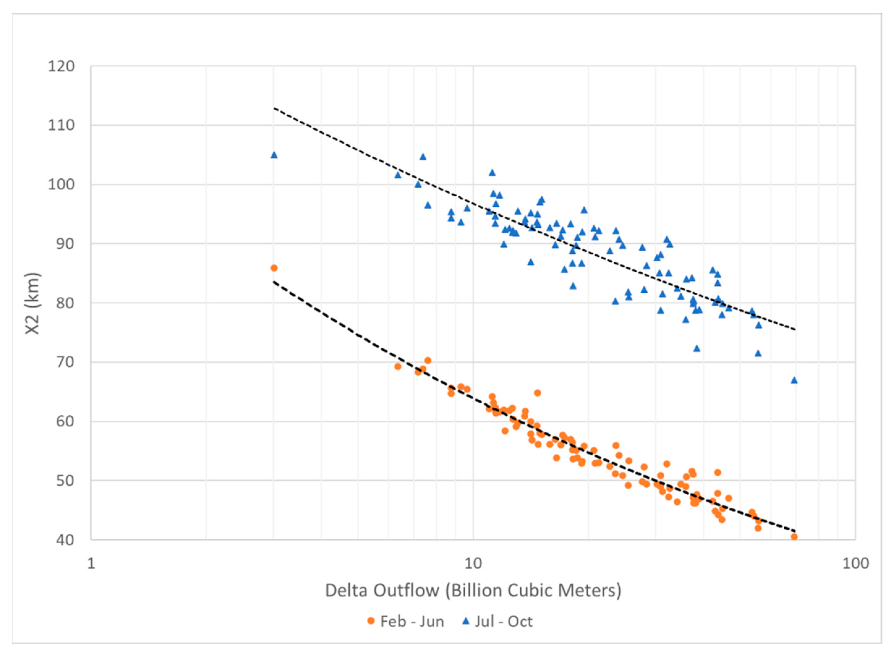
4.3.1. Model Calibration

The resulting pre-development relationships between seasonal average X2 and annual average Delta outflow are displayed in Figure 10. Equation (3) fitting parameters and regression statistics are summarized in

Table 7. Model fitting parameters and regression statistics for Equation (3): relationships between X2 position and Delta outflow under pre-development (Model 2) and contemporary (Model 3) conditions X2 is in units of km from Golden Gate and outflow units are in BCM per year.

Model	Season	α3	α4	r2	Std. Error (km)
Pre-development (Model 2)	February–June	107	−0.223	0.943	1.7
Pre-development (Model 2)	July–October	130	−0.128	0.763	3.7
Contemporary WYs 1912–1944 (Model 3)	February–June	120	−0.242	0.974	1.5
Contemporary WYs 1912–1944 (Model 3)	July–October	142	−0.137	0.760	4.8
Contemporary WYs 1945–2018 (Model 3)	February–June	122	−0.228	0.886	3.6
Contemporary WYs 1945–2018 (Model 3)	July–October	113	−0.106	0.709	4.0

. Step changes in contemporary relationships between annual Delta outflow volume and seasonal average X2 position were observed following construction of Shasta Dam in 1944. Hutton et al. [101] observed statistically significant trends in seasonal outflows, with decreasing trends observed in four months (February, April, May and November) and increasing trends observed in two months (July and August). The authors discussed linkages between outflow trends and changes in upstream flows and coincident developments such as reservoir construction and operation, out-of-basin imports and exports, and expansion of irrigated agriculture. The resulting contemporary pre- and post-WY 1945 relationships between seasonal average X2 and annual Delta outflow volume are shown in Supplementary Material D (Figures D-3 and D-4) and regression statistics are summarized in Table 7. Although a physical basis exists for developing independent correlations for the pre- and post-1945 February–June relationships, we note that the derived fitting parameters are not statistically different from one another.

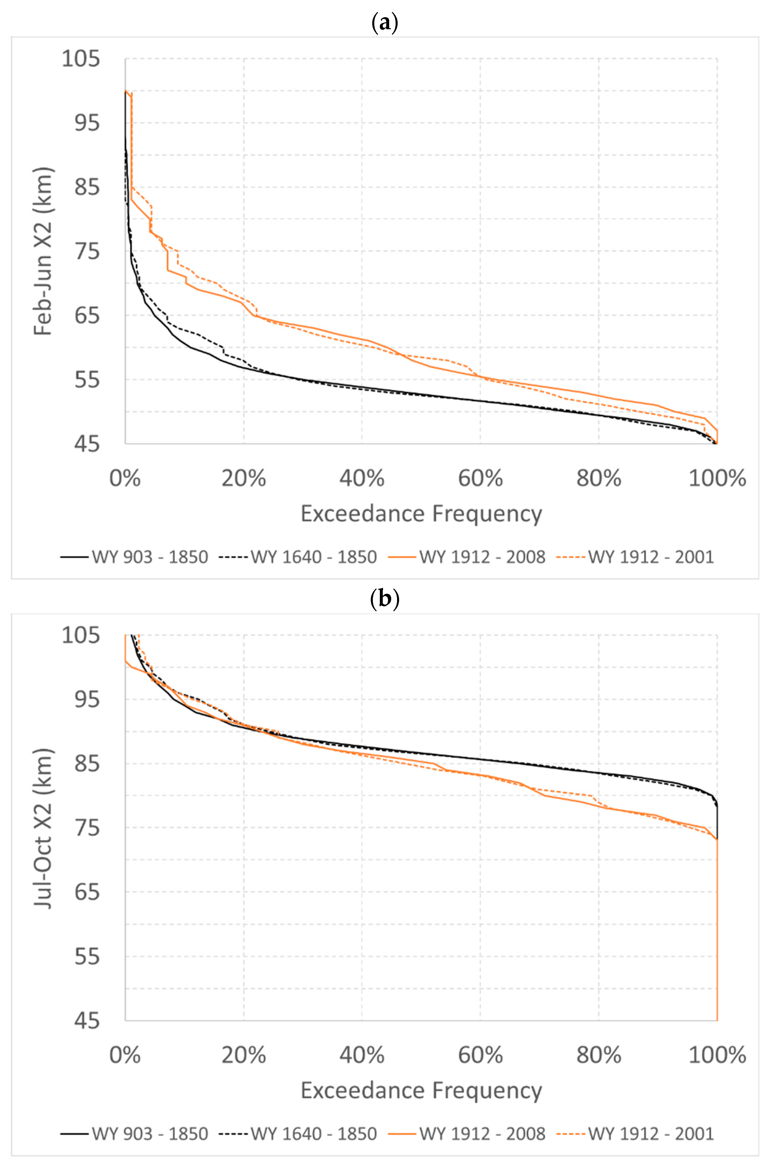
4.3.2. X2 Reconstructions

The annual Delta outflow reconstructions (long record and short record) were used as the basis for reconstructing seasonal (February–June and July–October) average X2 position under pre-development and contemporary conditions, using Models 2 and 3 described above. Figure 11 shows pre-development seasonal average X2 exceedance frequencies for each reconstruction. Little difference is observed between the pre-development long and short period reconstructions except in the 10th–20th percentile range. As shown in the top panel, February–June average X2 positions are approximately 60–63, 53 and 48 km at the 10th, 50th and 90th percentiles, respectively. X2 is further downstream (smaller values) in the spring, indicative of relatively higher flow conditions. As shown in the bottom panel, July–October average X2 positions are approximately 94–96, 86–87 and 82–83 km at the 10th, 50th and 90th percentiles, respectively. X2 is further upstream (larger values) in the summer and fall, indicative of relatively lower flow conditions.

This same figure shows small differences between the reconstructions throughout the exceedance frequency domain for the contemporary period beginning in WY 1912. February–June average X2 positions are approximately 70–73, 58–59 and 50–51 km at the 10th, 50th and 90th percentiles, respectively. July–October average X2 positions are approximately 94–96, 84–86 and 76–77 km at the 10th, 50th and 90th percentiles, respectively. As under pre-development conditions, contemporary X2 is further downstream (smaller values) in the spring and further upstream (larger values) in the summer and fall.

Differences between pre-development and contemporary X2 conditions reflect differences observed in the Delta outflow reconstructions and differences in interannual pattern of water use. Differences in X2 also reflect natural and anthropogenic drivers that modified the estuary’s flow–salinity regime, resulting in greater outflow requirements under contemporary conditions to repel salinity intrusion [22,26] The contemporary period is generally associated with greater spring (February–June) salinity intrusion and lesser summer–fall (July–October) salinity intrusion relative to the pre-development period. Seasonal differences between pre-development and contemporary X2 conditions are indicative of upstream reservoir operations that store water in winter and spring months and release water in summer and fall months.

5. Discussion

Flow and salinity have been the subject of scientific observation in San Francisco Estuary over more than a century [14,65]. These observations, which have provided a reasonable understanding of contemporary conditions and associated trends in the estuary over the past century, have also supported decision-making related to freshwater flow management in the estuary. However, important knowledge gaps exist that cannot be addressed solely by the available observations. These gaps relate to the fact that large-scale changes in the estuary and its watershed pre-date the observational record by several decades; these gaps also relate to the fact that California is known to have been subject to highly variable climatic conditions over the past millennium. Additional data collection is thus insufficient to provide an understanding of how the system behaved prior to the initiation of large-scale disturbances after the mid-19th century. This work is an attempt to fill these gaps by (i) using an updated set of tree-ring chronologies to represent annual runoff into the Central Valley from the surrounding higher-elevation watersheds over the past millennium and (ii) utilizing a modeling approach to relate runoff to freshwater flow to the estuary and to salinity intrusion in the Delta. This integration of tree-ring based estimates of runoff with models of flow and salinity representing different configurations of the system (pre-development and contemporary) allows for a more nuanced exploration of flow and salinity changes over periods much longer than covered by the instrumented record. This information is of scientific and practical importance because it can help guide decisions related to the restoration of the estuarine ecosystem. These decisions have recently focused on potential changes to flow and salinity management in the estuary [18], decisions with major environmental and economic consequences for California.

The updated tree-ring-based reconstruction shows a mean annual Central Valley runoff (8RI) of approximately 29 BCM, a quantity that is similar to that observed in the contemporary system. The reconstruction also shows large single-year anomalies from the mean, although multi-year anomalies over averaging periods of 5–100 years are minimal. An important observation is that, while high runoff extremes overlap with the instrumented record, their magnitudes are lower than observed. The reconstruction indicates the occurrence of individual years with runoff significantly lower than seen in the gauged record; however, over longer averaging periods, pre-development runoff variations are of similar magnitude to those in the instrumented period and represent broadly similar patterns of wet and dry periods. Our findings are contrary to some prior reconstructions—notably Stine [47] based on the position of tree stumps at Mono Lake and Graham and Hughes [48] focused on Merced River runoff and the Mono Lake Basin inflow—that indicate evidence of more severe droughts over the past millennium than any seen in the instrumented period. However, our findings are broadly consistent with the work of Meko et al. [20] that focused on a smaller set of tree-ring data from the Sacramento and San Joaquin River basins. Our work confirms that major long-term deviations from the mean runoff in California’s Central Valley are often seen in the tree ring record, but the extended drought of the late 1920s and early 1930s compares with the most extreme in the past millennium.

Consistent with the historical pattern of flow variability, California at the end of WY 2020 appears to be in the midst of another severe long-term drought. The Eight River Index, averaged over the preceding 20-years from WY 2020, stands at 25.6 BCM; long-term average runoff of lower magnitude was last seen in the severe drought of the 1920s and 1930s, when 20-year average flows from WY 1931 to 1939 ranged from 22.4 to 25.1 BCM.

Integration of the tree-ring based runoff with downstream flow models shows that, although median freshwater flows into the estuary have not changed significantly, Delta outflow has been more variable in the contemporary period compared to pre-development conditions. Extending to salinity, the contemporary period is associated with greater spring (February–June) salinity intrusion and lesser summer–fall (July–October) salinity intrusion relative to the pre-development period. Both outflow and salinity intrusion are directly affected by contemporary reservoir storage and release patterns, which tends to smoothen the intra-annual extremes that are seen in the pre-development system.

Our work can also be compared with similar research by Stahle et al. [23] who used tree-ring chronologies to relate to salinity intrusion in the Delta. Using a 625-year (1379–2003) tree ring chronology to reconstruct the February–June average X2 position in San Francisco Estuary, the authors were able to explain 73% of the variance in the observed X2 data over a 1956–2003 calibration period. The authors used their reconstructed salinity record to examine return intervals between single-year X2 extremes and to quantify the frequency of consecutive seasonal maxima and minima over the period of record. [23] recognized that their reconstruction does not mimic pre-development salinity conditions in the estuary. Rather, the authors concede that their X2 time series:

… provides an estimate for variability in the salinity gradient on interannual-to-decadal time scales, given the present land cover, stream morphology, and regulated flow environment, in response to the range of modern and prehistoric seasonal precipitation totals registered in the tree-ring record over the past 625 years.

In other words, the authors employed a “level-of-development” methodological approach [22,24,63] and their 625-year X2 reconstruction represents salinity variability under a contemporary level of development. Stahle et al. [23] found the hydroclimatic signal from tree growth to be approximately stationary over the past six centuries; thus, we expect that their estimate would be consistent with the contemporary level X2 time series presented by Gross et al. [22] that utilized a shorter, more recent climate sequence spanning WYs 1922–2003.

In contrast with [23], our work explicitly attempts to reconstruct an extended record of historic salinity conditions in the estuary. Our work relies on modeled relationships between Central Valley runoff, Delta outflow and estuarine salinity under natural and anthropogenically altered hydrologic conditions as they occurred over the period spanning 903–2008 (long record) and 1640–2001 (short record). We expect that our pre-1850 estimates would be consistent with the pre-development level X2 time series presented by Gross et al. [22] similarly, we expect that our post-1944 estimates (following construction of Shasta Dam) would be consistent with the contemporary level X2 time series presented by [22]. Consistent with Gross et al. [22], our work shows that, in spite of a relatively stationary hydroclimatic signal from tree growth (a proxy for Central Valley runoff), the San Francisco Estuary’s seasonal salinity pattern has changed due to anthropogenic alterations. Specifically, both studies suggest that the estuary is now more saline in the late winter and spring than it was under pre-development conditions because of contemporary water management. Both studies also show that the contemporary estuary is less saline in the late summer and fall than it was under pre-development conditions because of water management.

Flows in the observed record from WY 1872 onwards display significant change, with a wet period from the late 19th century to the first decade of the 20th century, followed by a severe drought in the late 1920s and early 1930s. As noted earlier, these were drivers of the early water resources engineering activities in California, with a focus on flood control in the late 19th century to be followed by a focus on regulation and storage by the 1920s and beyond. The longer flow reconstruction in this work highlights that this period in the observed record captures the types of extreme shifts that have occurred over the past millennium. These reconstructed data therefore show that widely used level-of-development modeling approaches, that repeat the instrumental sequence of flows for different estuary and watershed configurations, appear to be an appropriate methodology for representing a range of pre-development conditions.

The agreement between the tree-ring record with the earliest hydrologic observations confirms and draws attention to a period of dramatic hydrologic change during the late 19th and early 20th centuries, a shift driven by natural factors coupled with rapid regional development. Thus, population growth and extensive watershed modification was overlaid on the underlying hydrologic shift from very wet to very dry conditions, which complicates the task of inferring estuarine changes in the early development period (WYs 1850–1911). Putting this hydrologic shift in the context of other anthropogenic drivers is important in understanding how the estuary responded during this early period and in setting salinity targets for estuarine restoration.

Although tree-ring proxies from long-lived species with high sensitivity to drought are a powerful tool for water resources planning in California, some important caveats are noteworthy. As indicated by the reconstruction statistics, tree-ring width is an imperfect proxy for Central Valley precipitation. In our work, uncertainty is greatest in the early part of the tree-ring record because the data network thins. In particular, the tree-ring record suffers from limited blue oak data, a tree which is shorter-lived than several other less moisture-sensitive species. Our Central Valley runoff reconstructions are especially uncertain in extremely wet years, likely due to a weakening in response of tree growth to changes in precipitation in very wet years [19]. The gaged flows themselves may also be more uncertain under high-flow conditions. The phenomenon can lead to problems with non-normality and non-constant variance (as a function of predicted values) or regression residuals. Transformation of flow before regression (employed in this work) can partly help fix such problems with residuals. Despite these efforts, however, error bars are generally wider in wet years than in dry years [53]).

Another aspect of uncertainty in our Central Valley runoff reconstructions that is not necessarily summarized by calibration and validation statistics is the possible lack of detection of runoff variations at very low frequencies (e.g., wavelengths > 200 years); this results from detrending techniques used to standardize ring widths into annual indices of growth. Specifically, climate trends that span periods longer than the time series of ring width from longest-lived individual trees are removed by detrending. Uncertainty associated with reconstructed flows at very low frequencies could be addressed with alternative detrending methods, such as regional curve standardization or age-banding, which rely on estimation of the curve of expected ring width as a function of tree-ring age [102,103]. Such methods require intensive sampling, demand representative age classes over the entire tree-ring records, and may be possible for a small number of tree species in the study area. The tree-ring data set could be extended in the medieval period (and possibly earlier). Such an extension may be possible if remnant preserved wood can be found for species with strong moisture signals—e.g., Quercus douglasii, Psuedotsuga macrocarpa, and Pinus balfouriana.

The flow–salinity models used in this reconstruction generally assume stationary sea level conditions, although sea level and thus salinity intrusion is expected to have changed over the reconstruction periods. An exception is Andrews et al. [26] in which the pre-development model used a (single) lower sea level value than the contemporary model. Additional detailed mechanistic salinity intrusion modeling may help resolve the impact of continuous sea level changes in the past millennium and allow refinement of the empirical models employed in this work. Although technically feasible, this is generally limited by the cost and computational complexity of running the mechanistic models under a range of observed sea level values.

In conclusion, this work is an important step in integrating tree-ring data with models of flow and salinity in the San Francisco Estuary and its watershed to develop millennial-scale ranges of pre-development conditions. Even though refinements are possible, we believe that our findings support regulatory decision making by providing a baseline to inform future flow regulations and restoration activity in the estuary. While it is helpful to have a target reference range, attainment in future years will continue to be a challenge: much in the system remains highly dynamic and will continue to evolve over time, including sea level, precipitation, snowmelt, and runoff patterns, all of which are expected to be affected by climate change, with limited predictability at present.

References

1. Kennish, M.J. Environmental threats and environmental future of estuaries. Environ. Conserv. 2002, 29, 78–107. [Google Scholar] [CrossRef]
2. Zedler, J.B. What’s new in adaptive management and restoration of coasts and estuaries? Estuaries Coasts 2017, 40, 1–21. [Google Scholar] [CrossRef]
3. European Commission. Directive 2000/60/EC of the European Parliament and of the Council of 23 October 2000 Establishing a Framework for Community Action in the Field of Water Policy; Cambridge University Press: Cambridge, UK, 2000. [Google Scholar]
4. European Commission. Common Implementation Strategy for The Water Framework Directive (2000/60/Ec). 2003. Available online: https://ec.europa.eu/environment/water/water-framework/objectives/pdf/strategy2.pdf (accessed on 1 July 2019).
5. Carvalho, L.; Mackay, E.B.; Cardoso, A.C.; Baattrup-Pedersen, A.; Birk, S.; Blackstock, K.L.; Borics, G.; Borja, A.; Feld, C.K.; Ferreira, M.T.; et al. Protecting and restoring Europe’s waters: An analysis of the future development needs of the Water Framework Directive. Sci. Total Environ. 2019, 658, 1228–1238. [Google Scholar] [CrossRef] [PubMed]
6. U.S. Environmental Protection Agency (USEPA). San Francisco Bay Delta: About the Watershed. 2018. Available online: https://www.epa.gov/sfbay-delta/about-watershed (accessed on 1 May 2020).
7. Lund, J.R.; Hanak, E.; Fleenor, W.E.; Bennett, W.A.; Howitt, R.E.; Mount, J.F.; Moyle, P.B. Comparing Futures for the Sacramento-San Joaquin Delta; University of California Press: Berkeley, CA, USA, 2010. [Google Scholar]
8. Hundley, N., Jr. The Great Thirst: Californians and Water–A History; University of California Press: Berkeley, CA, USA, 2001. [Google Scholar]
9. Kelley, R. Battling the Inland Sea: Floods, Public Policy, and the Sacramento Valley; University of California Press: Berkeley, CA, USA, 1989. [Google Scholar]
10. Luoma, S.N.; Dahm, C.N.; Healey, M.; Moore, J.N. Challenges facing the Sacramento–San Joaquin Delta: Complex, chaotic, or simply cantankerous? San Franc. Estuary Watershed Sci. 2015, 13. [Google Scholar] [CrossRef] [Green Version]
11. Delta Stewardship Council. The Delta plan: Ensuring a Reliable Water Supply for California, a Healthy Delta Ecosystem, and a Place of Enduring Value. 2013. Available online: http://deltacouncil.ca.gov/delta-plan-0 (accessed on 1 July 2019).
12. Jassby, A.D.; Kimmerer, W.J.; Monismith, S.G.; Armor, C.; Cloern, J.E.; Powell, T.M.; Schubel, J.R.; Vendlinski, T.J. Isohaline Position as a Habitat Indicator for Estuarine Populations. Ecol. Appl. 1995, 5, 272–289. [Google Scholar] [CrossRef] [Green Version]
13. California State Water Resources Control Board (CSWRCB). Water Quality Control Plan for the San Francisco Bay/Sacramento-San Joaquin Delta Estuary. Division of Water Rights, December 13. 2006. Available online: http://www.waterboards.ca.gov/waterrights/water_issues/programs/bay_delta/wq_control_plans/2006wqcp/docs/2006_plan_final.pdf (accessed on 1 July 2019).
14. Hutton, P.H.; Rath, J.S.; Chen, L.; Ungs, M.L.; Roy, S.B. Nine decades of salinity observations in the San Francisco Bay and Delta: Modeling and trend evaluation. J. Water Res. Plan. Manag. 2015, 142, 04015069. [Google Scholar] [CrossRef] [Green Version]
15. Feyrer, F.; Nobriga, M.L.; Sommer, T.R. Multidecadal trends for three declining fish species: Habitat patterns and mechanisms in the San Francisco Estuary, California, USA. Can. J. Fish. Aquat. Sci. 2007, 64, 723–734. [Google Scholar] [CrossRef]
16. Moyle, P.B. The future of fish in response to large-scale change in the San Francisco Estuary, California. Am. Fish. Soc. Symp. 2008, 64, 357–374. [Google Scholar]
17. Mahardja, B.; Farruggia, M.J.; Schreier, B.; Sommer, T. Evidence of a shift in the littoral fish community of the Sacramento-San Joaquin Delta. PLoS ONE 2017, 12, e0170683. [Google Scholar] [CrossRef]
18. California State Water Resources Control Board (CSWRCB), San Francisco Bay/Sacramento–San Joaquin Delta Estuary (Bay-Delta) Program, Phase II Update of the Bay-Delta Plan: Delta Outflows, Sacramento River and Delta Tributary Inflows, Cold Water Habitat and Interior Delta Flows. 2018. Available online: https://www.waterboards.ca.gov/waterrights/water_issues/programs/bay_delta/comp_review.shtml (accessed on 16 May 2018).
19. Meko, D.M.; Stahle, D.W.; Griffin, D.; Knight, T.A. Inferring precipitation anomaly gradients from tree-rings. Quat. Int. 2011, 235, 89–100. [Google Scholar] [CrossRef]
20. Meko, D.M.; Woodhouse, C.A.; Touchan, R. Klamath/San Joaquin/Sacramento Hydroclimatic Reconstructions from Tree-rings, Final Report to California Department of Water Resources; Agreement 4600008850; California Department of Water Resources: Sacramento, CA, USA, 2014; Available online: https://cwoodhouse.faculty.arizona.edu/sites/ cwoodhouse.faculty.arizona.edu/files/FinalCAWDRreport.pdf (accessed on 1 July 2019).
21. Griffin, D.; Anchukaitis, K.J. How unusual is the 2012–2014 California drought? Geophys. Res. Lett. 2014, 41, 9017–9023. [Google Scholar] [CrossRef] [Green Version]
22. Gross, E.S.; Hutton, P.H.; Draper, A.J. A Comparison of Outflow and Salt Intrusion in the Pre-Development and Contemporary San Francisco Estuary. San Franc. Estuary Watershed Sci. 2018, 16. [Google Scholar] [CrossRef] [Green Version]
23. Stahle, D.W.; Griffin, R.D.; Cleaveland, M.K.; Edmondson, J.R.; Fye, F.K.; Burnette, D.J.; Abatzoglou, J.T.; Redmond, K.T.; Meko, D.M.; Dettinger, M.D.; et al. A tree-ring reconstruction of the salinity gradient in the northern estuary of San Francisco Bay. San Franc. Estuary Watershed Sci. 2011, 9. [Google Scholar] [CrossRef] [Green Version]
24. Fox, P.; Hutton, P.H.; Howes, D.J.; Draper, A.J.; Sears, L. Reconstructing the Natural Hydrology of the San Francisco Bay-Delta Watershed. Hydrol. Earth Syst. Sci. 2015, 19, 4257–4274. [Google Scholar] [CrossRef] [Green Version]
25. California Department of Water Resources (CDWR), Estimates of Natural and Unimpaired Flows for the Central Valley of California: Water Years 1922–2014. 2016. Available online: https://msb.water.ca.gov/documents/86728/a702a57f-ae7a-41a3-8bff-722e144059d6 (accessed on 1 July 2019).
26. Andrews, S.; Gross, E.; Hutton, P.H. Modeling salt intrusion in the San Francisco Estuary prior to anthropogenic influence. Cont. Shelf Res. 2017, 146, 58–81. [Google Scholar] [CrossRef]
27. Hutton, P.H.; Roy, S.B. Characterizing Early 20th Century Delta Outflow and Salinity Intrusion in the San Francisco Estuary. San Franc. Estuary Watershed Sci. J. 2019, 17. [Google Scholar] [CrossRef]
28. Cheng, R.T.; Casulli, V.; Gartner, J.W. Tidal, Residual, Intertidal Mudflat (TRIM) Model and its Application to San Francisco Bay, California. Estuar. Coast. Shelf Sci. 1993, 36, 235–280. [Google Scholar] [CrossRef]
29. Atwater, B.F.; Hedel, C.W.; Helley, E.J. Late Quaternary depositional history, Holocene Sea-Level Changes, and Vertical Crustal Movement, Southern San Francisco Bay; United States Geological Survey: Reston, VA, USA, 1977; pp. 1014–1015. [Google Scholar]
30. Byrne, R.; Ingram, B.; Starratt, S.; Malamud-Roam, F.; Collins, J.; Conrad, M. Carbon-Isotope, Diatom, and Pollen Evidence for Late Holocene Salinity Change in a Brackish Marsh in the San Francisco Estuary. Quat. Res. 2001, 55, 66–76. [Google Scholar] [CrossRef]
31. Sweet, W.; Park, J.; Marra, J.; Zervas, C.; Gill, S.; Sea Level Rise and Nuisance Flood Frequency Changes around the United States. National Oceanic and Atmospheric Administration (NOAA); Technical Report NOS CO-OPS 073. 2014. Available online: NOAA_Technical_Report_NOS_COOPS_073.pdf (accessed on 1 July 2019).
32. Hall, W.H. Report of the State Engineer to the Legislature of California; Session of 1880, Part 2; California State Printer: Sacramento, CA, USA, 1880. [Google Scholar]
33. Grunsky, C.E. The relief outlets and by-passes of the Sacramento Valley flood-control project. Trans. ASCE 1929, 93, 791–811. [Google Scholar] [CrossRef]
34. Alexander, B.S.; Mendell, G.H.; Davidson, G. Report of the Board of Commissioners on the Irrigation of the San Joaquin, Tulare, and Sacramento Valleys of the State of California; 43rd Congress, 1st Session, House of Representation. Ex. Doc. No. 290; Government Printing Office: Washington, DC, USA, 1874.
35. Hall, W.H. Topographical and Irrigation Map of the Great Central Valley of California Embracing the Sacramento, San Joaquin, Tulare and Kern Valleys and the Bordering Foothills; California State Engineering Department: Sacramento, CA, USA, 1887. [Google Scholar]
36. Garone, P. The Fall and Rise of the Wetlands of California’s Great Central Valley; University of California Press: Berkeley, CA, USA, 2011. [Google Scholar]
37. Katibah, E.F. A brief history of riparian forests in the Central Valley of California. In California Riparian Forests; Warner, R.E., Hendrix, K.M., Eds.; University of California Press: Berkeley, CA, USA, 1984; pp. 23–29. [Google Scholar]
38. Holland, R.F. The Geographic and Edaphic Distribution of Vernal Pools in the Great Central Valley, California; California Native Plant Society Special Publications No. 4; California Native Plant Society: Fair Oaks, CA, USA, 1978. [Google Scholar]
39. Burcham, L.T. California Range Land: An Historical–Ecological Study of the Range Resource of California; Department of Natural Resources, Division of Forestry: Sacramento, CA, USA, 1957.
40. Dutzi, E.J. Valley Oaks in the Sacramento Valley: Past and Present Distribution. Master’s Thesis, University of California, Los Angeles, CA, USA, 1978. [Google Scholar]
41. Howes, D.J.; Fox, P.; Hutton, P.H. Evapotranspiration from Natural Vegetation in the Central Valley of California: Grass Reference-Based Vegetation Coefficients and the Dual Crop Coefficient Approach. J. Hydrol. Eng. 2015, 20, 04015004. [Google Scholar] [CrossRef]
42. Schulman, E. Tree-Ring Hydrology of the Colorado River Basin, University of Arizona Bulletin XVI (4); University of Arizona: Tucson, AR, USA, 1945; p. 51. [Google Scholar]
43. Fritts, H.C. Tree-Rings and Climate; Academic Press: London, UK, 1976; p. 567. [Google Scholar]
44. Hughes, M.K.; Kelly, P.M.; Pilcher, J.R.; LaMarche, J.V.C. (Eds.) Clim. From Tree-Rings; Cambridge University Press: Cambridge, UK, 1982; p. 223. [Google Scholar]
45. Cook, E.R.; Seager, R.; Cane, M.A.; Stahle, D.W. North American drought: Reconstructions, causes, and consequences. Earth Sci. Rev. 2007, 81, 93–134. [Google Scholar] [CrossRef]
46. Cook, E.R.; Seager, R.; Heim, R.R., Jr.; Vose, R.S.; Herweijer, C.; Woodhouse, C. Megadroughts in North America: Placing IPCC projections of hydroclimatic change in a long-term paleoclimate context. J. Quat. Sci. 2010, 25, 48–61. [Google Scholar] [CrossRef] [Green Version]
47. Stine, S. Extreme and persistent drought in California and Patagonia during mediaeval time. Nature 1994, 369, 546–549. [Google Scholar] [CrossRef]
48. Graham, N.E.; Hughes, M.K. Reconstructing the mediaeval low stands of Mono Lake, Sierra Nevada, CA, USA. Holocene 2007, 17, 1197–1210. [Google Scholar] [CrossRef]
49. Loaiciga, H.A.; Haston, L.; Michaelsen, J. Dendrohydrology and long-term hydrologic phenomena. Rev. Geophys. 1993, 31, 151–171. [Google Scholar] [CrossRef]
50. Meko, D.M.; Woodhouse, C.A. Application of streamflow reconstruction to water resources management. In Dendroclimatology, Progress and Prospects, Developments in Paleoenvironmental Research; Hughes, M.K., Swetnam, T.W., Diaz, H.F., Eds.; Springer: Amsterdam, The Netherlands, 2011; Volume 11, pp. 231–261. [Google Scholar]
51. Earle, C.J. Asynchronous droughts in California streamflow as reconstructed from tree-rings. Quat. Res. 1993, 39, 290–299. [Google Scholar] [CrossRef]
52. Stahle, D.W.; Griffin, R.D.; Meko, D.M.; Therrell, M.D.; Edmondson, J.R.; Cleaveland, M.K.; Stahle, L.N.; Burnette, D.J.; Abatzoglou, J.T.; Redmond, K.T.; et al. The ancient blue oak woodlands of California: Longevity and hydroclimatic history. Earth Interact. 2013, 17, 1–23. [Google Scholar] [CrossRef] [Green Version]
53. Meko, D.M.; Therrell, M.D.; Baisan, C.H.; Hughes, M.K. Sacramento River flow reconstructed to A.D. 869 from tree-rings. J. Am. Water Resour. Assoc. 2001, 37, 1029–1040. [Google Scholar] [CrossRef]
54. Woodhouse, C.A.; Meko, D.M.; Bigio, E.R. A long view of Southern California water supply: Perfect droughts revisited. J. Am. Water Resour. Assoc. 2020, 56, 212–229. [Google Scholar] [CrossRef]
55. Stahle, D.W.; Therrell, M.D.; Cleaveland, M.K.; Cayan, D.R.; Dettinger, M.D.; Knowles, N. Ancient blue oaks reveal human impact on San Francisco Bay salinity. Eos Trans. Am. Geophys. Union 2001, 82, 141–145. [Google Scholar]
56. Fox, J.P.; Mongan, T.R.; Miller, W.J. Long-term annual and seasonal trends in surface salinity of San Francisco Bay. J. Hydrol. 1991, 122, 93–117. [Google Scholar] [CrossRef]
57. Arnold, J.G.; Moriasi, D.N.; Gassman, P.W.; Abbaspour, K.C.; White, M.J.; Srinivasan, R.; Santhi, C.; Harmel, R.D.; Van Griensven, A.; Van Liew, M.W.; et al. SWAT: Model use, calibration, and validation. Trans. ASABE 2012, 55, 1491–1508. [Google Scholar] [CrossRef]
58. Brush, C.F.; Dogrul, E.C.; Kadir, T.N. Development and Calibration of the California Central Valley Groundwater-Surface Water Simulation Model (C2VSim); Version 3.02-CG; Bay-Delta Office, California Department of Water Resources: Sacramento, CA, USA, 2013. [Google Scholar]
59. Küchler, A.W. Natural vegetation of California, pocket map. In Terrestrial Vegetation of California; Barbour, M.G., Major, J., Eds.; John Wiley & Sons, Inc.: New York, NY, USA, 1977; pp. 909–938. [Google Scholar]
60. Orang, M.N.; Snyder, R.L.; Geng, S.; Hart, Q.J.; Sarreshteh, S.; Falk, M.; Beaudette, D.; Hayes, S.; Eching, S. California simulation of evapotranspiration of applied water and agricultural energy use in California. J. Integr. Agric. 2013, 12, 1371–1388. [Google Scholar] [CrossRef]
61. Casulli, V.; Walters, R.A. An unstructured grid, three-dimensional model based on the shallow water equations. Int. J. Numer. Methods Fluids 2000, 32, 331–348. [Google Scholar] [CrossRef]
62. Whipple, A.A.; Grossinger, R.M.; Rankin, D.; Stanford, B.; Askevold, R.A. Sacramento-San Joaquin Delta Historical Ecology Investigation: Exploring Pattern and Process. In Prepared for the California Department of Fish and Game and Ecosystem Restoration Program; A Report of SFEI-ASC’s Historical Ecology Program, Publication #672; San Francisco Estuary Institute-Aquatic Science Center: Richmond, CA, USA, 2012. [Google Scholar]
63. Draper, A.J.; Munevar, A.; Arora, S.K.; Reyes, E.; Parker, N.L.; Chung, F.I.; Peterson, L.E. CalSim: Generalized model for reservoir system analysis. J. Water Resour. Plan. Manag. 2004, 130, 480–489. [Google Scholar] [CrossRef]
64. Kahrl, W.L. The California Water Atlas, State of California; Governor’s Office of Planning and Research; CA DWR: Sacramento, CA, USA, 1979.
65. California Department of Public Works (CDPW). Flow in California Streams–Report to the Legislature of 1923 on the Water Resources of California, Bulletin 5, Appendix A, Division of Engineering and Irrigation. 1923. Available online: http://wdl.water.ca.gov/waterdatalibrary/docs/historic/bulletins.cfm (accessed on 1 July 2019).
66. Moftakhari, H.R.; Jay, D.A.; Talke, S.A.; Kukulka, T.; Bromirski, P.D. A novel approach to flow estimation in tidal rivers. Water Resour. Res. 2013, 49, 4817–4832. [Google Scholar] [CrossRef] [Green Version]
67. Moftakhari, H.; Jay, D.; Talke, S.; Schoellhamer, D. Estimation of historic flows and sediment loads to San Francisco Bay, 1849–2011. J. Hydrol. 2015, 529, 1247–1261. [Google Scholar] [CrossRef] [Green Version]
68. MacVean, L.; Thompson, S.; Hutton, P.; Sivapalan, M. Reconstructing Early Hydrologic Change in the California Delta and its Watersheds. Water Resour. Res. 2018, 54, 7767–7790. [Google Scholar] [CrossRef]
69. California State Water Resources Control Board (CSWRCB), Water Right Decision 1485, August. 1978. Available online: http://www.waterboards.ca.gov/waterrights/board_decisions/adopted_orders/decisions/d1450_d1499/wrd1485.pdf (accessed on 1 July 2019).
70. California State Water Resources Control Board (CSWRCB), Revised Water Right Decision 1641, March 15. 2000. Available online: https://www.waterboards.ca.gov/waterrights/board_decisions/adopted_orders/decisions/d1600_d1649/wrd1641_1999dec29.pdf (accessed on 1 July 2019).
71. U.S. Fish and Wildlife Service (USFWS). Formal Endangered Species Act Consultation on the Proposed Coordinated Operations of the Central Valley Project (CVP) and State Water Project (SWP). Technical Memorandum from USFWS to US Bureau of Reclamation.; 2008. Available online: http://www.fws.gov/sfbaydelta/documents/swp-cvp_ops_BO_12-15_final_OCR.pdf (accessed on 1 July 2019).
72. National Marine Fisheries Service (NMFS). Biological Opinion and Conference Opinion on the Long-Term Operations of the Central Valley Project and State Water Project. In Technical memorandum from NMFS to U.S. Bureau of Reclamation; 2009. Available online: https://nrm.dfg.ca.gov/FileHandler.ashx?DocumentID=21473 (accessed on 19 October 2017).
73. U.S. Fish and Wildlife Service (USFWS). Biological Opinion on the Reinitiation of Consultation on the Coordinated Operations of the Central Valley Project and State Water Project. 2019. Available online: https://www.fws.gov/sfbaydelta/cvp-swp/documents/10182019_ROC_BO_final.pdf (accessed on 1 July 2019).
74. National Marine Fisheries Service (NMFS). Biological Opinion on Long-Term Operation of the Central Valley Project and the State Water Project. 2019. Available online: https://www.fisheries.noaa.gov/resource/document/biological-opinion-reinitiation-consultation-long-term-operation-central-valley (accessed on 1 July 2019).
75. Fleenor, W.; Goodwin, P.; Monsen, N.; Ruhl, C. An Independent Peer Review Report for the Delta Science Program on the DWR Report on Estimating Net Delta Outflow (NDO): Approaches to Estimating NDO in the Sacramento-San Joaquin Delta; Delta Stewardship Council: Sacramento, CA, USA, 2016. [Google Scholar]
76. Rath, J.S.; Hutton, P.H.; Ateljevich, E.A.; Roy, S.B. A Survey of X2 Isohaline Empirical Models for the San Francisco Estuary. San Franc. Estuary Watershed Sci 2021. in review. [Google Scholar]
77. California Department of Water Resources (CDWR), 2021. DSM2: Delta Simulation Model II. Available online: https://water.ca.gov/Library/Modeling-and-Analysis/Bay-Delta-Region-models-and-tools/Delta-Simulation-Model-II (accessed on 1 July 2019).
78. Chao, Y.; Farrara, J.D.; Zhang, H.; Zhang, Y.J.; Ateljevich, E.; Chai, F.; Davis, C.O.; Dugdale, R.; Wilkerson, F. Development, implementation, and validation of a modeling system for the San Francisco Bay and Estuary. Estuar. Coast. Shelf Sci. 2017, 194, 40–56. [Google Scholar] [CrossRef]
79. Casulli, V.; Zanolli, P. High resolution methods for multidimensional advection-diffusion problems in free-surface hydrodynamics. Ocean Model. 2005, 10, 137–151. [Google Scholar] [CrossRef]
80. Martyr-Koller, R.C.; Kernkamp, H.W.J.; Van Dam, A.; van der Wegen, M.; Lucas, L.V.; Knowles, N.; Jaffe, B.; Fregoso, T.A. Application of an unstructured 3D finite volume numerical model to flows and salinity dynamics in the San Francisco Bay-Delta. Estuar. Coast. Shelf Sci. 2017, 192, 86–107. [Google Scholar] [CrossRef]
81. California Data Exchange Center (CDEC). 2019. Available online: http://cdec.water.ca.gov/ (accessed on 1 July 2019).
82. DAYFLOW Program. 2019. CDWR. Available online: http://www.water.ca.gov/dayflow/ (accessed on 1 July 2019).
83. Robeson, S.M.; Maxwell, J.T.; Ficklin, D.L. Bias correction of paleoclimatic reconstructions: A new look at 1200+ years of Upper Colorado River flow. Geophys. Res. Lett. 2020, 47, e2019GL086689. [Google Scholar] [CrossRef]
84. Denton, R.A. Accounting for antecedent conditions in seawater intrusion modeling—Applications for the San Francisco Bay–Delta. In Proceedings of the 1993 Hydraulic Division National Conference, San Francisco, CA, USA, 25–30 July 1993; Shen, H.W., Ed.; ASCE: Reston, VA, USA, 1993; pp. 821–826. [Google Scholar]
85. Meko, D.M.; Woodhouse, C.A.; Bigio, E.R. Southern California Tree-ring Study, Final Report to California Department of Water Resources; Agreement 4600011071; California Department of Water Resources: Sacramento, CA, USA, 2018; Available online: https://cwoodhouse.faculty.arizona.edu/sites/cwoodhouse.%20faculty.arizona.edu/files/FinalReport2018NoAppendices.pdf. (accessed on 1 July 2019).
86. Zhao, S.; Pederson, N.; D’Orangeville, L.; HilleRisLambers, J.; Boose, E.; Penone, C.; Bauer, B.; Jiang, Y.; Manzanedo, R.D. The International Tree–Ring Data Bank (ITRDB) revisited: Data availability and global ecological representativity. J. Biogeogr. 2018, 46, 355–368. [Google Scholar] [CrossRef]
87. Cook, E.R.; Krusic, P.J.; Holmes, R.H.; Peters, K. Program ARSTAN, Version 41d. 2007. Available online: www.ldeo.columbia.edu/tree-ring-laboratory (accessed on 1 July 2019).
88. Cook, E.R.; Peters, K. The smoothing spline: A new approach to standardizing forest interior tree-ring width series for dendroclimatic studies. Tree-Ring Bull. 1981, 41, 45–53. [Google Scholar]
89. Osborn, T.J.; Briffa, K.R.; Jones, P.D. Adjusting variance for sample-size in tree-ring chronologies and other regional mean times series. Dendrochronologia 1997, 15, 89–99. [Google Scholar]
90. Cook, E.R.; Kairiukstis, L.A. (Eds.) Methods of Dendrochronology: Applications in the Environmental Sciences; Kluwer Academic Publishers: Dordrecht, The Netherlands, 1990. [Google Scholar]
91. Hurvich, C.M.; Tsai, C.L. Regression and time series model selection in small samples. Biometrika 1989, 76, 297–307. [Google Scholar] [CrossRef]
92. Wigley, T.M.L.; Briffa, K.R.; Jones, P.D. On the average value of correlated time series, with applications in dendroclimatology and hydrometeorology. J. Appl. Meteorol. Climatol. 1984, 23, 201–213. [Google Scholar] [CrossRef]
93. Snedecor, G.W.; Cochran, W.G. Statistical Methods, 8th ed.; Iowa State University Press: Ames, IA, USA, 1989; p. 503. [Google Scholar]
94. Meko, D.M. Dendroclimatic reconstruction with time varying predictor subsets of tree indices. J. Clim. 1997, 10, 687–696. [Google Scholar] [CrossRef]
95. Meko, D.M.; Woodhouse, C.A.; Baisan, C.H.; Knight, T.; Lukas, J.J.; Hughes, M.K.; Salzer, M.W. Medieval drought in the Upper Colorado River Basin. Geophys. Res. Lett. 2007, 34. [Google Scholar] [CrossRef] [Green Version]
96. Weisberg, S. Applied Linear Regression, 2nd ed.; John Wiley: New York, NY, USA, 1985; p. 324. [Google Scholar]
97. Michaelsen, J. Cross-validation in statistical climate forecast models. J. Appl. Meteorol.. 1987, 26, 1589–1600. [Google Scholar] [CrossRef] [Green Version]
98. Fritts, H.C.; Guiot, J.; Gordon, G.A. Verification. In Methods of Dendrochronology, Applications in the Environmental Sciences; Cook, E.R., Kairiukstis, L.A., Eds.; Kluwer Academic Publishers: Dordrecht, The Netherlands, 1990; pp. 178–185. [Google Scholar]
99. Panofsky, H.A.; Brier, G.W. Some Applications of Statistics to Meteorology; The Pennsylvania State University: State College, PA, USA, 1968; p. 224. [Google Scholar]
100. Meko, D.M.; Woodhouse, C.A.; Morino, K. Dendrochronology and links to streamflow. J. Hydrol. 2012, 412–413, 200–209. [Google Scholar] [CrossRef]
101. Hutton, P.H.; Rath, J.S.; Roy, S.B. Freshwater flow to the San Francisco Bay-Delta Estuary over nine decades. Part 1: Trend evaluation, hydrological processes. Hydrol. Process. 2017, 31, 2500–2515. [Google Scholar] [CrossRef] [Green Version]
102. Briffa, K.R.; Jones, P.D.; Bartholin, T.S. Fennoscandian summers from AD 500: Temperature changes on short and long timescales. Clim. Dyn. 1992, 7, 111–119. [Google Scholar] [CrossRef]
103. Briffa, K.R.; Osborn, T.J.; Schweingruber, F.H.; Harris, I.C.; Jones, P.D.; Shiyatov, S.G.; Vaganov, E.A. Low-frequency temperature variations from a northern tree ring density network. J. Geophys. Res. 2001, 106, 2229–2941. [Google Scholar] [CrossRef]
Figure 1. Study location map showing the locations of tree ring sites used in the analysis. Circles mark sites contributing to the short (60 sites) and long (13 sites) reconstructions. Circles sized proportional to percentage of variance explained in regression models for single site reconstructions (SSRs). Sites contributing to long reconstruction marked with green; those as well sites marked with red contribute to the short reconstructions. Nine sites (gray) were screened out and not used in later reconstruction steps.
Water 13 02139 g001
Figure 2. Flow chart for pre-development (Model 2) and contemporary (Model 3) models. 1 Model 2 calibration based on pre-development daily outflow (DWR, 2016) and daily X2-outflow relationship; Model 3 calibration based on historical daily and contemporary daily X2-outflow relationship; 2 Model 2 calibration based on pre-development annual outflow and historical Eight River Index (WYs 1922–2014); Model 3 calibration based on historical annual outflow and historical Eight River Index (WYs 1912–2018); 3 Tree-Ring reconstruction from Model 1 for long record and short record through WY 1850.
Water 13 02139 g002
Figure 3. Time series plots (WYs 1872–1900) comparing reconstruction of Central Valley runoff (Model 1) with instrumented flows for (a) long record reconstruction and (b) short record reconstruction. Spearman correlations and significance annotated. Significance not adjusted for autocorrelation because none of the series are positively autocorrelated. This period, as documented in Bulletin 5 [65], precedes years used for calibrating and validating reconstruction models.
Water 13 02139 g003
Figure 4. Time series plots of long and short tree-ring reconstructions of Central Valley runoff (Model 1) for (a) long record reconstruction, spanning 903–2008 and (b) short record reconstruction, spanning 1640–2001. Smooth lines represent 20-year average flows. Other averaging periods, as summarized in Table 4, are excluded from the figure for clarity.
Water 13 02139 g004
Figure 5. Selected flow periods over the long reconstruction compared with instrumented flow from (20-year centered average for both flow terms).
Water 13 02139 g005
Figure 6. Pre-development annual outflow–runoff relationship (Model 2). See Equation (2) and Table 4 for model fitting parameters.
Water 13 02139 g006
Figure 7. Time series of model residuals associated with contemporary annual runoff–outflow relationship (Model 3). Residuals from Equation (2) applied to the entire WYs 1912–2018 contemporary period are shown in (a). De-trended model residuals from Equation (4) applied to WYs 1945–2018 are shown in (b).
Water 13 02139 g007aWater 13 02139 g007b
Figure 8. Reconstructed delta outflow exceedance frequency under pre-development (Model 2) and contemporary (Model 3) conditions, for the long and short record reconstructions.
Water 13 02139 g008
Figure 9. Relationship between reconstructed annual delta outflow residuals and reconstructed central valley runoff residuals for the contemporary period. Residuals are presented as 5-yr center weighted averages. The long record (WYs 1912–2008) and short record (WYs 1912–2001) relationships are shown in (a) and (b), respectively.
Water 13 02139 g009
Figure 10. Pre-development seasonal X2–outflow relationships (Model 2). See Equation (3) and Table 5 for model fitting parameters.
Water 13 02139 g010
Figure 11. Reconstructed seasonal X2 exceedance frequency under pre-development (Model 2) and contemporary (Model 3) conditions. February–June and July–October X2 exceedance curves are shown in (a) and (b), respectively. Exceedance curves are provided for long and short record reconstructions.
Water 13 02139 g011