np-Pair Correlations in the Isovector Pairing Model ^†

Abstract

A diagonalization scheme for the shell model mean-field plus isovector pairing Hamiltonian in the O(5) tensor product basis of the quasi-spin SU${}_{\mathrm{\Lambda }}$(2) ⊗ SU${}_I$(2) chain is proposed. The advantage of the diagonalization scheme lies in the fact that not only can the isospin-conserved, charge-independent isovector pairing interaction be analyzed, but also the isospin symmetry breaking cases. More importantly, the number operator of the np-pairs can be realized in this neutron and proton quasi-spin basis, with which the np-pair occupation number and its fluctuation at the J = 0${}^{+}$ ground state of the model can be evaluated. As examples of the application, binding energies and low-lying J = $0^{+}$ excited states of the even–even and odd–odd N∼Z $ds$-shell nuclei are fit in the model with the charge-independent approximation, from which the neutron–proton pairing contribution to the binding energy in the $ds$-shell nuclei is estimated. It is observed that the decrease in the double binding-energy difference for the odd–odd nuclei is mainly due to the symmetry energy and Wigner energy contribution to the binding energy that alter the pairing staggering patten. The np-pair amplitudes in the np-pair stripping or picking-up process of these N = Z nuclei are also calculated.

1. Introduction

It is evident from both theoretical and experimental analysis of available data that, besides neutron–neutron (nn) and proton–proton (pp) pairing, neutron–proton (np) pairing is equally of importance in N∼Z nuclei [1,2,3,4,5,6,7,8,9]. Though isoscalar $\mathrm{T}=0$ np-pairing in nuclei is of importance in the high-energy regime [10,11], isovector $\mathrm{T}=1$ np-pairing seems dominating in thelow-energy regime [9,12], where a shell model mean-field plus isovector pairing may provide a simple and clear description of the np-pairing correlations [8,13,14]. Exact solutions of the mean-field plus charge-independent O(5) isovector pairing is available [15,16], in which the same valence proton and neutron mean-fields and the same isovector paring strengths among pp-, nn- and np-pairs are assumed. For nuclei away from the N = Z line, not only the valence neutron and proton mean-fields, but also the isovector pairing strengths among pp-, nn- and np-pairs may differ, for which ananalytic solution has not been reported.

Shell model calculations with effective interactions focusing on the neutron–proton pairing correlations have also been carried out. For example, the pair correlation was investigated by means of the shell model Monte Ca method performed with the modified Kuo–Brown interaction and the pairing plus quadrupole–quadrupole interaction within the fp-shell space [17,18]. The direct diagonalization of the KB3 interaction within the fp-shell showed that the isovector pairing interaction strength seems 2–3 times stronger than the isoscalar one when the total isospin is small, as seems to apply in this case [19,20]. Shell model calculations based on effective interactions with respect to the isovector and isoscalar pairing were also performed within sdfp and $f_{5}p{g}_9$ subspaces [7,21]. Systematic analysis of N ≈ Z nuclei in various model spaces within the extended pairing plus quadrupole–quadrupole (EPQQ) Hamiltonian has been studied extensively [22,23,24]. Very recently, a distinct quartet strcuture was proposed and applied to describe isovector and isoscalar pairing correlations [25,26,27]. The isovector and isoscalar pairing in N = Z nuclei was also studied through an analysis of the shell-model wavefunctions with effective interactions as reported in [28,29]. Though the agreement of the shell model results with experimental data suggests that the isovector and isoscalar pairing interactions are realistic, the actual interaction strengths are subject to considerable uncertainty due to the fact that the competition of the isovector and isoscalar pairing, deformation and other correlations lead to a very complex picture.

On the other hand, besides calculations based onan M-scheme or a J-scheme with various algorithms [30,31,32,33,34], as shown in the pioneering work of Elliott [35,36,37] and the further work carried out by Moshinsky and many others [38], group theoretical or algebraic descriptions of the full shell model are now feasible [39,40], in which the symmetry adapted bases used are equivalent to the shell model Fock states up to a unitary transformation. It is also well known [13,14] that the isovector pairing Hamiltonian can be built by using generators of the quasispin group O${}^{\left(i\right)}$(5) ($i=1,\cdots ,p$), where p is the number of orbits considered in the model space. Thus, the isovector pairing Hamiltonian can be diagonalized within a given irreducible representation of ${\otimes }_{i=1}^p{\mathrm{O}}^{\left(i\right)}$(5), of which the basis is simply called the O(5) tensor product basis.

Though the algebraic scheme presented in this article is specifically designed for the nuclear isovector pairing problem, it can also be extended for the O(5) nonlinear $\sigma$ model that unifies antiferromagnetism and d-wave superconductivity [41]. It is obvious that the scheme in the SU(2) case, where only like-nucleon pairs are considered, can also be applied to Heisenberg spin interaction systems. Therefore, the scheme outlined in this work can also be extended to study spontaneous symmetry breaking processes and the appearance of Nambu–Goldstone modes [42] due to spontaneous symmetry breaking in quantum many-body systems [43,44].

This article is an extension of our previous work [45] and a recent Letter [46], in which neutron–proton pairing in even–even and odd–odd $ds$-shell nuclei was analyzed by a shell model mean-field plus isovector pairing model reailzed in the O(5) tensor product basis adapted to the quasi-spin SU${}_{\mathrm{\Lambda }}$(2) ⊗ SU${}_I$(2) chain. In Section 2, the group theoretical classification of the shell model Fock states, with the isospin related O(5) group as a subgroup in a given j-orbit, is outlined. In Section 3, the relevant canonical and non-canonical basis of the O(5) group are briefly reviewed. In Section 4, based on the results shown in Section 3, the isovector pairing Hamiltonian is diagonalized in the O(5) tensor product basis adapted to the quasi-spin SU${}_{\mathrm{\Lambda }}$(2) ⊗ SU${}_I$(2) chain within which some quantities related to the np-pairing corrections can be analyzed. As an example, this diagonalization scheme for the O$\left(5\right)$ charge-independent isovector pairing model in a description of even–even and odd–odd N∼Z $ds$-shell nuclei are presented in Section 5. A short summary is presented in Section 6.

2. Fock States in a Given j-Orbit with the Group Theoretical Classification

In the shell model, let $\{a_{j{m}_j,t{m}_t}^{†},a_{j{m}_j,t{m}_t}\}$ be a set of the (valence) nucleon creation and annihilation operators in the j-orbit, where $m_j$ is the quantum number of the angular momentum projection, $t=1/2$ is the quantum number of the isospin, and $m_t=1/2$ or $-1/2$ is the quantum number of the isospin projection, respectively. It is well known that the total number of many-particle product (Fock) states, $\mathrm{\Gamma }$, provided by $\{{\mathrm{\Xi }}_{{\varphi }_n}^{†}|0\rangle ={\prod }_{m_j{m}_t}^n{a}_{j{m}_j,t{m}_t}^{†}|0\rangle \}$, where $|0\rangle$ is the (valence) nucleon vacuum state, and ${\varphi }_n$, up to the permutations among n creation operators, stands for the n unequal sub-indices involved, is given by

$$\mathrm{\Gamma }=\sum _{n=0}^{4j+2}\frac{(4j+2))!}{n!(4j+2-n)!}=2^{4j+2},$$

(1)

which is due to the fact that the maximal number of creation operators involved in the nonzero many-particle product states is $4j+2$ restricted by Pauli exclusion. It is obvious [47] that the set of operators $\{Q_{{\varphi }_n,{\varphi }_{n^{\prime }}^{\prime }}={\mathrm{\Xi }}_{{\varphi }_n}^{†}{\mathrm{\Xi }}_{{\varphi }_{n^{\prime }}^{\prime }},1\le n,n^{\prime }\le 4j+2\}$ generate the unitary group $\mathrm{U}\left(2^{4j+2}\right)$. The set of the many-particle product (Fock) states $\{{\mathrm{\Xi }}_{{\varphi }_1}^{†}|0\rangle ,\cdots ,{\mathrm{\Xi }}_{{\varphi }_{4j+2}}^{†}|0\rangle \}$ spans a complex linear space for the fundamental irrep $[1,0,\cdots ,0]$ of $\mathrm{U}\left(2^{4j+2}\right)$. A subset of $\{{\mathrm{\Xi }}_{{\varphi }_n}^{†},{\mathrm{\Xi }}_{{\varphi }_n}\}$ with $n=1,2$ and $H_{\varphi {\varphi }^{\prime }}={\mathrm{\Xi }}_{{\varphi }_1}^{†}{\mathrm{\Xi }}_{{\varphi }_1^{\prime }}$ generate the $O(8j+5)$ group. Therefore, $\mathrm{U}\left(2^{4j+2)}\right)\supset O(8j+5)$ with the branching rule $[1,0,\cdots ,0]\downarrow (\frac{1}{2},\cdots ,\frac{1}{2})$, where $(\frac{1}{2},\cdots ,\frac{1}{2})$ with $4j+2$ components to be $\frac{1}{2}$ is a spinor representation of $O(8j+5)$. The largest nontrivial subgroup of $O(8j+5)$ is $O(8j+4)$ generated by $\{{\mathrm{\Xi }}_{{\varphi }_2}^{†},{\mathrm{\Xi }}_{{\varphi }_2},H_{\varphi {\varphi }^{\prime }}\}$ with the branching rule:

$$\begin{array}{c}O(8j+5)\downarrow O(8j+4)\hfill \\ (\frac{1}{2},\cdots ,\frac{1}{2})\downarrow (\frac{1}{2},\cdots ,\frac{1}{2},\frac{1}{2})\oplus (\frac{1}{2},\cdots ,\frac{1}{2},-\frac{1}{2}),\hfill \end{array}$$

(2)

where the irreducible representation (irrep) $(\frac{1}{2},\cdots ,\frac{1}{2},\frac{1}{2})$ of $O(8j+4)$ is spanned by $\{{\mathrm{\Xi }}_{{\varphi }_n}^{†}|0\rangle \}$ with n even, while $(\frac{1}{2},\cdots ,\frac{1}{2},-\frac{1}{2})$ is spanned by $\{{\mathrm{\Xi }}_{{\varphi }_n}^{†}|0\rangle \}$ with n odd. There are several important subgroup chains useful to provide various complete basis vectors of the irreps of $O(8j+4)$, among which the following chain

$$O(8j+4)\supset \left(\mathrm{O}\left(5\right)\supset {\mathrm{O}}_{\mathrm{T}}\left(3\right)\otimes {\mathrm{O}}_{\mathcal{N}}\left(2\right)\right)\otimes \left(\mathrm{Sp}(2j+1)\supset {\mathrm{SU}}_{\mathrm{J}}\left(2\right)\right)$$

(3)

is used to label the complete basis vectors with $n_j$ valence nucleons in the j-orbit, where T is the quantum number of the total isospin, J is the quantum number of the total angular momentum and $\mathcal{N}\left(j\right)={\widehat{n}}_j/2-{\mathrm{\Omega }}_j$ with ${\mathrm{\Omega }}_j=j+1/2$, in which ${\widehat{n}}_j$ is the number operator of valence nucleons in the j-orbit.

The generators of the O(5) group in this case are (J = 0, T = 1) pair creation operators $A_{\mu }^{†}\left(j\right)$, pair annihilation operators $A_{\mu }\left(j\right)$, the number operator of valence nucleons in the j-orbit ${\widehat{n}}_j$ and isospin operators $T_{\mu }\left(j\right)$, with

$$A_{\mu }^{†}\left(j\right)=\sum _{m_j>0}{(-)}^{j-m_j}{a}_{j{m}_j,t{m}_t}^{†}{a}_{j-m_j,t{m}_t}^{†}\mathrm{for}\mu =1\mathrm{or}-1,$$

(4)

corresponding to $m_t=1/2$ or $-1/2$,

$$\begin{array}{c}{A}_0^{†}\left(j\right)=\sqrt{\frac{1}{2}}\left\{\sum _{m_j>0}{(-)}^{j-m_j}{a}_{j{m}_j,t1/2}^{†}{a}_{j-m_j,t-1/2}^{†}+\sum _{m_j>0}{(-)}^{j-m_j}{a}_{j{m}_j,t-1/2}^{†}{a}_{j-m_j,t1/2}^{†}\right\},\\ {\widehat{n}}_j={\displaystyle \sum _{m_j{m}_t}}{a}_{j{m}_j,t{m}_t}^{†}{a}_{j{m}_j,t{m}_t},T_{+}\left(j\right)={\displaystyle \sum _{m_j}}{a}_{j{m}_j,t1/2}^{†}{a}_{j{m}_j,t-1/2},T_{-}\left(j\right)={\displaystyle \sum _{m_j}}{a}_{j{m}_j,t-1/2}^{†}{a}_{j{m}_j,t1/2},\end{array}$$

(5)

$$T_0\left(j\right)=\frac{1}{2}\sum _{m_j}\left(a_{j{m}_j,t1/2}^{†}{a}_{j{m}_j,t1/2}-a_{j{m}_j,t-1/2}^{†}{a}_{j{m}_j,t-1/2}\right),$$

(6)

of which the commutation relations among the above O(5) generators were explicitly shown in [15]. The generators of $\mathrm{Sp}(2j+1)$ are given by

$$\sum _{m_t}{\left(a_{j,t{m}_t}^{†}{\tilde{a}}_{j,t{m}_t}\right)}_{\rho }^{\left(k\right)}$$

(7)

with $k=1,3,\cdots ,2j$, and $\rho =k,k-1,\cdots ,-k$ for a given k, where ${\tilde{a}}_{j{m}_j,t{m}_t}={(-)}^{j+m_j}{a}_{j-m_j,t{m}_t}$, and ${\left(A_j{B}_j\right)}_{\rho }^{\left(k\right)}$ stands for the angular momentum coupling with $j\otimes j\downarrow k$. It should be stated that the generators of $\mathrm{Sp}(2j+1)$ shown in (7) are commutative with the O(5) generators shown in (4)–(6).

Thus, for a fixed number of valence particles $n_j$, the labels of the $O(8j+4)$ irrep are redundant; the complete basis vectors of (3) may be denoted as

$$\left|\begin{array}{c}(v_1,v_2)\hfill \\ n_j\beta T{M}_T\hfill \end{array};\alpha \mathrm{J}{M}_{\mathrm{J}}\right.〉.$$

(8)

where in (8), $v_1$ and $v_2$, being positive integers or positive half-integers simultaneously, are used to label a possible irrep of O(5) with $v_1\ge v_2\ge 0$, which are related to the O(5) seniority number of nucleons v and the reduced isospin t with $v_1={\mathrm{\Omega }}_j-v/2$ and $v_2=t$. v and t indicate that there are v nucleons coupled to the isospin t, which are free from the angular momentum $\mathrm{J}=0$ and $\mathrm{T}=1$ pairs. v and t also label the corresponding irrep of $\mathrm{Sp}(2j+1)$ simultaneously represented by a two-column Young diagram $\langle 2^v,1^{2t}\rangle$ with $v+2t$ boxes in the first column and v boxes in the second column. $\beta$ and $\alpha$ in (8) are multiplicity labels for given T and J needed in the reduction O(5) ↓ O${}_{\mathrm{T}}$(3) ⊗ O${}_{\mathcal{N}}$(2) and $\mathrm{Sp}(2j+1)\downarrow {\mathrm{SU}}_{\mathrm{J}}\left(2\right)$, respectively.

For the O(5) seniority zero case corresponding to $v=t=0$ and J = 0 discussed in this work, the quantum numbers of $\mathrm{Sp}(2j+1)$ and ${\mathrm{SU}}_{\mathrm{J}}\left(2\right)$ are thus neglected. In this case, for a given number of valence nucleons $n_j$, the basis vectors (8) can be constructed by using $n_j$ (J = 0, T = 1) pair creation operators $A_{\mu }^{+}\left(j\right)$ coupled to isospin T as shown in [48].

3. O(5) in the SU${}_{\mathrm{\Lambda }}$(2) ⊗ SU${}_{\mathit{I}}$(2) and O${}_{\mathit{T}}$(3) ⊗ O${}_{\mathcal{N}}$(2) Basis

As shown in Section 2, in the O(5) seniority zero J = 0 case, one only needs to deal with the O(5) irreps. Besides the non-canonical O${}_T$(3) ⊗ O${}_{\mathcal{N}}$(2) basis presented in Section 2, the (branching multiplicity-free) canonical SU${}_{\mathrm{\Lambda }}$(2) ⊗ SU${}_I$(2) basis seems more convenient for our purpose. The generators of O(5) in the canonical SU${}_{\mathrm{\Lambda }}$(2) ⊗ SU${}_I$(2) basis are denoted as $\{{\varsigma }_{\rho },{\tau }_{\rho },U_{\mu \nu }\}$ with $-1\le \rho \le 1$ and $-\frac{1}{2}\le \mu ,\nu \le \frac{1}{2}$, where $\{{\varsigma }_{+},{\varsigma }_{-},{\varsigma }_0\}$ and $\{{\tau }_{+},{\tau }_{-},{\tau }_0\}$ generate the subgroup SU${}_{\mathrm{\Lambda }}$(2) and SU${}_I$(2), respectively, and the double tensor operators $\left\{U_{\mu \nu }\right\}$ satisfy the following Hermitian conjugation relation:

$${\left(U_{\mu \nu }\right)}^{†}={(-)}^{\mu +\nu }{U}_{-\mu -\nu }.$$

(9)

The commutation relations of the O(5) generators are given by

$$\begin{array}{c}[{\varsigma }_0,{\varsigma }_{\pm }]=\pm {\varsigma }_{\pm },[{\varsigma }_{+},{\varsigma }_{-}]=2{\varsigma }_0,\hfill \\ \\ [{\tau }_0,{\tau }_{\pm }]=\pm {\tau }_{\pm },[{\tau }_{+},{\tau }_{-}]=2{\tau }_0,\hfill \\ \\ [{\varsigma }_0,U_{\mu \nu }]=\mu U_{\mu \nu },[{\tau }_0,U_{\mu \nu }]=\nu U_{\mu \nu },\hfill \\ \\ [{\varsigma }_{\pm },U_{\mu \nu }]=\sqrt{(\frac{1}{2}\mp \mu )(\frac{1}{2}\pm \mu +1)}{U}_{\mu \pm 1\nu },[{\tau }_{\pm },U_{\mu \nu }]=\sqrt{(\frac{1}{2}\mp \nu )(\frac{1}{2}\pm \nu +1)}{U}_{\mu \nu \pm 1},\hfill \\ \\ [U_{\pm \frac{1}{2}\frac{1}{2}},U_{\pm \frac{1}{2}-\frac{1}{2}}]=\pm {\varsigma }_{\pm },[U_{\frac{1}{2}\pm \frac{1}{2}},U_{-\frac{1}{2}\pm \frac{1}{2}}]=\pm {\tau }_{\pm },[U_{\pm \frac{1}{2}\frac{1}{2}},U_{\mp \frac{1}{2}-\frac{1}{2}}]=-({\varsigma }_0\pm {\tau }_0).\hfill \end{array}$$

(10)

Alternatively, within the i-th orbit of the spherical shell model, after a linear transformation, the i-th copy of O(5) generators in the non-canonical O(5) ⊃ O${}_{\mathrm{T}}$(3) × O${}_{\mathcal{N}}$(2) basis may be expressed as [14,49]

$$\begin{array}{c}{A}_1^{†}\left(i\right)={\varsigma }_{+}^{\left(i\right)},A_{-1}^{†}\left(i\right)={\tau }_{+}^{\left(i\right)},A_1\left(i\right)={\varsigma }_{-}^{\left(i\right)},A_{-1}\left(i\right)={\tau }_{-}^{\left(i\right)},A_0^{†}\left(i\right)=U_{\frac{1}{2}\frac{1}{2}}^{\left(i\right)},A_0\left(i\right)=-U_{-\frac{1}{2}-\frac{1}{2}}^{\left(i\right)},\hfill \\ \\ T_{+}\left(i\right)=-\sqrt{2}{U}_{\frac{1}{2}-\frac{1}{2}}^{\left(i\right)},T_{-}\left(i\right)=-\sqrt{2}{U}_{-\frac{1}{2}\frac{1}{2}}^{\left(i\right)},T_0\left(i\right)={\varsigma }_0^{\left(i\right)}-{\tau }_0^{\left(i\right)},\widehat{\mathcal{N}}\left(i\right)={\varsigma }_0^{\left(i\right)}+{\tau }_0^{\left(i\right)},\hfill \end{array}$$

(11)

where $A_1^{†}\left(i\right),A_0^{†}\left(i\right),A_{-1}^{†}\left(i\right)$ [$A_1\left(i\right),A_0\left(i\right),A_{-1}\left(i\right)$] are the i-th orbit pp-, np- and nn-pair creation (annihilation) operators, respectively, $\{T_{+}\left(i\right),T_{-}\left(i\right),T_0\left(i\right)\}$ generate the i-th copy of the isospin subgroup $O_{\mathrm{T}}\left(3\right)$, and $\widehat{\mathcal{N}}\left(i\right)$ generates that of the $O_{\mathcal{N}}\left(2\right)$ related to the number operator ${\widehat{n}}_i$ of the valence nucleons with $\widehat{\mathcal{N}}\left(i\right)={\widehat{n}}_i/2-{\mathrm{\Omega }}_i$ and ${\mathrm{\Omega }}_i=j_i+1/2$. Additionally, $\{{\varsigma }_{+}^{\left(i\right)}=A_1^{†}\left(i\right),{\varsigma }_{-}^{\left(i\right)}=A_1\left(i\right),{\varsigma }_0^{\left(i\right)}={\widehat{n}}_{\pi ,i}/2-{\mathrm{\Omega }}_i/2\}$ and $\{{\tau }_{+}^{\left(i\right)}=A_{-1}^{†}\left(i\right),{\tau }_{-}^{\left(i\right)}=A_{-1}\left(i\right),{\tau }_0^{\left(i\right)}={\widehat{n}}_{\nu ,i}/2-{\mathrm{\Omega }}_i/2\}$, where ${\widehat{n}}_{\pi ,i}$ and ${\widehat{n}}_{\nu ,i}$ with ${\widehat{n}}_i={\widehat{n}}_{\pi ,i}+{\widehat{n}}_{\nu ,i}$ are the valence proton and neutron number operator, respectively, and generate the SU${}_{\mathrm{\Lambda }}$(2) ⊗ SU${}_I$(2) related to the proton quasispin ${\mathrm{\Lambda }}_i=({\mathrm{\Omega }}_i-v_{\pi ,i})/2$ and the neutron quasispin $I_i=({\mathrm{\Omega }}_i-v_{\nu ,i})/2$, where $v_{\pi ,i}$ and $v_{\nu ,i}$ indicate that there are $v_{\pi ,i}$ and $v_{\nu ,i}$ protons and neutrons not coupled into J = 0 pp- and nn-pairs are proton and neutron seniority numbers, respectively.

For any orbit, since O(5)↓O(4) is simply reducible and O(4) is locally isomorphic to SU${}_{\mathrm{\Lambda }}$(2) ⊗ SU${}_I$(2), the canonical (branching multiplicity-free) orthonormal basis vectors of O(5)⊃SU${}_{\mathrm{\Lambda }}$(2) ⊗ SU${}_I$(2)⊃U${}_{\mathrm{\Lambda }}$(1) ⊗ U${}_I$(1) may be labeled as

$$\left|\begin{array}{c}(v_1,v_2)\hfill \\ \mathrm{\Lambda }=\frac{1}{2}(u_1+u_2),I=\frac{1}{2}(u_1-u_2)\hfill \\ \mu \nu \hfill \end{array}\right.〉,$$

(12)

where $(u_1,u_2)$ labels possible irrep of O(4) within the given irrep $(v_1,v_2)$ of O(5) are restricted by $v_2\le u_1\le v_1$ and $-v_2\le u_2\le v_2$. The Casimir (invariant) operator of O(5) can be expressed as

$$\begin{array}{c}{C}_2\left(\mathrm{O}\left(5\right)\right)=2\varsigma ·\varsigma +2\tau ·\tau +\sum _{\mu \nu }{(-1)}^{\mu +\nu }{U}_{\mu \nu }{U}_{-\mu -\nu }\hfill \\ \\ =\sum _{\rho }\left(A_{\rho }^{†}{A}_{\rho }+A_{\rho }{A}_{\rho }^{†}\right)+\mathbf{T}·\mathbf{T}+{\widehat{\mathcal{N}}}^2,\hfill \end{array}$$

(13)

where $l·l\equiv \frac{1}{2}(l_{+}{l}_{-}+l_{-}{l}_{+})+l_0^2$. Eigenvalues of $C_2\left(\mathrm{O}\left(5\right)\right)$, $\varsigma ·\varsigma$ and $\tau ·\tau$ under (12) are given by

$$\begin{array}{c}\left(\begin{array}{c}{C}_2\left(\mathrm{O}\left(5\right)\right)\hfill \\ \varsigma ·\varsigma \hfill \\ \tau ·\tau \hfill \end{array}\right)\left|\begin{array}{c}(v_1,v_2)\hfill \\ \mathrm{\Lambda }=\frac{1}{2}(u_1+u_2),I=\frac{1}{2}(u_1-u_2)\hfill \\ \mu \nu \hfill \end{array}\right.〉=\hfill \\ \left(\begin{array}{c}{v}_1(v_1+3)+v_2(v_2+1)\hfill \\ \mathrm{\Lambda }(\mathrm{\Lambda }+1)\hfill \\ I(I+1)\hfill \end{array}\right)\left|\begin{array}{c}(v_1,v_2)\hfill \\ \mathrm{\Lambda }=\frac{1}{2}(u_1+u_2),I=\frac{1}{2}(u_1-u_2)\hfill \\ \mu \nu \hfill \end{array}\right.〉,\hfill \end{array}$$

(14)

where $u_1=v_1-q$ and $u_2=v_2-p$ with $p=0,1,\cdots ,2v_2$ and $q=0,1,\cdots ,v_1-v_2$.

For a given irrep $(v_1,v_2)$ of O(5), the matrix representations of $\mathrm{O}\left(5\right)\supset {\mathrm{SU}}_{\mathrm{\Lambda }}\left(2\right)\otimes {\mathrm{SU}}_I\left(2\right)$ are given by [14,49] -4.6cm0cm

$$〈\begin{array}{c}\mathrm{\Lambda }-\frac{1}{2}\hfill \\ I+\frac{1}{2}\hfill \end{array}∥U∥\begin{array}{c}\mathrm{\Lambda }\hfill \\ I\hfill \end{array}〉=-{\left[\frac{(v_1-I+\mathrm{\Lambda }+1)(v_2-I+\mathrm{\Lambda })(v_1-\mathrm{\Lambda }+I+2)(v_2-\mathrm{\Lambda }+I+1)}{2\left(2\mathrm{\Lambda }\right)(2I+2)}\right]}^{\frac{1}{2}},$$

$$〈\begin{array}{c}\mathrm{\Lambda }-\frac{1}{2}\hfill \\ I-\frac{1}{2}\hfill \end{array}∥U∥\begin{array}{c}\mathrm{\Lambda }\hfill \\ I\hfill \end{array}〉={\left[\frac{(v_1+I+\mathrm{\Lambda }+2)(v_2+I+\mathrm{\Lambda }+1)(v_1-\mathrm{\Lambda }-I+1)(\mathrm{\Lambda }+I-v_2)}{2\left(2\mathrm{\Lambda }\right)\left(2I\right)}\right]}^{\frac{1}{2}}$$

(15)

with the ${\mathrm{SU}}_{\mathrm{\Lambda }}\left(2\right)\otimes {\mathrm{SU}}_I\left(2\right)$ conjugation relation

$$〈\begin{array}{c}\mathrm{\Lambda }\hfill \\ I\hfill \end{array}∥U∥\begin{array}{c}{\mathrm{\Lambda }}^{\prime }\hfill \\ I^{\prime }\hfill \end{array}〉={\left[\frac{(2I^{\prime }+1)(2{\mathrm{\Lambda }}^{\prime }+1)}{(2I+1)(2\mathrm{\Lambda }+1)}\right]}^{\frac{1}{2}}{(-)}^{I^{\prime }-I+{\mathrm{\Lambda }}^{\prime }-\mathrm{\Lambda }+1}〈\begin{array}{c}{\mathrm{\Lambda }}^{\prime }\hfill \\ I^{\prime }\hfill \end{array}∥U∥\begin{array}{c}\mathrm{\Lambda }\hfill \\ I\hfill \end{array}〉,$$

(16)

where the phase factor shown in [49] has been corrected.

The branching rule of $\mathrm{O}\left(5\right)\downarrow {\mathrm{SU}}_{\mathrm{\Lambda }}\left(2\right)\otimes {\mathrm{SU}}_I\left(2\right)$ can be expressed as

$$\begin{array}{c}\mathrm{O}\left(5\right)\downarrow {\mathrm{SU}}_{\mathrm{\Lambda }}\left(2\right)\otimes {\mathrm{SU}}_I\left(2\right)\hfill \\ (v_1,v_2)\downarrow \underset{q=0,p=0}{\overset{v_1-v_2,2v_2}{⨁}}\left(\mathrm{\Lambda }=\frac{1}{2}(v_1+v_2-p-q),I=\frac{1}{2}(v_1-v_2+p-q)\right),\hfill \end{array}$$

(17)

which can be verified by the sum rule

$$\begin{array}{c}\mathrm{Dim}(\mathrm{O}\left(5\right),(v_1,v_2))=\sum _{q=0}^{v_1-v_2}\sum _{p=0}^{2v_2}(v_1+v_2-p-q+1)(v_1-v_2+p-q+1)\hfill \\ \\ =\frac{1}{6}(2v_1+3)(v_1-v_2+1)(v_1+v_2+2)(2v_2+1),\hfill \end{array}$$

(18)

where $\mathrm{Dim}(\mathrm{O}\left(5\right),(v_1,v_2))$ is the dimension of the $\mathrm{O}\left(5\right)$ irrep $(v_1,v_2)$ with $v_1\ge v_2\ge 0$.

4. Diagonalizaing the Mean-Field Plus Isovector Pairing Hamiltonian

In this section, the spherical mean-field plus isovector pairing model is diagonalized in the O(5) tensor product basis. In general, the model Hamiltonian with p orbits may be written as [49]

$${\widehat{H}}_0=\sum _{i=1}^p{ϵ}_{\pi ,i}{\widehat{n}}_{\pi ,i}+\sum _{i=1}^p{ϵ}_{\nu ,i}{\widehat{n}}_{\nu ,i}-G_{\pi }{A}_1^{†}{A}_1-G_{\nu }{A}_{-1}^{†}{A}_{-1}-G_{\pi \nu }{A}_0^{†}{A}_0,$$

(19)

where $A_{\rho }^{†}={\sum }_{i=1}^p{A}_{\rho }^{†}\left(i\right)$ and $A_{\rho }={\sum }_{i=1}^p{A}_{\rho }\left(i\right)$ are collective pairing operators, ${ϵ}_{\pi ,i}$ and ${ϵ}_{\nu ,i}$ are valence proton and neutron single-particle energies in the i-th orbit, $G_{\pi }>0$, $G_{\nu }>0$ and $G_{\pi \nu }>0$ are pp-, nn- and np-pairing interaction strength, respectively.

The Hamiltonian (19) is digonalized in the subspace of tensor product ${\otimes }_{i=1}^p{\mathrm{O}}^{\left(i\right)}\left(5\right)$ basis when p j-orbits of the shell model are considered, in which each copy of the O(5) irreducible representation (irrep) is adapted to the O(5)⊃SU${}_{\mathrm{\Lambda }}$(2) ⊗ SU${}_I$(2)⊃U${}_{\mathrm{\Lambda }}$(1) ⊗ U${}_I$(1) chain. Though the procedure for seniority nonzero cases is the same, in this article, only seniority-zero configuration with total angular momentum J = 0 constructed from the tensor product of p copies of the O(5) irrep $({\mathrm{\Omega }}_i,0)$ is considered, in which only equal proton and neutron quasispin $I_i={\mathrm{\Lambda }}_i$ in the i-th orbit is allowed according to (17). Moreover, though the proton and neutron single-particle energies with ${ϵ}_{\pi ,i}\ne {ϵ}_{\nu ,i}$ can be considered in the same way, only ${ϵ}_{\pi ,i}={ϵ}_{\nu ,i}={ϵ}_i$ ($i=1,\cdots ,p$) case, which is a good approximation for N∼Z nuclei, is considered in the following for simplicity, with which the Hamiltonian (19) diagonalized in the seniority-zero configuration is suitable to describe low-lying J $=0^{+}$ states of both even–even and odd–odd N∼Z nuclei. Eigenstates of (19) within the seniority-zero $\mathrm{J}=0^{+}$ subspace are denoted as

$$|\xi ;n,M_T\rangle =\sum _{{\mathrm{\Lambda }}_i{n}_i{M}_T\left(i\right)}{C}_{n_1{m}_T\left(1\right),\cdots ,n_p{m}_T\left(p\right)}^{\xi ;{\mathrm{\Lambda }}_1,\cdots ,{\mathrm{\Lambda }}_p}\left|\begin{array}{c}({\mathrm{\Omega }}_1,0);\cdots ;({\mathrm{\Omega }}_p,0)\hfill \\ {\mathrm{\Lambda }}_1;\cdots ;{\mathrm{\Lambda }}_p\hfill \\ n_1,m_T\left(1\right);\cdots ;n_p,m_T\left(p\right)\hfill \end{array}\right.〉,$$

(20)

where the eigenstate $|\xi ;n,M_T\rangle$ with total number of valence nucleons $n={\sum }_{i=1}^p{n}_i$ and total isospin projection $M_T={\sum }_{i=1}^p{m}_T\left(i\right)$ is expended in terms of the p copies of O(5) tensor product basis ${\otimes }_{i=1}^p({\mathrm{\Omega }}_i,0)$ in the $\mathrm{O}\left(5\right)\supset {\mathrm{SU}}_{\mathrm{\Lambda }}\left(2\right)\otimes {\mathrm{SU}}_I\left(2\right)\supset {\mathrm{U}}_{\mathrm{\Lambda }}\left(1\right)\otimes {\mathrm{U}}_I\left(1\right)$ labeling scheme with

$$\begin{array}{cc}& I_i={\mathrm{\Lambda }}_i,{\mu }_i=\frac{1}{4}(n_i+2m_T\left(i\right)-2{\mathrm{\Omega }}_i),{\nu }_i=\frac{1}{4}(n_i-2m_T\left(i\right)-2{\mathrm{\Omega }}_i)\end{array}$$

(21)

according to the relations shown in (11), $C_{n_1{m}_T\left(1\right),\cdots ,n_p{m}_T\left(p\right)}^{\xi ;{\mathrm{\Lambda }}_1,\cdots ,{\mathrm{\Lambda }}_p}$ is the corresponding expansion coefficient, and $\xi$ labels the $\xi$-th eigenstate with the same n and $M_{\mathrm{T}}$. The number of np-pairs in the i-th orbit for a given ${\mathrm{\Lambda }}_i$ can be expressed in terms of the neutron (proton) quasi-spin as

$$q_i={\mathrm{\Omega }}_i-2{\mathrm{\Lambda }}_i$$

(22)

for $i=1,2,\cdots ,p$. Matrix elements of each terms involved in (19) under the O(5) tensor product basis ${\otimes }_{i=1}^p({\mathrm{\Omega }}_i,0)$ in the $\mathrm{O}\left(5\right)\supset {\mathrm{SU}}_{\mathrm{\Lambda }}\left(2\right)\otimes {\mathrm{SU}}_I\left(2\right)\supset {\mathrm{U}}_{\mathrm{\Lambda }}\left(1\right)\otimes {\mathrm{U}}_I\left(1\right)$ labeling scheme needed in the diagonalization can be evaluated according to the results shown in the previous section, of which the analytical expressions are provided in Appendix A.

It is obvious that this diagonalization scheme is equivalent to the $M_T$-scheme realized in the $\mathrm{O}\left(5\right)\supset {\mathrm{SU}}_{\mathrm{\Lambda }}\left(2\right)\otimes {\mathrm{SU}}_I\left(2\right)\supset {\mathrm{U}}_{\mathrm{\Lambda }}\left(1\right)\otimes {\mathrm{U}}_I\left(1\right)$ basis. The results produced from this scheme have been checked against the exact solution of the model for up to three pairs shown in [15,50], which shows that the results produced from this scheme are exactly the same as those obtained from the formalism provided in [15,50].

It can be verified that the ground-state isospin projection of the model for the seniority-zero case is always $M_T=0$ when the number of valence nucleon pairs $k=n/2$ is even, while it is always $M_T=1$ when $k=n/2$ is odd. The total isospin T is a good quantum number of the system only when $x=1$. In the single-j case,

$$k=0,1,2,\cdots ,2\mathrm{\Omega }.$$

(23)

The possible total isospin $\mathrm{T}$ of the system when $x=1$ is given by

$$\begin{array}{cc}& \mathrm{T}=\left\{\begin{array}{c}k,k-2,k-4,\cdots ,\mathrm{for}k\le \mathrm{\Omega },\hfill \\ 2\mathrm{\Omega }-k,2\mathrm{\Omega }-k-2,\cdots ,\mathrm{for}k>\mathrm{\Omega }.\hfill \end{array}\right.\end{array}$$

(24)

One can check that the dimension of the subspace spanned by the above pair states is exactly equal to the dimension of the O(5) irrep $(\mathrm{\Omega },0)$ with

$$\begin{array}{cc}\hfill & \mathrm{Dim}(O\left(5\right);(\mathrm{\Omega },0))=\frac{1}{6}(2\mathrm{\Omega }+3)(\mathrm{\Omega }+1)(\mathrm{\Omega }+2)=\\ & {\sum }_{k=0}^{\mathrm{\Omega }}{\sum }_{q=0}^{[k/2]}(2(k-2q)+1)+{\sum }_{k=\mathrm{\Omega }+1}^{2\mathrm{\Omega }}{\sum }_{q=0}^{\left[\right(2\mathrm{\Omega }-k)/2]}(2(2\mathrm{\Omega }-k-2q)+1).\end{array}$$

(25)

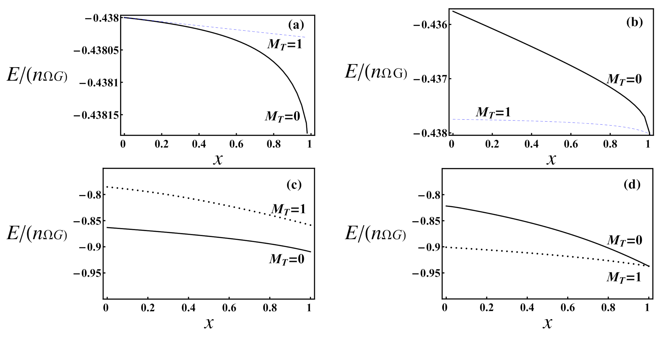
Hence, when $G_{\pi }=G_{\nu }=G_{\pi \nu }$, the lowest isospin is $\mathrm{T}=1$ when k is odd, and $\mathrm{T}=0$ when k is even. Let $G_{\pi }=G_{\nu }=G$ and $G_{\pi \nu }=x$. Figure 1 shows the lowest $M_T=0$ and $M_T=1$ level energies as functions of x for even $k=250$ shown in panel (a) and odd $k=251$ shown in panel (b) for $\mathrm{\Omega }=1000$, where the single-particle energy term is a constant and not involved in the plot. For the even k case, the $M_T=0$ level is with $\mathrm{T}=0$, while $M_T=1$ level is with $\mathrm{T}=1$ when $x=1$. The ground state in this case is always the lowest $M_T=0$ state. For the odd k case, on the contrary, there is a gap between the $M_T=0$ and $M_T=1$ levels, which gradually diminishes with the increasing of x. The $M_T=0$ and $M_T=1$ levels degenerate when $x=1$ leads to the $\mathrm{T}=1$ ground state in this case. This feature persists in realistic systems as well. For example, panels (c,d) show $M_T=0$ and $M_T=1$ levels generated from (19) for $n=12$ and $n=10$ valence particles, respectively, in the $ds$-shell with $j_1=1/2$, $j_2=3/2$ and $j_3=5/2$ orbits, for which the experimentally deduced single-particle energies above the ${}^{16}$O core with ${ϵ}_1={ϵ}_{1s_{1/2}}=-3.27$ MeV, ${ϵ}_2={ϵ}_{0p_{3/2}}=0.94$ MeV, ${ϵ}_3={ϵ}_{0d_{5/2}}=-4.14$ MeV [50], together with the nn- and pp-pairing strengths being set as $G_{\pi }=G_{\nu }=1$ MeV, are used. Due to the mean-field contribution, the energy gap between $M_T=0$ and $M_T=1$ levels is less changed with the variation of x for k even, in comparison to the single orbit case, even when $x=0$, while the two levels still degenerate when $x=1$ for odd k case leading to the $\mathrm{T}=1$ ground state.

When pj-orbits are involved in the charge-independent case with $G_{\pi }=G_{\nu }=G_{\pi \nu }$, since $\rho$ of the pairing operator $A_{\rho }^{+}$ can be taken as three different values, for a given number of pairs $k=n/2$, the possible irrep constructed by the k pairing operators $\left\{A_{\rho }^{+}\right\}$ denoted by a Young diagram ${\left[\lambda \right]}_k$ of the permutation group S${}_k$ with exactly k boxes can have three rows at most. Due to the Schur–Weyl duality relation between the permutation group S${}_k$ and the unitary group U(N), the Young diagram ${\left[\lambda \right]}_k$ of S${}_k$ can be regarded as the same irrep of U(N). Since ${\left[\lambda \right]}_k$ contains three rows at most, in this case it can be considered to be equivalent to the same irrep of U(3). Therefore, the possible isospin quantum number T for a given irrep ${\left[\lambda \right]}_k$ of S${}_k$ can be obtained by the reduction U(3) $\downarrow {\mathrm{O}}_{\mathrm{T}}\left(3\right)$ for ${\left[\lambda \right]}_k\downarrow \mathrm{T}$, of which the branching rule gives the possible values of T for given number of pairs $k=n/2$ of the system [15].

5. Model Applications to Even–Even and Odd–Odd ds-Shell Nuclei

As an application of this diagonalization scheme, some low-lying $\mathrm{J}=0^{+}$ level energies of even–even and odd–odd A = 18–28 nuclei up to the half-filling in the $ds$-shell outside the ${}^{16}$O core are fitted by the Hamiltonian (19) in the charge-independent approximation with $G_{\pi }=G_{\nu }=G_{\pi \nu }=G$, of which some results have been reported in our recent paper [46]. In order to fit binding energies of these nuclei, in addition to the mean-field plus isovector pairing, the Coulomb energy and the symmetry energy with the isospin-dependent part of the Wigner energy contribution to the binding are considered with the expression of the model Hamiltonian, the same as that used in [46,50]:

$$\widehat{H}=-\mathrm{BE}{(}^{16}\mathrm{O})+\overline{ϵ}\left(n\right)\widehat{n}+{\widehat{H}}_0+E_{\mathrm{c}}\left(\mathrm{A},\mathrm{Z}\right)-E_{\mathrm{c}}\left(16,8\right)+{\alpha }_{\mathrm{sym}}\left(\mathrm{A}\right)\mathbf{T}·\mathbf{T},$$

(26)

where ${\widehat{H}}_0$ is given by (19) with ${ϵ}_{\pi ,i}={ϵ}_{\nu ,i}={ϵ}_i$, which is the mean-field plus isovector pairing Hamiltonian (19) in the charge-independent form, $\mathrm{BE}{(}^{16}\mathrm{O})=127.619$ MeV is the binding energy of the ${}^{16}$O core taken as the experimental value, $\overline{ϵ}\left(n\right)$ is the average binding energy per valence nucleon in the $ds$-shell with $j_1=1/2$, $j_2=3/2$ and $j_3=5/2$ orbits, of which the number of valence nucleons dependent form is determined from a best fit to binding energies of all $ds$-shell nuclei considered.

$$E_{\mathrm{c}}\left(\mathrm{A},\mathrm{Z}\right)=0.699\frac{\mathrm{Z}(\mathrm{Z}-1)}{{\mathrm{A}}^{1/3}}\left(1-\frac{0.76}{{\left(\mathrm{Z}(\mathrm{Z}-1)\right)}^{1/3}}\right)\left(\mathrm{MeV}\right)$$

(27)

is the Coulomb energy [51] and

$${\alpha }_{\mathrm{sym}}\left(\mathrm{A}\right)=\frac{1}{\mathrm{A}}\left(134.4-\frac{203.6}{{\mathrm{A}}^{1/3}}\right)\left(\mathrm{MeV}\right)+\delta \alpha \left(\mathrm{A}\right)$$

(28)

is the parameter of the symmetry energy and the isospin-dependent part of the Wigner energy contribution, of which the first term is taken to be the empirical global symmetry energy paramter provided in [51], while $\delta \alpha \left(\mathrm{A}\right)$ is adjusted according to the experimental binding energy of the nucleus with a given mass number A needed to account for local deviation from the first term when the Hamiltonian (26) is used; the experimentally deduced single-particle energies above the ${}^{16}$O core with ${ϵ}_1={ϵ}_{1s_{1/2}}=-3.27$ MeV, ${ϵ}_2={ϵ}_{0p_{3/2}}=0.94$ MeV, ${ϵ}_3={ϵ}_{0d_{5/2}}=-4.14$ MeV [50] are used for the mean-field, and in order to achieve a better fit for low-lying $\mathrm{J}=0^{+}$ level energies, the overall isovector pairing strength is taken as $G=1$ MeV for all the nuclei considered. The best fit yields

$$\overline{ϵ}\left(n\right)=-2.3325-0.2000n-0.0125n^2\left(\mathrm{MeV}\right),$$

(29)

of which the first constant is very close to the value of the average binding energy per valence nucleon with ${ϵ}_{\mathrm{avg}}=-2.301$ MeV used in [50]; the contribution from the second term to the binding related to the two-body interaction becomes smaller because relatively larger pairing strength is used in the present calculation, while the third term is related to the three-body interaction as further correction. The parameter $\delta \alpha \left(\mathrm{A}\right)$ obtained from the fitting procedure is provided in

Table 1. The value of $\delta \alpha \left(\mathrm{A}\right)$ (in MeV) of (28) obtained by fitting to the binding energies and some low-lying $\mathrm{J}=0^{+}$ level energies of even–even and odd–odd A = 18–28 nuclei in this model.

A	18	20	22	24	26	28
$\delta$(A)	−0.025	−0.700	−0.940	−0.500	1.900	−0.005

.

Since the binding energies and a few low-lying J${}^{\pi }$ = 0${}^{+}$ level energies of even–even and odd–odd A = 18–28 nuclei were fit together, deviations remain between the fitted values and experimental binding energies shown in

Table 2. Binding energies BE${}_{\mathrm{th}}$ (in MeV) of 22 even–even and odd–odd nuclei with valence nucleons confined to the $ds$-shell up to the half-filled level fit by the mean-field plus charge-independent isovector pairing Hamiltonian (26) with its parameters shown in the text, where n is the number of valence nucleons in the corresponding nucleus, $E_n^{\left(1\right)}$ (in MeV) is the lowest eigen-energy of (19) and the experimental binding energy BE${}_{\exp }$ (in MeV) of these nuclei is taken from [53].

Nucleus	n	Isospin	${\mathit{E}}_{\mathit{n}}^{\left(1\right)}$	BE${}_{\mathbf{th}}$	BE${}_{\mathbf{exp}}$
${}_8^{18}$O${}_{10}$	2	$\mathrm{T}=1$	−13.788	140.000	139.808
${}_9^{18}$F${}_9$	2	$\mathrm{T}=1$	−13.788	137.313	137.369
${}_{10}^{18}$Ne${}_8$	2	$\mathrm{T}=1$	−13.788	132.035	132.143
${}_8^{20}$O${}_{12}$	4	$\mathrm{T}=2$	−25.378	151.201	151.371
${}_9^{20}$F${}_{11}$	4	$\mathrm{T}=1$	−21.870	154.405	154.403
${}_{10}^{20}$Ne${}_{10}$	4	$\mathrm{T}=0$	−28.653	160.405	160.645
${}_{11}^{20}$Na${}_9$	4	$\mathrm{T}=1$	−21.870	145.965	145.970
${}_{12}^{20}$Mg${}_8$	4	$\mathrm{T}=2$	−25.378	133.839	134.561
${}_8^{22}$O${}_{14}$	6	$\mathrm{T}=3$	−34.674	161.446	162.037
${}_{10}^{22}$Ne${}_{12}$	6	$\mathrm{T}=1$	−40.242	178.228	177.770
${}_{11}^{22}$Na${}_{11}$	6	$\mathrm{T}=1$	−40.242	174.144	174.145
${}_{12}^{22}$Mg${}_{10}$	6	$\mathrm{T}=1$	−40.242	168.858	168.581
${}_{14}^{22}$Si${}_8$	6	$\mathrm{T}=3$	−34.674	133.328	133.276
${}_{10}^{24}$Ne${}_{14}$	8	$\mathrm{T}=2$	−49.538	191.600	191.840
${}_{11}^{24}$Na${}_{13}$	8	$\mathrm{T}=1$	−46.770	193.522	193.522
${}_{12}^{24}$Mg${}_{12}$	8	$\mathrm{T}=0$	−52.938	198.852	198.257
${}_{13}^{24}$Al${}_{11}$	8	$\mathrm{T}=1$	−46.770	183.113	183.590
${}_{14}^{24}$Si${}_{10}$	8	$\mathrm{T}=2$	−49.538	171.522	172.013
${}_{12}^{26}$Mg${}_{14}$	10	$\mathrm{T}=1$	−62.231	216.775	216.681
${}_{13}^{26}$Al${}_{13}$	10	$\mathrm{T}=1$	−62.231	211.66	211.894
${}_{14}^{26}$Si${}_{12}$	10	$\mathrm{T}=1$	−62.231	206.088	206.042
${}_{14}^{28}$Si${}_{14}$	12	$\mathrm{T}=0$	−72.685	247.665	247.737

with a root mean square deviation ${\sigma }_{\mathrm{BE}}=0.32$ MeV, except ${}^{22}$F and ${}^{22}$Al, for which J${}^{\pi }$ = 0${}^{+}$ level energies are not available experimentally.

Table 3. A few lowest $\mathrm{J}=0^{+}$ level energies (in MeV) of the 22 even–even and odd–odd $ds$-shell nuclei fit by (26) (Th), where ${\mathrm{T}}_{\xi }$ denotes the $\xi$-th excited levels with isospin $\mathrm{T}$, the label g denotes the ground state, the experimental data (Exp) are taken from [53], ‘—’ denotes the corresponding level is not observed experimentally, and the shell model results (SM) are obtained by using the KSHELL code [34] with the USD (W) interaction [52] and the parameters of (26) are the same as those used in fitting the binding energies.

${}^{18}$O	Exp	Th	SM	${}^{18}$F	Exp	Th	SM	${}^{18}$Ne	Exp	Th	SM
0${}^{+}$ (${\mathrm{T}}_{\xi }$ = 1${}_g$)	0	0	0	0${}^{+}$ (${\mathrm{T}}_{\xi }$ = 1${}_1$)	1.04	1.10	1.19	0${}^{+}$ (${\mathrm{T}}_{\xi }$ = 1${}_g$)	0	0	0
0${}^{+}$ (${\mathrm{T}}_{\xi }$ = 1${}_2$)	3.63	5.71	4.32	0${}^{+}$ (${\mathrm{T}}_{\xi }$ = 1${}_2$)	4.75	6.75	5.51	0${}^{+}$ (${\mathrm{T}}_{\xi }$ = 1${}_2$)	3.58	5.71	4.32
${}^{\mathbf{20}}$O	Exp	Th	SM	${}^{\mathbf{20}}$F	Exp	Th	SM	${}^{\mathbf{20}}$Ne	Exp	Th	SM
0${}^{+}$ (${\mathrm{T}}_{\xi }$ = 2${}_g$)	0	0	0	0${}^{+}$ (${\mathrm{T}}_{\xi }$ = 1${}_1$)	3.53	1.23	3.49	$0^{+}$ (${\mathrm{T}}_{\xi }$ = 0${}_g$)	0	0	0
0${}^{+}$ (${\mathrm{T}}_{\xi }$ = 2${}_2$)	4.46	5.07	5.04	0${}^{+}$ (${\mathrm{T}}_{\xi }$ = 2${}_1$)	6.52	6.80	6.52	0${}^{+}$ (${\mathrm{T}}_{\xi }$ = 0${}_2$)	6.73	5.90	6.76
								0${}^{+}$ (${\mathrm{T}}_{\xi }$ = 1${}_1$)	13.64	11.33	13.64
								0${}^{+}$ (${\mathrm{T}}_{\xi }$ = 2${}_1$)	16.73	16.90	16.66
${}^{\mathbf{20}}$Na	Exp	Th	SM	${}^{\mathbf{20}}$Mg	Exp	Th	SM
0${}^{+}$ (${\mathrm{T}}_{\xi }$ = 1${}_1$)	3.09	1.48	3.49	0${}^{+}$ (${\mathrm{T}}_{\xi }$ = 2${}_g$)	0	0	0
0${}^{+}$ (${\mathrm{T}}_{\xi }$ = 2${}_1$)	6.53	7.05	6.52	0${}^{+}$ (${\mathrm{T}}_{\xi }$ = 2${}_1$)	—	5.07	5.04
${}^{\mathbf{22}}$O	Exp	Th	SM	${}^{\mathbf{22}}$Ne	Exp	Th	SM	${}^{\mathbf{22}}$Na	Exp	Th	SM
0${}^{+}$ (${\mathrm{T}}_{\xi }$ = 3${}_g$)	0	0	0	0${}^{+}$ (${\mathrm{T}}_{\xi }$ = 1${}_1$)	0	0	0	0${}^{+}$ (${\mathrm{T}}_{\xi }$ = 1${}_1$)	0.66	0.36	0.66
0${}^{+}$ (${\mathrm{T}}_{\xi }$ = 3${}_2$)	4.91	4.35	4.62	0${}^{+}$ (${\mathrm{T}}_{\xi }$ = 1${}_2$)	6.24	5.03	6.34	0${}^{+}$ (${\mathrm{T}}_{\xi }$ = 1${}_2$)	—	5.40	7.01
${}^{\mathbf{22}}$Mg	Exp	Th	SM	${}^{\mathbf{22}}$Si	Exp	Th	SM
0${}^{+}$ (${\mathrm{T}}_{\xi }$ = 1${}_g$)	0	0	0	0${}^{+}$ (${\mathrm{T}}_{\xi }$ = 3${}_g$)	0	0	0
0${}^{+}$ (${\mathrm{T}}_{\xi }$ = 1${}_2$)	5.95	5.03	6.34
${}^{\mathbf{24}}$Ne	Exp	Th	SM	${}^{\mathbf{24}}$Na	Exp	Th	SM	${}^{\mathbf{24}}$Mg	Exp	Th	SM
0${}^{+}$ (${\mathrm{T}}_{\xi }$ = 2${}_g$)	0	0	0	0${}^{+}$ (${\mathrm{T}}_{\xi }$ = 1${}_1$)	3.68	0.37	3.33	0${}^{+}$ (${\mathrm{T}}_{\xi }$ = 0${}_g$)	0	0	0
0${}^{+}$ (${\mathrm{T}}_{\xi }$ = 2${}_2$)	4.77	4.30	4.66	0${}^{+}$ (${\mathrm{T}}_{\xi }$ = 2${}_1$)	5.97	6.23	5.88	0${}^{+}$ (${\mathrm{T}}_{\xi }$ = 0${}_2$)	6.43	5.15	7.56
								0${}^{+}$ (${\mathrm{T}}_{\xi }$ = 1${}_1$)	13.04	10.48	12.87
								0${}^{+}$ (${\mathrm{T}}_{\xi }$ = 2${}_1$)	15.44	16.35	15.43
${}^{\mathbf{24}}$Al	Exp	Th	SM	${}^{\mathbf{24}}$Si	Exp	Th	SM	${}^{\mathbf{26}}$Mg	Exp	Th	SM
0${}^{+}$ (${\mathrm{T}}_{\xi }$ = 1${}_1$)	—	0.48	3.33	0${}^{+}$ (${\mathrm{T}}_{\xi }$ = 2${}_g$)	0	0	0	0${}^{+}$ (${\mathrm{T}}_{\xi }$ = 1${}_g$)	0	0	0
0${}^{+}$ (${\mathrm{T}}_{\xi }$ = 2${}_1$)	5.96	6.35	5.88					0${}^{+}$ (${\mathrm{T}}_{\xi }$ = 1${}_2$)	3.59	4.24	3.68
								0${}^{+}$ (${\mathrm{T}}_{\xi }$ = 1${}_3$)	4.97	5.13	5.20
${}^{\mathbf{26}}$Al	Exp	Th	SM	${}^{\mathbf{26}}$Si	Exp	Th	SM	${}^{\mathbf{28}}$Si	Exp	Th	SM
0${}^{+}$ (${\mathrm{T}}_{\xi }$ = 1${}_1$)	0.23	0.23	0.08	0${}^{+}$ (${\mathrm{T}}_{\xi }$ = 1${}_g$)	0	0	0	0${}^{+}$ (${\mathrm{T}}_{\xi }$ = 0${}_g$)	0	0	0
0${}^{+}$ (${\mathrm{T}}_{\xi }$ = 1${}_2$)	3.75	4.47	3.76	0${}^{+}$ (${\mathrm{T}}_{\xi }$ = 1${}_2$)	3.36	4.24	3.68	0${}^{+}$ (${\mathrm{T}}_{\xi }$ = 0${}_2$)	4.98	4.25	5.01
0${}^{+}$ (${\mathrm{T}}_{\xi }$ = 1${}_3$)	5.20	5.36	5.29	0${}^{+}$ (${\mathrm{T}}_{\xi }$ = 1${}_3$)	4.83	5.13	5.20	0${}^{+}$ (${\mathrm{T}}_{\xi }$ = 1${}_1$)	10.27	10.27	10.29

shows the lowest experimentally known $\mathrm{J}=0^{+}$ level energies (in MeV) of these even–even and odd–odd $ds$-shell nuclei fit by (26) with the same model parameters as used in fitting the binding energies, in which the corresponding shell model results (SM) obtained by using the KSHELL code [34] with the USD (W) interaction [52] are also provided for comparison. The root mean square deviation of the fit values to these excited $\mathrm{J}=0^{+}$ level energies is ${\sigma }_{\mathrm{level}}=1.20$ MeV, while the average deviation of the excited level energies $\varphi ={\sum }_i|E_{\mathrm{Th}}^i-E_{\mathrm{Exp}}^i|/{\sum }_i{E}_{\mathrm{Exp}}^i$ appears to be $\varphi =17.4\%$, where the sum runs over all the excited level energies of these nuclei. In addition, when the ground state of the nucleus is not a J${}^{\pi }$ = 0${}^{+}$ state, which cannot be determined from present calculation for J = 0${}^{+}$ states only, the eigen-energy of (26) is given by

$$E(\xi ,\mathrm{T},\mathrm{J}=0)=-\mathrm{BE}(\mathrm{Z},\mathrm{N})+E_{\mathrm{ex}}(\xi ,\mathrm{T},\mathrm{J}=0),$$

(30)

where $E_{\mathrm{ex}}(\xi ,\mathrm{T},\mathrm{J}=0)>0$ is the excitation energy of the $\xi$-th excited state with isospin T and J = 0. The theoretical value of $\mathrm{BE}(\mathrm{Z},\mathrm{N})$ is adjusted to reproduce a reasonable value of the excitation energy $E_{\mathrm{ex}}(\xi ,\mathrm{T},\mathrm{J}=0)$. Due to the Coulomb energy contribution and the freedom in adjusting the binding energy with a reasonable value of the excitation energy in this case, there is about a few hundreds of keV energy difference in these excitation energies of mirror nuclei with J ≠ 0 ground state, as shown in Table 3.

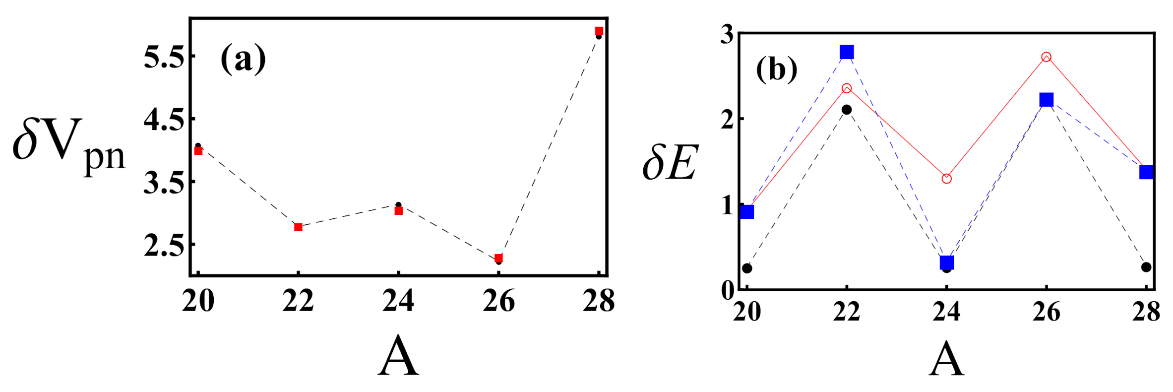
Panel (a) of Figure 2 shows the double binding-energy difference defined as [54]

$$\delta {\mathrm{V}}_{\mathrm{pn}}=\frac{1}{4}\left(\mathrm{BE}(\mathrm{Z},\mathrm{N})-\mathrm{BE}(\mathrm{Z}-2,\mathrm{N})-\mathrm{BE}(\mathrm{Z},\mathrm{N}-2)+\mathrm{BE}(\mathrm{Z}-2,\mathrm{N}-2)\right)$$

(31)

calculated by using the binding energies of both the related even–even and odd–odd nuclei Included in the fitting procedure, which shows that the experimental data are well-fit by the model Hamiltonian (26). Moreover, it is clearly shown in panel (a) of Figure 2 that $\delta {\mathrm{V}}_{\mathrm{pn}}$ becomes comparatively smaller for odd–odd N = Z nuclei with A = 22 and 26 in this case. Since the one- and two-body interaction dominating average binding energy term and the Coulomb energy term of (26) only contribute a Z and N independent constat to $\delta {\mathrm{V}}_{\mathrm{pn}}$, the symmetry energy and the isospin-dependent part of the Wigner energy term seem to be the main source that alters the usual pairing gap staggering pattern, which is consistent to the claim made in [6] that the double-binding energy difference (31) actually reveals the evidence for the Wigner energy contribution to the binding, where the usual staggering pattern of the pairing gaps disappears [50]. Alternatively, instead of $\mathrm{BE}(\mathrm{Z},\mathrm{N})$, we calculate the double pairing energy difference defined as

$$\delta E=\frac{1}{4}\left(E^{\left(1\right)}\left(\mathrm{Z},\mathrm{N}\right)-E^{\left(1\right)}\left(\mathrm{Z}-2,\mathrm{N}\right)-E^{\left(1\right)}\left(\mathrm{Z},\mathrm{N}-2\right)+E^{\left(1\right)}\left(\mathrm{Z}-2,\mathrm{N}-2\right)\right),$$

(32)

where

$$E^{\left(1\right)}\left(\mathrm{Z},\mathrm{N}\right)=\langle \xi =1,n,\mathrm{T}{M}_T|{\widehat{H}}_{\mathrm{P}}|\xi =1,n,\mathrm{T}{M}_T\rangle ,$$

(33)

in which $|\xi =1,n,\mathrm{T}{M}_T\rangle$ is the lowest eigenstate of the model, with either ${\widehat{H}}_{\mathrm{P}}=G{\sum }_{\rho }{A}_{\rho }^{+}{A}_{\rho }$ or ${\widehat{H}}_{\mathrm{P}}=G{A}_0^{+}{A}_0$, of which the first one is the total pairing energy contribution, while the second one is the np-pairing energy contribution to the binding. By substituting $\mathrm{BE}(\mathrm{Z},\mathrm{N})$ used in (31) with

$$\widetilde{\mathrm{BE}}(\mathrm{Z},\mathrm{N})=\mathrm{BE}(\mathrm{Z},\mathrm{N})+\frac{1}{\mathrm{A}}\left(134.4-\frac{203.6}{{\mathrm{A}}^{1/3}}\right)\mathrm{T}(\mathrm{T}+1)\left(\mathrm{MeV}\right),$$

(34)

which removes the symmetry energy and the isospin-dependent part of the Wigner energy contribution to the binding energy, the resultant $\widetilde{\delta {\mathrm{V}}_{\mathrm{pn}}}$ obtained from (31) should be close to the double-pairing energy difference (32). And indeed, as shown in panel (b) of Figure 2, the value of $\widetilde{\delta {\mathrm{V}}_{\mathrm{pn}}}$ is very close to one of the $\delta E$ values calculated with the total pairing energy contribution and that with the np-pairing energy contribution. Most noticeably, the staggering pattern appears, and the actual np-pairing energy in the odd–odd N = Z nuclei turns to be comparatively strong.

Table 4. The np-, nn- and pp-pairing energy contribution (in MeV) to the binding energy of the 22 even–even and odd–odd $ds$-shell nuclei, the average number of the np-pairs $k_{\mathrm{np}}$ and its fluctuation $\Delta k_{\mathrm{np}}$ and the np-pair occupation number ${\zeta }_{\mathrm{np}}$ in the J = 0${}^{+}$ ground state or the lowest J = 0${}^{+}$ excited state.

Nucleus	n	Isospin	${\mathit{E}}_{\mathbf{np}}^{\left(1\right)}$	${\mathit{E}}_{\mathbf{nn}}^{\left(1\right)}$	${\mathit{E}}_{\mathbf{pp}}^{\left(1\right)}$	${\mathit{\eta }}_{\mathbf{np}}$	${\mathit{k}}_{\mathbf{np}}$	$\mathbf{\Delta }{\mathit{k}}_{\mathbf{np}}$	${\mathit{k}}_{\mathbf{nn}}$	${\mathit{k}}_{\mathbf{pp}}$	${\mathit{\zeta }}_{\mathbf{np}}$
${}_8^{18}$O${}_{10}$	2	$\mathrm{T}=1$	0	5.036	0	0%	0	0	1	0	0%
${}_9^{18}$F${}_9$	2	$\mathrm{T}=1$	5.036	0	0	100%	1	0	0	0	100%
${}_{10}^{18}$Ne${}_8$	2	$\mathrm{T}=1$	0	0	5.036	0%	0	0	0	1	0%
${}_8^{20}$O${}_{12}$	4	$\mathrm{T}=2$	0	7.945	0	0%	0	0	2	0	0%
${}_9^{20}$F${}_{11}$	4	$\mathrm{T}=1$	2.568	2.568	0	50%	1	0	1	0	50%
${}_{10}^{20}$Ne${}_{10}$	4	$\mathrm{T}=0$	3.707	3.707	3.707	33.33%	0.497	0.865	0.7515	0.7515	24.85%
${}_{11}^{20}$Na${}_9$	4	$\mathrm{T}=1$	2.568	0	2.568	50%	1	0	0	1	50%
${}_{12}^{20}$Mg${}_8$	4	$\mathrm{T}=2$	0	0	7.945	0%	0	0	0	2	0%
${}_8^{22}$O${}_{14}$	6	$\mathrm{T}=3$	0	8.666	0	0%	0	0	3	0	0%
${}_{10}^{22}$Ne${}_{12}$	6	$\mathrm{T}=1$	2.226	7.356	4.444	15.87%	0.205	0.606	1.8975	0.8975	6.83%
${}_{11}^{22}$Na${}_{11}$	6	$\mathrm{T}=1$	9.573	2.226	2.226	68.25%	1.756	0.940	0.622	0.622	58.53%
${}_{12}^{22}$Mg${}_{10}$	6	$\mathrm{T}=1$	2.226	4.444	7.356	15.87%	0.205	0.606	0.8975	1.8975	6.83%
${}_{14}^{22}$Si${}_8$	6	$\mathrm{T}=3$	0	0	8.666	0%	0	0	0	3	0%
${}_{10}^{24}$Ne${}_{14}$	8	$\mathrm{T}=2$	1.600	8.393	4.756	10.85%	0.083	0.159	2.9585	0.9585	2.08%
${}_{11}^{24}$Na${}_{13}$	8	$\mathrm{T}=1$	5.061	4.167	2.681	42.49%	1.404	0.645	1.798	0.798	35.10%
${}_{12}^{24}$Mg${}_{12}$	8	$\mathrm{T}=0$	6.000	6.000	6.000	33.33%	0.711	1.342	1.6445	1.6445	17.78%
${}_{13}^{24}$Al${}_{11}$	8	$\mathrm{T}=1$	5.061	2.681	4.167	42.49%	1.404	0.645	0.798	1.798	35.10%
${}_{14}^{24}$Si${}_{10}$	8	$\mathrm{T}=2$	1.600	4.756	8.393	10.85%	0.083	0.159	0.9585	2.9585	2.08%
${}_{12}^{26}$Mg${}_{14}$	10	$\mathrm{T}=1$	3.615	7.917	7.186	19.31%	0.234	0.449	2.883	1.883	4.68%
${}_{13}^{26}$Al${}_{13}$	10	$\mathrm{T}=1$	11.489	3.615	3.615	61.38%	1.792	1.179	1.604	1.604	35.84%
${}_{14}^{26}$Si${}_{12}$	10	$\mathrm{T}=1$	3.615	7.186	7.917	19.31%	0.234	0.449	1.883	2.883	4.68%
${}_{14}^{28}$Si${}_{14}$	12	$\mathrm{T}=0$	6.847	6.847	6.847	33.33%	0.585	1.066	2.7075	2.7075	9.75%

shows actual nn-, pp- and np-pairing contribution at the ground state or the lowest eigenstate of (26) for these nuclei defined by -4.6cm0cm

$$\begin{array}{cc}\hfill & E_{\mathrm{np}}^{\left(1\right)}=G\langle \xi =1,n,\mathrm{T}{M}_T|A_0^{+}{A}_0|\xi =1,n,\mathrm{T}{M}_T\rangle ,E_{\mathrm{nn}}^{\left(1\right)}=G\langle \xi =1,n,\mathrm{T}{M}_T|A_{-1}^{+}{A}_{-1}|\xi =1,n,\mathrm{T}{M}_T\rangle ,\\ & E_{\mathrm{pp}}^{\left(1\right)}=G\langle \xi =1,n,\mathrm{T}{M}_T|A_1^{+}{A}_1|\xi =1,n,\mathrm{T}{M}_T\rangle ,\end{array}$$

(35)

and the percentage of the np-pairing energy contribution to the binding ${\eta }_{\mathrm{np}}=E_{\mathrm{np}}^{\left(1\right)}/(E_{\mathrm{np}}^{\left(1\right)}+E_{\mathrm{nn}}^{\left(1\right)}+E_{\mathrm{pp}}^{\left(1\right)})$. It can be observed that $E_{\mathrm{nn}}^{\left(1\right)}$ in the N = Z + 2 nuclei is the same as $E_{\mathrm{pp}}^{\left(1\right)}$ in the Z = N + 2 mirror nuclei, while $E_{\mathrm{nn}}^{\left(1\right)}=E_{\mathrm{pp}}^{\left(1\right)}$ in the N = Z nuclei due to the charge-independent isovector pairing is adopted. However, $E_{\mathrm{np}}^{\left(1\right)}=E_{\mathrm{nn}}^{\left(1\right)}=E_{\mathrm{pp}}^{\left(1\right)}$ in even–even N = Z nuclei, while $E_{\mathrm{np}}^{\left(1\right)}>E_{\mathrm{nn}}^{\left(1\right)}=E_{\mathrm{pp}}^{\left(1\right)}$ in odd–odd N = Z nuclei, which shows that the np-pairing energy contribution to the binding is the largest in odd–odd N = Z nuclei.

Since the total number of valence nucleons n and the total isospin projection $M_T$ are good quantum numbers of the system, the number of valence protons and that of valence neutrons are certainly fixed in each nucleus with $n_{\pi }=(n+2M_T)/2$ and $n_{\nu }=(n-2M_T)/2$, respectively. As shown in Section 3, the number of np-pairs in the i-th orbit can be defined as $q_i={\mathrm{\Omega }}_i-2{\mathrm{\Lambda }}_i$ within the seniority-zero configuration, where the neutron (proton) quasi-spin ${\mathrm{\Lambda }}_i$ is a good quantum number in the O(5) tensor product basis adapted to the ${\mathrm{SU}}_{\mathrm{\Lambda }}\left(2\right)\otimes {\mathrm{SU}}_I\left(2\right)\supset {\mathrm{U}}_{\mathrm{\Lambda }}\left(1\right)\otimes {\mathrm{U}}_I\left(1\right)$ chain. Therefore, the average number of the np-pairs in the lowest J = $0^{+}$ state of the model can be defined as

$$k_{\mathrm{np}}=\langle \xi =1,n,\mathrm{T}{M}_T|\widehat{q}|\xi =1,n,\mathrm{T}{M}_T\rangle ,$$

(36)

with $\widehat{q}={\sum }_{i=1}^p({\mathrm{\Omega }}_i-2{\widehat{\mathrm{\Lambda }}}_i)$. Thus, the average number of nn-pairs and that of pp-pairs are given by

$$k_{\mathrm{nn}}=(n_{\nu }-k_{\mathrm{np}})/2,k_{\mathrm{pp}}=(n_{\pi }-k_{\mathrm{np}})/2.$$

(37)

$k_{\mathrm{np}}$, $k_{\mathrm{nn}}$, and $k_{\mathrm{pp}}$ values for each nucleus at the lowest J = 0${}^{+}$ state are shown in Table 4. Since the number of np-pairs is not a conserved quantity, its fluctuation in the lowest J = 0${}^{+}$ state of these nuclei defined as

$$\Delta k_{\mathrm{np}}={\left(\langle \xi =1,n,\mathrm{T}{M}_T\left|{\left(\widehat{q}-k_{\mathrm{np}}\right)}^2\right|\xi =1,n,\mathrm{T}{M}_T\rangle \right)}^{1/2}$$

(38)

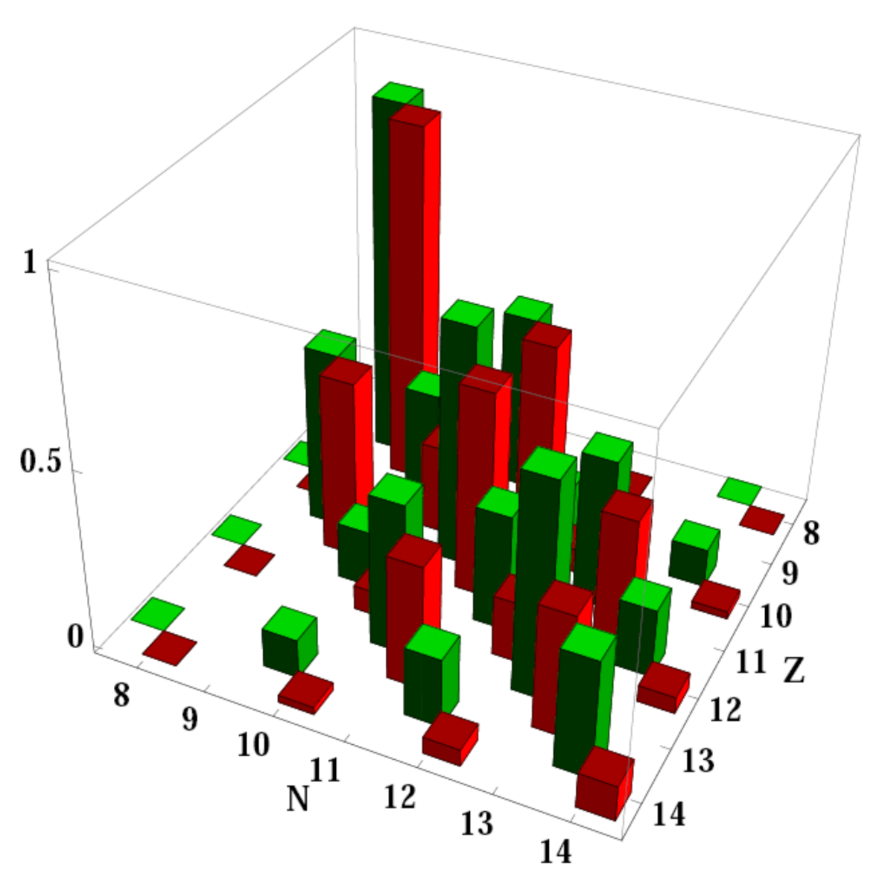
is also provided. It can be observed from Table 4 that the $k_{\mathrm{np}}$ value is a definite integer for nuclei with less than or equal to one valence neutron or proton, for which the $k_{\mathrm{np}}$ value is also easily countable, while (38) must be used for evaluating $k_{\mathrm{np}}$ for nuclei with more valence neutrons and protons. It is obvious that the $k_{\mathrm{np}}$ value is indeed relatively large in the odd–odd N = Z nuclei, which is consistent with the larger np-pairing energy contribution to the binding shown in Table 4, while the average number of the np-pairs $k_{\mathrm{np}}$ in the even–even nuclei is considerably small with very large fluctuation. For example, $k_{\mathrm{np}}=0.711$ with $\Delta k_{\mathrm{np}}=1.342$ in ${}^{24}$Mg, while $k_{\mathrm{np}}=0.585$ with $\Delta k_{\mathrm{np}}=1.066$ in ${}^{28}$Si. The $\Delta k_{\mathrm{np}}$ value in these even–even N = Z nuclei is almost two times of the corresponding average value. Though the np-pair occupation number defined as ${\zeta }_{\mathrm{np}}=k_{\mathrm{np}}/k$ in the even–even N = Z nuclei is small, the np-pairing energy contribution is still comparable to the nn- or pp-pairing energy contribution. Using the data shown in Table 4, one can check that the np-pairing energy per np-pair $E_{\mathrm{np}}^{\left(1\right)}/k_{\mathrm{np}}$ is 2.31 and 4.63 times of $E_{\mathrm{nn}}^{\left(1\right)}/k_{\mathrm{nn}}=E_{\mathrm{pp}}^{\left(1\right)}/k_{\mathrm{pp}}$ in ${}^{24}$Mg and ${}^{28}$Si, respectively. As shown in Figure 3, the distribution of either the percentage of the np-pairing energy ${\eta }_{\mathrm{np}}$ or the np-pair occupation number ${\zeta }_{\mathrm{np}}$ is symmetric with respect to the N = Z line owing to the charge-independent approximation with the clear even–odd staggering pattern along the lines parallel to the N = Z line on the N-Z plane, where the nuclei with fixed $M_T$ are connected by each line. In short, the np-pairing is more favored in odd–odd N = Z nuclei as described by the charge-independent isovector pairing model.

Finally, np-pair stripping reactions, such as ($\alpha$, d) or (${}^3$He, p), or the corresponding picking-up process, should be sensitive tests for np-pairing correlations in nuclei, for which the np-pair amplitude determined by the matrix elements of the np-pair operator in target and product states are of importance. Here, we only calculate the np-pair amplitude contributed from the q-th orbit defined as

$$B(j_q;{\xi }_f{T}_f;{\xi }_i{T}_i;M_T)=\frac{2}{\pi }|\langle {\xi }_f;n+2;T_f{M}_T|A_0^{†}\left(j_q\right)|{\xi }_i,n;T_i{M}_T{\rangle |}^2$$

(39)

with $M_T=0$ for N = Z nuclei, where $|{\xi }_i,n;T_i{M}_T\rangle$ and $|{\xi }_f,n+2;T_f{M}_T\rangle$ are eigenstate of the isovector pairing model for target nucleus with n valence nucleons and that of product nuclei with $n+2$ valence nucleons of total angular momentum J = 0, respectively, and the expression is consistent with that shown in (4.15) of [55]. The matrix elements of $A_0^{†}\left(j_q\right)$ in the O(5) tensor product basis used in the expansion of (20) are given by

$$\begin{array}{c}\left.〈\begin{array}{c}({\mathrm{\Omega }}_1,0)\cdots ({\mathrm{\Omega }}_q,0)\cdots ({\mathrm{\Omega }}_p,0)\hfill \\ {\mathrm{\Lambda }}_1^{\prime }\cdots {\mathrm{\Lambda }}_q^{\prime }\cdots {\mathrm{\Lambda }}_p^{\prime }\hfill \\ n_1^{\prime },m_T^{\prime }\left(1\right)\cdots n_q^{\prime },m_T^{\prime }\left(q\right)\cdots n_p^{\prime },m_T^{\prime }\left(p\right)\hfill \end{array}\right|A_0^{+}\left(j_q\right)\left|\begin{array}{c}({\mathrm{\Omega }}_1,0)\cdots ({\mathrm{\Omega }}_q,0)\cdots ({\mathrm{\Omega }}_p,0)\hfill \\ {\mathrm{\Lambda }}_1\cdots {\mathrm{\Lambda }}_q\cdots {\mathrm{\Lambda }}_p\hfill \\ n_1,m_T\left(1\right)\cdots n_q,m_T\left(q\right)\cdots n_p,m_T\left(p\right)\hfill \end{array}\right.〉=\end{array}$$

$$\begin{array}{cc}& {\prod }_{i\ne q}^p{\delta }_{{\mathrm{\Lambda }}_i^{\prime }{\mathrm{\Lambda }}_i}{\delta }_{{\mu }_i^{\prime }{\mu }_i}{\delta }_{{\nu }_i^{\prime }{\nu }_i}{\delta }_{{\mu }_q^{\prime }{\mu }_q+\frac{1}{2}}{\delta }_{{\nu }_q^{\prime }{\nu }_q+\frac{1}{2}}\left({\delta }_{{\mathrm{\Lambda }}_q^{\prime }{\mathrm{\Lambda }}_q+\frac{1}{2}}\langle {\mathrm{\Lambda }}_q{\mu }_q\frac{1}{2}\frac{1}{2}|{\mathrm{\Lambda }}_q+\frac{1}{2}{\mu }_q+\frac{1}{2}\rangle \langle {\mathrm{\Lambda }}_q{\nu }_q\frac{1}{2}\frac{1}{2}|{\mathrm{\Lambda }}_q+\frac{1}{2}{\nu }_q+\frac{1}{2}\rangle \times \right.\\ \hfill & {\left(\frac{({\mathrm{\Omega }}_q+2{\mathrm{\Lambda }}_q+3)({\mathrm{\Omega }}_q-2{\mathrm{\Lambda }}_q)(2{\mathrm{\Lambda }}_q+1)}{2(2{\mathrm{\Lambda }}_q+2)}\right)}^{\frac{1}{2}}+{\delta }_{{\mathrm{\Lambda }}_q^{\prime }{\mathrm{\Lambda }}_q-\frac{1}{2}}\langle {\mathrm{\Lambda }}_q{\mu }_q\frac{1}{2}\frac{1}{2}|{\mathrm{\Lambda }}_q+\frac{1}{2}{\mu }_q+\frac{1}{2}\rangle \langle {\mathrm{\Lambda }}_q{\nu }_q\frac{1}{2}\frac{1}{2}|{\mathrm{\Lambda }}_q-\frac{1}{2}{\nu }_q+\frac{1}{2}\rangle \times \\ & \left.{\left(\frac{({\mathrm{\Omega }}_q+2{\mathrm{\Lambda }}_q+2)({\mathrm{\Omega }}_q-2{\mathrm{\Lambda }}_q+1)(2{\mathrm{\Lambda }}_q+1)}{2\left(2{\mathrm{\Lambda }}_q\right)}\right)}^{\frac{1}{2}}\right),\end{array}$$

(40)

which is used in calculating the np-pair amplitude contributed from the q-th orbit shown in (39).

It is obvious that the selection rule for (39) is $\Delta \mathrm{T}=+1,-1$. The np-pair amplitudes in the $ds$-shell with $|\Delta \mathrm{T}|=1$ are shown in

Table 5. The np-pair amplitude contributed from each j-orbit defined in (39) for $ds$-shell N = Z nuclei.

	$\mathit{j}=1/2$	$\mathit{j}=3/2$	$\mathit{j}=5/2$
B(j; ${}^{20}$Ne,T = 0${}_g$; ${}^{18}$F,T = 1${}_1$)	0.060	0.041	1.186
B(j; ${}^{20}$Ne,T = 0${}_2$; ${}^{18}$F,T = 1${}_1$)	0.207	0.001	0.114
B(j; ${}^{20}$Ne,T = 2${}_1$; ${}^{18}$F,T = 1${}_1$)	0.113	0.081	1.476
B(j; ${}^{20}$Ne,T = 0${}_g$; ${}^{18}$F,T = 1${}_2$)	0.002	≈0	0.003
B(j; ${}^{20}$Ne,T = 0${}_2$; ${}^{18}$F,T = 1${}_2$)	0.097	0.022	0.468
B(j; ${}^{20}$Ne,T = 2${}_1$; ${}^{18}$F,T = 1${}_2$)	0.018	≈0	0.033
B(j; ${}^{22}$Na,T = 1${}_1$; ${}^{20}$Ne,T = 0${}_g$)	0.144	0.100	1.837
B(j; ${}^{22}$Na,T = 1${}_1$; ${}^{20}$Ne,T = 0${}_2$)	0.012	≈0	0.021
B(j; ${}^{22}$Na,T = 1${}_1$; ${}^{20}$Ne,T = 2${}_1$)	0.049	0.033	0.945
B(j; ${}^{24}$Mg,T = 0${}_g$; ${}^{22}$Na,T = 1${}_1$)	0.120	0.081	1.751
B(j; ${}^{24}$Mg,T = 0${}_2$; ${}^{22}$Na,T = 1${}_1$)	0.150	0.001	0.075
B(j; ${}^{24}$Mg,T = 2${}_1$; ${}^{22}$Na,T = 1${}_1$)	0.152	0.109	1.269
B(j; ${}^{26}$Al,T = 1${}_1$; ${}^{24}$Mg,T = 0${}_g$)	0.195	0.136	1.570
B(j; ${}^{26}$Al,T = 1${}_2$; ${}^{24}$Mg,T = 0${}_g$)	0.192	0.003	0.083
B(j; ${}^{26}$Al,T = 1${}_3$; ${}^{24}$Mg,T = 0${}_g$)	0.007	≈0	0.004
B(j; ${}^{26}$Al,T = 1${}_1$; ${}^{24}$Mg,T = 0${}_2$)	0.045	≈0	0.088
B(j; ${}^{26}$Al,T = 1${}_2$; ${}^{24}$Mg,T = 0${}_2$)	0.058	0.019	0.775
B(j; ${}^{26}$Al,T = 1${}_3$; ${}^{24}$Mg,T = 0${}_2$)	0.118	0.077	0.927
B(j; ${}^{26}$Al,T = 1${}_1$; ${}^{24}$Mg,T = 2${}_1$)	0.099	0.064	1.388
B(j; ${}^{26}$Al,T = 1${}_2$; ${}^{24}$Mg,T = 2${}_1$)	0.002	≈0	≈0
B(j; ${}^{26}$Al,T = 1${}_3$; ${}^{24}$Mg,T = 2${}_1$)	0.187	0.001	0.094
B(j; ${}^{28}$Si,T = 0${}_g$; ${}^{26}$Al,T = 1${}_1$)	0.181	0.117	1.726
B(j; ${}^{28}$Si,T = 0${}_2$; ${}^{26}$Al,T = 1${}_1$)	0.087	0.001	0.037
B(j; ${}^{28}$Si,T = 0${}_g$; ${}^{26}$Al,T = 1${}_2$)	0.006	≈0	0.015
B(j; ${}^{28}$Si,T = 0${}_2$; ${}^{26}$Al,T = 1${}_2$)	0.138	0.064	0.908
B(j; ${}^{28}$Si,T = 0${}_g$; ${}^{26}$Al,T = 1${}_3$)	0.097	≈0	0.192
B(j; ${}^{28}$Si,T = 0${}_2$; ${}^{26}$Al,T = 1${}_3$)	0.065	0.020	0.976

. As estimated in [55], in which the single-particle energies of the mean-field were taken to be degenerate, and the isospin was not considered explicitly; the amplitude for the reactions among the J = 0${}^{+}$ ground states or the lowest J = 0${}^{+}$ excited states only depends on j with $\overline{B}\left(j\right)=(j^2+2j+3/4)/\left(2\pi \right)$, from which one achieves $\overline{B}(1/2)=0.318$, $\overline{B}(3/2)=0.955$ and $\overline{B}(5/2)=1.910$. The $\overline{B}(5/2)$ value is indeed very close to the values of (39) for the reactions among the lowest J = 0${}^{+}$ states shown in Table 5 because the $j=5/2$ orbit is the lowest in energy. Nevertheless, the amplitude for the $j=3/2$ orbit shown in Table 5 are one or two orders of magnitude smaller than $\overline{B}(3/2)$, mainly due to the fact that there is a $0.87$ MeV gap between the $j=3/2$ and the $j=5/2$ orbit. Since the $j=1/2$ orbit is the highest in energy, the corresponding amplitudes shown in Table 5 are also systematically smaller than $\overline{B}(1/2)$.

6. Summary

In this work, a diagonalization scheme for the shell model mean-field plus isovector pairing Hamiltonian in the O(5) tensor product basis is adapted to accommocate quasi-spin, which means the scheme is equivalent to a $M_T$-scheme realized in the $\mathrm{O}\left(5\right)\supset {\mathrm{SU}}_{\mathrm{\Lambda }}\left(2\right)\otimes {\mathrm{SU}}_I\left(2\right)\supset {\mathrm{U}}_{\mathrm{\Lambda }}\left(1\right)\otimes {\mathrm{U}}_I\left(1\right)$ basis. Additionally, the scheme conserves a charge-independent isovector pairing interaction while accommodating isospin symmetry breaking and provides for a number operator that counts the effective number of np-pairs that can be realized in a neutron–proton quasi-spin basis.

To illustrate the vaue of the theory, the scheme was used to determine binding energies and low-lying J = $0^{+}$ excited states of even–even and odd–odd N∼Z $ds$-shell nuclei by fitting to the charge-independent isovector pairing interaction, within which the np-, nn- and pp-pairing energy contributions to the binding in the $ds$-shell nuclei were estimated. The results show that the np-pairing contribution to the binding energies of the odd–odd N = Z nuclei is systematically larger than that in the even–even nuclei.

It is also shown that the decrease in the double binding-energy difference for the odd–odd nuclei is mainly due to the symmetry energy and Wigner energy contributions that alter the pairing staggering pattern. In particular, the average number of the np-pairs in the J = 0${}^{+}$ ground state or the lowest J = 0${}^{+}$ excited state of the even–even and odd–odd $ds$-shell nuclei were evaluated. The resuts serve to show that the average number of the np-pairs $k_{\mathrm{np}}$ in the even–even N = Z nuclei is considerably smaller with large fluctuation in comparison to that in the odd–odd N = Z nuclei, which leads to the conclusion that the isovector np-pairing is more favored in odd–odd N = Z nuclei. np-pair amplitudes of given single-particle orbits of the model useful in evaluating he neutron–proton transfer reaction rates among these N = Z nuclei are also calculated.

It should be stated that the computation of the isovector np-pair number is demonstrated for the even–even and odd–odd N∼Z ds-shell nuclei described by the isovector pairing model restricted within the O(5) seniority-zero subspace only, where the isoscalar np-pairs are not involved. In order to reveal the actual np-pair contents in these N∼Z nuclei, other O(5) seniority-nonzero configurations must be considered, for which an alternative O(8) model [56,57,58] should be more convenient. Nevertheless, as has been shown in our recent work on the O(8) model [59], not only the binding energies and the low-lying J${}^{\pi }$ = 0${}^{+}$ level energies shown in Table 2 and Table 3, but also the isovector pairing energy contributions to the binding energies provided in Table 4 are the same as those calculated from the O(8) model, where the isoscalar np-pairs are also involved. Therefore, the conclusion of the present work on the isovector pairing energy contribution to the binding energies of these ds-shell nuclei is still valid even in the presence of isoscalar np-pairs.

Further applications of this scheme to the model with more j-orbits or in other major shells are straightforward, for which detailed analysis will be a part of our future work. Extensions of the algebraic scheme outlined may also be applicable to study the spontaneous symmetry breaking process in the O(5) nonlinear $\sigma$ model [41] and Heisenberg spin interaction systems [43].

References

- Goswami, A. Treatment of neutron-proton correlations. Nucl. Phys. 1964, 60, 228–240. [Google Scholar] [CrossRef]
- Goodman, A.L. Hartree–Fock–Bogoliubov theory with applications to nuclei. Adv. Nucl. Phys. 1979, 11, 263–366. [Google Scholar]
- Bes, D.R.; Broglia, R.A.; Hansen, O.; Nathan, O. Isovector pairing vibrations. Phys. Rep. 1977, 34, 1–53. [Google Scholar] [CrossRef]
- Engel, J.; Pittel, S.; Stoitsov, M.; Vogel, P.; Dukelsky, J. Neutron-proton correlations in an exactly solvable model. Phys. Rev. C 1997, 55, 1781–1788. [Google Scholar] [CrossRef] [Green Version]
- Van Isacker, P.; Warner, D.D.; Frank, A. Deuteron Transfer in N=Z Nuclei. Phys. Rev. Lett. 2005, 94, 162502. [Google Scholar]
- Warner, D.D.; Bentley, M.A.; Van Isacker, P. The role of isospin symmetry in collective nuclear structure. Nat. Phys. 2006, 2, 311–318. [Google Scholar] [CrossRef]
- Qi, C.; Blomqvist, J.; Bäck, T.; Cederwall, B.; Johnson, A.; Liotta, R.J.; Wyss, R. Spin-aligned neutron-proton pair mode in atomic nuclei. Phys. Rev. C 2011, 84, 021301. [Google Scholar] [CrossRef] [Green Version]
- Bentley, I.; Frauendorf, S. Relation between Wigner energy and proton-neutron pairing. Phys. Rev. C 2013, 88, 014322. [Google Scholar] [CrossRef] [Green Version]
- Frauendorf, S.; Macchiavelli, A.O. Overview of neutron-proton pairing. Prog. Part. Nucl. Phys. 2014, 78, 24–90. [Google Scholar] [CrossRef] [Green Version]
- Piasetzky, E.; Sargsian, M.; Frankfurt, L.; Strikman, M.; Watson, J.W. Evidence for strong dominance of proton-neutron correlations in nuclei. Phys. Rev. Lett. 2006, 97, 162504. [Google Scholar] [CrossRef] [PubMed] [Green Version]
- Hen, O.; Sargsian, M.; Weinstein, L.B.; Piasetzky, E.; Hakobyan, H.; Higinbotham, D.W.; Braverman, M.; Brooks, W.K.; Gilad, S.; Adhikari, K.P.; et al. Momentum sharing in imbalanced Fermi systems. Science 2014, 346, 614–617. [Google Scholar] [CrossRef] [Green Version]
- Andreoiu, C.; Svensson, C.E.; Afanasjev, A.V.; Austin, R.A.E.; Carpenter, M.P.; Dashdorj, D.; Finlay, P.; Freeman, S.J.; Garrett, P.E.; Greene, J.; et al. High-spin lifetime measurements in the N=Z nucleus 72Kr. Phys. Rev. C 2007, 75, 041301. [Google Scholar]
- Hecht, K.T. Five-dimensional quasispin. Exact solutions of a pairing Hamiltonian in the J–T scheme. Phys. Rev. 1965, 139, B794–B817. [Google Scholar] [CrossRef]
- Hecht, K.T. Some simple R5 Wigner coefficients and their application. Nucl. Phys. 1965, 63, 177–213. [Google Scholar] [CrossRef]
- Pan, F.; Draayer, J.P. Algebraic solutions of mean-field plus T = 1 pairing interaction. Phys. Rev. C 2002, 66, 044314. [Google Scholar] [CrossRef]
- Dukelsky, J.; Gueorguiev, V.G.; Van Isacker, P.; Dimitrova, S.; Errea, B.; Lerma, H.S. Exact solution of the isovector neutron-proton pairing Hamiltonian. Phys. Rev. Lett. 2006, 96, 072503. [Google Scholar] [CrossRef] [Green Version]
- Langanke, K.; Dean, D.J.; Radha, P.B.; Alhassid, Y.; Koonin, S.E. Shell-model Monte Carlo studies of fp-shell nuclei. Phys. Rev. C 1995, 52, 718–725. [Google Scholar] [CrossRef] [PubMed] [Green Version]
- Langanke, K.; Vogel, P.; Zheng, D.-C. Shell model Monte Carlo studies of N = Z pf-shell nuclei with pairing-plus-quadrupole Hamiltonian. Nucl. Phys. A 1997, 626, 735–750. [Google Scholar] [CrossRef] [Green Version]
- Poves, A.; Martinez-Pinedo, G. Pairing and the structure of the pf-shell N ≈ Z nuclei. Phys. Lett. B 1998, 430, 203–208. [Google Scholar] [CrossRef] [Green Version]
- Martinez-Pinedo, G.; Langanke, K.; Vogel, P. Competition of isoscalar and isovector proton-neutron pairing in nuclei. Nucl. Phys. A 1999, 651, 379–393. [Google Scholar] [CrossRef] [Green Version]
- Stoitcheva, G.; Satuła, W.; Nazarewicz, W.; Dean, D.J.; Zalewski, M.; Zduńczuk, H. High-spin intruder states in the fp-shell nuclei and isoscalar proton-neutron correlations. Phys. Rev. C 2006, 73, 061304. [Google Scholar] [CrossRef] [Green Version]
- Kaneko, K.; Sun, Y.; Mizusaki, T.; Hasegawa, M. Shell-model study for neutron-rich sd-shell nuclei. Phys. Rev. C 2011, 83, 014320. [Google Scholar] [CrossRef] [Green Version]
- Kaneko, K.; Sun, Y.; de Angelis, G. Enhancement of high-spin collectivity in N = Z nuclei by the isoscalar neutron-proton pairing. Nucl. Phys. A 2017, 957, 144–153. [Google Scholar] [CrossRef]
- Kaneko, K.; Sun, Y.; Mizusaki, T. Isoscalar neutron-proton pairing and SU(4)-symmetry breaking in Gamow-Teller transitions. Phys. Rev. C 2018, 97, 054326. [Google Scholar] [CrossRef] [Green Version]
- Sambataro, M.; Sandulescu, N. Isovector pairing in a formalism of quartets for N = Z nuclei. Phys. Rev. C 2013, 88, 061303. [Google Scholar] [CrossRef]
- Sambataro, M.; Sandulescu, N.; Johnson, C.W. Isoscalar and isovector pairing in a formalism of quartets. Phys. Lett. B 2015, 740, 137–140. [Google Scholar] [CrossRef] [Green Version]
- Sambataro, M.; Sandulescu, N. Four-body correlations in nuclei. Phys. Rev. Lett. 2015, 115, 112501. [Google Scholar] [CrossRef] [PubMed] [Green Version]
- Fu, G.J.; Zhao, Y.M.; Arima, A. Nucleon-pair approximations for low-lying states of even-even N = Z nuclei. Phys. Rev. C 2015, 91, 054322. [Google Scholar] [CrossRef]
- Fu, G.J.; Zhao, Y.M.; Arima, A. Pair correlations in low-lying T = 0 states of odd-odd nuclei with six nucleons. Phys. Rev. C 2018, 97, 024337. [Google Scholar] [CrossRef]
- Brown, B.A. The nuclear shell model towards the drip lines. Prog. Part. Nucl. Phys. 2001, 47, 517–599. [Google Scholar] [CrossRef]
- Caurier, E.; Martínez-Pinedo, G.; Nowacki, F.; Poves, A.; Zuker, A.P. The shell model as a unified view of nuclear structure. Rev. Mod. Phys. 2005, 77, 427–488. [Google Scholar] [CrossRef] [Green Version]
- Sternberg, P.; Ng, E.G.; Yang, C.; Maris, P.; Vary, J.P.; Sosonkina, M.; Le, H.V. Accelerating configuration interaction calculations for nuclear structure. In Proceedings of the 2008 ACM/IEEE Conference on Supercomputing, Austin, TX, USA, 15–21 November 2008. [Google Scholar]
- Brown, B.A.; Rae, W.D.M. The Shell-model code NuShellX@MSU. Nucl. Data Sheets 2014, 120, 115–118. [Google Scholar] [CrossRef]
- Shimizu, N.; Mizusaki, T.; Utsuno, T.; Tsunoda, Y. Thick-restart block Lanczos method for large-scale shell-model calculations. Comput. Phys. Commun. 2019, 244, 372–384. [Google Scholar] [CrossRef] [Green Version]
- Elliott, J.P. Collective motion in the nuclear shell model. I. Classification schemes for states of mixed configurations. Proc. R. Soc. Lond. Ser. A Math. Phys. Sci. 1958, 245, 128–145. [Google Scholar]
- Elliott, J.P. Collective motion in the nuclear shell model II. The introduction of intrinsic wave-functions. Proc. R. Soc. Lond. Ser. A Math. Phys. Sci. 1958, 245, 562–581. [Google Scholar]
- Elliott, J.P.; Harvey, M. Collective motion in the nuclear shell model III. The calculation of spectra. Proc. R. Soc. Lond. Ser. A Math. Phys. Sci. 1963, 272, 557–577. [Google Scholar]
- Moshinsky, M.; Chacón, E.; Flores, J.; deLIano, M.; Mello, P.A. Group Theory and the Many-Body Problem; Gordon and Breach Scince Publishers Inc.: New York, NY, USA, 1968. [Google Scholar]
- Draayer, J.P.; Dytrych, T.; Launey, K.D.; Langr, D. Symmetry-adapted no-core shell model applications for light nuclei with QCD-inspired interactions. Prog. Part. Nucl. Phys. 2012, 67, 516–520. [Google Scholar] [CrossRef]
- Launey, K.D.; Dytrych, T.; Draayer, J.P. Symmetry-guided large-scale shell-model theory. Prog. Part. Nucl. Phys. 2016, 89, 101–136. [Google Scholar] [CrossRef] [Green Version]
- Zhang, S.-C. A unified theory based on SO(5) symmetry of superconductivity and antiferromagnetism. Science 1997, 275, 1089–1096. [Google Scholar] [CrossRef]
- Nambu, Y. Axial vector conservation in weak interactions. Phys. Rev. Lett. 1960, 4, 380–382. [Google Scholar] [CrossRef] [Green Version]
- Brauner, T. Spontaneous symmetry breaking and Nambu-Goldstone bosons in quantum many-body systems. Symmetry 2010, 2, 609–657. [Google Scholar] [CrossRef] [Green Version]
- Arraut, I. The quantum Yang-Baxter conditions: The fundamental relations behind the Nambu-Goldstone theorem. Symmetry 2019, 11, 803. [Google Scholar] [CrossRef] [Green Version]
- Pan, F.; Launey, K.D.; Draayer, J.P. Algebraic solution of the isovector pairing problem. In Proceedings of the International Conference ‘Nuclear Theory in the Supercomputing Era—2018’, Daejeon, Korea, 29 October–2 November 2018; pp. 73–82. [Google Scholar]
- Pan, F.; Qi, C.; Dai, L.; Sargsyan, G.; Launey, K.D.; Draayer, J.P. On the importance of np-pairs in the isovector pairing model. Europhys. Lett. (EPL) 2020, 132, 32001. [Google Scholar] [CrossRef]
- Moshinsky, M.; Quesne, C. Generalization to arbitrary groups of the relation between seniority and quasispin. Phys. Lett. B 1969, 29, 482–484. [Google Scholar] [CrossRef]
- Hecht, K.T. Wigner coefficients for the proton-neutron quasispin group: An application of vector coherent state techniques. Nucl. Phys. A 1989, 493, 29–60. [Google Scholar] [CrossRef] [Green Version]
- Pan, F.; Ding, X.; Launey, K.D.; Draayer, J.P. A simple procedure for construction of the orthonormal basis vectors of irreducible representations of O(5) in the OT(3)⊗ON(2) basis. Nucl. Phys. A 2018, 974, 86–105. [Google Scholar] [CrossRef]
- Miora, M.E.; Launey, K.D.; Kekejian, D.; Pan, F.; Draayer, J.P. Exact isovector pairing in a shell-model framework: Role of proton-neutron correlations in isobaric analog states. Phys. Rev. C 2019, 100, 064310. [Google Scholar] [CrossRef] [Green Version]
- Vogel, P. Pairing and symmetry energy in N≈Z nuclei. Nucl. Phys. A 2000, 662, 148–154. [Google Scholar] [CrossRef] [Green Version]
- Brown, B.A.; Wildenthal, B.H. Status of the nuclear shell model. Annu. Rev. Nucl. Part. Sci. 1988, 38, 29–66. [Google Scholar] [CrossRef]
- NuDat 2.8, National Nuclear Data Center (Brookhaven National Laboratory). Available online: http://www.nndc.bnl.gov/nudat2 (accessed on 4 May 2021).
- Zhang, J.-Y.; Casten, R.F.; Brenner, D.S. Empirical proton-neutron interaction energies. Linearity and saturation phenomena. Phys. Lett. B 1989, 227, 1–5. [Google Scholar] [CrossRef]
- Fröbrich, P. The effect of neutron-proton pairing correlations on the transfer of a neutron-proton pair. Z. Phys. 1970, 236, 153–165. [Google Scholar] [CrossRef]
- Flowers, B.H.; Szpikowski, S. Quasi-spin in LS coupling. Proc. Phys. Soc. 1964, 84, 673–680. [Google Scholar] [CrossRef]
- Pang, S.C. Exact solution of the pairing problem in the LST scheme. Nucl. Phys. A 1969, 128, 497–526. [Google Scholar] [CrossRef] [Green Version]
- Hecht, K.T. Coherent-state theory for the LST quasispin group. Nucl. Phys. A 1985, 444, 189–208. [Google Scholar] [CrossRef] [Green Version]
- Pan, F.; He, Y.; Wu, Y.; Wang, Y.; Launey, K.D.; Draayer, J.P. Neutron-proton pairing correction in the extended isovector and isoscalar pairing model. Phys. Rev. C 2020, 102, 044306. [Google Scholar] [CrossRef]
Figure 1.
The lowest (solid curve) and (dashed curve) level energies per particle of the model for (a) and (b) valence nucleons confined in a single orbit, (c) and (d) valence nucleons in the -shell as functions of , where , the constant single-particle energy term is not involved in (a,b), while MeV, MeV, MeV and MeV are used for (c,d).
Figure 2.
(a) The double-binding-energy difference (in MeV) defined in (31) for even–even and odd–odd -shell nuclei, where the red solid squares are the experimental data, and the (black) dots connected with the dashed lines are the results of the present model. (b) The double-pairing energy difference (in MeV) defined in (32), where the red open circles connected with the solid lines are calculated from (32) with the np-pairing energy contribution; the black solid dots connected with the dashed lines are calculated from (32) with the total pairing energy contribution and the blue solid squares connected with the dashed lines are values calculated from (31) with .
Figure 3.
(Color online). The percentage of the np-pairing energy (Green) and the np-pair occupation number (Red) in the lowest J = 0 state of even–even and odd–odd -shell nuclei described by the charge-independent mean-field plus isovector pairing model.